
The Impact of Different Filters on the Gravity Field Recovery Based on the GOCE Gradient Data


1
State Key Laboratory of Geodesy and Earth’s Dynamics, Innovation Academy for Precision Measurement Science and Technology, Chinese Academy of Sciences, Wuhan 430077, China
2
College of Earth and Planetary Sciences, University of Chinese Academy of Sciences, Beijing 100049, China
3
School of Geospatial Engineering and Science, Sun Yat-sen University, Zhuhai 519082, China
4
Max-Planck-Institut für Gravitationsphysik (Albert-Einstein-Institut) and Institut für Gravitationsphysik, Leibniz Universität Hannover, 30167 Hannover, Germany
5
School of Geographic Information and Tourism, Chuzhou University, Chuzhou 239000, China
*
Author to whom correspondence should be addressed.
Remote Sens. 2023, 15(20), 5034; https://doi.org/10.3390/rs15205034
Submission received: 12 September 2023
/
Revised: 11 October 2023
/
Accepted: 13 October 2023
/
Published: 20 October 2023
(This article belongs to the Special Issue Remote Sensing in Space Geodesy and Cartography Methods II)
Abstract
:The electrostatic gravity gradiometer carried by the Gravity field and steady-state Ocean Circulation Explorer (GOCE) satellite is affected by accelerometer noise and other factors; hence, the observation data present complex error characteristics in the low-frequency domain. The accuracy of the recovered gravity field will be directly affected by the design of the filters based on the error characteristics of the gradient data. In this study, the applicability of various filters to different errors in observation is evaluated, such as the error and the orbital frequency errors. The experimental results show that the cascade filter (DARMA), which is formed of a differential filter and an autoregressive moving average filter (ARMA) filter, has the best accuracy for the characteristic of the low-frequency error. The strategy of introducing empirical parameters can reduce the orbital frequency errors, whereas the application of a notch filter will worsen the final solution. Frequent orbit changes and other changes in the observed environment have little impact on the new version gradient data (the data product is coded 0202), while the influence cannot be ignored on the results of the old version data (the data product is coded 0103). The influence can be effectively minimized by shortening the length of the arc. By analyzing the above experimental findings, it can be concluded that the inversion accuracy can be effectively improved by choosing the appropriate filter combination and filter estimation frequency when solving the gravity field model based on the gradient data of the GOCE satellite. This is of reference significance for the updating of the existing models.
1. Introduction
The Gravity field and steady-state Ocean Circulation Explorer (GOCE) gravity gradient satellite was launched in March 2009 and ended its mission in November 2013 [1]. The High-Level Processing Facility (HPF) working group used the time-wise, direct, and space-wise methods, respectively, to solve a series of static gravity field products, such as the TIM_R1~TIM_R6, SPW_R1~SPW_R5, DIR_R1~DIR_R6 gravity field models, based on the data of star camera, gravity gradiometer, and GPS receiver [2,3,4,5,6,7,8,9]. In addition to the HPF working group, other institutes around the world have also made their solutions available, categorized by the method used to solve the gravity field model [10,11,12,13,14,15,16,17,18]. Currently, the accuracy of the gravity field models acquired via the GOCE satellite can achieve 1 mGal for gravity anomaly and 2 cm for geoid height accuracy at a spatial scale of 100 km [19]. Furthermore, related products have been widely employed in oceanography, seismology, and other scientific disciplines to enhance our understanding of their mechanisms [20,21,22,23,24,25,26,27].
Due to the gravity gradiometer’s design, it allows only for a limited Measurement Bandwidth (MBW) and excessive noise outside of the MBW, particularly in the low-frequency region. Therefore, to improve the inversion accuracy of the gravity field model using GOCE gradient data, the gradient data needs to be filtered [28,29]. Three methods have been proposed in several papers to attenuate the effect of colored noise in the gradiometer data on the gravity field recovery. The first method involves constructing a variance–covariance matrix based on the post-fit residuals [11,12]. The advantage of the method is that it will not be unaffected by data discontinuity. However, as the arc length increases, the variance–covariance matrix’s dimension rises, consuming more computer sources and lowering the effectiveness of the final solution. Therefore, only shorter arc lengths are available, and long-period noise needs be absorbed by introducing empirical parameters. The second approach is to design appropriate filters based on the power spectral density (PSD) of the posterior residuals [4,30,31,32,33,34], such as the high-pass filter, notch filter, autoregressive moving average filter (ARMA), cascade filter (composed of differential filter, ARMA filter, and notch filter), to achieve the goal of reducing colored noise. Xu, et al. [14] analyzed the measurement error of the GOCE gradient and simulated it based on an AR model. Zhu, et al. [35] proposed an optimal ARMA filtering model for gravity gradient error based on the priori error PSD. To filter the low-frequency systematic error and colored noise of the gravity gradient, Zhou, et al. [36] developed a cascade filter using a combination of MA and AR. According to Liu, et al. [37], the cascade filters for the MA and CPR empirical parameter approaches in conjunction with ARMA were built to process the low-frequency systematic error and colored noise of the gravity gradient data, respectively. This approach can flexibly select alternative filter types depending on the observed data’s error characteristics. Additionally, the method is not limited by the number of observations and offers improved computational efficiency by convolving both sides of the observation equation. As a result, longer arcs can be selected to better account for the effects of long-period errors. However, it is essential to ensure that the data are consistent throughout the calculation since the method constructs the filter based on the PSD of the post-fit residuals. The third method is similar to the second method’s conceptual design, but with the difference that it requires immediate processing with band-pass filters, such as FIR (Finite Impulse Response) filtering (Wan, et al. [38]) or IIR (Infinite Impulse Response) band-pass filter. Pitenis, et al. [39] analyzed the effectiveness of three filters, FIR, IIR, and wavelet multiresolution analysis. The ideal filtering parameters are determined by conducting several experiments for each filtering scheme. The results show that all three filtering strategies are effective in removing low-frequency errors while preserving the signals in the GOCE MBW, with FIR filtering providing the best overall results. Each of these three methods has its own advantages and disadvantages. Among them, the first two methods, in addition to incorporating the signal in the band range of the gravity gradiometer, also consider the measurement information in the low-frequency part to recover the gravity field model. To suppress the colored noise outside the MBW more effectively, the third approach only takes the observation information within the MBW to recover the gravity field model. Currently, research institutions around the world adopted different solution strategies for the gravity field inversion, including various data segmentation options, maximum degree of model, regularization techniques, filters, as well as whether to include other satellite observation data. All these factors will affect the final solution, with the most significant impact coming from the choice of filters. Since it is not possible to quantify the influence of other aspects, we cannot compare the solution models of each institution to make an independent and valid assessment of the performance of different filters.
As the first gravity satellite mission carrying a gravity gradiometer, how to process the gravity gradient data and obtain a high-precision gravity field model as much as possible is one of the key research contents of GOCE data processing. With the increase in observation data and the accumulation of processing experience, the previous data processing methods have been continuously improved and updated. Up to now, official agencies have provided several versions of gradient data. In comparison to the most recent release in 2019, the earlier versions of data (the data product is coded 0103) can only attain relatively high accuracy in the frequency band of 0.005~0.1 Hz [28,29]. The precision of the latest version of data (the data product is coded 0202) in the low-frequency part is improved by adopting an updated data processing algorithm [40]. Based on this version gradient data, Chen, et al. [15] compared IIR bandpass filters with different orders before using the 8th-order IIR bandpass filter to process the data from 2009.11 to 2013.10 and fused the Tongji-Grace02s model to solve the Tongji-GOGR2019S model. Schubert and Brockmann [5,41] compared the results of the old and new versions of the gradient data and discovered that the updated calibration method improved the precision of the component. They built an AR filter based on the posterior residuals rather than the cascade filter that was used to solve the TIM_R1~TIM_R5 model. The accuracy of the combined solution based on the new version of data has improved by 20% overall compared to the previous data version. Most of the gravity field models for the GOCE satellites from various groups that have been published on the ICGEM website (http://icgem.gfz-potsdam.de (accessed on 20 September 2023)) are based on the old version of the gradient data. Further research is needed to determine whether the current gradient filtering algorithms satisfy the requirements for the solution accuracy and whether there are better-combined filtering algorithms for the processing of gradient data as the improvement of the gradient data measurement band.
Given this, several filter combinations are designed based on the current commonly used filter algorithms in this paper. Then, the data segment from 1 November 2009 to 11 January 2010 (in terms of component) is selected to recover the gravity field using the developed software based on the time-wise method, and the effects of different filters on the inversion of the gravity field of GOCE gradient data are analyzed. Section 2 introduced multiple filtering strategies as well as the fundamentals of gravity field recovery. Section 3 used the GOCE gradient data to examine how various filters affect the gravity solution. The conclusion of the filter selection in GOCE data processing for the measured data is presented in Section 4.
2. Basic Theory of the Time-Wise Method
2.1. Gravity Field Solution Process
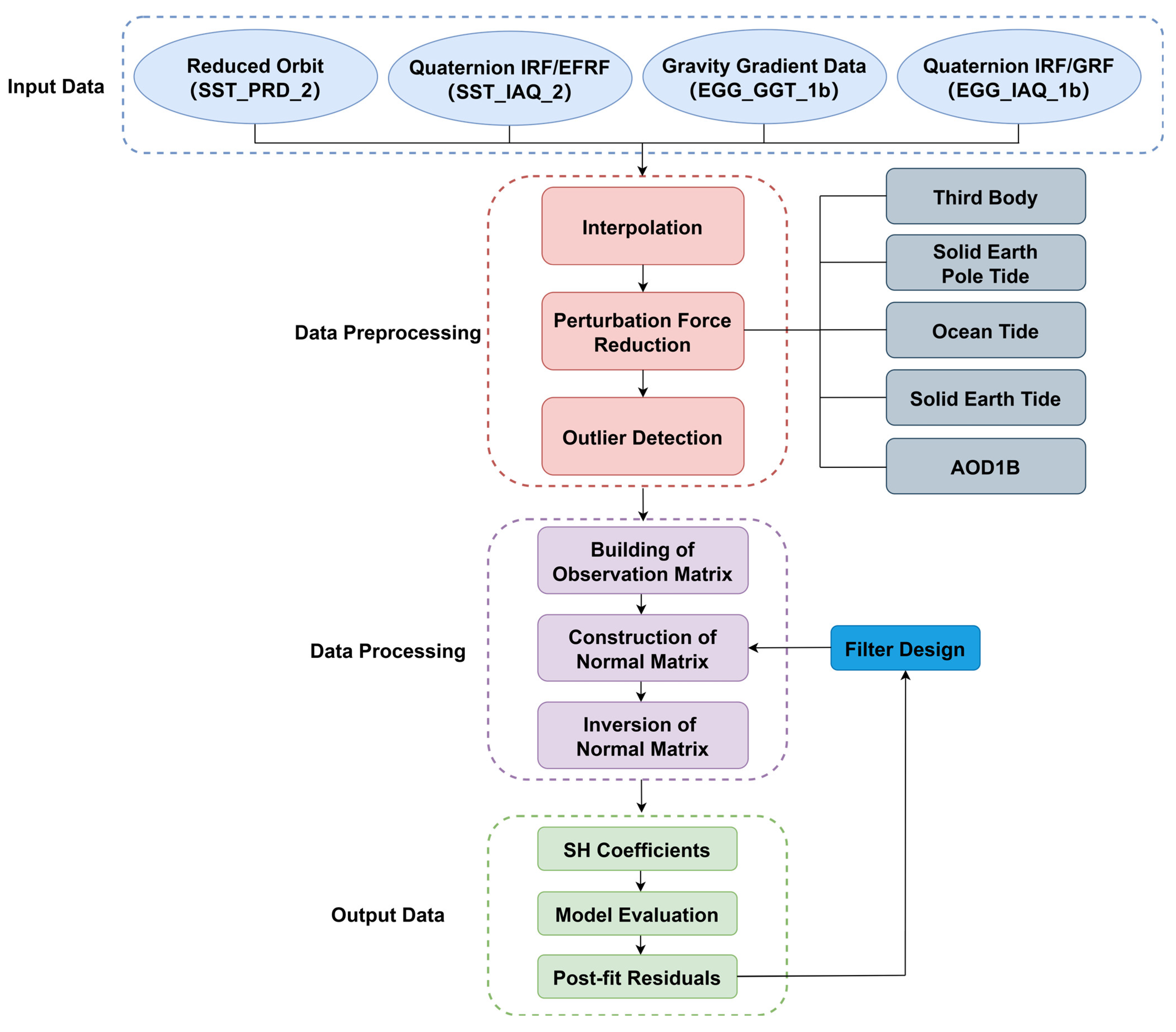
Figure 1 illustrates the processing flow of recovering a high-degree gravity field model based on the GOCE gradient data. It consists of four parts, i.e., input data, data preprocessing, data processing, and the accuracy evaluation of the model. Firstly, the initial sampling rate of the input dynamic orbit is 10 s, which needs to be interpolated to 1 s to synchronize with the gravity gradient data. Then, the raw gravity gradient data needs to go through preprocessing steps such as outlier detection and perturbation force deduction to ensure the high quality of the input observations [42]. Secondly, the observation equations are established, and a system of normal equations is formed based on the time-wise method. Finally, the gravity field model is solved, and its accuracy analysis is performed. In this section, the above four modules are discussed in detail.
It has been shown that even a small number of outliers involved in the final gravity field solution can adversely affect the estimation of the spherical harmonic coefficients [43]. Therefore, it is important to detect the outliers as accurately as possible and remove them from the original gravity gradient data. The common methods currently used to identify outliers in gravity gradient data are statistical methods, wavelet outlier detection algorithms [43], and so on. In this paper, we will use the statistical method with moving windows to identify coarse differences, i.e., the observed value minus the simulated value (OMC), by setting upper and lower thresholds in each moving window. According to Albertella, et al. [44], the signal-to-noise ratio of the observed values should be reduced so that the coarse differences will be more obvious. Therefore, in this paper, the residual gradient is used to replace the original gravity gradient observation for coarse difference detection, where the reference gradient is calculated from the EGM2008 model with a truncation degree of 250. The coarse difference value in a moving window of size can be defined as
where is the OMC gradient in the window, and and are the estimate of the mean and standard deviation of OMC in the same window. According to Equation (1), the detection of coarse epochs depends heavily on the settings of the parameters and . A smaller value of and can make the detection of outliers more sensitive, but the disadvantage is that some ephemerides with relatively high accuracy will also be removed. The common settings of are 1, 2, 4, 8, and 16 revolutions of the satellite around the Earth, where each revolution corresponds to 5400 s of observations. Based on a comparison of a set of tests with different settings of and , they are set to 4 and 1 revolutions, respectively, in this paper. These detected coarse epochs are removed from the observed time series to avoid any impact on the subsequent gravity field recovery.
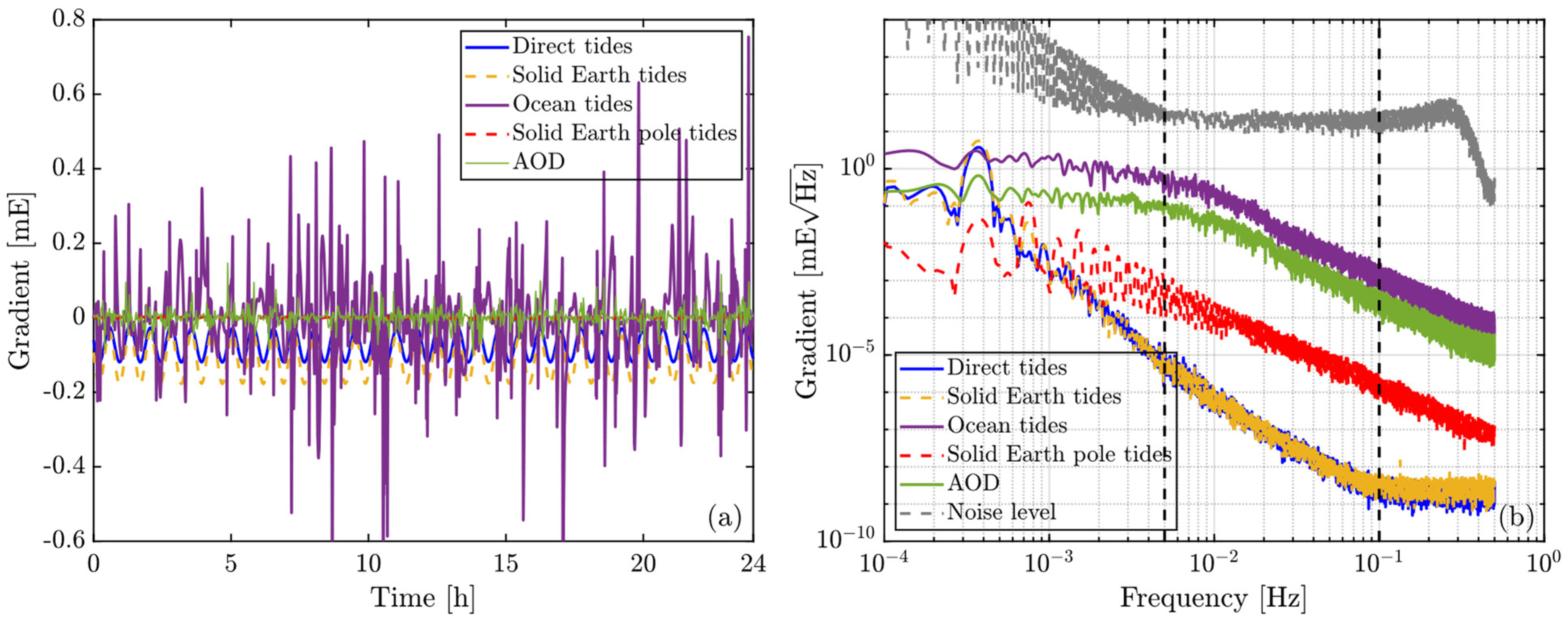
It is necessary to use the background model to make deductions before processing the gradiometer data since the latest version of the published data does not account for the influence of conservative forces such as the ocean tide and solid earth tide. The force models and observation data used in the solution process are shown in Table 1. We also displayed the calculated perturbation forces for the component as an example of one day in Figure 2.
The time-wise approach proposed by Pail, et al. [2] serves as the foundation for this paper’s analysis of the impact of various filter methods on the gravity field inversion. The partial derivative matrix of the gradient concerning the spherical harmonic coefficients of the gravity field and the reference gradient values are first calculated in the Earth-fixed Reference Frame (EFRF). Then, they are rotated to the Gradiometer Reference Frame (GRF) [45]. Next, the observation equation is established under the GRF as follows:
where is the design matrix, characterizing the relationship between the gradient observation and the spherical harmonic coefficient of the gravity field to be solved; is the gravity gradient observation of the GOCE satellite; is the observation error; is the normal gravity gradient under the GRF, which can be calculated by the normal gravity field.
According to Equation (2), the spherical harmonic coefficients of the gravity field model can be solved using the least squares adjustment:
where is the perturbed gravity gradient; is the variance–covariance matrix of the observations, and its reciprocal is used to weight the observations of each epoch.

Table 1.
Background force models and measurements.
| Force Model | Description |
|---|---|
| Static gravity field | TIM_R1 (Pail, et al. [2]; d/o = 224) |
| Ocean tide | EOT11a (Rieser, et al. [46]; d/o = 120) |
| Solid earth tide | IERS conventions (Petit, et al. [47]) |
| Solid earth pole tide | IERS conventions (Petit, et al. [47]) |
| Third body | DE421 (Folkner, et al. [48]) |
| AOD | AOD1B RL06 (Dobslaw, et al. [49]) |
| Dynamic orbit | Level 2, sampling rate 10 s |
| Gravity gradient | Level 1b, sampling rate 1 s |
| Attitude | Level 1b, sampling rate 1 s |
2.2. Filter Design
Assuming that the post-fit residuals of the observations are stationary [50], the variance–covariance matrix has a Toeplitz structure and can be calculated from the posterior residuals. However, as mentioned in the introduction, the dimension of the variance–covariance matrix will increase as the number of observations increases. This process will consume more computer memory to perform a direct statistical calculation of the covariance matrix. To improve the computational efficiency, the Cholesky decomposition of the variance–covariance matrix in Equation (2) is obtained as:
where denotes the Cholesky decomposition matrix. Substituting it into Equation (3) yields,
where
At this point, the variance–covariance matrix has the following relationship holding:
where is the unit matrix, implying that the ephemeris elements are independent of each other. The matrix plays a de-correlation role here and can be considered as a filter. In the specific solution, can be a single kind of filter or a combination of several filters (product of filters , and are each a single filter) for complex error characteristics. Schuh, et al. [30] developed a new method of constructing directly from the PSD of the posteriori residual, which further improves the computational efficiency while ensuring that the accuracy of the solution is not compromised. Therefore, this paper will also adopt this approach to construct the filter in the subsequent process of solving the gravity field.
In general, a discrete system (in this paper, a filter) with constant linear shift can be represented by a differential equation [30]:
where is the filtered time series; is the original time series, which in this paper corresponds to the posterior residuals; and are the filter coefficients, which can be estimated based on different types of filter algorithms. In this paper, we considered nine filter combinations to evaluate their influence on the gravity field model recovery, as depicted in Table 2. To facilitate the subsequent presentation of the paper, we use different characters to represent the corresponding filter combinations. in the equation is the order of the filter, which is generally determined by the AIC criterion [51]. Among them, the differential filter corresponds to the order (1, 1); the notch filter corresponds to the order (2, 2); the high-pass filter corresponds to the order (4, 4); the bandpass filter corresponds to the order (8, 8); and the empirical parameters are constructed according to the method mentioned in Section 3.3 of Kim, et al. [52]. For the selection of the frequency bandwidth, the BP1 is 5 mHz~100 mHz while the BP2 is related to the cut-off frequency, and the high pass filter is only considered for the signals after 1 cpr.
In this study, three sets of experiments are designed to effectively assess the influences of the above filters on the gravity field inversion based on the GOCE gravity gradient data. (1) To investigate the influence of low-frequency errors, six filters are considered when solving the gravity field model for BP1, BP2, DF, ARMA, DARMA, and HARMA, respectively. (2) Five cascade filters, DARMA, HARMA, DNARMA, DARMAL, and HARMAL, are taken into account to solve the gravity field model to analyze the impact of the orbital frequency error on the solution. (3) Based on the result of the above two sections, different filter estimation frequencies are chosen to investigate the effect of the stability of the observation error on the recovered results.
3. Results and Discussion
3.1. Effect of Different Filter Combinations on Gravity Field Inversion Results for Low-Frequency Errors
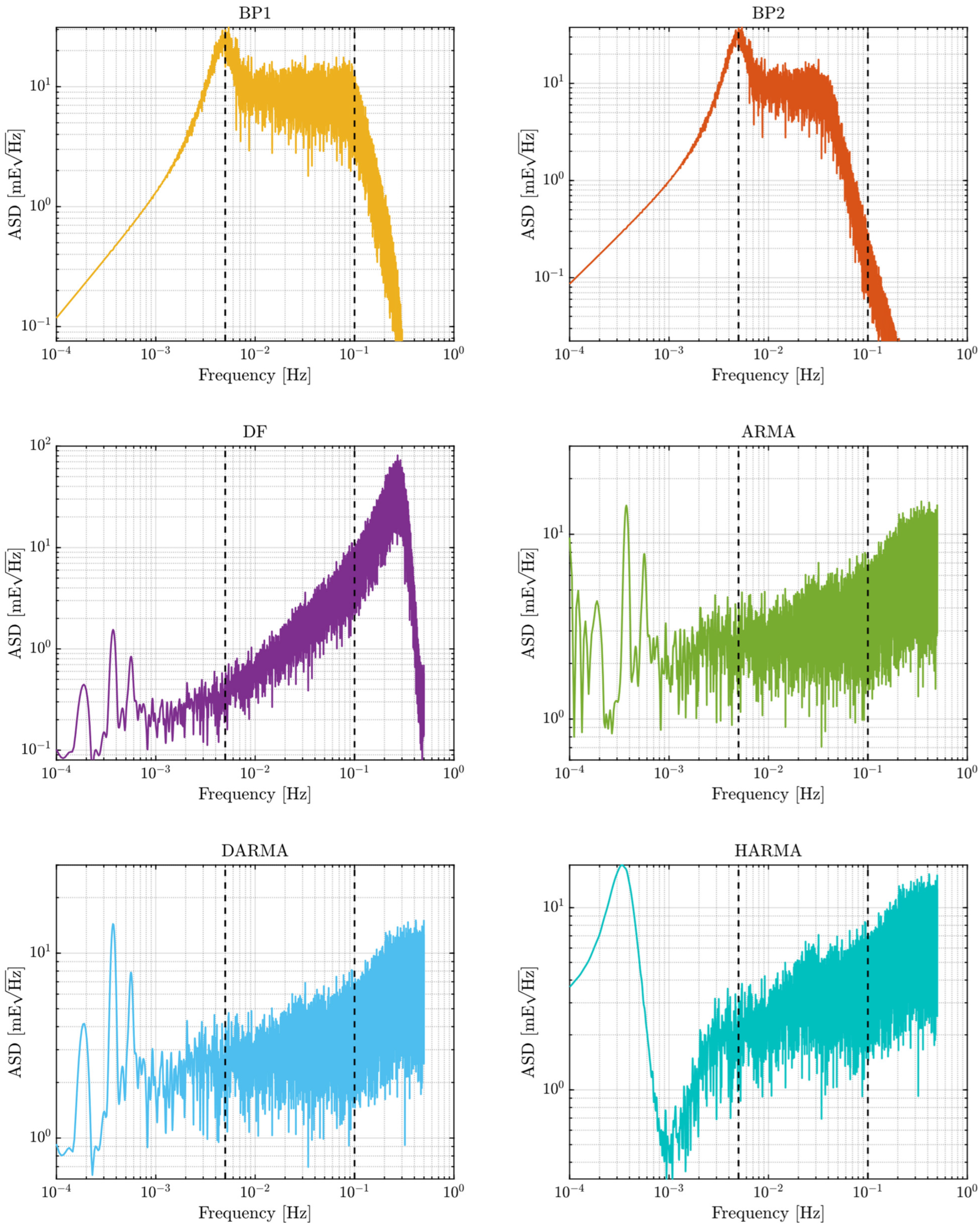
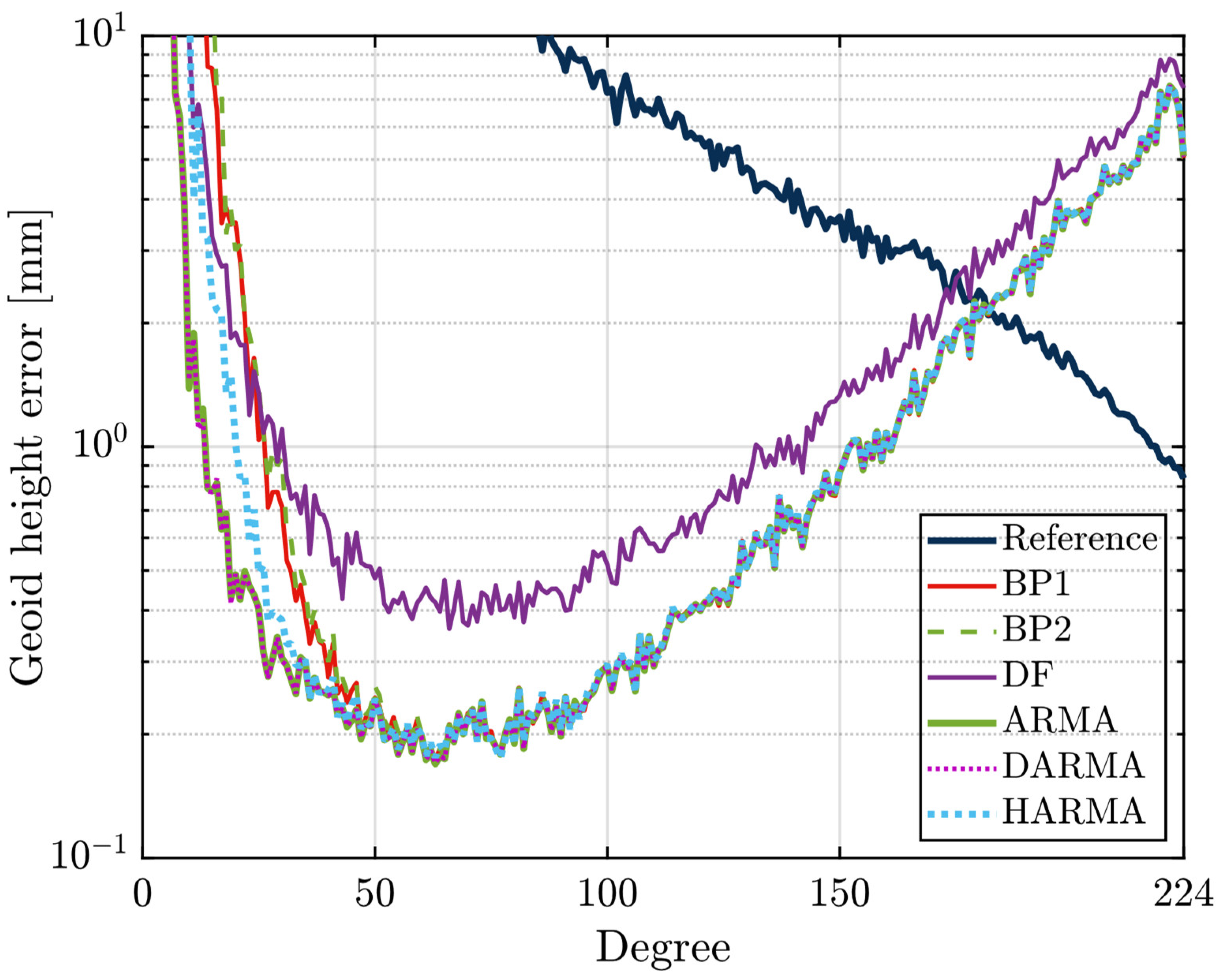
The observation error of the gradiometer, due to the electrostatic accelerometer’s drift phenomena, presents in the low-frequency section. This research initially investigates the effect of various filter combinations on the result of the gravitational field inversion for this type of error characteristic. The six filters BP1, BP2, DF, ARMA, DARMA, and HARMA in Table 2 were selected to process the observation noise of the GOCE satellite gradiometer. The filtered error curves of the observation errors are shown in Figure 3. Except for DF, the other five filter combinations can retain the observed signal within the MBW (that is 5 mHz~100 mHz for GOCE gradient data). The differences are that the two filters of ARMA and DARMA can maximize the signal in the whole observation band, while the other two filters BP1 and BP2 completely filter out the signal and noise in the low-frequency part. The DF suppresses the noise in the low-frequency region while filtering out the observation signal in the MBW. Substituting the above six filters into Equation (5), the gravity field spherical harmonic coefficients are solved. The degree error RMS of geoid height is then calculated using Equation (10) after the difference with the reference model has been calculated. The results are displayed in Figure 4, where the reference gravity field model is the TIM_R1 model [3].
where and are the solved spherical harmonic coefficients, while and are the spherical harmonic coefficients of the reference gravity field model, n and m are the degree and order of the gravity field model, respectively, and is the mean radius of the Earth.
The results reveal that each filtering algorithm is not entirely compatible from 2 to 50 d/o, and the solution of the other five filter combinations are consistent after 50 d/o, the except for the DF. And in the further step, BP1 and BP2 have the worst computational accuracy, which is related to the characteristics of the bandpass filter itself, which retains the signal within MBW to the maximum while filtering out the noise outside MBW. The benefit of this design is that it improves the computational speed and allows the results to be obtained without iterations. Nevertheless, the low-frequency portion of the signal is also filtered out along with the noise outside the MBW, resulting in poor accuracy of the final solution results in the low-frequency part. In contrast, ARMA and DARMA perform better in the low-degree part since the ARMA is a full-frequency band whitening filter that finely suppresses the low-frequency error. From 2 to 20 d/o, the solution accuracy of DF is superior to BP1 and BP2. However, the accuracy of this filter decreases as the degree rises after 20 d/o, and the accuracy after 50 d/o is the poorest. It is so that the filtering algorithm achieves the de-correlation by directly differencing adjacent epochs, which suppresses the low-frequency error while distorting the high-frequency part. The cascade filter HARMA is composed of an ARMA filter and a high-pass filter. The low-frequency error is first reduced by employing a high-pass filter, and the ARMA filter is then constructed based on the filtered residuals. The low-frequency error will be filtered out simultaneously by the high-pass filter with a truncation effect, preventing this filter combination from having the same effect as ARMA and DARMA while still maintaining the realistic gravity field signal of the high-degree region.
To further investigate the impacts of the above six filters on the different degrees of the gravity field, we divided each model into five intervals by degree (2~10, 11~20, 21~50, 51~224, and 2~224) and calculated the cumulative degree variance within each interval by Equation (11). Table 3 presents the statistical result.
where and are the interval values, and are the solved spherical harmonic coefficients, while and are the spherical harmonic coefficients of the reference gravity field model, n and m are the degree and order of the gravity field model, respectively, and is the mean radius of the Earth.
In addition to the previous conclusions, the analysis of the results reveals that: (1) Although both BP1 and BP2 utilized bandpass filters, BP1’s total cumulative error is 25% lower than BP2’s due to different cutoff frequencies. The filter cutoff frequency of BP2 is related to the maximum degree of solution [38], conforming to the relationship: , where is the cutoff frequency, is the satellite orbital period, and is the maximum degree of the gravity field. In contrast, BP1 retains the signal in the 5~100 MHz bandwidth. Further analysis of the cumulative errors in the five intervals shows that the differences between BP1 and BP2 are mainly concentrated in the interval from 2 to 10, and the solution accuracy of the two is relatively close in the other four intervals, indicating that both filtering algorithms retain the signal in the MBW well. However, the differences in the low-frequency part show that the gravity field d/o and the frequency of the observed data are not clearly one-to-one correspondence. The signal outside the cutoff frequency considered by BP1 also contributes to the solution of the low-frequency part, which makes its solution results more accurate in the low-frequency region compared to BP2. This also supports the conclusion of [54]. (2) Two filtering algorithms, ARMA and DARMA, showed the greatest improvement in accuracy. In particular, the DARMA filter has the highest accuracy thanks to its integrated consideration of colored noise in the low-frequency part and the full-frequency band. It reduces the total cumulative error by 96.087% relative to BP2. The discrepancies between ARMA, DARMA, and BP2 are primarily focused on the 2~50 d/o, which further confirms the efficiency of the ARMA filter in handling low-frequency errors, according to an assessment of the cumulative errors in five intervals. (3) When comparing the total cumulative error, DF’s solution accuracy is second only to ARMA and DARMA, which is reduced by 95.7% compared to BP2. However, the lower total cumulative error of DF is attributable to its superior accuracy in two intervals from 2 to 10 and 11 to 20, as can be shown by examining the cumulative error in each period. It has larger cumulative errors than the other filters in two intervals from 21~50 and 51~224. This is consistent with the fact that the degree error RMS of the geoid height of DF in Figure 1 is the largest in the higher degree part.
From the above analysis, it can be concluded that two filtering algorithms, ARMA and DARMA, are suggested for processing the GOCE gradient data to ensure the maximum preservation of the observed signal in the low-frequency region while subtracting the low-frequency error. This is also in line with the conclusion reached by Schuh, et al. [32] after comparing four filters.
3.2. Effect of Different Filter Combinations on Inversion Results for Orbital Frequency Errors
In addition to the characteristic in the low-frequency part, the gradient observation error is frequently superimposed by the accelerometer error and the background model noise with the orbital frequency error [29]. Siemes, et al. [34] proposed to filter the orbital frequency error by using a notch filter for the error characteristic, which can play a good role in suppressing it. However, in practical applications, the filter requires a long data segment for warming up, which leads to many missing observations and reduces computational efficiency. A more common approach is to absorb the noise at the orbital frequency by introducing empirical parameters [52]. According to the experimental findings, this strategy can significantly improve the accuracy of the gravity field. So, we will take the 1 cpr error as an example to explore the implications of various filter combinations for the orbital frequency error in this section.
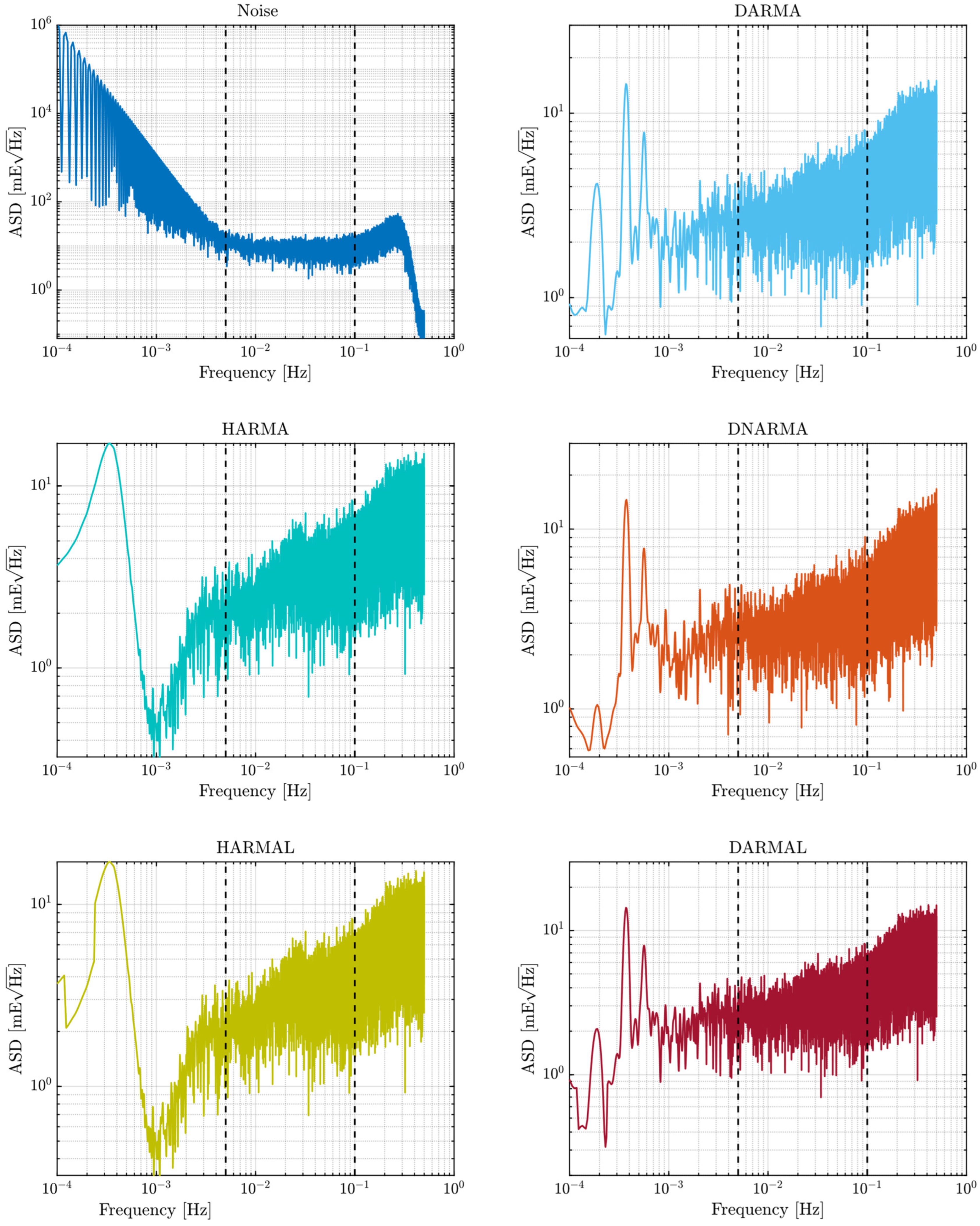
Consistent with the analysis method in Section 3.1, the five filters DARMA, HARMA, DNARMA, DARMAL, and HARMAL in Table 2 are chosen to process the observation noise of the GOCE satellite gradiometer. The error curves of the observation errors before and after filtering are displayed in Figure 5. The filter combinations of DARMA, DNARMA, and DARMAL perform relatively better, and all of them can retain the observed signal in the whole observation band. Compared with DARMA, the amplitude of the filtered time series decreases to a certain extent at 1 cpr after the introduction of empirical parameters or notch filter (DARMAL or DNARMA).
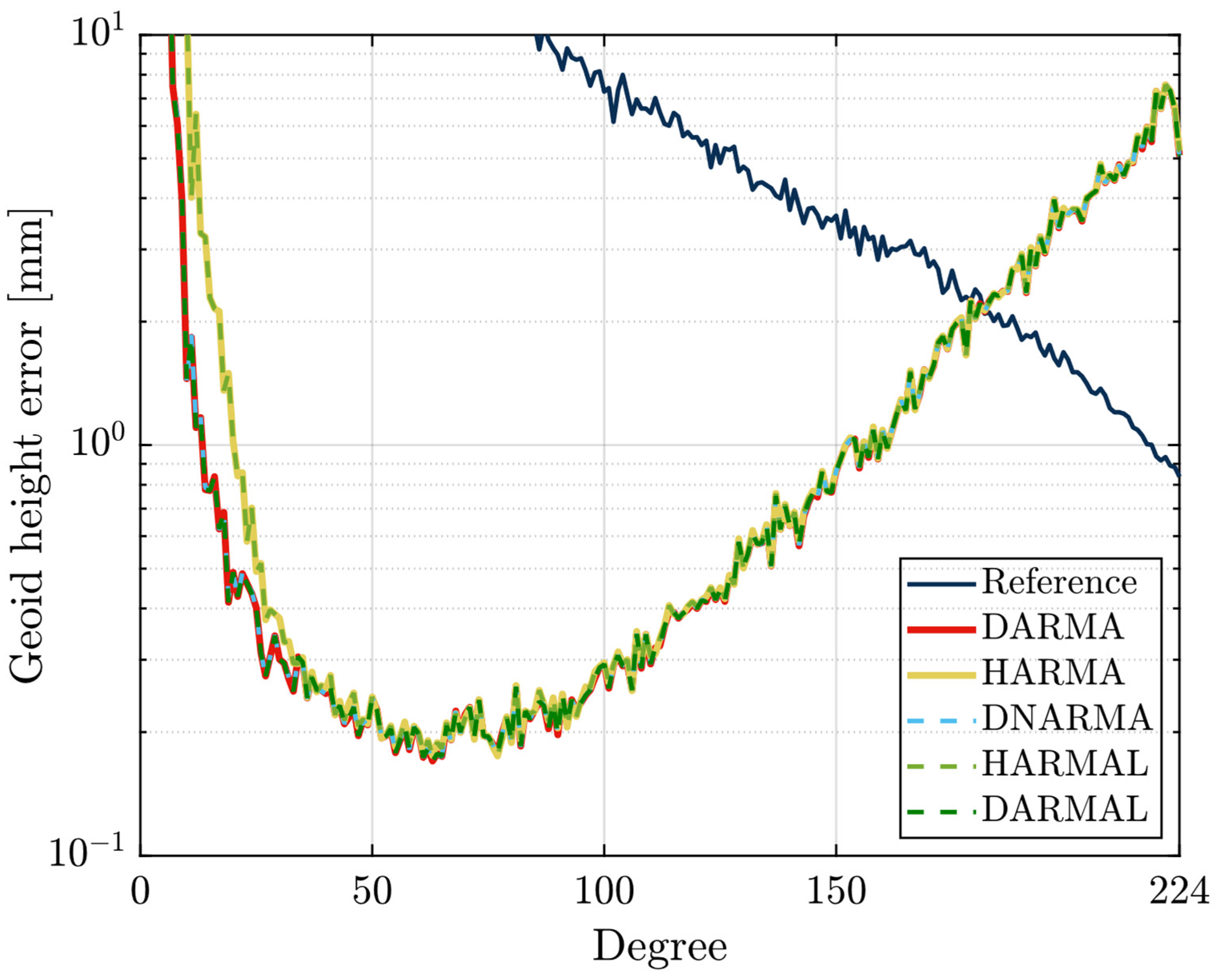
The gravity field models are solved based on the above five filters and the corresponding degree error RMS of the geoid height is calculated. The results are shown in Figure 6. The effect of introducing empirical parameters or notch filters on the basis of DARMA or HARMA is not very well represented in the degree variance curves.
To further analyze the role of empirical parameters and notch filters, five intervals were separated for each model using the same criteria as in Section 3.1, and the cumulative degree error RMS of geoid height within each interval was calculated. The results are displayed in Table 4 to further evaluate the effects of various filter combinations on different degrees. It can be found that the differences between HARMA (or HARMAL) and the other three filter combinations are mainly represented in the two intervals from 2~10 d/o and 11~20 d/o. The cumulative degree error RMS of geoid height in the remaining two intervals is relatively close, and the maximum does not exceed 2 mm.
DNARMA, using a notch filter to eliminate the effect of octave error, and DNARMA are comparable in terms of cumulative degree variance across all intervals, with 2~10 showing the most significant difference. Since the orbit frequency error can only be approximated slowly by iterative calculation during filter design, the orbit frequency error is eliminated by the notch filter while absorbing part of the signal. Therefore, the accuracy of the final solution will directly depend on the precision of the orbit frequency error estimation when applying the notch filter.
In contrast to DNARMA, DARMAL is built based on Kim. [52] proposal for an empirical parameter technique to reduce the impact of orbit frequency error. DARMAL has higher accuracy compared with DNARMA and DARMA, demonstrating that the addition of empirical parameters can eliminate the influence of orbit frequency errors to a certain extent. However, the accuracy of the low-frequency region was not improved by empirical parameters based on HARMAL, and the inaccuracy increased in the range of 2~10 d/o. The possible reason is that the addition of empirical parameters after filtering out the signal and noise below the 1 cpr part with a high pass filter will further make the results worse.
Through the above comparison, it can be concluded that the filter combination DARMAL is the best option for dealing with low-frequency errors and orbital frequency errors. Nevertheless, the total cumulative degree variance is only improved by 0.5 mm compared to the DARMA filter combination. As a result, there are increased demands on computer space and processing speed. Given the accuracy of the solution and the efficiency of the calculation, it is suggested to employ the DARMA filter algorithm.
3.3. Effect of Error Stability on Inversion Results
The premise of the above filter construction is to ensure that the GOCE gradient error is stationary. However, the observations are frequently not divided into relatively short arc lengths because the filter needs warming up in the actual calculation, making it challenging to determine whether the error within each arc segment is steady state. Brockmann, et al. [4] separated the observations into various arc segments according to the gradient data intermittent ephemeris when recovering the gravity field. As a result, the arc lengths were not uniform, with some arcs containing several months of data and others including only a few days of data. In the subsequent filter design, the errors within each arc were considered a stable condition, and the filter was estimated separately. Nonetheless, GOCE satellites are subject to satellite re-orbiting and the influence of the observation environment throughout the mission, which may lead to non-stationary gradient observation errors within a complete data segment. If a band-pass filter is employed in this situation to deal with the observation error, the non-stationary nature of the error will not affect the solution results. It, however, has an impact on the data processing, and, consequently, the accuracy of the inversion results if a cascade filter is employed to decorrelate the colored noise. This part will discuss the implication of various filter estimation frequencies on the recovered results to address this issue.
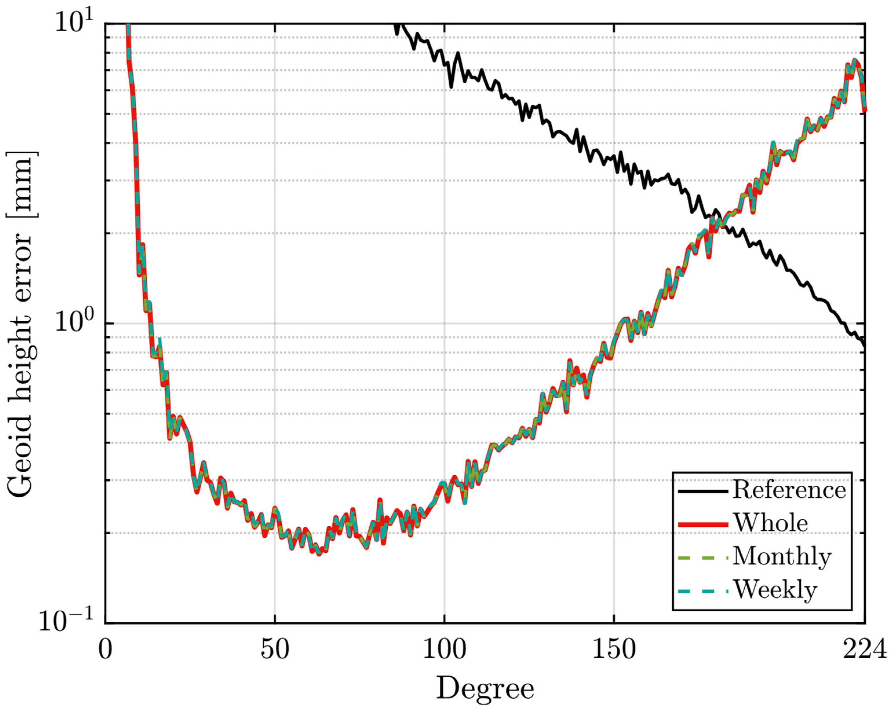
In the section, the DARMA filter is estimated for three arc lengths of 72 days, 36 days, and 7 days, respectively, taking a total of 72 days of data segments from 1 November 2009 to 11 January 2010, as an example. The gravity field model was then solved using Equation (5), and the degree error RMS of geoid height was determined using Equation (10). As shown in Figure 7, the new version of the gradient data (0202) is not sensitive to the filters estimated by the three arc lengths, and the accuracy of the solution results is extremely similar. All degrees are split into five intervals so that the effects of various filter estimation durations on various degrees can be further investigated. Equation (11) is used to compute the cumulative degree error RMS of geoid height across different intervals, and the results are displayed in Table 5. The statistical results demonstrate that the three estimated periods in each interval’s cumulative degree variances are rather near to one another, with a maximum not surpassing 0.4%. It implies that the GOCE satellite error for the new version of gradient data is stationary during the whole data period.
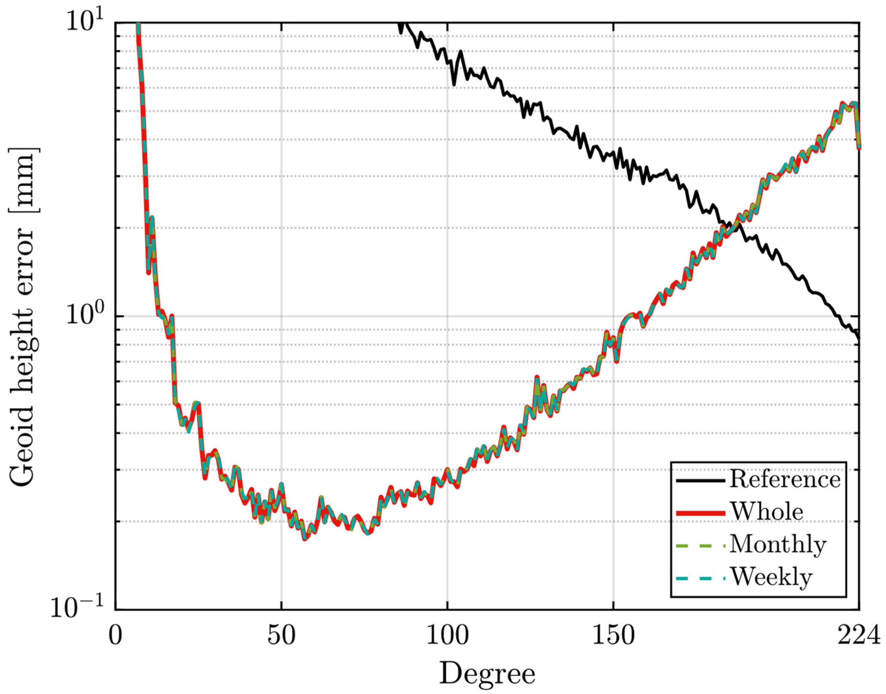
This work also chose a data segment from the 62 days of data collected between 10 November 2012 and 10 January 2013 which was detected by the continual orbital de-orbiting in the late part of the satellite mission to better verify the above conclusions. Similarly, the three arc segment lengths of 62 days, 31 days, and 7 days are selected based on the observed data of this data segment to estimate the DARMA filter. The gravity field model and the related degree error RMS of geoid height for the three periods are calculated, and the results are shown in Figure 8. It can be seen from the figure that the new version of data is equally insensitive to different estimation periods compared with the previous data segment, and the three inversion results are better conformed in the full frequency band. To further analyze the effect of the three filter estimation periods on the different orders of the new version of the data, the full frequency band was divided into five intervals using the same division criteria as in Section 3.1, and the cumulative degree error RMS of geoid height of each interval was calculated according to Equation (11), as shown in Table 6. It is clear from the figure that the new version is similarly insensitive to different estimation periods, and the three inversion results are conformed in the entire frequency band. The cumulative degree error RMS of the geoid height of each interval shows that the new version of the data is relatively close to each other, and the maximum does not exceed 3 mm, which also reveals that the observation errors in the new version of the data are stable and not affected by factors such as satellite orbit adjustment.
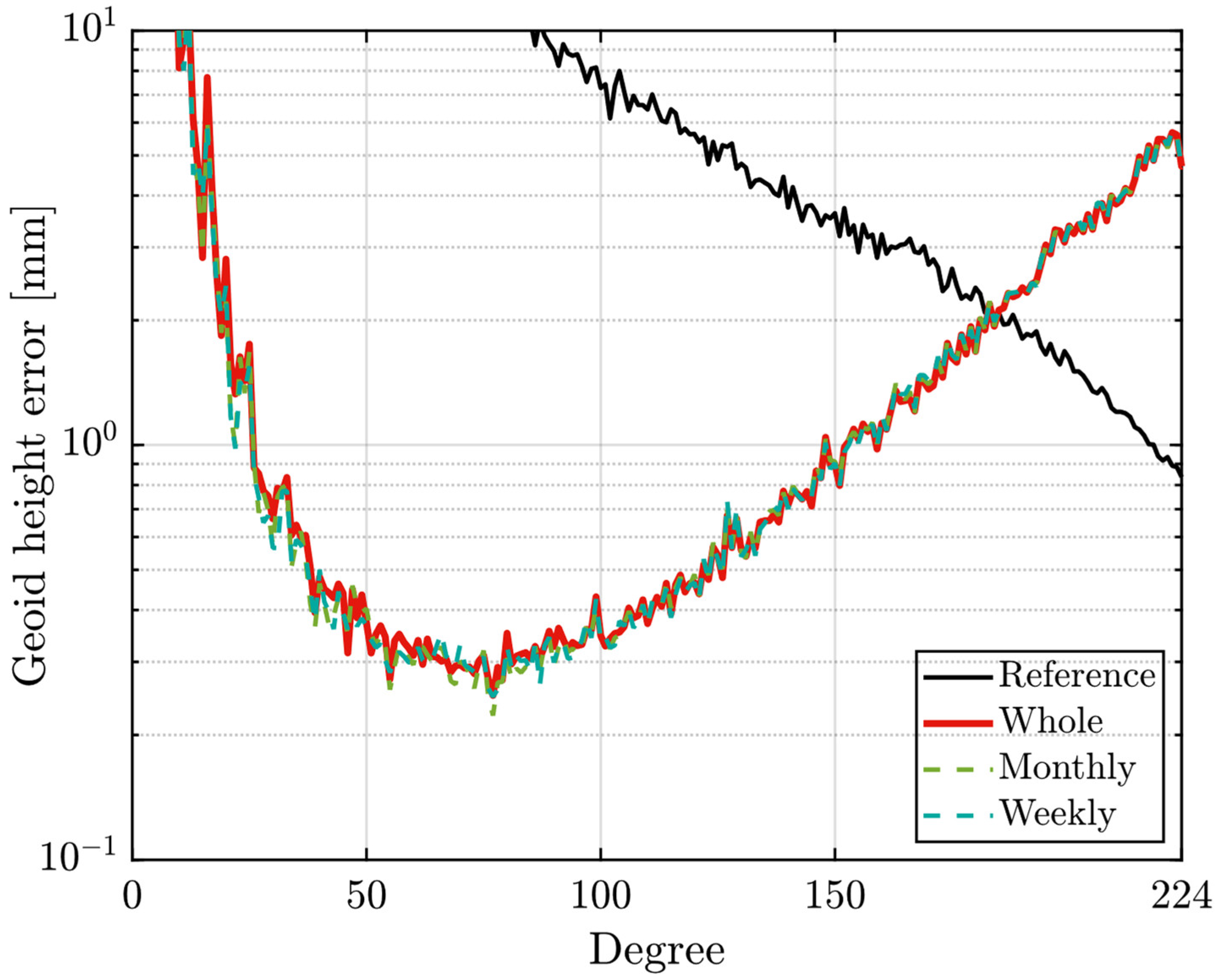
In addition, the old version of the same data segment (0103) was selected for comparison. The results in Figure 9 show that the low-frequency portion of the old version of this data segment is somewhat sensitive to various filter estimation periods. Moreover, the entire frequency band was divided into five intervals using the same division criteria as in Section 3.1, and the corresponding cumulative degree error RMS of geoid height was calculated according to Equation (11). The statistical results in Table 7 show that the solution solved based on the old version of the data has the highest accuracy when the estimation filter is weekly applied, and the errors are reduced by 10 cm and 3 cm, respectively, compared with those by the full-arc and monthly estimation filters. The improvement is primarily localized in the low-frequency parts, indicating that the satellite observation environment mainly affects the low-frequency areas of the observed data, and has less influence on the signal in the MBW. It also verifies that the updated processing procedure has improved the accuracy of the observation data as well as the stability of the observation error.
We can infer from the above study that the factor of the non-stationary characteristic of observation error can be ignored when solving the gravity field using the new version of data. It is feasible to estimate the filters based on the length of data interruptions and solve the gravity field model in segments to optimize computing efficiency. Choosing alternative arcs to build filters based on the satellite’s observation environment is required for the older version of the data. The filter can be determined by dividing the arc segments according to the data interruptions if the observation environment is steady across the period and the accuracy can meet the necessary standards. It is advised to estimate the filter weekly if the satellite’s observation environment is unstable during the observation period and there are instances where the orbit is lifted or lowered.
4. Conclusions
This paper examines the performance of different filter combinations in handling the error in the low-frequency part of the gradient data, the orbital frequency error, and the error stability. A total of nine filter algorithms, including band-pass filter, differential filter, ARMA filter, notch filter, and combined filter constructed by combining different filters, are selected by considering the existing filter algorithms.
According to the experimental results, the cascaded filter (DARMA), consisting of a differential filter and an ARMA filter, has the best accuracy because it can whiten the data across the whole band while considering the low-frequency error. For dealing with orbital frequency errors, the addition of the notch filter worsens the solution. It is because the notch filter is empirical-based and designed totally, which does not accurately reflect the magnitude of the multiplication error and leads to a decrease in the accuracy of the inversion results. We suggest selecting the DARMA filter combination for the real solution based on the consideration of computational efficiency. Finally, the influence of the error stability characteristics on the filter estimation and the gravity field solution is discussed by using the DARMA filter as an example. The analysis reveals that the old version of the gradient data is more sensitive to the satellite observation environment. For data segments with a high frequency of satellite operations, it is recommended to estimate the filter by week when solving for the gravity field solution. In contrast, the enhanced calibration method for the current version of the data has extensively addressed the non-stationary characteristics. Therefore, the impact of the satellite environment can be neglected, and estimating the filter from intermittent data is entirely feasible.
Due to the availability of the updated data in 2019, many research institutions may update their solution models in the future. Based on the findings of this article, it is suggested that the DARMA filters are estimated separately by dividing the arcs of the data intermittently for solving the high-precision geostationary gravity field models in the specific calculation. It ensures the solution’s accuracy and maximizes the efficiency calculation. Furthermore, it is worth noting that the presence of outliers not only directly affects the solution, but also the filter estimating process. Therefore, the coarse epochs should be handled more finely during the data preprocessing procedures.
Author Contributions
Conceptualization, Q.M.; methodology, Q.M.; software, Q.M.; validation, L.L. and Y.Y.; writing—original draft preparation, Q.M.; writing—review and editing, C.W., L.L., Y.Y. and M.Z.; visualization, Q.M.; supervision, M.Z.; funding acquisition, C.W., L.L. and M.Z. All authors have read and agreed to the published version of the manuscript.
Funding
This research was funded by the National Natural Science Foundation of China (Grants No. 42174103, No. 12261131504, No. 42027802, and No. 42204091), the National Key R&D Program of China (Grant No. 2022YFC2204601), the Open Fund of Hubei Luojia Laboratory (Grant No. 220100044).
Data Availability Statement
The GOCE L1B data are downloaded from the European Space Agency (ESA).
Acknowledgments
Thanks to the valuable comments given by the anonymous reviewers, which are so helpful for the improvement of the text, figures, and other related contents of this paper. We are grateful to the European Space Agency for providing the GOCE L1B data, to the China Scholarship Council CSC for funding Qinglu Mu’s research work in Germany, and to Weiyong Yi for his valuable comments on specific calculation details.
Conflicts of Interest
The authors declare no conflict of interest.
References
- European Space Agency. Gravity Field and Steady-State Ocean-Circulation Mission, Report for Mission Selection of the Four Candidate Earth Explorer Missions; Tech. Rep. 1999, ESA SP-1233; ESA Publications Division: Noordwijk, The Netherlands, 1999. [Google Scholar]
- Pail, R.; Goiginger, H.; Mayrhofer, R.; Schuh, W.D.; Brockmann, J.M.; Krasbutter, I.; Fecher, T. GOCE gravity field model derived from orbit and gradiometry data applying the time-wise method. In Proceedings of the ESA Living Planet Symposium, Bergen, Norway, 28 June–2 July 2010; ESA Publication: Noordwijk, The Netherlands, 2010; p. SP-686. [Google Scholar]
- Pail, R.; Bruinsma, S.; Migliaccio, F.; Förste, C.; Goiginger, H.; Schuh, W.D.; Tscherning, C.C. First GOCE gravity field models derived by three different approaches. J. Geod. 2011, 85, 819–843. [Google Scholar]
- Brockmann, J.M.; Zehentner, N.; Höck, E.; Pail, R.; Loth, I.; Mayer-Gürr, T.; Schuh, W.D. EGM_TIM_RL05: An independent geoid with centimeter accuracy purely based on the GOCE mission. Geophys. Res. Lett. 2014, 41, 8089–8099. [Google Scholar]
- Brockmann, J.M.; Schubert, T.; Schuh, W.D. An improved model of the Earth’s static gravity field solely derived from reprocessed GOCE data. Surv. Geophys. 2021, 42, 277–316. [Google Scholar]
- Bruinsma, S.; Marty, J.C.; Balmino, G.; Biancale, R.; Förste, C.; Abrikosov, O.; Neumayer, H. GOCE gravity field recovery by means of the direct numerical method. In Proceedings of the 2010 ESA Living Planet Symposium, Bergen, Norway, 28 June-2 July 2010. [Google Scholar]
- Bruinsma, S.L.; Förste, C.; Abrikosov, O.; Marty, J.C.; Rio, M.H.; Mulet, S.; Bonvalot, S. The new ESA satellite-only gravity field model via the direct approach. Geophys. Res. Lett. 2013, 40, 3607–3612. [Google Scholar]
- Bruinsma, S.L.; Förste, C.; Abrikosov, O.; Lemoine, J.M.; Marty, J.C.; Mulet, S.; Bonvalot, S. ESA’s satellite-only gravity field model via the direct approach based on all GOCE data. Geophys. Res. Lett. 2014, 41, 7508–7514. [Google Scholar] [CrossRef]
- Migliaccio, F.; Reguzzoni, M.; Gatti, A.; Sansò, F.; Herceg, M. A GOCE-only global gravity field model by the space-wise approach. In Proceedings of the 4th International GOCE User Workshop, Munich, Germany, 31 March–1 April 2011. [Google Scholar]
- Farahani, H.H.; Ditmar, P.; Klees, R.; Liu, X.; Zhao, Q.; Guo, J. The static gravity field model DGM-1S from GRACE and GOCE data: Computation, validation and an analysis of GOCE mission’s added value. J. Geod. 2013, 87, 843–867. [Google Scholar]
- Wu, H.; Müller, J.; Brieden, P. The IfE global gravity field model from GOCE-only observations. In Proceedings of the International Symposium on Gravity, Geoid and Height Systems, Thessaloníki, Greece, 19–23 September 2016. [Google Scholar]
- Schall, J.; Eicker, A.; Kusche, J. The ITG-Goce02 gravity field model from GOCE orbit and gradiometer data based on the short arc approach. J. Geod. 2014, 88, 403–409. [Google Scholar]
- Yi, W. An alternative computation of a gravity field model from GOCE. Adv. Space Res. 2012, 50, 371–384. [Google Scholar]
- Xu, X.; Zhao, Y.; Reubelt, T.; Tenzer, R. A GOCE only gravity model GOSG01S and the validation of GOCE related satellite gravity models. Geod. Geodyn. 2017, 8, 260–272. [Google Scholar]
- Chen, J.; Zhang, X.; Chen, Q.; Liang, J.; Shen, Y. Unconstrained gravity field model Tongji-GOGR2019S derived from GOCE and GRACE data. Chin. J. Geophys. 2020, 63, 3251–3262. [Google Scholar]
- Zhong, B.; Luo, Z.; Li, J.; Wang, H. Spectral combination method for recovering the Earth’s gravity field from High-low SST and SGG data. Acta Geod. Cartogr. Sin. 2012, 41, 735–742. [Google Scholar]
- Yu, J.; Wan, X. Recovery of the gravity field from GOCE data by using the invariants of gradient tensor. Sci. China Earth Sci. 2013, 56, 1193–1199. [Google Scholar] [CrossRef]
- Lu, B.; Luo, Z.; Zhong, B.; Zhou, H.; Flechtner, F.; Förste, C.; Zhou, R. The gravity field model IGGT_R1 based on the second invariant of the GOCE gravitational gradient tensor. J. Geod. 2018, 92, 561–572. [Google Scholar] [CrossRef]
- Rummel, R. Earth’s gravity from space. Rend. Lincei. Sci. Fis. E Nat. 2020, 31, 3–13. [Google Scholar] [CrossRef]
- Rio, M.H.; Mulet, S.; Picot, N. Beyond GOCE for the ocean circulation estimate: Synergetic use of altimetry, gravimetry, and in situ data provides new insight into geostrophic and Ekman currents. Geophys. Res. Lett. 2014, 41, 8918–8925. [Google Scholar] [CrossRef]
- Fuchs, M.J.; Bouman, J.; Broerse, T.; Visser, P.; Vermeersen, B. Observing coseismic gravity change from the Japan Tohoku-Oki 2011 earthquake with GOCE gravity gradiometry. J. Geophys. Res. Solid Earth 2013, 118, 5712–5721. [Google Scholar] [CrossRef]
- Ebbing, J.; Haas, P.; Ferraccioli, F.; Pappa, F.; Szwillus, W.; Bouman, J. Earth tectonics as seen by GOCE-Enhanced satellite gravity gradient imaging. Sci. Rep. 2018, 8, 16356. [Google Scholar] [CrossRef]
- Bingham, R.J.; Haines, K.; Lea, D. A comparison of GOCE and drifter-based estimates of the North Atlantic steady-state surface circulation. Int. J. Appl. Earth Obs. Geoinf. 2015, 35, 140–150. [Google Scholar] [CrossRef]
- Álvarez, O.; Gimenez, M.; Folguera, A. Analysis of the coseismic slip behavior for the MW = 9.1 2011 Tohoku-Oki earthquake from satellite GOCE vertical gravity gradient. Front. Earth Sci. 2022; 10, 1068435. [Google Scholar]
- Becker, S.; Brockmann, J.M.; Schuh, W.D. Mean dynamic topography estimates purely based on GOCE gravity field models and altimetry. Geophys. Res. Lett. 2014, 41, 2063–2069. [Google Scholar] [CrossRef]
- Dufréchou, G.; Martin, R.; Bonvalot, S.; Bruinsma, S. Insight on the western Mediterranean crustal structure from GOCE satellite gravity data. J. Geodyn. 2019, 124, 67–78. [Google Scholar] [CrossRef]
- Michaelis, I.; Styp-Rekowski, K.; Rauberg, J.; Stolle, C.; Korte, M. Geomagnetic data from the GOCE satellite mission. Earth Planets Space 2022, 74, 135. [Google Scholar] [CrossRef]
- Frommknecht, B.; Lamarre, D.; Meloni, M.; Bigazzi, A.; Floberghagen, R. GOCE level 1b data processing. J. Geod. 2011, 85, 759–775. [Google Scholar] [CrossRef]
- Rummel, R. Preface to the special issue on “GOCE-The Gravity and Steady-state Ocean Circulation Explorer”. J. Geod. 2011, 85, 747. [Google Scholar] [CrossRef]
- Schuh, W.D. Tailored Numerical Solution Strategies for the Global Determination of the Earth’s Gravity Field. In Mitteilungen der geodätischen Institute der Technischen Universität Graz; TU Graz: Graz, Austria, 1906; Volume 81. [Google Scholar]
- Schuh, W.D. The processing of band-limited measurements; filtering techniques in the least squares context and in the presence of data gaps. Space Sci. Rev. 2003, 108, 67–78. [Google Scholar] [CrossRef]
- Schuh, W.D.; Brockmann, J.M.; Kargoll, B.; Krasbutter, I.; Pail, R. Refinement of the stochastic model of GOCE scientific data and its effect on the in-situ gravity field solution. In Proceedings of the ESA Living Planet Symposium, Bergen, Norway, 28 June–2 July 2010; ESA Publication: Noordwijk, The Netherlands, 2010; p. SP-686. [Google Scholar]
- Klees, R.; Ditmar, P.; Broersen, P. How to handle colored observation noise in large least-squares problems. J. Geod. 2003, 76, 629–640. [Google Scholar] [CrossRef]
- Siemes, C. Digital Filtering Algorithms for Decorrelation within Large Least Squares Problems; IGG: Bonn, Germany, 2012. [Google Scholar]
- Zhu, G.; Chang, X.; Fu, X.; Qu, Q. A method for constructing the optimal ARMA filtering model on the satellite gravity gradiometry data. Chin. J. Geophys. 2018, 61, 4729–4736. [Google Scholar]
- Zhou, H.; Chuang, X.; Luo, Z.; Zhou, Z.; Zhong, B.; Wan, J. HUST-GOGRA2018s: A new gravity field model derived from the combination of GRACE and GOCE data. TAO: Terrestrial, Atmospheric and Oceanic Sciences. TAO Terr. Atmos. Ocean. Sci. 2019; 30, 9. [Google Scholar]
- Liu, T.; Zhong, B.; Li, X.; Tan, J. Filter design and comparison of gravity field inversion from GOCE satellite gravity gradient data. Geomat. Inf. Sci. Wuhan Univ. 2023, 48, 694–701. [Google Scholar]
- Wan, X.Y.; Yu, J.H.; Zeng, Y.Y. Frequency analysis and filtering processing of gravity gradients data from GOCE. Chin. J. Geophys. 2012, 55, 2909–2916. [Google Scholar] [CrossRef]
- Pitenis, E.; Mamagiannou, E.; Natsiopoulos, D.A.; Vergos, G.S.; Tziavos, I.N.; Grigoriadis, V.N.; Sideris, M.G. FIR, IIR and Wavelet Algorithms for the Rigorous Filtering of GOCE SGG Data to the GOCE MBW . Remote Sens. 2022; 14, 3024.40. [Google Scholar]
- Siemes, C.; Rexer, M.; Schlicht, A.; Haagmans, R. GOCE gradiometer data calibration. J. Geod. 2019, 93, 1603–1630. [Google Scholar] [CrossRef]
- Schubert, T.; Korte, J.; Brockmann, J.M.; Schuh, W.D. A generic approach to covariance function estimation using ARMA-models. Mathematics 2020, 8, 591. [Google Scholar] [CrossRef]
- Kern, M.; Preimesberger, T.; Allesch, M.; Pail, R.; Bouman, J.; Koop, R. Preprocessing of gravity gradients at the GOCE high-level processing facility. J. Geod. 2009, 83, 659. [Google Scholar]
- Albertella, A.; Migliaccio, F.; Sanso, F.; Tscherning, C.C. Outlier detection algorithms and their performance in GOCE gravity field processing. J. Geod. 2005, 78, 509–519. [Google Scholar]
- Albertella, A.; Migliaccio, F.; Sanss, F.; Tscherning, C.C. Scientific Data Production Quality Assessment using local space-wise preprocessing. In From Eötvös to mGal, Final Report; Sünkel, H., Ed.; ESA/ESTEC contract no. 13392/98/NL/GD; European Space Agency: Noordwijk, The Netherlands, 2000. [Google Scholar]
- Bouman, J.; Fiorot, S.; Fuchs, M.; Gruber, T.; Schrama, E.; Tscherning, C.; Visser, P. GOCE gravitational gradients along the orbit. J. Geod. 2011, 85, 791–805. [Google Scholar] [CrossRef]
- Rieser, D.; Mayer-Gürr, T.; Savcenko, R.; Bosch, W.; Wünsch, J.; Dahle, C.; Flechtner, F. The ocean tide model EOT11a in spherical harmonics representation. Tech. Note 2012. Available online: ftp://dgfi.tum.de/pub/EOT11a/doc/TN_EOT11a.pdf (accessed on 20 September 2023).
- Petit, G.; Luzum, B. IERS Conventions (2010); Bureau International des Poids et Mesures Sevres: Sèvres, France, 2010. [Google Scholar]
- Folkner, W.M.; Williams, J.G.; Boggs, D.H. The planetary and lunar ephemeris DE 421. IPN Prog. Rep. 2009, 42, 1–34. [Google Scholar]
- Dobslaw, H.; Bergmann-Wolf, I.; Dill, R.; Poropat, L.; Thomas, M.; Dahle, C.; Flechtner, F. A new high-resolution model of non-tidal atmosphere and ocean mass variability for de-aliasing of satellite gravity observations: AOD1B RL06. Geophys. J. Int. 2017, 211, 263–269. [Google Scholar] [CrossRef]
- Hannan, E.J. The statistical theory of linear systems. Developments in Statistics 1979, 2, 83–121. [Google Scholar]
- Akaike, H. A new look at the statistical model identification. IEEE Trans. Autom. Control. 1974, 19, 716–723. [Google Scholar] [CrossRef]
- Kim, J. Simulation Study of a Low-Low Satellite-to-Satellite Tracking Mission. Ph.D. Thesis, University of Texas, Austin, TX, USA, 2000. [Google Scholar]
- Sneeuw, N.; Gelderen, M. The polar gap. In Geodetic Boundary Value Problems in View of the One Centimeter Geoid; Springer: Berlin, Heidelberg, 1997; pp. 559–568. [Google Scholar]
- Wu, H.; Müller, J.; Brieden, P. The IfE Global Gravity Field Model Recovered from GOCE Orbit and Gradiometer Data. In Proceedings of the 5th International GOCE User Workshop, Paris, France, 25–28 November 2015; Volume 728, p. 27. [Google Scholar]
Figure 1.
The flowchart of gravity field recovery based on the GOCE SGG data.

Figure 2.
The time series (a) and amplitude spectral density (b) of the perturbation forces for the component with a period of one day.
Figure 2.
The time series (a) and amplitude spectral density (b) of the perturbation forces for the component with a period of one day.

Figure 3.
The Amplitude Spectral Density (ASD) of the post-fit residuals after filtering by different filters designed for the low frequency noise. The black dashed lines in the figure represent the MBW range.
Figure 3.
The Amplitude Spectral Density (ASD) of the post-fit residuals after filtering by different filters designed for the low frequency noise. The black dashed lines in the figure represent the MBW range.

Figure 4.
The degree error RMS of geoid height based on different filters designed for low-frequency noise. The reference model is the TIM_R1 model. The degrees and orders affected by the polar gap have been removed (Sneeuw, et al. [53]).
Figure 4.
The degree error RMS of geoid height based on different filters designed for low-frequency noise. The reference model is the TIM_R1 model. The degrees and orders affected by the polar gap have been removed (Sneeuw, et al. [53]).

Figure 5.
The ASD of the post-fit residuals before and after filtering by different filters designed for the orbital frequency errors. The black dashed lines in the figure represent the MBW range.
Figure 5.
The ASD of the post-fit residuals before and after filtering by different filters designed for the orbital frequency errors. The black dashed lines in the figure represent the MBW range.

Figure 6.
The degree error RMS of geoid height based on different filters for the orbital frequency doubling errors.
Figure 6.
The degree error RMS of geoid height based on different filters for the orbital frequency doubling errors.

Figure 7.
The degree error RMS of geoid height using the new version of the data based on different filters estimation frequency (1 November 2009~11 January 2010). “Whole” indicates that the filter is estimated according to the data interval; “Monthly” indicates that the filter is estimated by month; “Weekly” indicates that the filter is estimated by week.

Figure 8.
The degree error RMS of geoid height using the new version of the data based on different filters estimation frequency (10 November 2012~10 January 2013). “Whole” indicates that the filter is estimated according to the data interval; “Monthly” indicates that the filter is estimated by month; “Weekly” indicates that the filter is estimated by week.

Figure 9.
The degree error RMS of geoid height using the old version of the data based on different filters estimation frequency (10 November 2012~10 January 2013). “Whole” indicates that the filter is estimated according to the data interval; “Monthly” indicates that the filter is estimated by month; “Weekly” indicates that the filter is estimated by week.

Table 2.
The classification of filter combinations.
| Filter Combination | Description |
|---|---|
| BP1 | Band-pass filter |
| BP2 | Band-pass filter with a cut-off frequency |
| DF | Differential filter |
| ARMA | ARMA filter |
| DARMA | DF + ARMA |
| HARMA | High pass + ARMA |
| DNARMA | DF + ARMA + Notch filter |
| DARMAL | DF + ARMA + Empirical parameter |
| HARMAL | High pass + ARMA + Empirical parameter |
Table 3.
Cumulative degree error RMS of geoid height based on different filters designed for low-frequency noise. Unit [m].
Table 3.
Cumulative degree error RMS of geoid height based on different filters designed for low-frequency noise. Unit [m].
| Filter | 2~10 | 11~20 | 21~50 | 51~224 | 2~224 | |
|---|---|---|---|---|---|---|
| BP1 | 29.4531 | 0.0791 | 0.0169 | 0.2616 | 29.8107 | −25.193% |
| BP2 | 39.4685 | 0.1007 | 0.0189 | 0.2620 | 39.8501 | |
| DF | 1.2679 | 0.0342 | 0.0242 | 0.3573 | 1.6836 | −95.775% |
| ARMA | 1.3099 | 0.0075 | 0.0085 | 0.2615 | 1.5874 | −96.017% |
| DARMA | 1.2822 | 0.0073 | 0.0085 | 0.2616 | 1.5595 | −96.087% |
| HARMA | 4.5871 | 0.0242 | 0.0101 | 0.2633 | 4.8846 | −87.743% |
* Stands for the other five filters except the BP2 filter.
Table 4.
Cumulative degree error RMS of geoid height based on different filters for the orbital frequency doubling errors. Unit [m].
Table 4.
Cumulative degree error RMS of geoid height based on different filters for the orbital frequency doubling errors. Unit [m].
| Filter | 2~10 | 11~20 | 21~50 | 51~224 | 2~224 | |
|---|---|---|---|---|---|---|
| DARMA | 1.2822 | 0.0073 | 0.0085 | 0.2616 | 1.5596 | −68.11% |
| HARMA | 4.5871 | 0.0242 | 0.0101 | 0.2633 | 4.8847 | 0.11% |
| DNARMA | 1.2844 | 0.0073 | 0.0085 | 0.2618 | 1.5620 | −68.06% |
| HARMAL | 4.5893 | 0.0271 | 0.0101 | 0.2634 | 4.8899 | |
| DARMAL | 1.2819 | 0.0072 | 0.0085 | 0.2615 | 1.5591 | −68.12% |
* Stands for the other four filters except the HARMAL.
Table 5.
Cumulative degree error RMS of geoid height using the new version of the data based on different filters estimation frequency (1 November 2009~11 January 2010). “Whole” indicates that the filter is estimated according to the data interval; “Monthly” indicates that the filter is estimated by month; “Weekly” indicates that the filter is estimated by week. Unit [m].
| Estimation Frequency | 2~10 | 11~20 | 21~50 | 51~224 | 2~224 | |
|---|---|---|---|---|---|---|
| Whole | 1.2822 | 0.0073 | 0.0085 | 0.2616 | 1.5595 | |
| Monthly | 1.2793 | 0.0073 | 0.0085 | 0.2620 | 1.5571 | −0.154% |
| Weekly | 1.2762 | 0.0075 | 0.0085 | 0.2628 | 1.5550 | −0.289% |
* Stands for the other two cases except the Whole.
Table 6.
Cumulative degree error RMS of geoid height by using the new version of the data based on different filters estimation frequency (10 November 2012~10 January 2013). “Whole” indicates that the filter is estimated according to the data interval; “Monthly” indicates that the filter is estimated by month; “Weekly” indicates that the filter is estimated by week. Unit [m].
| Estimation Frequency | 2~10 | 11~20 | 21~50 | 51~224 | 2~224 | |
|---|---|---|---|---|---|---|
| Whole | 1.3007 | 0.0081 | 0.0088 | 0.2207 | 1.5383 | |
| Monthly | 1.3015 | 0.0080 | 0.0088 | 0.2207 | 1.5391 | +0.052% |
| Weekly | 1.3032 | 0.0080 | 0.0089 | 0.2213 | 1.5415 | +0.208% |
* Stands for the other two cases except the Whole.
Table 7.
Cumulative degree error RMS of geoid height using the old version of the data based on different filters estimation frequency (10 November 2012~10 January 2013). “Whole” indicates that the filter is estimated according to the data interval; “Monthly” indicates that the filter is estimated by month; “Weekly” indicates that the filter is estimated by week. Unit [m].
| Estimation Frequency | 2~10 | 11~20 | 21~50 | 51~224 | 2~224 | |
|---|---|---|---|---|---|---|
| Whole | 1.3987 | 0.0462 | 0.0208 | 0.2433 | 1.7089 | |
| Monthly | 1.4674 | 0.0431 | 0.0195 | 0.2438 | 1.7738 | +3.798% |
| Weekly | 1.3641 | 0.0427 | 0.0187 | 0.2441 | 1.6695 | −2.306% |
* Stands for the other two cases except the Whole.
Disclaimer/Publisher’s Note: The statements, opinions and data contained in all publications are solely those of the individual author(s) and contributor(s) and not of MDPI and/or the editor(s). MDPI and/or the editor(s) disclaim responsibility for any injury to people or property resulting from any ideas, methods, instructions or products referred to in the content. |
© 2023 by the authors. Licensee MDPI, Basel, Switzerland. This article is an open access article distributed under the terms and conditions of the Creative Commons Attribution (CC BY) license (https://creativecommons.org/licenses/by/4.0/).
Share and Cite
MDPI and ACS Style
Mu, Q.; Wang, C.; Zhong, M.; Yan, Y.; Liang, L. The Impact of Different Filters on the Gravity Field Recovery Based on the GOCE Gradient Data. Remote Sens. 2023, 15, 5034. https://doi.org/10.3390/rs15205034
AMA Style
Mu Q, Wang C, Zhong M, Yan Y, Liang L. The Impact of Different Filters on the Gravity Field Recovery Based on the GOCE Gradient Data. Remote Sensing. 2023; 15(20):5034. https://doi.org/10.3390/rs15205034
Chicago/Turabian StyleMu, Qinglu, Changqing Wang, Min Zhong, Yihao Yan, and Lei Liang. 2023. "The Impact of Different Filters on the Gravity Field Recovery Based on the GOCE Gradient Data" Remote Sensing 15, no. 20: 5034. https://doi.org/10.3390/rs15205034
Note that from the first issue of 2016, this journal uses article numbers instead of page numbers. See further details here.