
Statistical Analysis of High–Energy Particle Perturbations in the Radiation Belts Related to Strong Earthquakes Based on the CSES Observations
Abstract
:1. Introduction
2. Data Introduction and Analysis
Data Selection and Data Preprocessing Methods
- We utilized electron data sourced from the CSES HEPP–L payload, categorizing it into two energy ranges: 0.1–0.3 MeV and 0.3–3.0 MeV. We calculated the electron flux by integrating it over scattering angles.
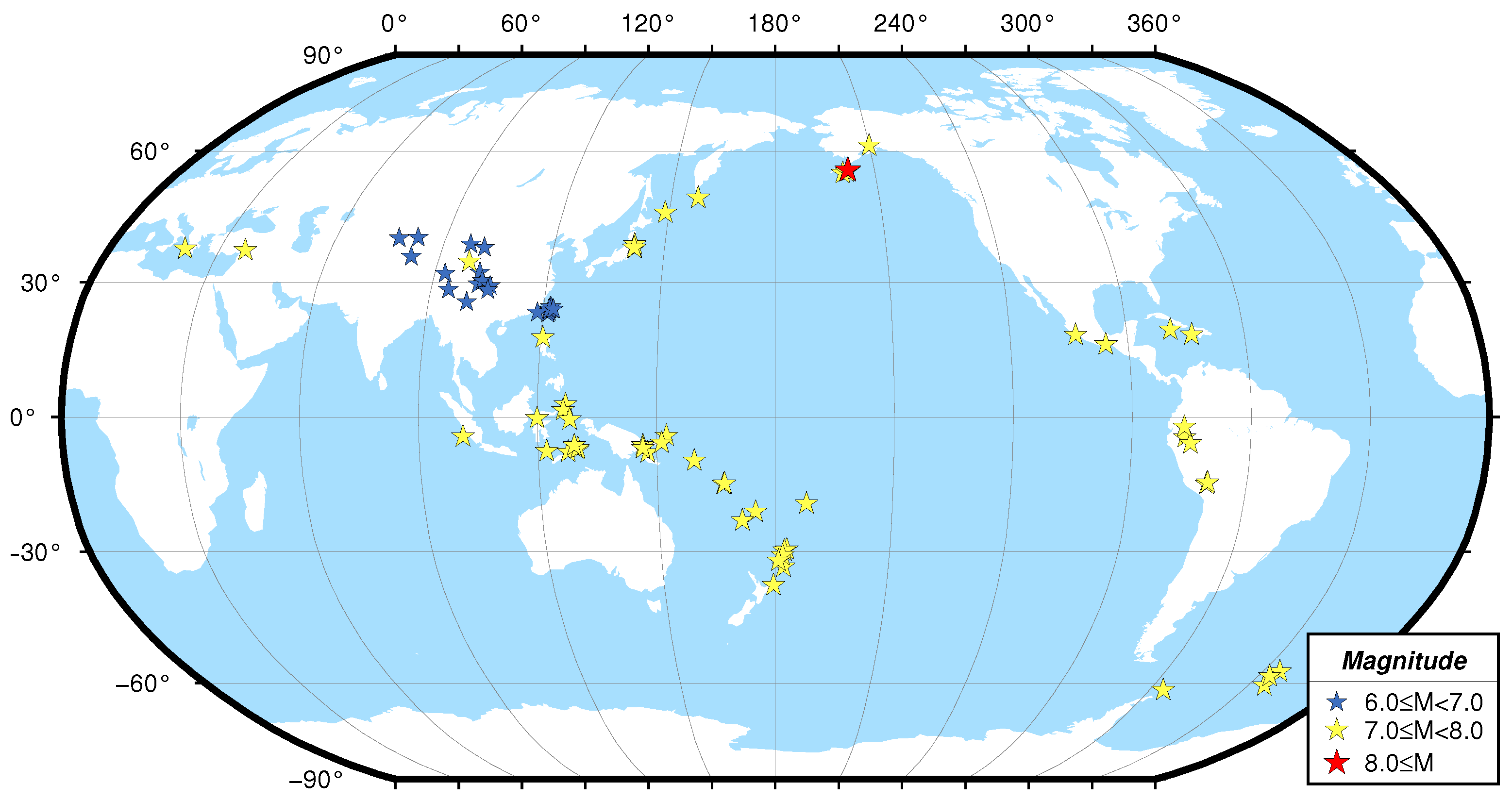
- We ensured that seismic events were not located within the South Atlantic Anomaly (SAA) region or the outer radiation belts.
- The time window considered spanned 15 days before the EQ to 5 days after the EQ. This time is a conclusion accumulated from previous research.
- We determined that the anomaly falls within the Dobrovolsky radius, which is approximately ±10 in latitude and longitude from the EQ epicenter.
- Anomalous fluxes were more than 0.5 orders of magnitude above the “no-anomalous” period in the same region, and this condition was rated as highly significant. We can identify anomalies in the high–energy particle flux figures easily with visual interpretation.
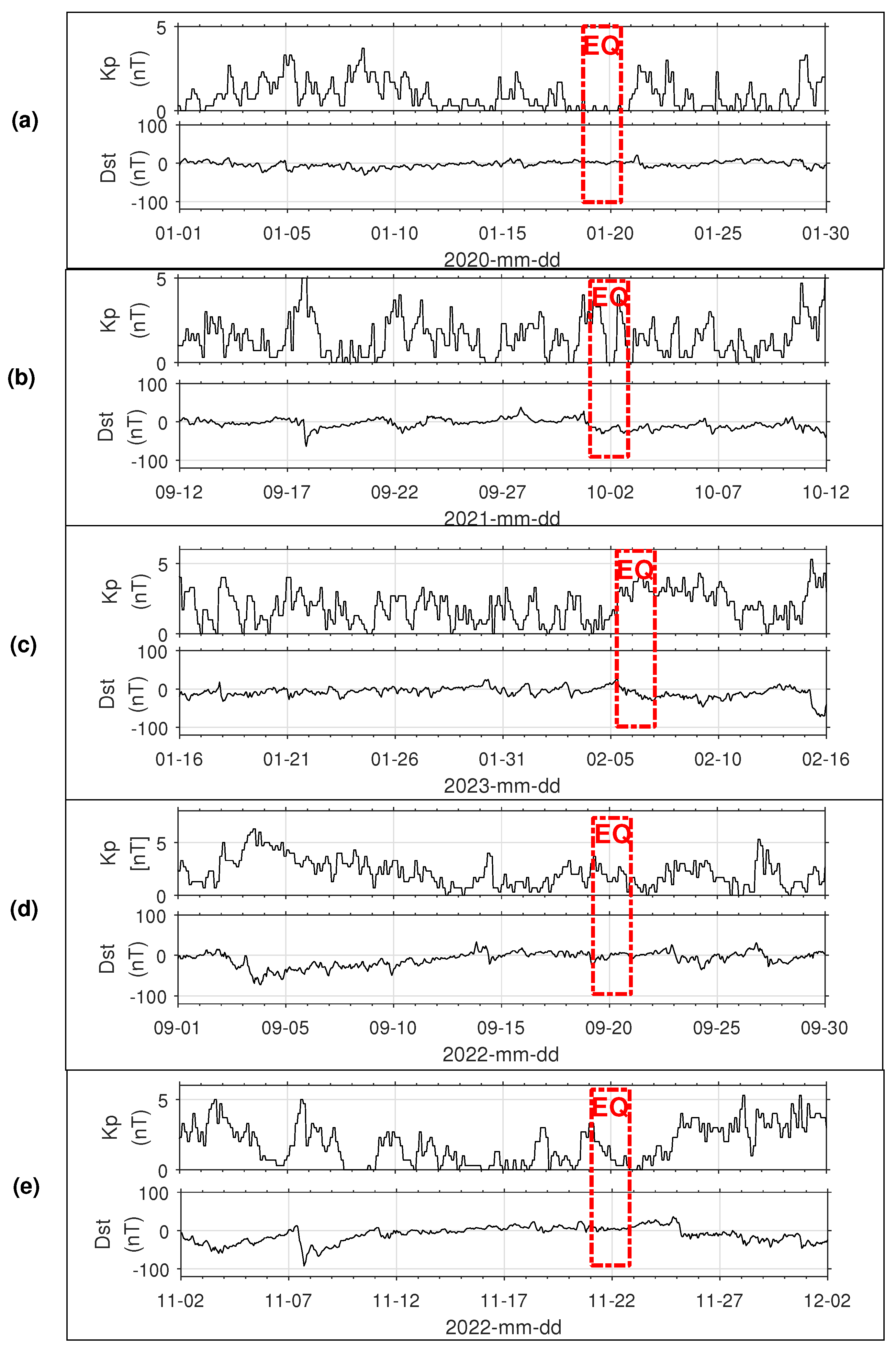
- We compared the Dst index and determined if the anomaly was caused by a space weather event (Dst ≤−30 nT).
3. Results
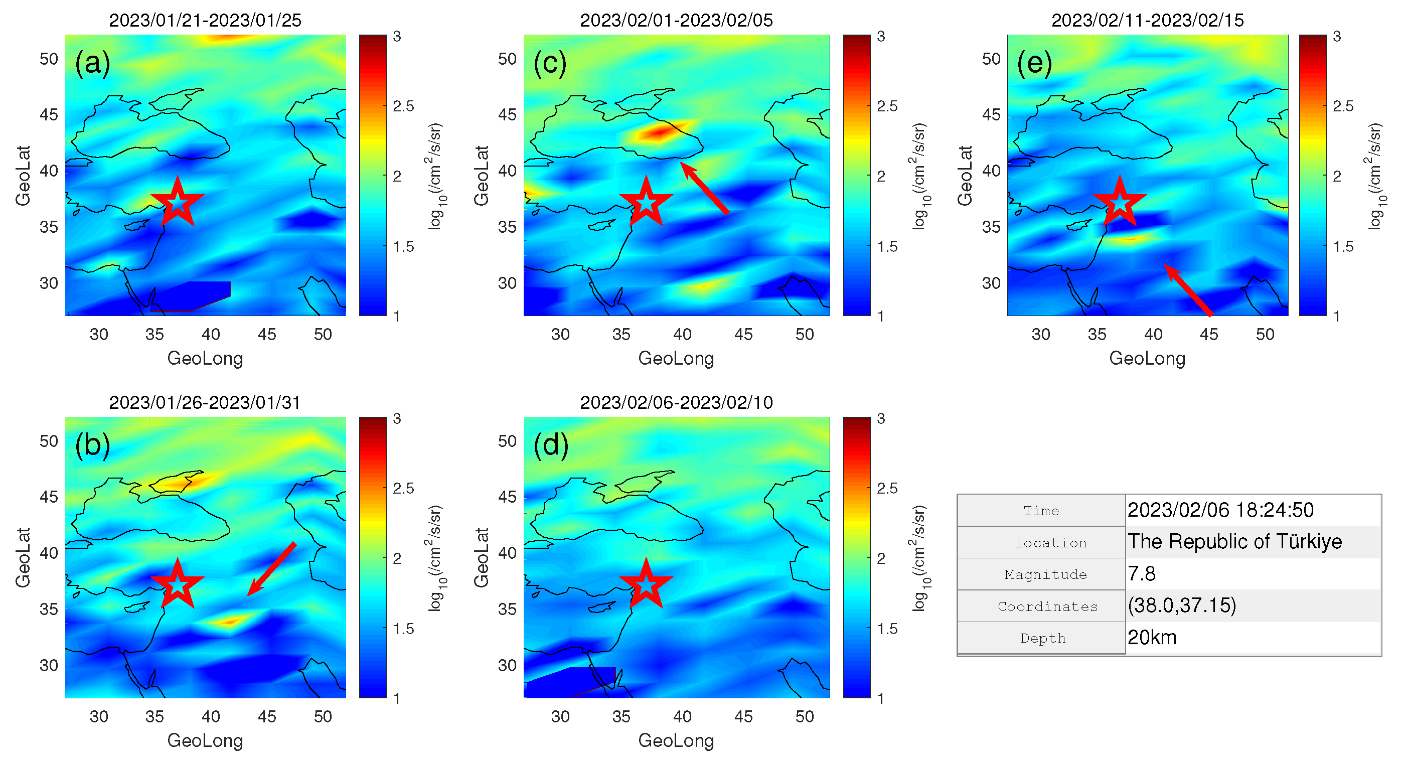
3.1. Electron Spatial Distribution Evolution Related to EQs
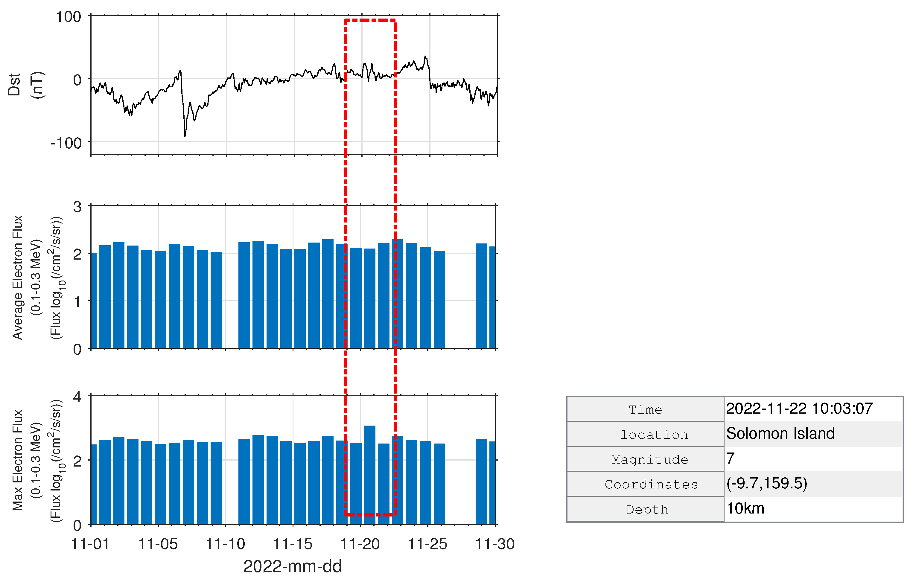
3.2. Time Evolution of Electrons Flux Related with EQs
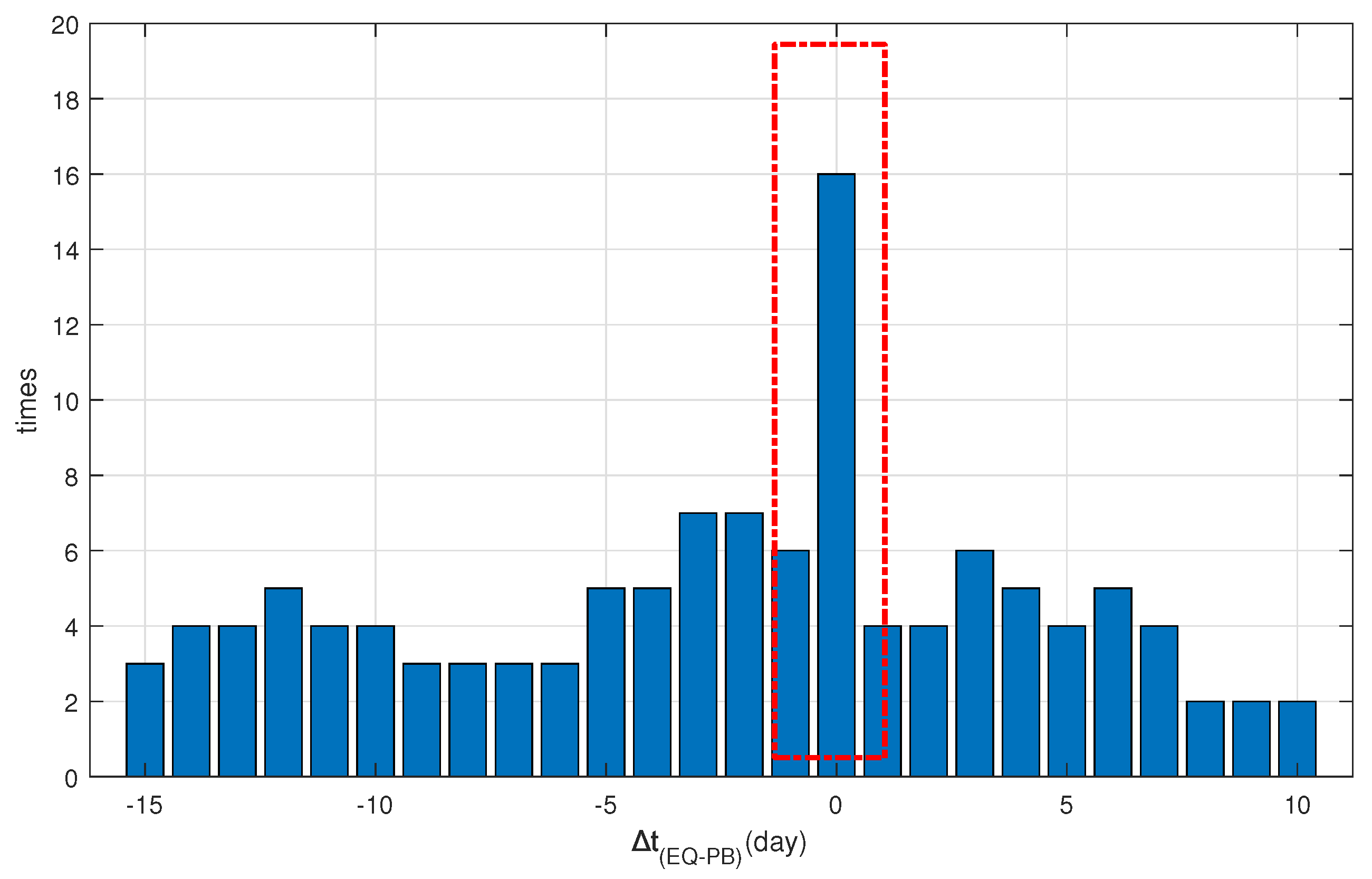
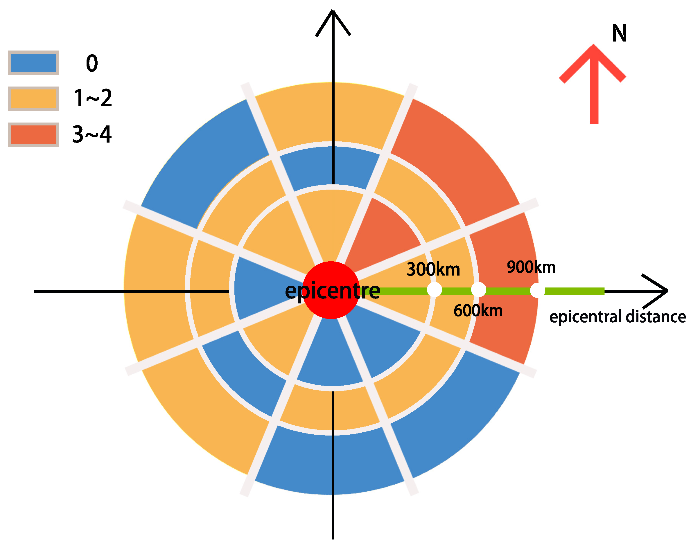
3.3. Statistical Results of High–Energy Particle Disturbance Characteristics before Strong EQs
3.4. Possible Mechanism: Wave–Particle Interactions in Earthquakes
4. Conclusions and Discussion
- Among the 78 EQ cases, we excluded 16 cases from the statistical work. In the remaining 62 cases, 39 cases showed electron flux anomalies, which included spatial distribution or temporal distribution, and possibly both. Overall, the probability of EQ–related electron flux anomalies was 62%.
- From the time distribution, the highest probability of anomalies was found on the current day of the EQ, with a total of 16 in 78 EQ cases. In addition, there were many anomalies that occurred during the 5 days before the EQ.
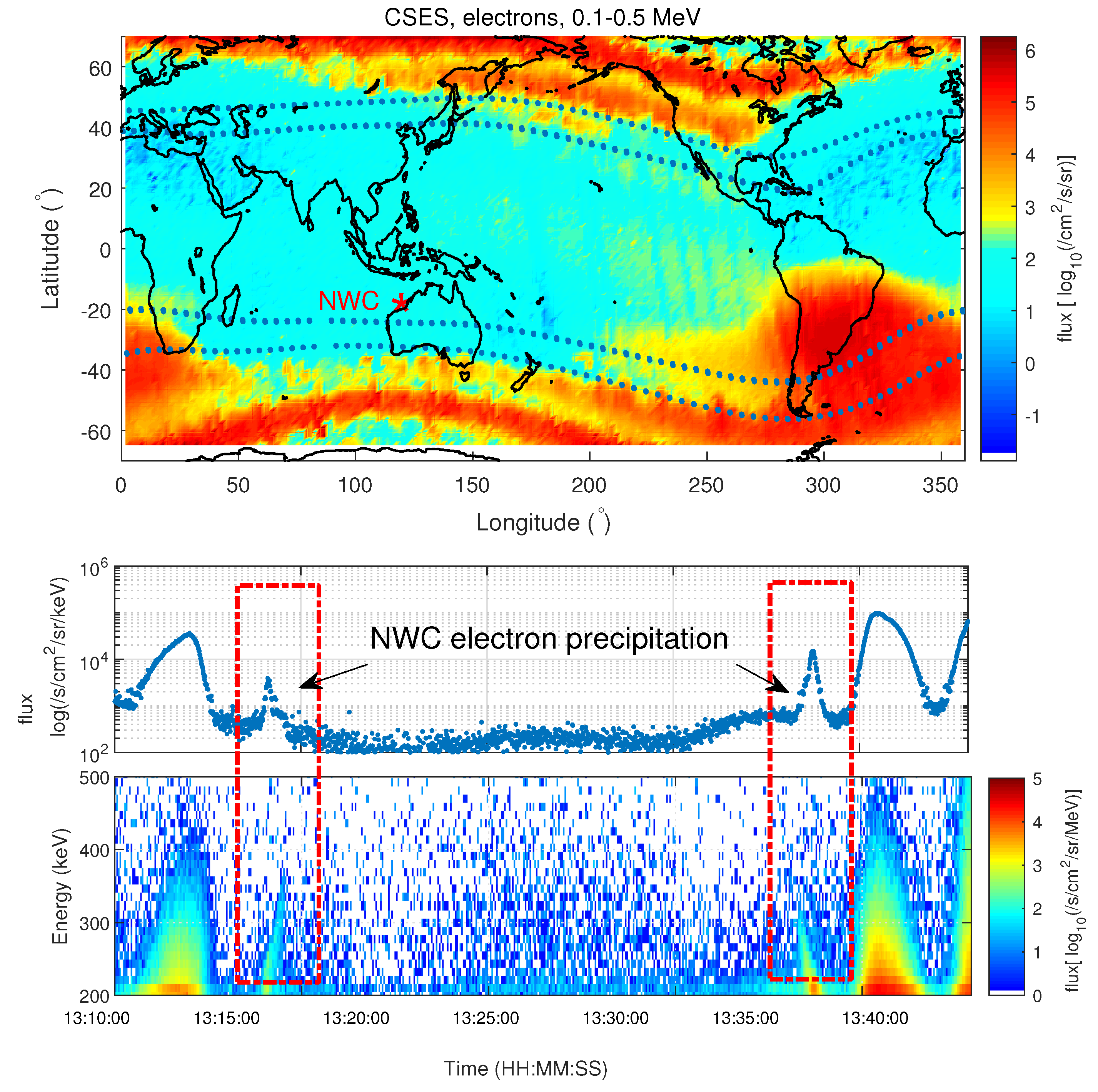
- We also investigated the spatial distribution of the perturbation. The northeast was the most likely direction to show anomalies, followed by the east. This phenomenon was consistent with the distribution of electron precipitation belt caused by the ground stations NWC, which is a wisp.
- In terms of distance, the largest probability of anomalous electron precipitation occurred within the range of about 600–900 km from the epicenter, with 11 times, which is a percentage of .
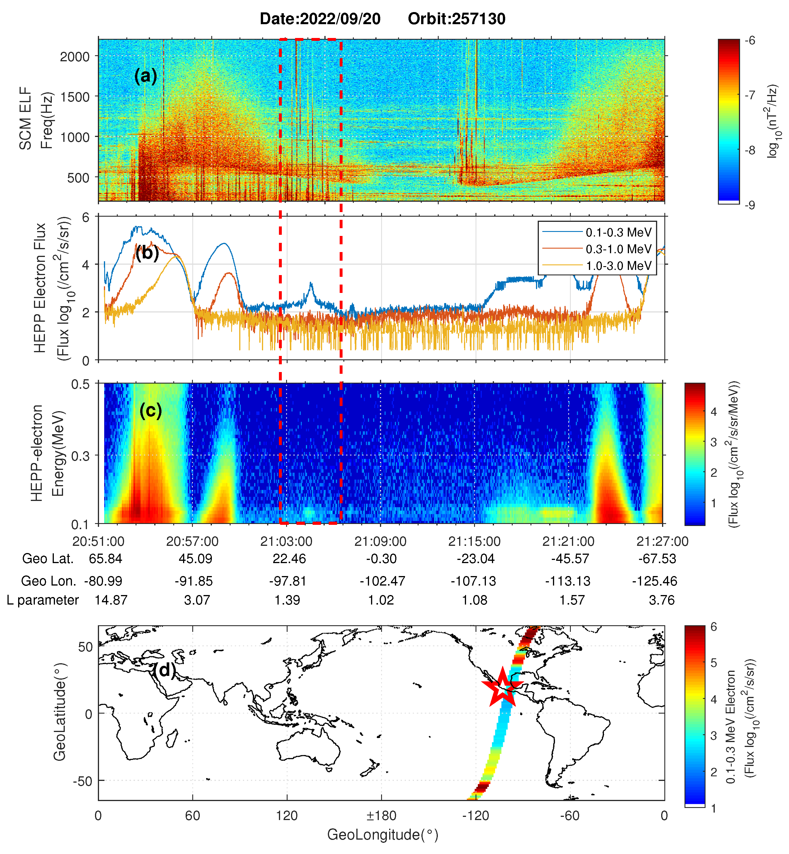
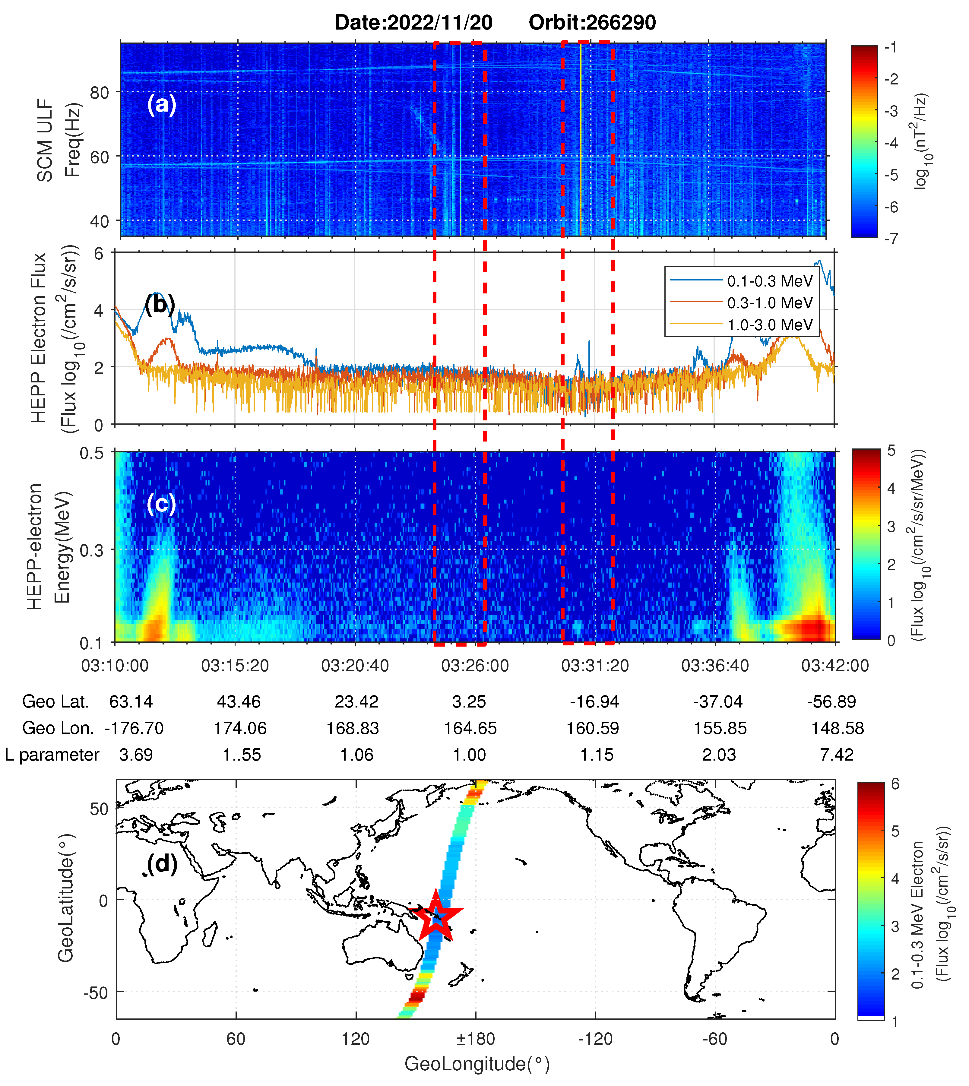
- The anomalous precipitation of the high–energy particle flux during the EQ may be accompanied with electromagnetic wave perturbations and wave–particle interactions. We also presented two earthquake cases accompanied by anomalous electromagnetic waves. Electromagnetic waves excited by earthquakes interact with electrons in the radiation belt in a wave–particle interaction, which may be a probable explanation for the generation of electron precipitation during EQs. More research will be carried out for this part in the future.
Author Contributions
Funding
Data Availability Statement
Acknowledgments
Conflicts of Interest
References
- Pulinets, S.; Boyarchuk, K. Ionospheric Precursors of Earthquakes; Springer: Berlin/Heidelberg, Germany, 2004; pp. 142–149. [Google Scholar]
- Aleksandrin, S.Y.; Galper, A.M.; Grishantzeva, L.A.; Koldashov, S.V.; Maslennikov, L.V.; Murashov, A.M.; Picozza, P.; Sgrigna, V.; Voronov, S.A. High–energy charged particle bursts in the near-Earth space as earthquake precursors. Ann. Geophys. 2003, 21, 597–602. [Google Scholar] [CrossRef]
- Heki, K. Ionospheric electron enhancement preceding the 2011 Tohoku–Oki earthquake. Geophys. Res. Lett. 2011, 38, 456. [Google Scholar] [CrossRef]
- Zhang, X.; Fidani, C.; Huang, J.; Shen, X.; Zeren, Z.; Qian, J. Burst increases of precipitating electrons recorded by the DEMETER satellite before strong earthquakes. Nat. Hazards Earth Syst. Sci. 2013, 13, 197–209. [Google Scholar] [CrossRef]
- Voronov, S.A.; Galper, A.M.; Koldashov, S.V. Observation of high energy charged particle flux increases in SAA region in 10 September 1985. Cosm. Res. 1989, 27, 629–631. [Google Scholar]
- Ruzhin, Y.Y.; Depueva, A.K. Seismo Precursors in Space as Plasma and Wave Anomalies. J. Atmos. Electr. 1996, 16, 271–288. [Google Scholar]
- Sgrigna, V.; Carota, L.; Conti, L.; Corsi, M.; Galper, A.M.; Koldashov, S.V.; Murashov, A.M.; Picozza, P.; Scrimaglio, R.; Stagni, L. Correlations between earthquakes and anomalous particle bursts from SAMPEX/PET satellite observations. J. Atmos. Sol.-Terr. Phys. 2005, 67, 1448–1462. [Google Scholar] [CrossRef]
- Parrot, M.; Berthelier, J.J.; Lebreton, J.P.; Sauvaud, J.A.; Santolík, O.; Blecki, J. Examples of unusual ionospheric observations made by the DEMETER satellite over seismic regions. Phys. Chem. Earth 2006, 31, 486–495. [Google Scholar] [CrossRef]
- Zhang, Z.X.; Wang, C.Y.; Shen, X.H.; Li, X.Q.; Wu, S.G. Study of typical space wave–particle coupling events possibly related with seismic activity. Chin. Phys. B 2014, 23, 109401. [Google Scholar] [CrossRef]
- Li, X.; Ma, Y.; Wang, P.; Wang, H.; Lu, H.; Zhang, X.; Huang, J.; Shi, F.; Yu, X.; Xu, Y.; et al. Study of the North West Cape electron belts observed by DEMETER satellite. J. Geophys.-Res.-Space Phys. 2012, 117, A04201. [Google Scholar] [CrossRef]
- Yan, R.; Wang, L.W.; Zhang, S.Z. The electromagnetic disturbance study based on the observational data form satellite and ground station during a magnetic storm. Adv. Mater. Res. 2013, 804, 180–186. [Google Scholar] [CrossRef]
- Fidani, C. Improving earthquake forecasting by correlations between strong earthquakes and NOAA electron bursts. Terr. Atmos. Ocean. Sci. 2018, 29, 1–14. [Google Scholar] [CrossRef]
- Fidani, C.; Battiston, R. Analysis of NOAA particle data and correlations to seismic activity. Nat. Hazards Earth Syst. 2008, 8, 1277–1291. [Google Scholar] [CrossRef]
- Roberto, B.; Vincenzo, V. First evidence for correlations between electron fluxes measured by NOAA-POES satellites and large seismic events. Nucl. Phys. B-Proc. Suppl. 2013, 249–257, 243–244. [Google Scholar]
- Pulinets, S.A.; Boyarchuk, K.A.; Hegai, V.V.; Kim, V.P.; Lomonsov, A.M. Quasielectrostatic model of atmosphere–thermosphere– ionosphere coupling. Adv. Space Res. 2000, 26, 1209–1218. [Google Scholar] [CrossRef]
- Sorokin, V.M.; Chmyrev, V.M.; Yaschenko, A.K. Electrodynamic model of the lower atmosphere and the ionosphere coupling. Atmos. Sol.-Terr. Phys. 2001, 63, 1681–1691. [Google Scholar] [CrossRef]
- Sorokin, V.M.; Yaschenko, A.K.; Hayakawa, M.A. Perturbation of DC electric fifield caused by light ion adhesion to aerosols during the growth in seismic-related atmospheric radioactivity. Nat. Hazards Earth Syst. 2007, 7, 155–163. [Google Scholar] [CrossRef]
- Zhao, S.; Zhang, X.M.; Zhao, Z.; Shen, X. The numerical simulation on ionospheric perturbations in electric field before large earthquakes. Ann. Geophys. 2014, 32, 1487–1493. [Google Scholar] [CrossRef]
- Anagnostopoulos, G.C.; Vassiliadis, E.; Pulinets, S. Characteristics of flux-time profiles, temporal evolution, and spatial distribution of radiation-belt electron precipitation bursts in the upper ionosphere before great and giant earthquakes. Ann. Geophys. 2012, 55, 1. [Google Scholar] [CrossRef]
- Chakraborty, S.; Sasmal, S.; Basak, T.; Chakrabarti, S.K. Comparative study of charged particle precipitation from Van Allen radiation belts as observed by NOAA satellites during a land earthquake and an ocean Earthquake. Adv. Space Res. 2019, 64, 719–732. [Google Scholar] [CrossRef]
- Summers, D.; Ma, C.A. A model for generating relativistic electrons in the Earth’s inner magnetosphere based on gyroresonant wave-particle interactions. J. Geophys. Res. 2020, 105, 2625–2639. [Google Scholar] [CrossRef]
- Frolov, V.L.; Akchurin, A.D.; Bolotin, I.A.; Ryabov, A.O.; Berthelier, J.J.; Parrot, M. Precipitation of Energetic Electrons from the Earth Radiation Belt Stimulated by High-Power HF Radio Waves for Modification of the Midlatitude Ionosphere. Radiophys. Quantum Electron. 2020, 62, 571–590. [Google Scholar] [CrossRef]
- Zhang, Z.X.; Li, X.Q.; Chen, L.J. North west cape-induced electron precipitation and theoretical simulation. Chin. Phys. B 2016, 25, 119401. [Google Scholar] [CrossRef]
- Parrot, M. Statistical study of ELF/VLF emissions recorded by a low-altitude satellite during seismic events. J. Geophys. Res. 1994, 99, 23339–23347. [Google Scholar] [CrossRef]
- Parrot, M. VLF emissions associated with earthquakes and observed in the ionosphere and the magnetosphere. Earth Planet. Inter. 1989, 57, 86–99. [Google Scholar] [CrossRef]
- Wang, Q.; Huang, J.; Zhao, S.; Zhima, Z.; Yan, R.; Lin, J.; Yang, Y.; Chu, W.; Zhang, Z.; Lu, H.; et al. The electromagnetic anomalies recorded by CSES during Yangbi and Madoi earthquakes occurred in late May 2021 in west China. Nat. Hazards Res. 2022, 1, 10. [Google Scholar] [CrossRef]
- Yan, R.; Zhima, Z.; Xiong, C.; Shen, X.; Huang, J.; Guan, Y.; Zhu, X.; Liu, C. Comparison of Electron Density and Temperature from the CSES Satellite With Other Space-Borne and Ground-Based Observations. J. Geophys. Res. Space Phys. 2020, 125, e2019JA027747. [Google Scholar] [CrossRef]
- Yan, R.; Xiong, C.; Zhima, Z.; Shen, X.; Liu, D.; Liu, C.; Guan, Y.; Zhu, K.; Zheng, L.; Lv, F. Correlation Between Ne and Te Around 14:00 LT in the Topside Ionosphere Observed by CSES, Swarm and CHAMP Satellites. Front. Earth Sci. 2022, 10, 860234. [Google Scholar] [CrossRef]
- Zhima, Z.; Hu, Y.; Shen, X.; Chu, W.; Piersanti, M.; Parmentier, A.; Zhang, Z.; Wang, Q.; Huang, J.; Zhao, S.; et al. Storm-Time Features of the Ionospheric ELF/VLF Waves and Energetic Electron Fluxes Revealed by the China Seismo-Electromagnetic Satellite. Appl. Sci. 2021, 11, 2617. [Google Scholar] [CrossRef]
- Zhima, Z.; Hu, Y.; Pierstanti, M.; Shen, X.; De Santis, A.; Yan, R.; Yang, Y.; Zhao, S.; Zhang, Z.; Wang, Q. The seismic electromagnetic emissions during the 2010 Mw 7.8 Northern Sumatra Earthquake revealed by DEMETER satellite. Front. Earth Sci. 2020, 8, 459. [Google Scholar] [CrossRef]
- Zhima, Z.; Yan, R.; Lin, J.; Wang, Q.; Yang, Y.; Lv, F.; Huang, J.; Cui, J.; Liu, Q.; Zhao, S.; et al. The Possible Seismo-Ionospheric Perturbations Recorded by the China-Seismo-Electromagnetic Satellite. Remote Sens. 2022, 14, 905. [Google Scholar] [CrossRef]
- Zhu, K.; Zheng, L.; Yan, R.; Shen, X.; Zeren, Z.; Xu, S.; Chu, W.; Liu, D.; Zhou, N.; Guo, F. Statistical study on the variations of electron density and temperature related to seismic activities observed by CSES. Nat. Hazards Res. 2021, 1, 88–94. [Google Scholar] [CrossRef]
- Shen, X.H.; Zhang, X.M.; Yuan, S.G.; Wang, L.W.; Cao, J.B.; Huang, J.P. The state-of-the-art of the China Seismo-Electromagnetic Satellite mission. Sci. China Technol. Sci. 2018, 61, 634–642. [Google Scholar] [CrossRef]
- Li, X.Q.; Xu, Y.B.; An, Z.H.; Liang, X.H.; Wang, P.; Zhao, X.Y.; Wang, H.Y.; Lu, H.; Ma, Y.Q.; Shen, X.H.; et al. The high–energy particle package onboard CSES. Radiat. Detect. Technol. Methods 2019, 3, 22. [Google Scholar] [CrossRef]
- Zhang, Z.; Li, X.; Wang, L.; Zhima, Z.; Shen, X.; Yuan, S.; An, Z.; Xu, Y.; Liang, X.; Zhang, D.; et al. Evaluation of the proton contamination to MeV electrons by solar proton events based on CSES observations. Ournal Geophys. Res. Space Phys. 2022, 127, e2022JA030550. [Google Scholar] [CrossRef]
- Cao, J.; Zeng, L.; Zhan, F.; Wang, Z.; Wang, Y.; Chen, Y.; Meng, Q.; Ji, Z.; Wang, P.; Liu, Z. The electromagnetic wave experiment for CSES mission: Search coil magnetometer. Sci. China Technol. 2018, 61, 653–658. [Google Scholar] [CrossRef]
- Dobrovosky, I.R.; Zubkov, S.I.; Myachkin, V.I. Estimation of the size of earthquake preparation zones. Pageoph 1979, 117, 1025–1044. [Google Scholar] [CrossRef]


| No. | Time | M. | Lat. | Long. | Place | Space Weather | Perturbation |
|---|---|---|---|---|---|---|---|
| 1 | 23 February 2023 | 7.2 | 37.98 | 73.29 | Tajikistan | A moderate geomagnetic storm occurred two days before the EQ | Slightly elevated electron flux the day before the EQ |
| 2 | 26 May 2022 | 7.2 | −14.85 | −70.3 | Peruvian | Quiet | Near the SAA region |
| 3 | 28 November 2021 | 7.3 | −4.5 | −76.7 | Northern Peru | Quiet | Near the SAA region |
| 4 | 23 August 2021 | 7 | −60.55 | −24.9 | South Sandwich Islands | Quiet | Near the SAA region |
| 5 | 14 August 2021 | 7 | 55.3 | −157.75 | Alaska, USA | Quiet | Near the outer radiation belt |
| 6 | 13 August 2021 | 7.6 | −57.21 | −24.81 | South Sandwich Islands | Quiet | Near the SAA region, near the outer radiation belt |
| 7 | 29 July 2021 | 8.1 | 55.4 | −158 | Alaska, USA | Quiet | Near the outer radiation belt |
| 8 | 24 January 2021 | 7 | −61.7 | −55.6 | South Shetland Islands | Quiet | Near the SAA region |
| 9 | 20 October 2020 | 7.5 | 54.74 | −159.75 | Alaska, USA | Quiet | Near the outer radiation belt |
| 10 | 19 August 2020 | 7 | −4.31 | 101.15 | Sumatra, Indonesia | A moderate geomagnetic storm occurred on the day of the EQ | Slightly elevated electron flux one day after the EQ, ruled out by magnetic storms |
| 11 | 22 July 2020 | 7.8 | 55.05 | −158.5 | Alaska, USA | Quiet | Near the outer radiation belt |
| 12 | 16 June 2020 | 7.2 | −30.8 | −178.1 | New Zealand Kermadec Islands | Quiet | Near the outer radiation belt |
| 13 | 26 May 2019 | 7.8 | −5.85 | −75.18 | Northern Peru | Quiet | Near the SAA region |
| 14 | 1 March 2019 | 7 | −14.58 | −70.05 | Peruvian | Quiet | Near the SAA region |
| 15 | 11 December 2019 | 7 | −58.35 | −26.37 | South Sandwich Islands | Quiet | Near the outer radiation belt |
| 16 | 1 December 2019 | 7.2 | 61.35 | −150.06 | Alaska, USA | Quiet | Near the outer radiation belt |
| No. | Time | M. | Lat. | Long. | Place | Perturbation |
|---|---|---|---|---|---|---|
| 1 | 6 February 2023 | 7.8 | 37.15 | 36.95 | Turkey | Ten days before the EQ, an anomaly occurred 500 km southeast of the epicenter. Five days before the EQ, an anomaly occurred 800 km northeast of the epicenter. Five days after the EQ, an anomaly appeared 300 km south of the epicenter. |
| 2 | 30 January 2023 | 6.1 | 40.01 | 82.29 | Aksu, Xinjiang | No apparent abnormality. |
| 3 | 18 January 2023 | 7 | 2.8 | 127.1 | Indonesia | Two days before the EQ, there was an anomaly in the daily maximum electron flux in the range of 0.3–3.0 MeV, night side. |
| 4 | 10 January 2023 | 7.6 | −7.2 | 130.1 | Indonesia | No apparent abnormality. |
| 5 | 8 January 2023 | 7 | −14.95 | 166.8 | Vanuatu | Fifteen days before the EQ, there was an anomaly in the daily maximum electron flux in the range of 0.1–0.3 MeV, night side. |
| 6 | 22 November 2022 | 7 | −9.7 | 159.5 | Solomon Island | Fifteen days before the EQ, there was a slight rise in the night–side 0.1–0.3 MeV electron flux about 1000 km east of the epicenter. |
| 7 | 11 November 2022 | 7.4 | −19.25 | −172.05 | Tonga Islands | Ten days before the EQ, an anomaly occurred 500 km in east of the epicenter. |
| 8 | 20 September 2022 | 7.5 | 18.3 | −103.2 | Mexico | Twelve days before the EQ, there was an anomaly in the daily maximum electron flux in the range of 0.3–3.0 MeV, day side. |
| 9 | 18 September 2022 | 6.9 | 23.15 | 121.3 | Hualien, Taiwan | On the day of the EQ, there was an anomaly in the daily maximum electron flux in the range of 0.3–3.0 MeV, day side. |
| 10 | 11 September 2022 | 7.6 | −6.3 | 146.55 | Papua New Guinea | Five days after the EQ, an anomaly occurred directly above the epicenter. |
| 11 | 5 September 2022 | 6.8 | 29.59 | 102.08 | Luding, Sichuan | On the day of the EQ, there was an anomaly in the daily maximum electron flux in the range of 0.3–3.0 MeV, day side. |
| 12 | 27 July 2022 | 7 | 17.7 | 120.55 | Philippine | No apparent abnormality. |
| 13 | 10 June 2022 | 6 | 32.25 | 101.82 | Malcolm, Sichuan | On the day of the EQ, there was an anomaly in the daily maximum electron flux in the range of 0.3–3.0 MeV, day side. |
| 14 | 1 June 2022 | 6.1 | 30.37 | 102.94 | Ya’an, Sichuan | No apparent abnormality. |
| 15 | 9 May 2022 | 6.2 | 24.01 | 122.51 | Hualien, Taiwan | No apparent abnormality. |
| 16 | 26 March 2022 | 6 | 38.5 | 97.33 | Haixi, Qinghai | On the day of the EQ, there was an anomaly in the daily maximum electron flux in the range of 0.3–3.0 MeV, night side. |
| 17 | 23 March 2022 | 6.6 | 23.45 | 121.55 | Taitung, Taiwan | No apparent abnormality. |
| 18 | 16 March 2022 | 7.4 | 37.65 | 141.95 | Japan | No apparent abnormality. |
| 19 | 8 January 2022 | 6.9 | 37.77 | 101.26 | Haibei, Qinghai | No apparent abnormality. |
| 20 | 3 January 2022 | 6.4 | 24 | 122.39 | Hualien, Taiwan | On the day of the EQ, there was an anomaly in the daily maximum and average electron flux in the range of 0.3–3.0 MeV, night side. |
| 21 | 30 December 2021 | 7.5 | −7.75 | 127.6 | Banda Sea | On the day of the EQ, there was an anomaly in the daily maximum and average electron flux in the range of 0.3–3.0 MeV, night side. Five days after the EQ, an anomaly occurred directly above the epicenter and 500 km west of the epicenter. |
| 22 | 14 December 2021 | 7.3 | −7.6 | 122.2 | Flores Sea | In the 2–3 days of the EQ, there was an anomaly in the daily maximum electron flux in the range of 0.3–3.0 MeV, day side. |
| 23 | 24 October 2021 | 6.3 | 24.55 | 121.8 | Yilan, Taiwan | Five days after the EQ, an anomaly occurred 300 km northeast of the epicenter. |
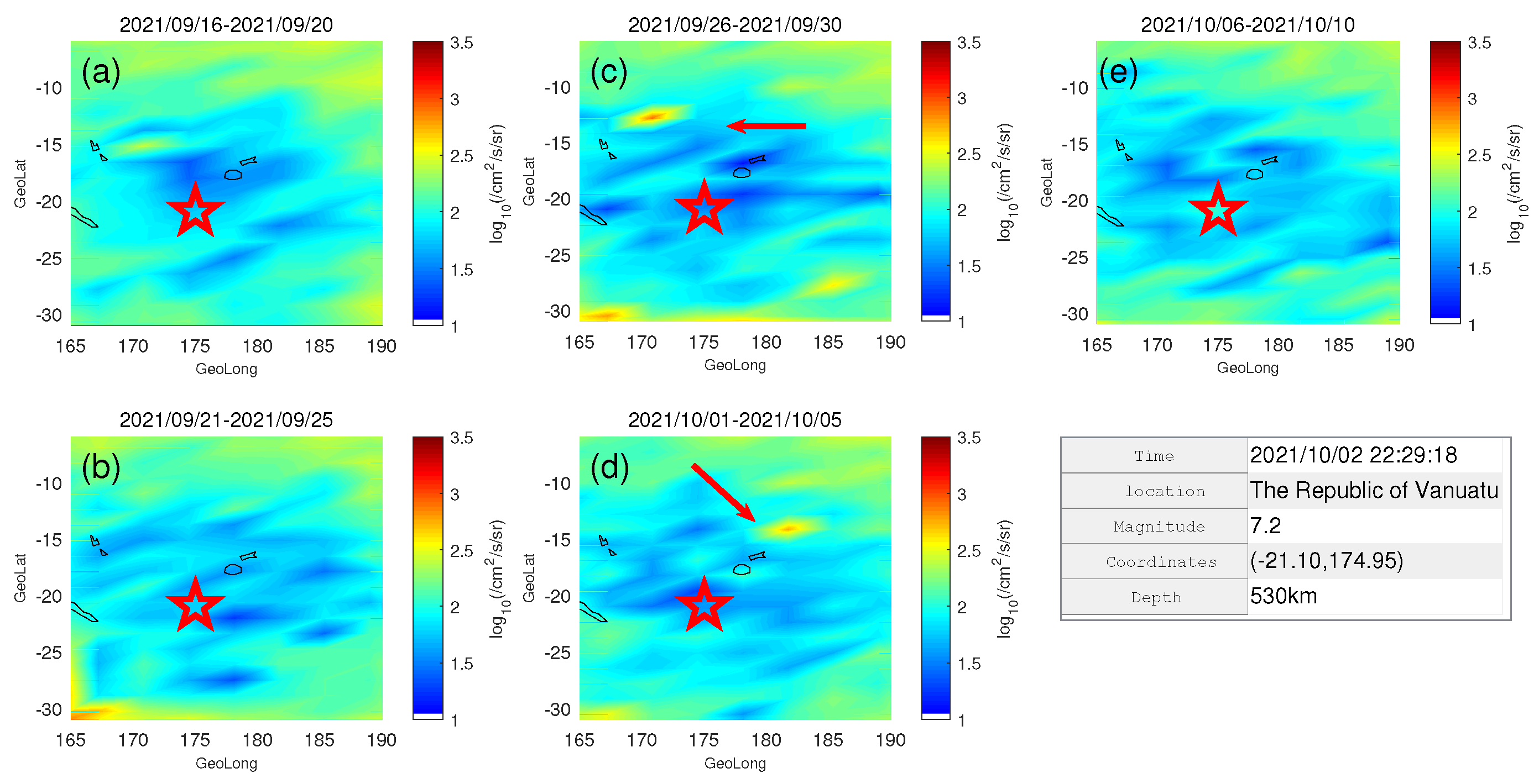
| 24 | 2 October 2021 | 7.2 | −21.1 | 174.95 | Vanuatu | In the 5 days of the EQ, an anomaly occurred 600 km northeast of the epicenter. Five days after the EQ, an anomaly occurred 800 km northeast of the epicenter. |
| 25 | 16 September 2021 | 6 | 29.2 | 105.34 | Luzhou, Sichuan | No apparent abnormality. |
| 26 | 8 September 2021 | 7.1 | 17.12 | −99.6 | Mexico | Five days before the EQ, an anomaly occurred 800 km east of the epicenter. |
| 27 | 18 August 2021 | 7 | −14.79 | 167.04 | Vanuatu | Five days after the EQ, an anomaly occurred 300 km east of the epicenter. For 2–3 days of the EQ, there was an anomaly in the daily maximum electron flux in the range of 0.3–3.0 MeV, night side. |
| 28 | 14 August 2021 | 7.3 | 18.35 | −73.45 | Haiti | On the day of the EQ, there was an anomaly in the daily maximum electron flux in the range of 0.3–3.0 MeV, night side. |
| 29 | 22 May 2021 | 7.4 | 34.59 | 98.34 | Mado, Qinghai | On the day of the EQ, there was an anomaly in the daily maximum electron flux in the range of 0.3–3.0 MeV, day side. |
| 30 | 21 May 2021 | 6.4 | 25.67 | 99.87 | Dali, Yunnan | On the day of the EQ, there was an anomaly in the daily maximum electron flux in the range of 0.3–3.0 MeV, night side. |
| 31 | 18 April 2021 | 6.1 | 23.94 | 121.43 | Hualien, Taiwan | On the day of the EQ, there was an anomaly in the daily maximum electron flux in the range of 0.3–3.0 MeV, dayside. |
| 32 | 20 March 2021 | 7 | 38.43 | 141.84 | Japan | On the day of the EQ, there was an anomaly in the daily maximum electron flux in the range of 0.3–3.0 MeV, night side. |
| 33 | 19 March 2021 | 6.1 | 31.94 | 92.74 | Nagchu, Tibet | The 5 days of the EQ, an anomaly occurred 500 km northeast of the epicenter. |
| 34 | 5 March 2021 | 7.8 | −29.51 | −177.04 | New Zealand Kermadec Islands | Ten days before the EQ, an anomaly occurred 300 km southeast of the epicenter. |
| 35 | 13 February 2021 | 7.1 | 37.7 | 141.8 | Japan | Ten days before the EQ, an anomaly occurred 100 km north of the epicenter. |
| 36 | 10 February 2021 | 7.4 | −23.05 | 171.5 | Loyalty Islands | Ten days before the EQ, an anomaly occurred 300 km northeast of the epicenter. |
| 37 | 17 July 2020 | 7 | −7.86 | 147.7 | Papua New Guinea | Fifteen days before the EQ, an anomaly occurred 300 km south of the epicenter. One day and three days before the EQ, there was an anomaly in the daily maximum electron flux in the range of 0.3–3.0 MeV, night side. |
| 38 | 26 June 2020 | 6.4 | 35.73 | 82.33 | Hotan, Xinjiang | The 5 days of the EQ, an anomaly occurred 1000 km northeast of the epicenter. |
| 39 | 23 June 2020 | 7.4 | 16.14 | −95.75 | Mexico | No apparent abnormality. |
| 40 | 18 June 2020 | 7.3 | −33.35 | −177.85 | New Zealand Kermadec Islands | No apparent abnormality. |
| 41 | 6 May 2020 | 7.2 | −6.93 | 130.07 | Indonesia | On the day of the EQ, there was an anomaly in the daily maximum electron flux in the range of 0.3–3.0 MeV, day side. |
| 42 | 25 March 2020 | 7.5 | 48.93 | 157.74 | Kuril island chain | No apparent abnormality. |
| 43 | 13 February 2020 | 7 | 45.6 | 148.95 | Kuril island chain | No apparent abnormality. |
| 44 | 29 January 2020 | 7.7 | 19.46 | −78.79 | Southern Cuban waters | No apparent abnormality. |
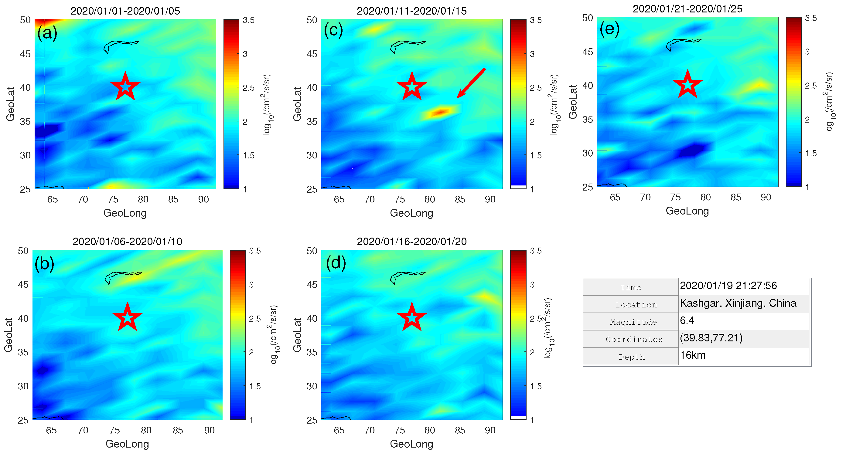
| 45 | 19 January 2020 | 6.4 | 39.83 | 77.21 | Qeshqer, Xinjiang | Two days before the EQ, there was an anomaly in the daily maximum electron flux in the range of 0.3–3.0 MeV, day side. Five days before the EQ, an anomaly occurred 500 km southeast of the epicenter. |
| 46 | 15 November 2019 | 7.2 | 1.55 | 126.48 | Indonesia | On the day of the EQ, there was an anomaly in the daily maximum electron flux in the range of 0.3–3.0 MeV, day side. |
| 47 | 8 August 2019 | 6.4 | 24.52 | 121.96 | Yilan, Taiwan | Five days before the EQ, an anomaly occurred 400 km southnortheast of the epicenter. |
| 48 | 14 July 2019 | 7.1 | −0.52 | 128.17 | Indonesia | No apparent abnormality. |
| 49 | 24 June 2019 | 7.3 | −6.36 | 129.24 | Haiti | No apparent abnormality. |
| 50 | 17 June 2019 | 6 | 28.34 | 104.9 | Yibin, Sichuan | No apparent abnormality. |
| 51 | 14 May 2019 | 7.6 | −4.15 | 152.52 | New Britain region | Three days before the EQ, there was an anomaly in the daily maximum electron flux in the range of 0.3–3.0 MeV, day side. Ten days before the EQ, an anomaly occurred 500 km west of the epicenter. |
| 52 | 7 May 20197 | 7.1 | −6.96 | 146.49 | Papua New Guinea | No apparent abnormality. |
| 53 | 24 April 2019 | 6.3 | 28.4 | 94.61 | Linzhi, Tibet | On the day of the EQ, there was an anomaly in the daily maximum electron flux in the range of 0.3–3.0 MeV, night side. |
| 54 | 18 April 2019 | 6.7 | 24.02 | 121.65 | Hualien, Taiwan | Three days after the EQ, there was an anomaly in the daily maximum electron flux in the range of 0.3–3.0 MeV, night side. |
| 55 | 22 February 2019 | 7.5 | −2.15 | −76.91 | Ecuador | No apparent abnormality. |
| 56 | 26 November 2018 | 6.2 | 23.28 | 118.6 | Taiwan Strait | The 5 days of the EQ, an anomaly occurred 1000 km east of the epicenter. |
| 57 | 26 October 2018 | 7 | 37.51 | 20.51 | Ionian Sea | No apparent abnormality. |
| 58 | 23 October 2018 | 6 | 24.01 | 122.65 | Hualien, Taiwan | The 5 days of the EQ, an anomaly occurred 800 km east of the epicenter. |
| 59 | 11 October 2018 | 7.1 | −5.7 | 151.25 | Papua New Guinea | Ten days before the EQ, an anomaly occurred 10,300 km southwest of the epicenter. |
| 60 | 28 September 2018 | 7.4 | −0.25 | 119.9 | Indonesia | No apparent abnormality. |
| 61 | 10 September 2018 | 7 | −31.95 | −179.25 | Kermadec Islands | No apparent abnormality. |
| 62 | 6 September 2018 | 7.8 | −18.45 | 179.35 | Fiji | No apparent abnormality. |
Disclaimer/Publisher’s Note: The statements, opinions and data contained in all publications are solely those of the individual author(s) and contributor(s) and not of MDPI and/or the editor(s). MDPI and/or the editor(s) disclaim responsibility for any injury to people or property resulting from any ideas, methods, instructions or products referred to in the content. |
© 2023 by the authors. Licensee MDPI, Basel, Switzerland. This article is an open access article distributed under the terms and conditions of the Creative Commons Attribution (CC BY) license (https://creativecommons.org/licenses/by/4.0/).
Share and Cite
Wang, L.; Zhang, Z.; Zhima, Z.; Shen, X.; Chu, W.; Yan, R.; Guo, F.; Zhou, N.; Chen, H.; Wei, D. Statistical Analysis of High–Energy Particle Perturbations in the Radiation Belts Related to Strong Earthquakes Based on the CSES Observations. Remote Sens. 2023, 15, 5030. https://doi.org/10.3390/rs15205030
Wang L, Zhang Z, Zhima Z, Shen X, Chu W, Yan R, Guo F, Zhou N, Chen H, Wei D. Statistical Analysis of High–Energy Particle Perturbations in the Radiation Belts Related to Strong Earthquakes Based on the CSES Observations. Remote Sensing. 2023; 15(20):5030. https://doi.org/10.3390/rs15205030
Chicago/Turabian StyleWang, Lu, Zhenxia Zhang, Zeren Zhima, Xuhui Shen, Wei Chu, Rui Yan, Feng Guo, Na Zhou, Huaran Chen, and Daihui Wei. 2023. "Statistical Analysis of High–Energy Particle Perturbations in the Radiation Belts Related to Strong Earthquakes Based on the CSES Observations" Remote Sensing 15, no. 20: 5030. https://doi.org/10.3390/rs15205030