

Geo-Environment Vulnerability Assessment of Multiple Geohazards Using VWT-AHP: A Case Study of the Pearl River Delta, China
School of Environmental Studies, China University of Geosciences, Wuhan 430000, China
*
Author to whom correspondence should be addressed.
Remote Sens. 2023, 15(20), 5007; https://doi.org/10.3390/rs15205007
Submission received: 15 September 2023
/
Revised: 15 October 2023
/
Accepted: 16 October 2023
/
Published: 18 October 2023
(This article belongs to the Topic Natural Hazards and Disaster Risks Reduction)
Abstract
:Geohazards pose significant risks to communities and infrastructure, emphasizing the need for accurate susceptibility assessments to guide land-use planning and hazard management. This study presents a comprehensive method that combines Variable Weight Theory (VWT) with Analytic Hierarchy Process (AHP) to assess geo-environment vulnerability based on susceptibility to various geohazards. The method was applied to the Pearl River Delta in China, resulting in the classification of areas into high vulnerability (5961.85 km2), medium vulnerability (19,227.93 km2), low vulnerability (14,892.02 km2), and stable areas (1616.19 km2). The findings demonstrate improved accuracy and reliability compared to using AHP alone. ROC curve analysis confirms the enhanced performance of the integrated method, highlighting its effectiveness in discerning susceptibility levels and making informed decisions in hazard preparedness and risk reduction. Additionally, this study assessed the risks posed by geohazards to critical infrastructures, roads, and artificial surfaces, while discussing prevention strategies. However, this study acknowledges certain limitations, including the subjective determination of its judgment matrix and data constraints. Future research could explore the integration of alternative methods to enhance the objectivity of factor weighting. In practical applications, this study contributes to the understanding of geo-environment vulnerability assessments, providing insight into the intricate interplay among geological processes, human activities, and disaster resilience.
1. Introduction
Geohazards encompass a range of geological processes occurring on the Earth’s surface influenced by interactions among the atmosphere, hydrosphere, and biosphere [1]. Geohazards, notably landslides and debris flows, have caused significant human casualties and property losses, reaching billions of dollars [2,3]. Improving geohazard risk management is a crucial global effort aimed at mitigating the consequences of geohazards [4]. Geo-environment vulnerability assessment is an effective tool for enhancing disaster management. It can assess susceptibility to various geohazards, offering proactive strategies for disaster reduction. Consequently, it can contribute significantly to promoting symbiosis and sustainable development between humanity and the natural environment.
Vulnerability stands as a metric extensively harnessed in the fields of climate change, resource environments, and ecosystems [5,6,7,8,9,10,11]. Due to variations in research subjects and disciplinary perspectives, the definition of vulnerability can vary significantly among disciplines [12]. Initially introduced by Margat (1968) [13] in a study on groundwater pollution susceptibility, vulnerability is defined as the ability of groundwater to resist contamination based on hydrogeological conditions. Timmerman (1981) [14] defined vulnerability from the perspective of climate change as the degree to which a system responds unfavorably when subjected to damage. Smit et al. (1999) [15], at the scale of global change, described vulnerability as the extent to which a system is susceptible to harm or injury. Research in the field of geo-environment vulnerability remains limited, leading to a lack of a universal definition for geo-environment vulnerability. In this study, geo-environment vulnerability is considered the capacity of a geo-environmental system to autonomously regulate and reinstate its structure and functionality amid external disruptions [16]. The magnitude of geo-environment vulnerability depends on the components and configuration of the system, intertwined with the nature and intensity of external perturbations. When the intensity of external disturbances surpasses the system’s self-regulatory capacities, latent geo-environment vulnerability transforms into geo-environmental issues or geohazards [17]. Consequently, the susceptibility status of geohazards can characterize geo-environment vulnerability [17]. The impact and duration of geohazards vary, occurring in isolation or conjunction. Thus, conducting vulnerability assessments based on a range of geohazards is essential, rather than relying on the susceptibility to a single type of geohazard [18,19].
Advancements in remote sensing (RS) technology and geographic information systems (GIS) have contributed to the maturity of geo-environment vulnerability assessment techniques. Ma et al. (2019) [17] assessed the geo-environment vulnerability of Beihai, China, based on the susceptibility to landslides, collapses, and sea water intrusion. Ma et al. (2020) [20] assessed the geo-environmental risk in Zhengzhou, China, considering regional crustal stability and 11 types of geohazards and progressive geo-environmental issues. Chang et al. (2022) [21] researched the susceptibility of landslides, collapses, ground subsidence, and debris flows, proposing a multi-hazard vulnerability assessment method. Li et al. (2023) [22] developed an assessment framework for the ecological geo-environment vulnerability of arid and semi-arid cities, focusing on land desertification, soil erosion, and landslides. While these studies have made progress, there is currently no unified quantitative scoring standard, and research on geo-environment vulnerability assessment in large urban clusters is limited [23]. These limitations hinder the ability to balance socio-economic development and effective decision-making for geohazard prevention and control.
Multiple methods exist for assessing susceptibility to geohazards, classified into the following four primary categories: process-based modeling methods, statistical methods, machine learning methods, and knowledge-driven methods [24]. Process-based modeling methods simulate the occurrence processes of geohazards, grounded in physical or mathematical principles and capable of delivering precise susceptibility predictions [25]. However, their applicability to regional-scale studies is limited due to the substantial requirements of detailed field data and extensive computational simulations [26]. Statistical methods, such as Frequency Ratio (FR) [27], Logistic Regression (LR) [28], and Weight of Evidence (WoE) [29], rely on extensive data and statistical analysis, with result accuracy closely associated with statistical assumptions [26]. Machine learning methods, such as Support Vector Machine (SVM) [30], Random Forest (RF) [31], and Artificial Neural Network (ANN) [32], manage multidimensional data and complex linear relationships but may face challenges related to interpretability and data quality [26,33]. Knowledge-driven methods are flexible approaches relying on the judgment of decision-makers or experts based on their knowledge and experience, offering high decision-making efficiency and effectiveness [34]. These methods are adaptable to various spatial and temporal scales and suitable for a wide range of applications. They are particularly valuable when data is limited or unavailable, allowing for assessments even in data-scarce scenarios [35].
Multi-Criteria Decision Analysis (MCDA) is a fundamental knowledge-driven method, recognized as an essential tool for environmental decision-making, enabling the visualization and resolution of competitive decision problems [36,37,38,39]. By integrating qualitative and quantitative criteria, MCDA has become a cornerstone in integrated problem-solving solutions [40]. Among the suite of MCDA techniques, the Analytic Hierarchy Process (AHP) emerges as a fitting choice for grappling with intricate issues [41]. AHP is a framework that ascertains the relative significance of factors through pairwise comparisons and expert assessments, harmonizing subjective and objective criteria [42,43]. This method deconstructs complex problems into distinct factors, systematically arranging them in a hierarchical manner according to their interrelationships, yielding a multi-level analytical structural model [44].
While AHP furnishes unchanging factor weights across varying conditions, the values of these factors exhibit diversity amidst different circumstances. Consequently, AHP falls short in capturing the dynamic fluctuations of factor weights within distinct contexts [45]. The core concept of the Variable Weight Theory (VWT) involves introducing a state-variable weight vector while retaining the stability of factor weights. This theoretical framework comprises three distinctive modes: penalization-based, incentive-based, and a hybrid form combining both penalization and incentive elements [46]. This method guarantees the flexibility of weight adjustments in alignment with varying factor values and specific contextual circumstances, thereby presenting an effective resolution to these complexities [47].
China is significantly impacted by global geohazards, evident from the mounting intensity and frequency of such incidents [48]. In recent times, driven by rapid socio-economic growth and urbanization, the Pearl River Delta, as one of the largest urban clusters in China, has experienced an expansion in geological environmental development and utilization. Characterized by intricate tectonics, extensive karst landscapes, and widespread Quaternary deposits, the area faces natural catastrophes including landslides, collapses, and debris flows, resulting in substantial economic losses [49,50,51,52]. Data from the Guangdong Province Disaster Prevention and Reduction Yearbook [53] show that between 1994 and 2009, geohazards caused 276 fatalities, 534 injuries, and economic losses totaling 256.48 million US dollars. Research on the geo-environment vulnerability in the Pearl River Delta primarily focuses on two aspects: geological environmental status assessments and single geohazard susceptibility assessments. Zeng and Liu (2015) [54] conducted an investigation into key geo-environmental issues in the Pearl River Delta, including ground subsidence, sea water intrusion, and waste pollution. The study identified rising sea levels, human activities, and extreme weather events as the primary triggering factors for geohazards. In a separate study, Zhang et al. (2019) [55] employed the AHP method to assess landslide susceptibility. Dou et al. (2008) [56] introduced an innovative automated detection method for karst collapse based on image analysis. Liu et al. (2023) [57] conducted ground subsidence modeling and assessment using remote sensing imagery and geological data. Furthermore, Lin et al. (2019) [58] employed an integrated Bayesian model for modeling sea water intrusion. Presently, there exists a notable dearth of comprehensive assessments regarding geological environmental vulnerability. Given the presence of geohazards, such as landslides, debris flows, ground subsidence, and karst collapses, the assessment of geo-environment vulnerability based on susceptibility to multiple geohazards is crucial for effective prevention and mitigation, ensuring human safety and protecting valuable assets.
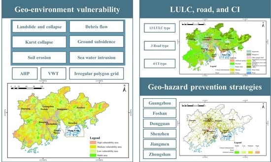
Using the AHP method, this study partitioned geo-environment vulnerability into discrete dimensions: landslide and collapse susceptibility, debris flow susceptibility, karst collapse susceptibility, ground subsidence susceptibility, soil erosion susceptibility, and sea water intrusion susceptibility. Comprehensive assessment indicators and classification criteria were delineated for each dimension. Judgment matrices were formulated to establish constant weights of individual indicators. Moreover, a “penalization-incentive” variant of the VWT was adeptly utilized to dynamically adjust the weights of these indicators. By assessing the susceptibility to distinct geohazards, the methodology subsequently defined distinct zones of geo-environment vulnerability. Based on the assessment results and in conjunction with the distribution of land use/land cover (LULC), road, and critical infrastructure, the impact of geohazard susceptibility and geo-environment vulnerability on urban development was discussed. The specific research objectives are as follows:
- 1.
- Propose a multi-hazard geological disaster susceptibility assessment system using the VWT-AHP method.
- 2.
- Analyze the geo-environment vulnerability in the Pearl River Delta.
- 3.
- Provide recommendations for LULC, road, and critical infrastructure planning.
The implications of the findings from this assessment hold substantial pertinence for local governing bodies, providing invaluable insights for the formulation of land use planning and strategies for industrial development.
2. Study Area
Situated in the central-southern expanse of Guangdong Province, China, the Pearl River Delta shares its borders with the South China Sea. Geographically, it spans longitudinally from approximately 112°0′E to 115°24′E and latitudinally from 21°43′N to 23°56′N, encompassing a land area of 41,698 km2. The region’s topography features a central lowland and elevations that ascend in the northwest and east (Figure 1b). A dominant landform is the alluvial plain, with low mountains, hills, and tablelands distributed across the western, northern, and eastern sectors (Figure 1a). The region’s hydrology is extensive, characterized by river systems such as the Xi River and Dong River, which emanate from mountainous terrains and discharge into the South China Sea. The climatic conditions prevailing in this study area are warm and humid, with an average annual temperature of 21.9 °C. Monsoonal influences lead to pronounced temporal and spatial variations in precipitation, with a concentrated peak during the summer months. The yearly average precipitation amounts to approximately 1600 mm, with certain mountainous locales experiencing levels ranging from 2000 mm to 2600 mm (Figure 1c).
The study area exhibits a comprehensive and diverse development of geological strata, with extensive distribution patterns. Encompassing a broad spectrum, geological formations range from the ancient, highly metamorphosed rocks of the Mesoproterozoic era to the more recent loose clastic sediments of the Quaternary period. Geological dynamics in this region are primarily characterized by significant, episodic fluctuations in elevation and subsidence, accompanied by differential block movements. The demarcation of boundaries is predominantly dictated by fault lines, while the internal structure is further influenced by the intersection of secondary faults oriented in various directions. Drawing from the attributes, origins, and structural traits of lithological entities, the geological compositions in the study area are classified into six primary categories: unconsolidated soil, intrusive rocks, volcanic rocks, metamorphic rocks, clastic rocks and carbonate rocks (Figure 2). Groundwater predominantly exists within the interstices of loose sediments, fractures within carbonate rocks, and fissures in bedrock.
3. Methods and Materials
3.1. Technical Route
In this study, the assessment of landslide and collapse susceptibility, debris flow susceptibility, karst collapse susceptibility, ground subsidence susceptibility, soil erosion susceptibility, and sea water intrusion susceptibility was carried out utilizing the VWT-AHP method. Furthermore, the assessment of geo-environment vulnerability was conducted by drawing parallels with the principle of the “barrel effect”. Based on the assessment results and considering the distribution of LULC, road construction, and critical infrastructure, recommendations for geohazard prevention and mitigation were provided. The flowchart for this study is depicted in Figure 3.
3.2. Database
3.2.1. Geo-Hazard Inventory
The geological environmental challenges in the study area are predominantly characterized by occurrences of collapses, landslides, debris flows, karst collapses, ground subsidence, and soil erosion, showcasing a widespread distribution (Figure 4). As of 2020, there are 83 locations with landslides and collapses posing a threat to over 100 people, 23 locations with debris flows endangering more than 100 people, and 97 locations experiencing karst collapses. Ground subsidence exceeding 10 cm has been documented in 65 locations. Soil erosion takes the form of a fragmented distribution within the research zone, covering 1.76% of the total study area. Employing a criterion of Total Dissolved Solids (TDS) exceeding 1 g/L, the Pearl River Estuary region experiences a discernible degree of seawater intrusion, affecting approximately 10.87% of the total area. The distribution map of geohazards was provided by the Guangdong Geological Survey Institute.
3.2.2. Assessment Indicators
In this study, a total of 34 factors were selected for assessing the susceptibility to six types of geohazards. Details regarding the data types, resolutions, temporal coverages, and sources of these factors are detailed in Table 1.
Landslide and collapse susceptibility. Landslides refer to the downward movement of rock and soil masses along weak surfaces under the influence of gravity, whereas collapses involve the abrupt detachment of soil or rock masses from their parent materials, resulting in vertical descent and potential rolling and accumulation along slopes. Numerous factors trigger landslides and collapses, including heavy precipitation, lithology, seismic activity, geomorphic processes, and human activities [61,62]. These events predominantly occur in mountainous and valley regions, characterized by steep topography and significant elevation differences. Steeper slopes with intense terrain incision are more prone to landslides and collapses due to concentrated stress at steeper angles. Geological factors such as lithology and geological structures play pivotal roles in landslides and collapses. Lithology serves as the fundamental condition determining the possibility of these events, while geological structures influence the development of fractures within rocks. In regions marked by fault zones and the presence of weak rocks, fissures within rocks lead to structural looseness, reduced shear strength, and diminished resistance to weathering. Greater fissure development and rock fragmentation heighten the likelihood of landslides and collapses. Precipitation is a critical triggering factor, as water infiltrates through rock fractures, eroding and softening the material, promoting further fissure expansion, weakening the mechanical strength of rocks, and simultaneously eroding slope angles, thus forming precipitous faces. In this study, the selected assessment indicators encompassed elevation, slope, lithology, topography, distance to fault, distance to river, and precipitation [63,64,65,66,67]. Slope data was computed using ArcGIS 10.6 based on the elevation data. River data was extracted from remote sensing images and the distance to river was calculated using ArcGIS 10.6 with the Euclidean distance method.
Debris flow susceptibility. Debris flow entails the rapid surging of a mixture comprising water, sediment, rocks, and soil on steep slopes, often triggered by heavy precipitation. They exhibit high speeds, extended propagation distances, and significant destructive potential [68,69,70]. In regions characterized by intense fissure development, active faulting, and abundant landslides, fragmented rocks constitute the material basis for debris flow occurrence. Precipitation plays a pivotal role as a triggering factor for mudflows, as intense precipitation generates temporary surface runoff that provides the dynamic conditions for mudflow initiation. Debris flows predominantly occur in steep mountainous terrain, where unstable slopes are prone to landslides and collapses, facilitating the rapid accumulation of fragmented rock masses. Debris flows frequently follow river valleys and ravines, which facilitate the convergence of water flow and the transportation of eroded rock–soil material. For this study, the chosen assessment indicators encompassed elevation, slope, lithology, topography, distance to fault, distance to river, distance to landslide and collapse, and precipitation [71,72,73,74]. The distance to landslide and collapse was calculated using ArcGIS 10.6 with the Euclidean distance method.
Karst collapse susceptibility. Karst collapse refers to the abrupt sinking and deformation of loose rock–soil material overlaying soluble rock layers with well-developed karst cavities, resulting from the collapse of the terrain. The presence of karst caves is a prerequisite for karst collapse occurrences. The concentration of stress induced by surrounding rock dynamics on the roofs and sidewalls of karst caves impairs their stability. The extent of karst formation, the quantity, and dimensions of karst caves all contribute to heightened susceptibility to karst collapses. Groundwater inflow augments the weight of the cave roof rock mass, coursing through fractures to diminish shear resistance between adjacent rock segments and exacerbate the erosion of soluble rock, thereby intensifying karst development. Greater fragmentation of the soluble rock mass corresponds to more advanced fissuring, rendering it increasingly susceptible to groundwater erosion. This study incorporated a range of assessment indicators for karst collapse susceptibility, including lithology, degree of karst development, thickness of overlying layer, water yield property, and distance to fault [31,75,76,77].
Ground subsidence susceptibility. Ground subsidence refers to the abrupt or gradual downward movement of the Earth’s surface, primarily in the vertical dimension, with minimal lateral shifts [78]. Ground subsidence is frequently instigated by excessive groundwater extraction [79]. A fundamental prerequisite for ground subsidence is the presence of an overlaying stratum of soft soil. The drainage of water from the soft soil results in diminished pore water pressure and amplification of effective stress, leading to the consolidation and densification of the soft soil layer. Crustal movements can also trigger ground subsidence, typically manifesting at a comparably sluggish pace. In this study, the chosen assessment indicators encompassed thickness of soft soil layer, age of soft soil layer, water yield property, and distance to fault [80,81,82,83].
Soil erosion susceptibility. Soil erosion is the phenomenon in which soil particles disperse, transport, and submerge under the influence of hydraulic processes and human activities. Climate, topography, land cover, and land use conditions are pivotal factors shaping soil erosion dynamics [84,85]. The physical structure of soil serves as the substrate for soil erosion, with loosely compacted soil structures and reduced viscosity rendering it more susceptible to erosion caused by water and human actions. Precipitation-induced surface runoff acts as a fundamental driving force behind soil erosion, with higher precipitation intensities leading to increased runoff volumes and escalated erosion potential. Slope gradient stands as a critical determinant in soil erosion resistance, as steeper slopes elevate the propensity of soil mass movement due to gravitational forces, thereby intensifying surface runoff and augmenting erosion risks. Vegetation plays a crucial role in intercepting precipitation, thus mitigating surface runoff intensity. Root systems contribute to water retention and soil compaction, thereby ameliorating the impact of soil erosion. In this study, the selected assessment indicators for soil erosion susceptibility encompassed slope, topography, type of vegetation, type of soil, distance to river, and precipitation [86,87,88].
Sea water intrusion susceptibility. Sea water intrusion pertains to the process whereby freshwater aquifers undergo salinization due to both natural and human-induced factors [89]. The manifestation of sea water intrusion necessitates the fulfillment of two conditions: the existence of hydraulic conduits and a disparity in hydraulic pressure within the aquifer. In coastal aquifers characterized by porous or fractured substrates, as well as those shaped by karst formations, sea water gains access to the groundwater system through these pathways. As the hydraulic head of sea water surpasses that of the coastal aquifer, driven by this hydraulic gradient, sea water infiltrates the groundwater reservoir via hydraulic connections. The replenishment of groundwater, which potentially leads to an increase in groundwater levels within coastal aquifers, can occur through mechanisms like precipitation-induced infiltration. In this study, the chosen indicators for assessing sea water intrusion susceptibility encompassed topography, type of Quaternary sedimentary rock, groundwater level, and precipitation [90,91,92,93].
Each indicator has been assigned ratings of 0.1, 0.3, 0.7, and 0.9 across four ranges. In cases where an indicator is categorized into three ranges, its ratings were adjusted to 0.1, 0.3, and 0.7. The delineation of factor ranges and assignment of ratings are derived from previous studies [94,95,96,97,98]. The ranges and ratings of all indicators are presented in Table 2. The distribution maps of all indicators are available in Figure 5, Figure 6, Figure 7, Figure 8, Figure 9 and Figure 10.
3.2.3. LULC, Road, and Critical Infrastructure
In the study area, there are 13 LULC types (Figure 11). Artificial surfaces are predominantly found in urban areas, particularly in Guangzhou and Shenzhen. The area also includes both paddy fields and dryland and economic crops mainly include banana, citrus, and sugarcane. The mountainous areas exhibit significant variation in vegetation cover, ranging from less than 30% to over 90%. The LULC data for the year 2020 was provided by the Guangdong Geological Survey Institute.
The road network encompasses national highways, provincial roads, and railways, while critical infrastructure comprises facilities related to education, energy, healthcare, and water resources. All data was sourced from OSM (2023) [99].
3.3. Methods
3.3.1. Analytic Hierarchy Process
The AHP, introduced by Saaty (1980) [42], is known for its simplicity in principle and dependable theoretical foundation. Abundant practical cases have demonstrated the significant applicability of AHP in effectively addressing complex multi-objective competitive decision-making problems [100,101,102,103,104]. The AHP generally involves the following three steps:
- Step 1: Develop a multi-level hierarchical structure model.
The multi-level hierarchical structure elucidates the interplays among various constituents within complex challenges [105]. Factors are categorized into distinct strata based on their attributes, with each stratum subordinate to higher-level factors and capable of influencing lower-level factors. The identification of factors primarily relies on existing knowledge and expertise.
- Step 2: Conduct pairwise comparisons of factors and formulate judgment matrices.
Based on the assessments of decision-makers or experts, the relative importance of factors is determined through pairwise comparisons. For these comparisons, a scale from 1 to 9 is used (Table 3). The judgment matrix A, derived from these pairwise comparisons, is used to calculate the weights of each factor. Matrix A is represented in Equation (1). The dimension n of the matrix corresponds to the number of factors.
To reduce significant variations among the elements within the judgment matrix A, a normalization procedure is applied to the matrix elements. The calculation method for normalizing the elements within the matrix is outlined in Equation (2).
To calculate the eigenvector corresponding to the maximum eigenvalue, the average of the row elements of the normalized matrix is calculated as described in Equation (3).
The method for calculating the maximum eigenvalue is outlined in Equation (4).
- Step 3: Determine factor weights and perform consistency checks.
The coherence of pairwise comparisons plays a pivotal role in influencing the precision of decisions made by evaluators. Improved coherence corresponds to more accurate outcomes in these pairwise assessments. When coherence is found to be lacking, a re-examination of the pairwise comparisons among factors becomes imperative. The procedure for computing the Consistency Index (CI), an indicator used to quantify the consistency of the judgment matrix, is explained in Equation (5).
To calculate the Consistency Ratio (CR), the first step involves establishing the Average Random Consistency Index (RI), as guided by the values provided in Table 4.
The equation to calculate the CR, used for addressing inconsistencies, is provided by Equation (6). A CR value less than or equal to 0.10 is considered acceptable for maintaining a reasonable level of consistency.
3.3.2. Variable Weight Theory
In the context of the AHP, the conventional assumption assumes the constancy of factor weights. However, in practical scenarios, factors with exceptionally high or low values can significantly impact assessment outcomes. To address this issue, this study introduces the VWT, a mechanism that dynamically adjusts the weights of factors based on their values. This adaptation enhances the fidelity of assessment results in representing complex real-world contexts.
The VWT, initially introduced by Wang (1985) [106], has garnered significant attention and application across diverse fields [107,108,109,110]. This theory presents a framework that establishes a linkage between weight vectors and state vectors, enabling the adaptation of factor weights by shifts in decision states.
To better reflect the impact of extreme values on indicator weights, this study introduces a “penalization-incentive” variant of the VWT. The definitions of the state variable weight vector and the variable weight vector are provided, along with their corresponding calculation methods presented in Equations (7) and (8), respectively.
In Equations (7) and (8), the symbol xj represents the rating of the i-th indicator, si signifies the state variable weight vector corresponding to the i-th indicator, wi denotes the constant weight vector associated with the i-th indicator, and wi’ indicates the variable weight vector of the i-th indicator. The parameters are subject to the conditions 0 < λ < α < β < μ < 1 and 0 < c < b < a < 1. In this study, the parameter values were set as follows: λ = 0.2, α = 0.4, β = 0.6, μ = 0.8, c = 0.2, b = 0.3, and a = 0.5 [111].
Finally, the Comprehensive Index (CPI) is determined by Equation (9).
3.3.3. Assessment Unit Segmentation
The irregular polygon grid method was used to segment assessment units [112]. Specifically, for each geohazard, the distribution maps of all indicators were superimposed using ArcGIS 10.6 to generate a susceptibility distribution map. Each closed polygon with uniform ratings was treated as an individual assessment unit, thus eliminating rating inconsistencies within the same unit that could introduce errors. The irregular polygons formed by overlaying the susceptibility distribution maps were considered as the assessment units for geo-environment vulnerability assessment. The distribution maps of assessment units are shown in Supplementary Figures S1–S7.
3.3.4. Weight Determination and Comprehensive Index Calculation
Utilizing the AHP method, the constant weights of each indicator were computed, and the VWT was employed to determine the variable weights. Specifically, within each assessment unit, the constant weights for each indicator remained fixed, while the variable weights were dynamically adjusted based on the indicator’s rating and Equations (7) and (8). The judgment matrices and the constant weights of each factor are presented in Supplementary Tables S1–S6. The variable weights of each factor are presented in Supplementary Tables S7–S12.
3.3.5. Geo-Environment Vulnerability Assessment
The categorization of geo-environment vulnerability is determined based on the principle of the “barrel effect”, considering the susceptibility to all geohazards. Specifically, for each assessment unit, if a high susceptibility area is identified for any type of geohazard, it is designated as a high geo-environment vulnerability area. Conversely, if a medium susceptibility area exists for any geohazard, it is classified as a medium geo-environment vulnerability area. In cases where neither high nor medium susceptibility areas are present for any geohazard, and a low susceptibility area is detected, it is categorized as a low geo-environment vulnerability area. Otherwise, it is classified as a stable area.
4. Results and Discussion
4.1. Geohazard Susceptibility
4.1.1. Landslide and Collapse Susceptibility
The high susceptibility areas are concentrated within three subareas in both the eastern and western sectors, covering a combined area of 3514.68 km2 (Figure 12). Subarea A is located in the southwestern mountainous and hilly terrain of the study area, characterized by prevalent geological formations such as metamorphic rock, clastic rock, and sand shale, with annual precipitation exceeding 2000 mm. Subarea B is located in the northwestern portion of the study area, exhibiting similar topographical and geological conditions to Subarea A. Nevertheless, the precipitation within this area falls below 2000 mm. Subareas C, D, and E are distributed in the mountainous and hilly areas of the eastern part of the study area. The dominant geological formations include metamorphic rock, clastic rock, sand shale, massive rock, and massive lava. The annual precipitation in these subareas ranges from 1600 mm to 2400 mm. In comparison to the other subareas, Subarea C exhibits a denser river network. The medium susceptibility areas and low susceptibility areas are primarily situated around the high susceptibility areas, covering an area of 9848.89 km2 and 9688.68 km2, respectively. The stable areas are extensively distributed across low-altitude tablelands and plains, encompassing an area of 18,645.75 km2. These areas feature widespread occurrences of mucky soil and cohesive soil, dense river networks, and precipitation predominantly below 1600 mm.
4.1.2. Debris Flow Susceptibility
The high and medium susceptibility areas are concentrated in the southwestern part of the study area, characterized by higher elevations and precipitation below 1600 mm, primarily within mountainous and hilly areas (Figure 13). In other parts of the study area, the high susceptibility areas are scattered along faults and river valleys, primarily within areas of fractured rock. The high susceptibility areas cover 480.94 km2, while the medium susceptibility areas span 3619.66 km2. The low susceptibility areas are situated around the high susceptibility areas and medium susceptibility areas, as well as along rock fractured areas along faults, covering an area of 26,905.16 km2. The stable areas are widely distributed in the study area, encompassing low-elevation, flat terrain such as tablelands and plains, with a total area of 10,692.25 km2.
4.1.3. Karst Collapse Susceptibility
The high susceptibility areas cover an extent of 484.94 km2, primarily subdivided into three subareas characterized by dominant rock formations including argillaceous limestone, sandstone, and basalt, with a fragmented geological structure (Figure 14). Subarea A is situated in the southwestern portion of the study area, exhibiting a moderate degree of karst development and a thickness of overlying layer generally exceeding 20 m. Subarea B experiences a poorer degree of karst development, with thickness of overlying layer typically under 20 m. Subarea C, located in the central part of the study area, presents a limited degree of karst development, and the thickness of overlying layer is generally less than 10 m. The medium susceptibility areas are distributed around the high susceptibility areas, covering areas characterized by thickness of overlying layer below 10 m, significant aquifer yields surpassing 100 m3/d, or prominent fault development. The combined area of these areas totals 2553.61 km2. The low susceptibility areas are distributed within areas outside the high and medium susceptibility areas, where distributed soluble lava is present, covering an area of 1812.95 km2. Areas lacking distributed soluble lava are designated as stable areas, covering an expanse of 36,841.23 km2.
4.1.4. Ground Subsidence Susceptibility
The high susceptibility areas are sparsely distributed in areas with a thickness of soft soil layer exceeding 20 m, fractured geological structures, and aquifer yields less than 100 m3/d, covering an area of 454.65 km2 (Figure 15). The medium susceptibility areas are predominantly distributed along faults, characterized by thickness of soft soil layer surpassing 10 m, encompassing an area of 3741.20 km2. The low susceptibility areas are situated within areas other than the high susceptibility and medium susceptibility areas, where distributed soft soil layers are present, covering a total area of 4468.67 km2. Areas devoid of distributed soft soil layers are classified as stable areas, covering an area of 36,841.23 km2.
4.1.5. Soil Erosion Susceptibility
The high susceptibility areas are primarily concentrated in the central part of the study area, with scattered occurrences in other areas, generally associated with sandy terrain or urban land use (Figure 16). These areas are characterized by predominantly alluvial soil, dense river networks, and cover a total area of 344.54 km2. The medium and low susceptibility areas are widely distributed along riverbanks, characterized by diverse vegetation and soil types. The total area occupied by the medium susceptibility areas is 5526.97 km2, while the low susceptibility areas encompass an extensive expanse of 22,743.83 km2. The stable areas are predominantly distributed across arbor lands and shrub lands, characterized by predominant soil types of red soil and paddy soil. These areas are situated at a considerable distance from rivers, covering a total area of 13,081.98 km2.
4.1.6. Sea Water Intrusion Susceptibility
The high susceptibility areas can be further subdivided into two subareas, covering a total area of 1095.33 km2 (Figure 17). Subarea A is located in the southwestern plains of the study area, characterized by widespread distribution of proluvial clay and bedrock. The groundwater level is situated below −2 m, and the annual precipitation surpasses 2000 mm. Subarea B is distributed in the central plains of the study area, characterized by widespread distribution of alluvial sandy clay. The groundwater level typically ranges between 0 m to 2 m, and the annual precipitation is generally less than 2000 mm. The medium susceptibility areas are primarily situated in the plains surrounding the high susceptibility areas. The topographical and geological conditions in these areas are relatively comparable to the high susceptibility areas. The annual precipitation typically falls within the range of 1600 mm to 2000 mm. The cumulative area of these medium susceptibility areas amounts to 4341.74 km2. The low susceptibility areas are extensively distributed across plains and tablelands, characterized by widespread presence of alluvial sandy clay and marine clay. The groundwater level typically remains above 2 m, while the annual precipitation is less than 2000 mm. The combined area of these low susceptibility areas encompasses 14,123.59 km2. The stable areas are predominantly situated in the mountainous and hilly areas characterized by extensive distribution of bedrock, covering a total area of 22,136.74 km2.
4.2. Geo-Environment Vulnerability
The high vulnerability areas are predominantly situated in the southwestern, northwestern, and northeastern mountainous and hilly areas, as well as the central plains of the study area (Figure 18). These areas cover a total area of 5961.85 km2 and can be further divided into four subareas. Subarea A is situated in the southwestern part of the study area, while Subarea B is located in the northwestern portion. Both subareas exhibit higher susceptibility to landslides, collapses, debris flows, and karst collapses. Subarea C is located in the northwestern section of the study area, exhibiting an elevated susceptibility to landslides, collapses, and debris flows. Subarea D is situated in the central plains of the study area, characterized by a higher susceptibility to karst collapse, ground subsidence, soil erosion, and sea water intrusion. The medium vulnerability areas, low vulnerability areas, and stable areas are interspersed, covering areas of 19,227.93 km2, 14,892.02 km2, and 1616.19 km2, respectively.
4.3. Accuracy of Assessment Results
In this study, the integration of the AHP and VWT was employed for the assessment of susceptibility to multiple geohazards. In comparison to using only AHP, notable shifts in the weights of factors were observed, resulting in significant changes in the distribution and extent of susceptibility areas (Table 5). The results of geohazard susceptibility assessment should adhere to two sufficiency principles: the density of geohazards gradually increases from stable areas to high susceptibility areas, and the high susceptibility areas occupy a relatively smaller area [115]. Table 5 demonstrates that regardless of whether the VWT-AHP method or the AHP method is employed, the assessment results consistently adhere to the first principle. Except for the susceptibility assessment results for sea water intrusion obtained using the AHP method, all other results also conform to the second principle. It is worth noting that for the same geohazard, the susceptibility assessment results obtained using the VWT-AHP method indicate a higher density of geohazards in the high susceptibility areas compared to the results obtained using the AHP method. A similar trend is observed for the density of geohazards in the medium susceptibility areas for debris flows, ground subsidence, soil erosion, and sea water intrusion.
The Receiver Operating Characteristic (ROC) curve serves as a tool for quantitative analysis to gauge the precision of models, with the Area Under the Curve (AUC) value falling within the range of 0.1 to 1.0 [116,117]. A higher AUC value indicates enhanced model accuracy, with an AUC value of 1.0 signifying optimal accuracy. An AUC value below 0.5 suggests that the model’s predictive ability is less precise than random chance. Based on the AUC value, the performance of the assessment model is classified as excellent (0.9–1.0), very good (0.8–0.9), good (0.7–0.8), general (0.6–0.7), or poor (0.5–0.6) [118,119]. The ROC curves illustrating the susceptibility assessment results for different geohazards are shown in Figure 19. The AUC values demonstrate that the utilization of VWT-AHP in assessing the susceptibility of various geohazards consistently yields outcomes categorized as “very good”, while the employment of AHP alone results in classifications of “good” or “general”. This suggests a reasonable determination of constant weights of each assessment indicator, with the variable weights calculated by VWT more closely aligned with the actual conditions of the study area. For the assessment of geohazard susceptibility, the VWT-AHP model demonstrates higher precision compared to AHP alone.
In addition, a comparison was made with other studies focusing on geohazard susceptibility within the study area. Zhang et al. (2019) [55] conducted landslide susceptibility assessments using the AHP method with ten random samples, resulting in ROC curves with a maximum AUC value of 0.855, a minimum of 0.791, and an average of 0.831. This closely aligns with the AUC value of 0.82 obtained in this study. Lin et al. (2019) [58] employed a Bayesian averaging approach, combining three machine learning models for predicting sea water intrusion susceptibility, achieving a Nash-Sutcliffe Efficiency Coefficient (NSE) of 0.79, indicating a good fit. In this study, an AUC value of 0.81 was achieved, classified as “very good”. However, it is essential to acknowledge that comparing the accuracy of results between classification and regression tasks is not straightforward. Liu et al. (2023) [57] investigated ground subsidence in a specific area of the Pearl River Delta using an RF model, yielding an R2 of 0.579. In contrast, this study achieved an AUC value of 0.84. Notably, the spatial patterns of ground subsidence susceptibility obtained from the two studies were not significantly different.
4.4. Single-Indicator Sensitivity Analysis
The single-indicator sensitivity analysis is utilized to assess the spatial importance of each indicator in the assessment of geohazard susceptibility [120]. Higher effective weights indicate a more pronounced importance of factors in the geohazard susceptibility assessment. The calculation method for effective weights is presented in Equation (10).
In Equation (10), the symbol xj represents the rating of the i-th indicator, wi′ indicates the variable weight vector of the i-th indicator, CPI represents the comprehensive index.
Table 6 presents the maximum, minimum, average, and standard deviation values of the effective weights of each assessment indicator. The effective weights reveal that in the assessment of landslide and collapse susceptibility, topography and lithology are indispensable crucial indicators. For debris flow susceptibility, topography and landform remain highly significant, but the impact of the distance to river should not be disregarded. In the assessment of karst collapse susceptibility, the distance to fault emerges as the paramount indicator, followed by lithology. In the assessment of ground subsidence susceptibility, the age of soft soil layer holds the most significant effective weight. The most significant effective factor for soil erosion susceptibility is the type of vegetation, followed by distance to river and topography. In the assessment of sea water intrusion susceptibility, precipitation holds the highest level of effect, followed by topography and type of Quaternary sedimentary rock.
4.5. Geo-Hazard Prevention Strategies
The distribution of critical infrastructures, roads, and artificial surfaces in various geo-environment vulnerability areas is presented in Figure 20 and Table 7. The distribution in different geohazard susceptibility areas can be found in Figure S8 and Table S13.
The critical infrastructures and artificial surfaces are primarily located in medium and high geo-environment vulnerability areas, particularly in the major cities in the study area (Figure 20). Guangzhou, Shenzhen, and Jiangmen face significant threats from landslides, collapses, and debris flows. When selecting locations for critical infrastructure, it is crucial to avoid faults and hazardous slopes. Simultaneously, identifying potential hazard-prone areas is essential for implementing early protective measures or considering relocation. Karst collapses also pose a threat to Guangzhou and Foshan, mainly due to the widespread distribution of soluble rocks and the thickness of overlying layers. Conducting a comprehensive assessment of karst development and implementing measures such as reinforcement in vulnerable areas is necessary. Foshan and Jiangmen need to address the threat of ground subsidence. New construction should strictly control ground loads, and in areas prone to subsidence attention should be paid to controlling groundwater extraction and implementing groundwater recharge measures if necessary. Soil erosion and sea water intrusion are common challenges faced by all cities. Soil erosion often arises large-scale urban development, extensive agricultural activities, and low vegetation cover. Enhancing vegetation restoration, planning protective forests, and implementing sustainable land management practices are advisable to mitigate soil erosion. Sea water intrusion primarily results from groundwater extraction during urbanization. It is recommended to establish effective coastal management policies, construct protective structures such as seawalls, and manage groundwater extraction rationally to address sea water intrusion issues.
Over half of the road mileage is situated in medium and high geo-environment vulnerability areas. In urban areas, roads encounter geohazard threats akin to critical infrastructure. In mountainous areas, road construction is mainly impacted by landslides, collapses, and debris flows. Hence, it is essential to identify potential threats during road planning, avoid areas with fractured rock slopes and valleys, and implement protective measures for hazardous slopes.
4.6. Limitation and Future Research
This study is inherently constrained by certain limitations. The availability of data has imposed significant constraints on the selection of indicators for assessing geohazard susceptibility. Notably, the absence of long-term monitoring data for groundwater levels represents a substantial limitation, impeding the acquisition of crucial indicators of susceptibility to ground subsidence and sea water intrusion [121,122]. On the other hand, within the VWT-AHP method, the judgment matrix is established by researchers, introducing a notable element of subjectivity. Even though results with relatively high accuracy have been obtained, to enhance the objectivity and precision of weights, alternative methodologies such as regression models, decision trees, and artificial neural networks could be considered [123,124,125].
Geohazard susceptibility is a crucial aspect of disaster prevention and management. Nevertheless, the devastating impacts of geohazards are not solely contingent on susceptibility, but also intricately linked to regional economic progress and human activities. The geo-environment vulnerability assessed in this study is rooted in the susceptibility to diverse geohazards. Due to the determination of geo-environment vulnerability based on the principle of the “barrel effect”, there is a possibility of an overestimation of vulnerability levels in certain areas. As a result, it serves merely as a fundamental point of reference for the systematic development of strategies in geohazard management and economic growth planning. The alignment of geological circumstances with human activities remains a pivotal concern that local administrations and researchers must conscientiously address.
5. Conclusions
In conclusion, this study successfully demonstrates the methodology of using VWT-AHP for assessing geo-environment vulnerability based on susceptibility to various geohazards. The application of this method resulted in the classification of the Pearl River Delta in China into high vulnerability (5961.85 km2), medium vulnerability (19,227.93 km2), low vulnerability (14,892.02 km2), and stable areas (1616.19 km2). The ROC curves indicate that the accuracy and reliability of VWT-AHP are significantly improved compared to the standalone use of AHP. Furthermore, the study assessed the threats posed by various geohazards to critical infrastructure, roads, and artificial surfaces, while discussing prevention measures.
However, the study does acknowledge several limitations. The constrained availability of data limited the selection of indicators for assessment, particularly the absence of long-term groundwater level data which impacted the assessment of susceptibility to ground subsidence and sea water intrusion. Furthermore, the subjectivity inherent in the establishment of judgment matrices within VWT-AHP underscores the necessity of exploring alternative methodologies to enhance the objectivity of factor weights.
It is crucial to recognize that geo-environment vulnerability is just one facet of disaster prevention and management. The broader impacts of geohazards are interlinked with regional economic development and human activities. The geo-environment vulnerability identified in this study serves as a crucial reference for informed decision-making in geohazard management and economic planning. Balancing geological considerations with human actions emerges as a critical imperative for local governance.
Supplementary Materials
The following supporting information can be downloaded at: https://www.mdpi.com/article/10.3390/rs15205007/s1. Figure S1: Distribution map of assessment units of landslide and collapse susceptibility; Figure S2: Distribution map of assessment units of debris flow susceptibility; Figure S3: Distribution map of assessment units of karst collapse susceptibility; Figure S4: Distribution map of assessment units of ground subsidence susceptibility; Figure S5: Distribution map of assessment units of soil erosion susceptibility; Figure S6: Distribution map of assessment units of sea water intrusion susceptibility; Figure S7: Distribution map of assessment units of geo-environment vulnerability; Figure S8: Distribution of critical infrastructures, roads, and artificial surfaces in different susceptibility areas; Table S1: Judgment matrix and constant weights of each indicator for landslide and collapse susceptibility; Table S2: Judgment matrix and constant weights of each indicator for debris flow susceptibility; Table S3: Judgment matrix and constant weights of each indicator for karst collapse susceptibility; Table S4: Judgment matrix and constant weights of each indicator for ground subsidence susceptibility; Table S5: Judgment matrix and constant weights of each indicator for soil erosion susceptibility; Table S6: Judgment matrix and constant weights of each indicator for sea water intrusion susceptibility; Table S7: Variable weights of each indicator for landslide and collapse susceptibility; Table S8: Variable weights of each indicator for debris flow susceptibility; Table S9: Variable weights of each indicator for karst collapse susceptibility; Table S10: Variable weights of each indicator for ground subsidence susceptibility; Table S11: Variable weights of each indicator for soil erosion susceptibility; Table S12: Variable weights of each indicator for sea water susceptibility; Table S13: Distribution of critical infrastructures, roads, and artificial surfaces in different susceptibility areas.
Author Contributions
Conceptualization, P.H.; methodology, P.H.; software, P.H.; validation, P.H.; formal analysis, C.M.; investigation, P.H.; resources, X.W.; data curation, X.W.; writing—original draft preparation, P.H.; writing—review and editing, A.Z.; visualization, P.H. and X.W.; supervision, C.M.; project administration, A.Z.; funding acquisition, C.M. All authors have read and agreed to the published version of the manuscript.
Funding
This research was funded by the Fundamental Research Funds for the Central Universities, China University of Geosciences (Wuhan), grant number CUGCJ1822.
Data Availability Statement
The elevation data used in this study are available at https://www.gscloud.cn/ (accessed on 4 July 2023), and other data are available on request from the corresponding author due to privacy restrictions.
Acknowledgments
The authors wish to thank the Guangdong Geological Survey Institute for data curation. The authors also thank Zechen Zhang and Zuo Liu for their assistance in the analysis and visualization. The authors are grateful to the editor and reviewers for their suggestions.
Conflicts of Interest
The authors declare no conflict of interest.
References
- Zhang, Y.C.; Zhang, F.; Zhang, J.Q.; Guo, E.L.; Liu, X.P.; Tong, Z.J. Research on the Geological Disaster Forecast and Early Warning Model Based on the Optimal Combination Weighing Law and Extension Method: A Case Study in China. Polish J. Environ. Stud. 2017, 26, 2385–2395. [Google Scholar] [CrossRef]
- Metternicht, G.; Hurni, L.; Gogu, R. Remote sensing of landslides: An analysis of the potential contribution to geo-spatial systems for hazard assessment in mountainous environments. Remote Sens. Environ. 2005, 98, 284–303. [Google Scholar] [CrossRef]
- Wang, H.; Qian, G.Q.; Tordesillas, A. Modeling big spatio-temporal geo-hazards data for forecasting by error-correction cointegration and dimension-reduction. Spatial Stat. 2020, 36, 100432. [Google Scholar] [CrossRef]
- Yanar, T.; Kocaman, S.; Gokceoglu, C. Use of Mamdani Fuzzy Algorithm for Multi-Hazard Susceptibility Assessment in a Developing Urban Settlement (Mamak, Ankara, Turkey). ISPRS Int. J. Geo-Inf. 2020, 9, 114. [Google Scholar] [CrossRef]
- Detree, C.; Navarro, J.M.; Font, A.; Gonzalez, M. Species vulnerability under climate change: Study of two sea urchins at their distribution margin. Sci. Total Environ. 2020, 728, 138850. [Google Scholar] [CrossRef] [PubMed]
- Gonzalez, P.; Neilson, R.P.; Lenihan, J.M.; Drapek, R.J. Global patterns in the vulnerability of ecosystems to vegetation shifts due to climate change. Glob. Ecol. Biogeogr. 2010, 19, 755–768. [Google Scholar] [CrossRef]
- He, L.; Shen, J.; Zhang, Y. Ecological vulnerability assessment for ecological conservation and environmental management. J. Environ. Manag. 2018, 206, 1115–1125. [Google Scholar] [CrossRef]
- Marshall, D.J.; Pettersen, A.K.; Bode, M.; White, C.R. Developmental cost theory predicts thermal environment and vulnerability to global warming. Nat. Ecol. Evol. 2020, 4, 406. [Google Scholar] [CrossRef]
- Maru, Y.T.; Smith, M.S.; Sparrow, A.; Pinho, P.F.; Dube, O.P. A linked vulnerability and resilience framework for adaptation pathways in remote disadvantaged communities. Glob. Environ. Chang. 2014, 28, 337–350. [Google Scholar] [CrossRef]
- Stevenazzi, S.; Bonfanti, M.; Masetti, M.; Nghiem, S.V.; Sorichetta, A. A versatile method for groundwater vulnerability projections in future scenarios. J. Environ. Manag. 2017, 187, 365–374. [Google Scholar] [CrossRef]
- Talukdar, S.; Pal, S. Wetland habitat vulnerability of lower Punarbhaba river basin of the uplifted Barind region of Indo-Bangladesh. Geocarto Int. 2020, 35, 857–886. [Google Scholar] [CrossRef]
- Yin, L.Z.; Zhu, J.; Li, W.S.; Wang, J.H. Vulnerability Analysis of Geographical Railway Network under Geological Hazard in China. ISPRS Int. J. Geo-Inf. 2022, 11, 342. [Google Scholar] [CrossRef]
- Margat, J. Vulnerability of Groundwater to Pollution; BRGM: Orléans, France, 1968. [Google Scholar]
- Timmerman, P. Vulnerability, Resilience and the Collapse of Society: A Review of Models and Possible Climatic Application; Institute for Environmental Studies: Toronto, ON, Canada, 1981. [Google Scholar]
- Smit, B.; Burton, I.; Klein, R.J.T.; Street, R. The Science of Adaptation: A Framework for Assessment. Mitig. Adapt. Strateg. Glob. Chang. 1999, 4, 199–213. [Google Scholar] [CrossRef]
- Huang, Y.Z. Reserch on the Vulnerability of Geological Environment and Its Countermeasures in Lijiang. Ph.D. Thesis, Kunming University of Science and Technology, Kunming, China, 2010. (In Chinese). [Google Scholar]
- Ma, C.M.; Wu, X.Y.; Li, B.; Gao, L.; Li, Q. The vulnerability evaluation of regional geo-environment: A case study in Beihai City, China. Environ. Earth Sci. 2019, 78, 129. [Google Scholar] [CrossRef]
- Arnous, M.O.; Green, D.R. GIS and remote sensing as tools for conducting geo-hazards risk assessment along Gulf of Aqaba coastal zone, Egypt. J. Coast. Conserv. 2011, 15, 457–475. [Google Scholar] [CrossRef]
- Pourghasemi, H.R.; Gayen, A.; Edalat, M.; Zarafshar, M.; Tiefenbacher, J.P. Is multi-hazard mapping effective in assessing natural hazards and integrated watershed management? Geosci. Front. 2020, 11, 1203–1217. [Google Scholar] [CrossRef]
- Ma, C.M.; Yan, W.; Hu, X.J.; Kuang, H. Geo-environment risk assessment in Zhengzhou City, China. Geomat. Nat. Hazards Risk 2020, 11, 40–70. [Google Scholar] [CrossRef]
- Chang, M.; Dou, X.Y.; Tang, L.L.; Xu, H.Z. Risk assessment of multi-disaster in Mining Area of Guizhou, China. Int. J. Disaster Risk Reduct. 2022, 78, 103128. [Google Scholar] [CrossRef]
- Li, P.X.; Wang, B.; Chen, P.; Zhang, Y.L.; Zhao, S.H. Vulnerability assessment of the eco-geo-environment of mining cities in arid and semi-arid areas: A case study from Zhungeer, China. Ecol. Indic. 2023, 152, 110364. [Google Scholar] [CrossRef]
- Jie, M.L.; Ju, N.P.; Zhao, J.J.; Fan, Q.; He, C.Y. Comparative analysis on classification methods of geological disaster susceptibility assessment. Geomat. Inf. Sci. Wuhan Univ. 2021, 45, 1003–1014. (In Chinese) [Google Scholar] [CrossRef]
- Reichenbach, P.; Rossi, M.; Malamud, B.D.; Mihir, M.; Guzzetti, F. A review of statistically-based landslide susceptibility models. Earth-Sci. Rev. 2018, 180, 60–91. [Google Scholar] [CrossRef]
- Wei, H.; Pierre-Yves, H.; Xu, Q.; Theo, V.; Wang, G.H. Experimental Study of Fluidized Landslide. In Proceedings of the 4th World Landslide Forum, Ljubljana, Slovenia, 29 May–2 June 2017; pp. 477–479. [Google Scholar] [CrossRef]
- Shano, L.; Raghuvanshi, T.K.; Meten, M. Landslide susceptibility evaluation and hazard zonation techniques—A review. Geoenviron. Disasters 2020, 7, 18. [Google Scholar] [CrossRef]
- Das, G.; Lepcha, K. Application of logistic regression (LR) and frequency ratio (FR) models for landslide susceptibility mapping in Relli Khola river basin of Darjeeling Himalaya, India. SN Appl. Sci. 2019, 1, 1453. [Google Scholar] [CrossRef]
- Papadopoulou-Vrynioti, K.; Bathrellos, G.D.; Skilodimou, H.D.; Kaviris, G.; Makropoulos, K. Karst collapse susceptibility mapping considering peak ground acceleration in a rapidly growing urban area. Eng. Geol. 2013, 158, 77–88. [Google Scholar] [CrossRef]
- Kontoes, C.; Loupasakis, C.; Papoutsis, I.; Alatza, S.; Poyiadji, E.; Ganas, A.; Psychogyiou, C.; Kaskara, M.; Antoniadi, S.; Spanou, N. Landslide Susceptibility Mapping of Central and Western Greece, Combining NGI and WoE Methods, with Remote Sensing and Ground Truth Data. Land 2021, 10, 402. [Google Scholar] [CrossRef]
- Li, Y.M.; Deng, X.L.; Ji, P.K.; Yang, Y.M.; Jiang, W.X.; Zhao, Z.F. Evaluation of Landslide Susceptibility Based on CF-SVM in Nujiang Prefecture. Int. J. Environ. Res. Public Health 2022, 19, 14248. [Google Scholar] [CrossRef]
- Wang, G.L.; Hao, J.Y.; Wen, H.J.; Cao, C. A random forest model of karst ground collapse susceptibility based on factor and parameter coupling optimization. Geocarto Int. 2022, 37, 15548–15567. [Google Scholar] [CrossRef]
- Yu, H.R.; Arabameri, A.; Costache, R.; Craciun, A.; Arora, A. Land subsidence susceptibility assessment using advanced artificial intelligence models. Geocarto Int. 2022, 37, 18067–18093. [Google Scholar] [CrossRef]
- Cui, H.; Ma, C.M.; Tan, X.F.; Chen, H.N.; Hu, B.; Xu, S.M.; Tan, X.Q.; Zhang, Y. Evaluation of Jining mining subsidence susceptibility based on three multiple-criteria decision analysis methods. Geocarto Int. 2023, 38, 2248069. [Google Scholar] [CrossRef]
- Raghuvanshi, T.K.; Ibrahim, J.; Ayalew, D. Slope stability susceptibility evaluation parameter (SSEP) rating scheme—An approach for landslide hazard zonation. J. Afr. Earth Sci. 2014, 99, 595–612. [Google Scholar] [CrossRef]
- Kumar, R.; Dwivedi, S.B.; Gaur, S. A comparative study of machine learning and Fuzzy-AHP technique to groundwater potential mapping in the data-scarce region. Comput. Geosci. 2021, 155, 104855. [Google Scholar] [CrossRef]
- Schey, C.; Krabbe, P.F.M.; Postma, M.J.; Connolly, M.P. Multi-criteria decision analysis (MCDA): Testing a proposed MCDA framework for orphan drugs. Orphanet J. Rare Dis. 2017, 12, 10. [Google Scholar] [CrossRef] [PubMed]
- Lim, K.S.; Lee, D.R. The spatial MCDA approach for evaluating flood damage reduction alternatives. KSCE J. Civ. Eng. 2009, 13, 359–369. [Google Scholar] [CrossRef]
- Tadesse, T.B.; Tefera, S.A. Comparing potential risk of soil erosion using RUSLE and MCDA techniques in Central Ethiopia. Model. Earth Syst. Environ. 2021, 7, 1713–1725. [Google Scholar] [CrossRef]
- Maciol, A.; Rebiasz, B. Multicriteria Decision Analysis (Mcda) Methods in Life Cycle Assessment (Lca). A Comparison of Private Passenger Vehicles. Oper. Res. Decis. 2018, 28, 5–26. [Google Scholar] [CrossRef]
- Tangestani, M.H. Landslide susceptibility mapping using the fuzzy gamma approach in a GIS, Kakan catchment area, southwest Iran. Aust. J. Earth Sci. 2004, 51, 439–450. [Google Scholar] [CrossRef]
- Jabbar, F.K.; Grote, K.; Tucker, R.E. A novel approach for assessing watershed susceptibility using weighted overlay and analytical hierarchy process (AHP) methodology: A case study in Eagle Creek Watershed, USA. Environ. Sci. Pollut. Res. 2019, 26, 31981–31997. [Google Scholar] [CrossRef]
- Saaty, T.L. The Analytic Hierarchy Process; McGraw-Hill: New York, NY, USA, 1980. [Google Scholar]
- Saaty, T.L. The Modern Science of Multicriteria Decision Making and Its Practical Applications: The AHP/ANP Approach. Oper. Res. 2013, 61, 1101–1118. [Google Scholar] [CrossRef]
- Basu, T.; Pal, S. A GIS-based factor clustering and landslide susceptibility analysis using AHP for Gish River Basin, India. Environ. Dev. Sustain. 2020, 22, 4787–4819. [Google Scholar] [CrossRef]
- Chen, W.; Han, H.X.; Huang, B.; Huang, Q.L.; Fu, X.D. Variable-Weighted Linear Combination Model for Landslide Susceptibility Mapping: Case Study in the Shennongjia Forestry District, China. ISPRS Int. J. Geo-Inf. 2017, 6, 347. [Google Scholar] [CrossRef]
- Shu, B.R.; Bakker, M.M.; Zhang, H.H.; Li, Y.L.; Qin, W.; Carsjens, G.J. Modeling urban expansion by using variable weights logistic cellular automata: A case study of Nanjing, China. Int. J. Geogr. Inf. Sci. 2017, 31, 1314–1333. [Google Scholar] [CrossRef]
- Wu, Q.; Zhao, D.K.; Wang, Y.; Shen, J.J.; Mu, W.P.; Liu, H.L. Method for assessing coal-floor water-inrush risk based on the variable-weight model and unascertained measure theory. Hydrogeol. J. 2017, 25, 2089–2103. [Google Scholar] [CrossRef]
- Hou, J.D.; Lv, J.; Chen, X.; Yu, S.W. China’s regional social vulnerability to geological disasters: Evaluation and spatial characteristics analysis. Nat. Hazards 2016, 84, S97–S111. [Google Scholar] [CrossRef]
- Cui, Q.L.; Wu, H.N.; Shen, S.L.; Xu, Y.S.; Ye, G.L. Chinese karst geology and measures to prevent geohazards during shield tunnelling in karst region with caves. Nat. Hazards 2015, 77, 129–152. [Google Scholar] [CrossRef]
- Du, Y.N.; Feng, G.C.; Liu, L.; Fu, H.Q.; Peng, X.; Wen, D.B. Understanding Land Subsidence Along the Coastal Areas of Guangdong, China, by Analyzing Multi-Track MTInSAR Data. Remote Sens. 2020, 12, 299. [Google Scholar] [CrossRef]
- Liu, X.L.; Chen, H.Z. Integrated assessment of ecological risk for multi-hazards in Guangdong province in southeastern China. Geomat. Nat. Hazards Risk 2019, 10, 2069–2093. [Google Scholar] [CrossRef]
- Zhu, Z.Y.; Xie, J.B.; Zhang, J.G.; Liang, H.X.; Qiu, Y.; Xia, Z.; Ling, Q.X.; Lin, J.A.; Zhou, H.Y. Characteristics of geological hazards in South China coastal areas and impact on regional sustainable development. Int. J. Sustain. Dev. World Ecol. 2007, 14, 421–427. [Google Scholar] [CrossRef]
- GPDPRYEC. Guangdong Province Disaster Prevention and Reduction Yearbook; South China University of Technology Press: Guangzhou, China, 2010. (In Chinese) [Google Scholar]
- Zeng, M.; Liu, F.M. The main geo-environment problems and countermeasure research of the coastal zone of Pearl River Estuary. In AER—Advances in Engineering Research, 4th International Conference on Sustainable Energy and Environmental Engineering (ICSEEE), Shenzhen, China, 20–21 December 2015; Atlantis Press: Amsterdam, The Netherlands, 2016; pp. 942–946. [Google Scholar]
- Zhang, H.R.; Zhang, G.F.; Jia, Q.W. Integration of Analytical Hierarchy Process and Landslide Susceptibility Index Based Landslide Susceptibility Assessment of the Pearl River Delta Area, China. IEEE J. Sel. Top. Appl. Earth Obs. Remote Sens. 2019, 12, 4239–4251. [Google Scholar] [CrossRef]
- Dou, J.; Zheng, X.Z.; Qian, J.P.; Liu, R.H.; Wu, Q.T. Intelligence Based Automatic Detection and Classification of Ground Collapses Using Object-Based Image Analysis Method: A Case Study in Paitan of Pearl River Delta. In Geoinformatics 2008 and Joint Conference on GIS and Built Environment—Advanced Spatial Data Models and Analyses; SPIE: Bellingham, WA, USA, 2008. [Google Scholar] [CrossRef]
- Liu, Z.Y.; Ng, A.H.M.; Wang, H.; Chen, J.W.; Du, Z.Y.; Ge, L.L. Land subsidence modeling and assessment in the West Pearl River Delta from combined InSAR time series, land use and geological data. Int. J. Appl. Earth Obs. Geoinf. 2023, 118, 103228. [Google Scholar] [CrossRef]
- Lin, K.R.; Lu, P.Y.; Xu, C.Y.; Yu, X.; Lan, T.; Chen, X.H. Modeling saltwater intrusion using an integrated Bayesian model averaging method in the Pearl River Delta. J. Hydroinf. 2019, 21, 1147–1162. [Google Scholar] [CrossRef]
- Geospatial Data Cloud. Available online: https://www.gscloud.cn/ (accessed on 4 July 2023). (In Chinese).
- Soil Science Database. Available online: http://vdb3.soil.csdb.cn/ (accessed on 4 July 2023). (In Chinese).
- Li, Y.Y.; Sheng, Y.F.; Chai, B.; Zhang, W.; Zhang, T.L.; Wang, J.J. Collapse susceptibility assessment using a support vector machine compared with back-propagation and radial basis function neural networks. Geomat. Nat. Hazards Risk 2020, 11, 510–534. [Google Scholar] [CrossRef]
- Psomiadis, E.; Papazachariou, A.; Soulis, K.X.; Alexiou, D.S.; Charalampopoulos, I. Landslide Mapping and Susceptibility Assessment Using Geospatial Analysis and Earth Observation Data. Land 2020, 9, 133. [Google Scholar] [CrossRef]
- Qasimi, A.B.; Isazade, V.; Enayat, E.; Nadry, Z.; Majidi, A.H. Landslide susceptibility mapping in Badakhshan province, Afghanistan: A comparative study of machine learning algorithms. Geocarto Int. 2023, 38, 2248082. [Google Scholar] [CrossRef]
- Pandey, A.; Sarkar, M.S.; Palni, S.; Parashar, D.; Singh, G.; Kaushik, S.; Chandra, N.; Costache, R.; Singh, A.P.; Mishra, A.P.; et al. Multivariate statistical algorithms for landslide susceptibility assessment in Kailash Sacred landscape, Western Himalaya. Geomat. Nat. Hazards Risk 2023, 14, 2227324. [Google Scholar] [CrossRef]
- Basharat, M.; Khan, J.A.; Abdo, H.G.; Almohamad, H. An integrated approach based landslide susceptibility mapping: Case of Muzaffarabad region, Pakistan. Geomat. Nat. Hazards Risk 2023, 14, 2210255. [Google Scholar] [CrossRef]
- Taalab, K.; Cheng, T.; Zhang, Y. Mapping landslide susceptibility and types using Random Forest. Big Earth Data 2018, 2, 159–178. [Google Scholar] [CrossRef]
- Bouzerda, M.; Mehdi, K.; Fadili, A.; Boualla, O. Collapse dolines susceptibility mapping using frequency ratio method and GIS in Sahel-Doukkala, Morocco. Model. Earth Syst. Environ. 2020, 6, 349–362. [Google Scholar] [CrossRef]
- Bregoli, F.; Medina, V.; Chevalier, G.; Hurlimann, M.; Bateman, A. Debris-flow susceptibility assessment at regional scale: Validation on an alpine environment. Landslides 2015, 12, 437–454. [Google Scholar] [CrossRef]
- Cama, M.; Lombardo, L.; Conoscenti, C.; Rotigliano, E. Improving transferability strategies for debris flow susceptibility assessment: Application to the Saponara and Itala catchments (Messina, Italy). Geomorphology 2017, 288, 52–65. [Google Scholar] [CrossRef]
- Kang, S.; Lee, S.R. Debris flow susceptibility assessment based on an empirical approach in the central region of South Korea. Geomorphology 2018, 308, 1–12. [Google Scholar] [CrossRef]
- Shen, C.W.; Lo, W.C.; Chen, C.Y. Evaluating Susceptibility of Debris Flow Hazard using Multivariate Statistical Analysis in Hualien County. Disaster Adv. 2012, 5, 743–755. [Google Scholar]
- Qin, S.W.; Lv, J.F.; Cao, C.; Ma, Z.J.; Hu, X.Y.; Liu, F.; Qiao, S.S.; Dou, Q. Mapping debris flow susceptibility based on watershed unit and grid cell unit: A comparison study. Geomat. Nat. Hazards Risk 2019, 10, 1648–1666. [Google Scholar] [CrossRef]
- Mehmood, Q.; Qing, W.; Chen, J.P.; Yan, J.H.; Ammar, M.; Rahman, G. Nasrullah Susceptibility Assessment of Single Gully Debris Flow Based on AHP and Extension Method. Civil Eng. J. Tehran 2021, 7, 953–973. [Google Scholar] [CrossRef]
- Li, K.; Zhao, J.S.; Lin, Y.L. Debris-flow susceptibility assessment in Dongchuan using stacking ensemble learning including multiple heterogeneous learners with RFE for factor optimization. Nat. Hazards 2023, 118, 2477–2511. [Google Scholar] [CrossRef]
- Zhang, K.; Zheng, W.B.; Liao, Z.Y.; Xie, H.P.; Zhou, C.T.; Chen, S.G.; Zhu, J.B. Risk assessment of ground collapse along tunnels in karst terrain by using an improved extension evaluation method. Tunnell. Underground Space Technol. 2022, 129, 104669. [Google Scholar] [CrossRef]
- Xie, Y.H.; Zhang, B.H.; Liu, Y.X.; Liu, B.C.; Zhang, C.F.; Lin, Y.S. Evaluation of the Karst Collapse Susceptibility of Subgrade Based on the AHP Method of ArcGIS and Prevention Measures: A Case Study of the Quannan Expressway, Section K1379+300-K1471+920. Water 2022, 14, 1432. [Google Scholar] [CrossRef]
- Kim, Y.J.; Nam, B.H.; Shamet, R.; Soliman, M.; Youn, H. Development of Sinkhole Susceptibility Map of East Central Florida. Nat. Hazards Rev. 2020, 21, 04020035. [Google Scholar] [CrossRef]
- Tomas, R.; Romero, R.; Mulas, J.; Marturia, J.J.; Mallorqui, J.J.; Lopez-Sanchez, J.M.; Herrera, G.; Gutierrez, F.; Gonzalez, P.J.; Fernandez, J.; et al. Radar interferometry techniques for the study of ground subsidence phenomena: A review of practical issues through cases in Spain. Environ. Earth Sci. 2014, 71, 163–181. [Google Scholar] [CrossRef]
- Catalao, J.; Nico, G.; Lollino, P.; Conde, V.; Lorusso, G.; Silva, C. Integration of InSAR Analysis and Numerical Modeling for the Assessment of Ground Subsidence in the City of Lisbon, Portugal. IEEE J. Sel. Top. Appl. Earth Obs. Remote Sens. 2016, 9, 1663–1673. [Google Scholar] [CrossRef]
- Bianchini, S.; Solari, L.; Del Soldato, M.; Raspini, F.; Montalti, R.; Ciampalini, A.; Casagli, N. Ground Subsidence Susceptibility (GSS) Mapping in Grosseto Plain (Tuscany, Italy) Based on Satellite InSAR Data Using Frequency Ratio and Fuzzy Logic. Remote Sens. 2019, 11, 2015. [Google Scholar] [CrossRef]
- Lee, S.; Park, I.; Choi, J.K. Spatial Prediction of Ground Subsidence Susceptibility Using an Artificial Neural Network. Environ. Manage. 2012, 49, 347–358. [Google Scholar] [CrossRef]
- Ghasemi, A.; Bahmani, O.; Akhavan, S.; Pourghasemi, H.R. Investigation of land-subsidence phenomenon and aquifer vulnerability using machine models and GIS technique. Nat. Hazards 2023, 118, 1645–1671. [Google Scholar] [CrossRef]
- Mohammadifar, A.; Gholami, H.; Golzari, S. Stacking- and voting-based ensemble deep learning models (SEDL and VEDL) and active learning (AL) for mapping land subsidence. Environ. Sci. Pollut. Res. 2023, 30, 26580–26595. [Google Scholar] [CrossRef]
- Magliulo, P. Assessing the susceptibility to water-induced soil erosion using a geomorphological, bivariate statistics-based approach. Environ. Earth Sci. 2012, 67, 1801–1820. [Google Scholar] [CrossRef]
- Ochoa, P.A.; Fries, A.; Mejia, D.; Burneo, J.I.; Ruiz-Sinoga, J.D.; Cerda, A. Effects of climate, land cover and topography on soil erosion risk in a semiarid basin of the Andes. Catena 2016, 140, 31–42. [Google Scholar] [CrossRef]
- Torra, O.; Hurlimann, M.; Puig-Polo, C.; Moreno-de-las-Heras, M. Assessment of badland susceptibility and its governing factors using a random forest approach. Application to the Upper Llobregat River Basin and Catalonia (Spain). Environ. Res. 2023, 237, 116901. [Google Scholar] [CrossRef]
- Ouallali, A.; Bouhsane, N.; Bouhlassa, S.; Moukhchane, M.; Ayoubi, S.; Aassoumi, H. Rapid magnetic susceptibility measurement as a tracer to assess the erosion-deposition process using tillage homogenization and simple proportional models: A case study in northern of Morocco. Int. J. Sediment Res. 2023, 38, 739–753. [Google Scholar] [CrossRef]
- Aboutaib, F.; Krimissa, S.; Pradhan, B.; Elaloui, A.; Ismaili, M.; Abdelrahman, K.; Eloudi, H.; Ouayah, M.; Ourribane, M.; Namous, M. Evaluating the effectiveness and robustness of machine learning models with varied geo-environmental factors for determining vulnerability to water flow-induced gully erosion. Front. Environ. Sci. 2023, 11, 1207027. [Google Scholar] [CrossRef]
- Klassen, J.; Allen, D.M. Assessing the risk of saltwater intrusion in coastal aquifers. J. Hydrol. 2017, 551, 730–745. [Google Scholar] [CrossRef]
- Kazakis, N.; Busico, G.; Colombani, N.; Mastrocicco, M.; Pavlou, A.; Voudouris, K. GALDIT-SUSI a modified method to account for surface water bodies in the assessment of aquifer vulnerability to seawater intrusion. J. Environ. Manag. 2019, 235, 257–265. [Google Scholar] [CrossRef]
- Sujitha, V.; Purandara, B.K.; Shivapur, A.V.; Davithuraj, J. Assessment of Aquifer Vulnerability Using GALDIT Model–A Case Study. J. Geol. Soc. India 2020, 95, 507–512. [Google Scholar] [CrossRef]
- Bordbar, M.; Khosravi, K.; Murgulet, D.; Tsai, F.T.C.; Golkarian, A. The use of hybrid machine learning models for improving the GALDIT model for coastal aquifer vulnerability mapping. Environ. Earth Sci. 2022, 81, 402. [Google Scholar] [CrossRef]
- Pham, N.Q.; Ta, T.T.; Tran, L.; Nguyen, T.T. Assessment of seawater intrusion vulnerability of coastal aquifers in context of climate change and sea level rise in the central coastal plains, Vietnam. Environ. Dev. Sustain. 2023. [Google Scholar] [CrossRef]
- Myronidis, D.; Papageorgiou, C.; Theophanous, S. Landslide susceptibility mapping based on landslide history and analytic hierarchy process (AHP). Nat. Hazards 2016, 81, 245–263. [Google Scholar] [CrossRef]
- Wei, A.H.; Li, D.; Zhou, Y.H.; Deng, Q.; Yan, L.D. A novel combination approach for karst collapse susceptibility assessment using the analytic hierarchy process, catastrophe, and entropy model. Nat. Hazards 2021, 105, 405–430. [Google Scholar] [CrossRef]
- Deros, S.N.M.; Din, N.M.; Norzeli, S.M.; Omar, R.C.; Usman, F.; Hamim, S.A. Land Subsidence Susceptibility Projection for Palembang Slum Area by Complex MCDM-AHP Technique. J. Eng. Technol. Sci. 2022, 54, 220104. [Google Scholar] [CrossRef]
- Vijith, H.; Dodge-Wan, D. Modelling terrain erosion susceptibility of logged and regenerated forested region in northern Borneo through the Analytical Hierarchy Process (AHP) and GIS techniques. Geoenviron. Disasters 2019, 6, 8. [Google Scholar] [CrossRef]
- Saravanan, S.; Pitchaikani, S.; Thambiraja, M.; Sathiyamurthi, S.; Sivakumar, V.; Velusamy, S.; Shanmugamoorthy, M. Comparative assessment of groundwater vulnerability using GIS-based DRASTIC and DRASTIC-AHP for Thoothukudi District, Tamil Nadu India. Environ. Monit. Assess. 2023, 195, 57. [Google Scholar] [CrossRef]
- OpenStreetMap. Available online: https://www.openstreetmap.org/ (accessed on 6 October 2023).
- Zhang, L.X.; Wang, Y.W.; Zhang, J.K.; Zhang, S.; Guo, Q.L. Rockfall hazard assessment of the slope of Mogao Grottoes, China based on AHP, F-AHP and AHP-TOPSIS. Environ. Earth Sci. 2022, 81, 377. [Google Scholar] [CrossRef]
- Sinha, A.; Nikhil, S.; Ajin, R.S.; Danumah, J.H.; Saha, S.; Costache, R.; Rajaneesh, A.; Sajinkumar, K.S.; Amrutha, K.; Johny, A.; et al. Wildfire Risk Zone Mapping in Contrasting Climatic Conditions: An Approach Employing AHP and F-AHP Models. Fire 2023, 6, 44. [Google Scholar] [CrossRef]
- Lyu, H.M.; Zhou, W.H.; Shen, S.L.; Zhou, A.N. Inundation risk assessment of metro system using AHP and TFN-AHP in Shenzhen. Sustain. Cities Soc. 2020, 56, 102103. [Google Scholar] [CrossRef]
- Biswas, B.; Ghosh, A.; Sailo, B.L. Spring water suitable and vulnerable watershed demarcation using AHP-TOPSIS and AHP-VIKOR models: Study on Aizawl district of North-Eastern hilly state of Mizoram, India. Environ. Earth Sci. 2023, 82, 80. [Google Scholar] [CrossRef]
- Feizi, Z. Efficiency Assessment of AHP and Fuzzy AHP in Suitability Mapping for Artificial Recharging (Case Study: South of Kashan Basin, Isfahan, Iran). In Sustainable Energy-Water-Environment Nexus in Desert Climates, Proceedings of the First International Conference on Sustainable Energy-Water-Environment Nexus in Desert Climate, Doha, Qatar, 2–5 December 2019; Springer: Cham, Switzerland, 2022; pp. 59–70. [Google Scholar] [CrossRef]
- Unver, S.; Ergenc, I. Safety risk identification and prioritize of forest logging activities using analytic hierarchy process (AHP). Alex. Eng. J. 2021, 60, 1591–1599. [Google Scholar] [CrossRef]
- Wang, P.Z. Fuzzy Set and Random Set Shadow; Beijing Normal University Press: Beijing, China, 1985. (In Chinese) [Google Scholar]
- Wang, B.; Fan, T.Y.; Liu, M.Q.; Wang, F.Q.; Nie, X.T. Evaluation of management level of water conservancy construction supervision unit based on variable weight fuzzy theory. Desalin. Water Treat. 2019, 152, 66–74. [Google Scholar] [CrossRef]
- Han, F.; Liu, Z.L.; Wang, C.X. Research on a Comfort Evaluation Model for High-Speed Trains Based on Variable Weight Theory. Appl. Sci. 2023, 13, 3144. [Google Scholar] [CrossRef]
- Zeng, Q.; Luo, X.; Yan, F. The pollution scale weighting model in water quality evaluation based on the improved fuzzy variable theory. Ecol. Indic. 2022, 135, 108562. [Google Scholar] [CrossRef]
- Wang, S.; Li, L.P.; Cheng, S.; Liu, Z.H.; Ding, R.S.; You, Q. Model on Improved Variable Weight-Matter Element Theory for Risk Assessment of Water Inrush in Karst Tunnels. Geotech. Geol. Eng. 2021, 39, 3533–3548. [Google Scholar] [CrossRef]
- Ma, C.M.; Li, Y.G.; Li, X.; Gao, L. Evaluation of groundwater sustainable development considering seawater intrusion in Beihai City, China. Environ. Sci. Pollut. Res. 2020, 27, 4927–4943. [Google Scholar] [CrossRef]
- Liu, Y.X.; Zhuo, L.; Pregnolato, M.; Han, D.W. An assessment of statistical interpolation methods suited for gridded rainfall datasets. Int. J. Climatol. 2022, 42, 2754–2772. [Google Scholar] [CrossRef]
- Febrianto, H.; Fariza, A.; Hasim, J.A.N. Urban Flood Risk Mapping Using Analytic Hierarchy Process and Natural Break Classification. In Proceedings of the 5th International Conference on Knowledge Creation and Intelligent Computing (KCIC), Manado, Indonesia, 15–17 November 2016; pp. 148–154. [Google Scholar]
- Khamis, N.; Sin, T.C.; Hock, G.C. Segmentation of Residential Customer Load Profile in Peninsular Malaysia using Jenks Natural Breaks. In Proceedings of the 7th IEEE International Conference on Power and Energy (PECon), Kuala Lumpur, Malaysia, 3–4 December 2018; pp. 128–131. [Google Scholar]
- Li, B.H.; Liu, K.; Wang, M.; He, Q.; Jiang, Z.Y.; Zhu, W.H.; Qiao, N.N. Global Dynamic Rainfall-Induced Landslide Susceptibility Mapping Using Machine Learning. Remote Sens. 2022, 14, 5795. [Google Scholar] [CrossRef]
- Fawcett, T. An introduction to ROC analysis. Pattern Recognit. Lett. 2006, 27, 861–874. [Google Scholar] [CrossRef]
- Taheri, K.; Missimer, T.M.; Mohseni, H.; Fidelibus, M.D.; Fathollahy, M.; Taheri, M. Enhancing spatial prediction of sinkhole susceptibility by mixed waters geochemistry evaluation: Application of ROC and GIS. Environ. Earth Sci. 2021, 80, 470. [Google Scholar] [CrossRef]
- Liu, G.X.; Zhang, Y.C.; Zhang, J.Q.; Lang, Q.L.; Chen, Y.A.; Wan, Z.Y.; Liu, H.A. Geographic-Information-System-Based Risk Assessment of Flooding in Changchun Urban Rail Transit System. Remote Sens. 2023, 15, 3533. [Google Scholar] [CrossRef]
- Shawky, M.; Hassan, Q.K. Geospatial Modeling Based-Multi-Criteria Decision-Making for Flash Flood Susceptibility Zonation in an Arid Area. Remote Sens. 2023, 15, 2561. [Google Scholar] [CrossRef]
- Huang, P.; Ma, C.M.; Zhou, A.G. Assessment of groundwater sustainable development considering geo-environment stability and ecological environment: A case study in the Pearl River Delta, China. Environ. Sci. Pollut. Res. 2022, 29, 18010–18035. [Google Scholar] [CrossRef] [PubMed]
- Abd-Elhamid, H.F. Investigation and control of seawater intrusion in the Eastern Nile Delta aquifer considering climate change. Water Sci. Technol. Water Supply 2017, 17, 311–323. [Google Scholar] [CrossRef]
- Intui, S.; Inazumi, S.; Soralump, S. Sustainability of Soil/Ground Environment under Changes in Groundwater Level in Bangkok Plain, Thailand. Sustainability 2022, 14, 10908. [Google Scholar] [CrossRef]
- Paulin, G.L.; Pouget, S.; Bursik, M.; Quesada, F.A.; Contreras, T. Comparing landslide susceptibility models in the Rio El Estado watershed on the SW flank of Pico de Orizaba volcano, Mexico. Nat. Hazards 2016, 80, 127–139. [Google Scholar] [CrossRef]
- Tehrany, M.S.; Pradhan, B.; Jebur, M.N. Spatial prediction of flood susceptible areas using rule based decision tree (DT) and a novel ensemble bivariate and multivariate statistical models in GIS. J. Hydrol. 2013, 504, 69–79. [Google Scholar] [CrossRef]
- Moayedi, H.; Mehrabi, M.; Mosallanezhad, M.; Rashid, A.S.A.; Pradhan, B. Modification of landslide susceptibility mapping using optimized PSO-ANN technique. Eng. Comput. 2019, 35, 967–984. [Google Scholar] [CrossRef]
Figure 1.
The altitude, precipitation, and topography of the study area. (a) Topography, (b) Altitude, (c) Precipitation.
Figure 1.
The altitude, precipitation, and topography of the study area. (a) Topography, (b) Altitude, (c) Precipitation.

Figure 2.
The lithology of the study area.

Figure 3.
Flowchart of this study.

Figure 4.
The distribution map of geohazards in the study area.

Figure 5.
Distribution maps of assessment indicators for landslide and collapse susceptibility. (a) Elevation, (b) Slope, (c) Lithology, (d) Topography, (e) Distance to fault, (f) Distance to river, (g) Precipitation.
Figure 5.
Distribution maps of assessment indicators for landslide and collapse susceptibility. (a) Elevation, (b) Slope, (c) Lithology, (d) Topography, (e) Distance to fault, (f) Distance to river, (g) Precipitation.

Figure 6.
Distribution maps of assessment indicators for debris flow susceptibility. (a) Elevation, (b) Slope, (c) Lithology, (d) Topography, (e) Distance to fault, (f) Distance to river, (g) Distance to landslide and collapse, (h) Precipitation.
Figure 6.
Distribution maps of assessment indicators for debris flow susceptibility. (a) Elevation, (b) Slope, (c) Lithology, (d) Topography, (e) Distance to fault, (f) Distance to river, (g) Distance to landslide and collapse, (h) Precipitation.

Figure 7.
Distribution maps of assessment indicators for karst collapse susceptibility. (a) Lithology, (b) Degree of karst development, (c) Thickness of overlying layer, (d) Water yield property, (e) Distance to fault.
Figure 7.
Distribution maps of assessment indicators for karst collapse susceptibility. (a) Lithology, (b) Degree of karst development, (c) Thickness of overlying layer, (d) Water yield property, (e) Distance to fault.

Figure 8.
Distribution maps of assessment indicators for ground subsidence susceptibility. (a) Thickness of soft soil layer, (b) Age of soft soil layer, (c) Water yield property, (d) Distance to fault.
Figure 8.
Distribution maps of assessment indicators for ground subsidence susceptibility. (a) Thickness of soft soil layer, (b) Age of soft soil layer, (c) Water yield property, (d) Distance to fault.

Figure 9.
Distribution maps of assessment indicators for soil erosion susceptibility. (a) Slope, (b) Topography, (c) Type of vegetation, (d) Type of soil, (e) Distance to river, (f) Precipitation.
Figure 9.
Distribution maps of assessment indicators for soil erosion susceptibility. (a) Slope, (b) Topography, (c) Type of vegetation, (d) Type of soil, (e) Distance to river, (f) Precipitation.

Figure 10.
Distribution maps of assessment indicators for sea water intrusion susceptibility. (a) Topography, (b) Type of Quaternary rock, (c) Groundwater level, (d) Precipitation.
Figure 10.
Distribution maps of assessment indicators for sea water intrusion susceptibility. (a) Topography, (b) Type of Quaternary rock, (c) Groundwater level, (d) Precipitation.

Figure 11.
Distribution map of LULC, road construction and critical infrastructure.

Figure 12.
Distribution map of landslide and collapse susceptibility.

Figure 13.
Distribution map of debris flow susceptibility.

Figure 14.
Distribution map of karst collapse susceptibility.

Figure 15.
Distribution map of ground subsidence susceptibility.

Figure 16.
Distribution map of soil erosion susceptibility.

Figure 17.
Distribution map of sea water intrusion susceptibility.

Figure 18.
Distribution map of geo-environment vulnerability.

Figure 19.
ROC curves of susceptibility assessment results for various geohazards. (a) Landslide and collapse, (b) Debris flow, (c) Karst collapse, (d) Ground subsidence, (e) Soil erosion, (f) Sea water intrusion.
Figure 19.
ROC curves of susceptibility assessment results for various geohazards. (a) Landslide and collapse, (b) Debris flow, (c) Karst collapse, (d) Ground subsidence, (e) Soil erosion, (f) Sea water intrusion.

Figure 20.
Distribution maps of critical infrastructures, roads, and artificial surfaces in different vulnerability areas. (a) Guangzhou and Foshan, (b) Dongguan, (c) the entire study area, (d) Shenzhen, (e) Jiangmen and Zhongshan.
Figure 20.
Distribution maps of critical infrastructures, roads, and artificial surfaces in different vulnerability areas. (a) Guangzhou and Foshan, (b) Dongguan, (c) the entire study area, (d) Shenzhen, (e) Jiangmen and Zhongshan.


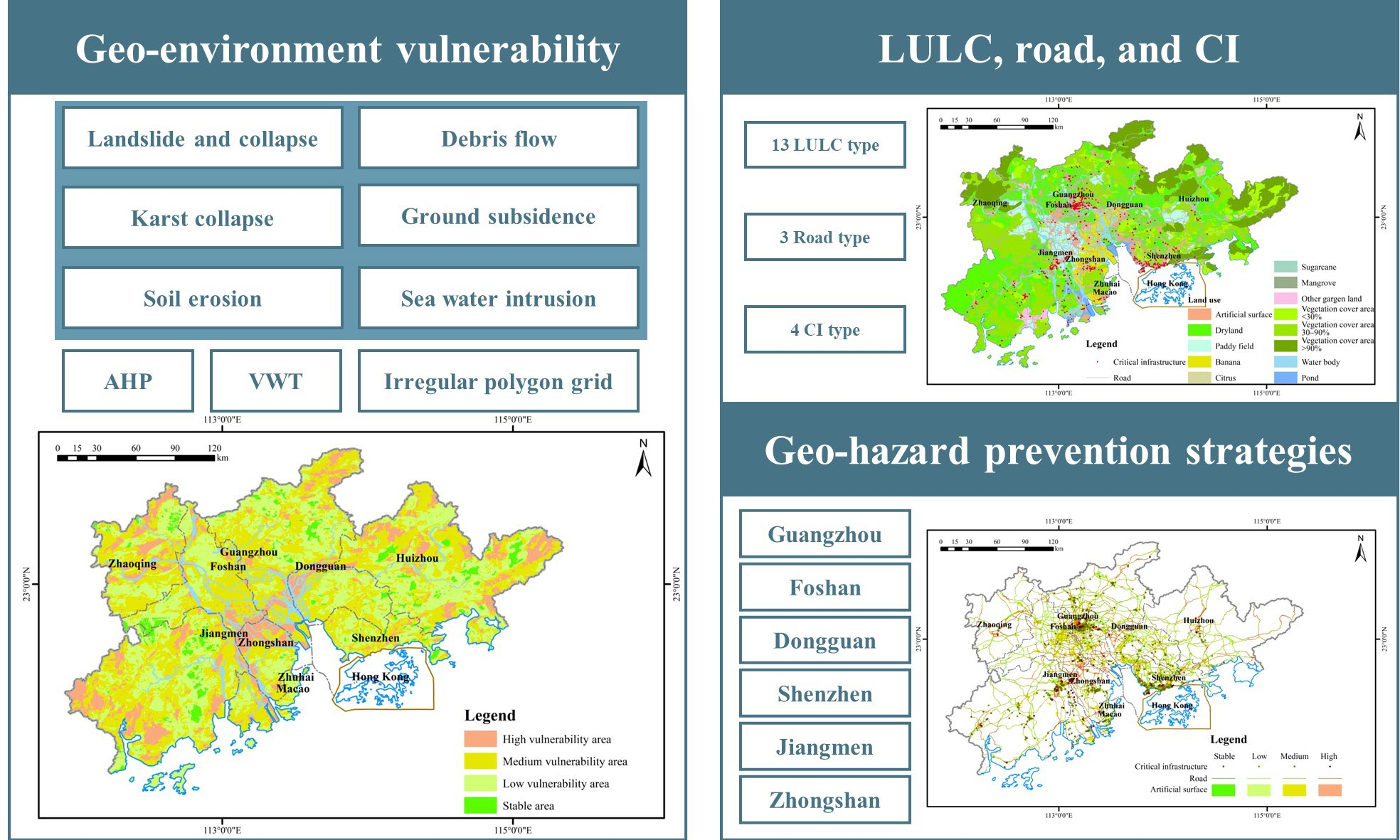
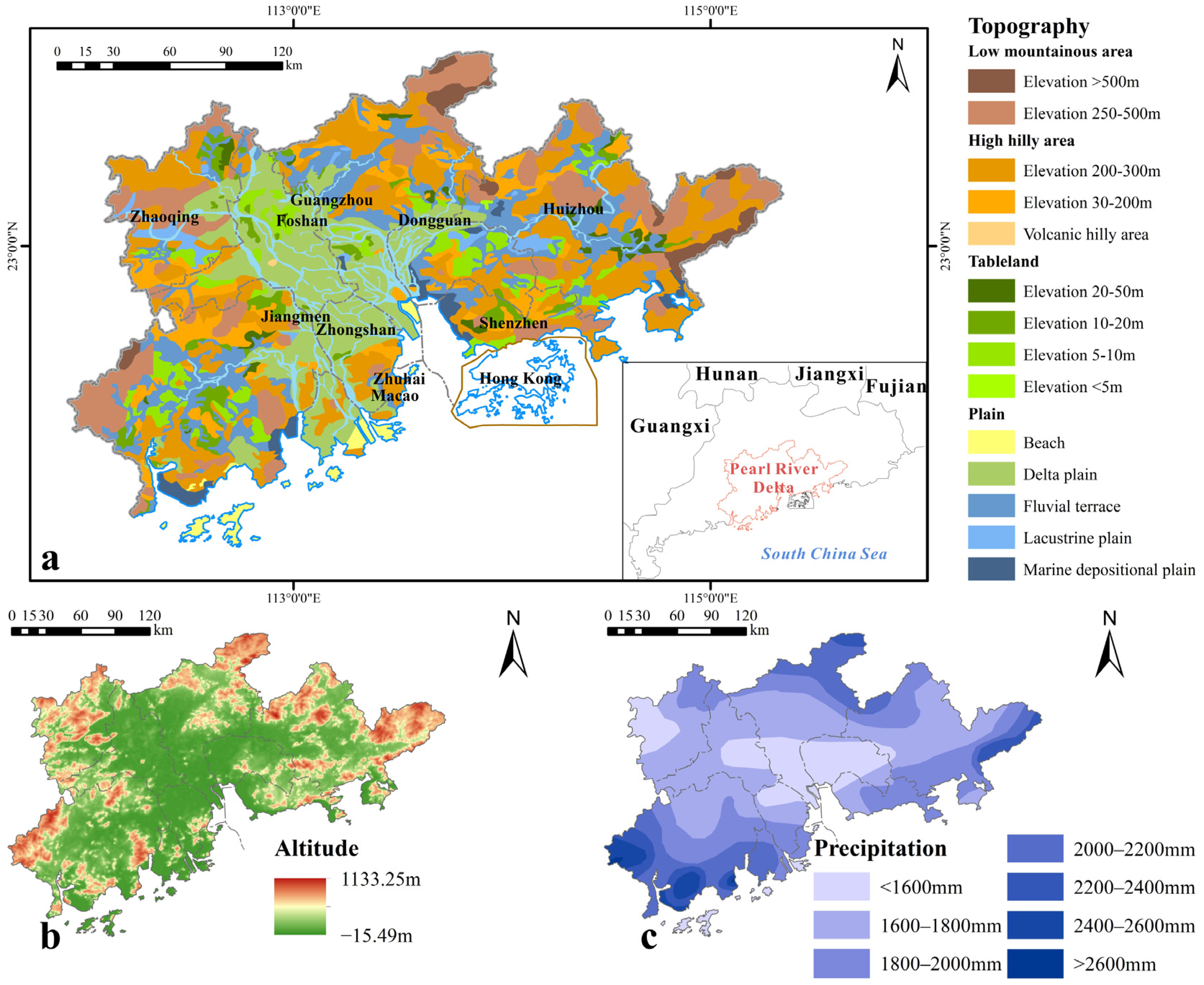
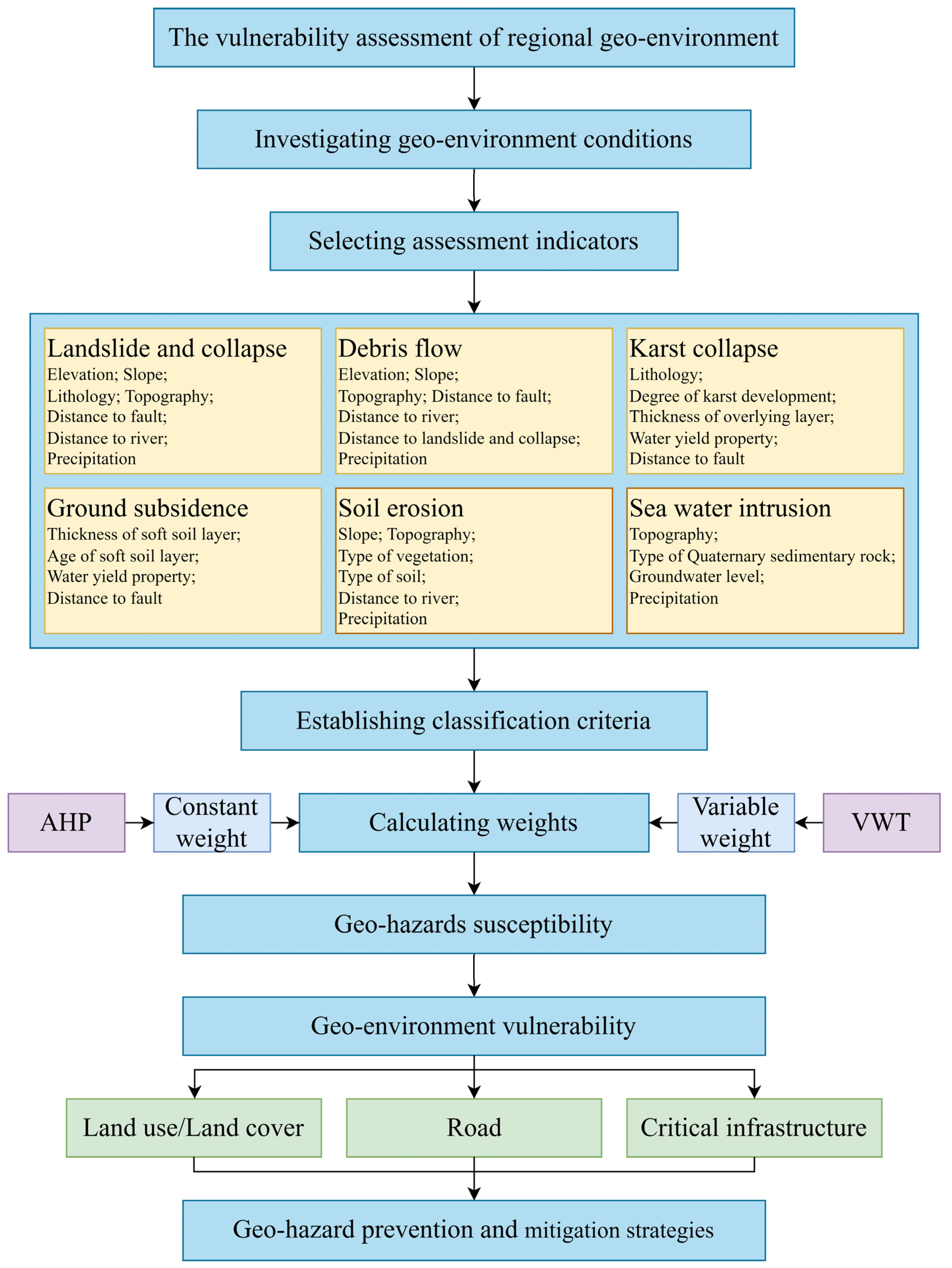
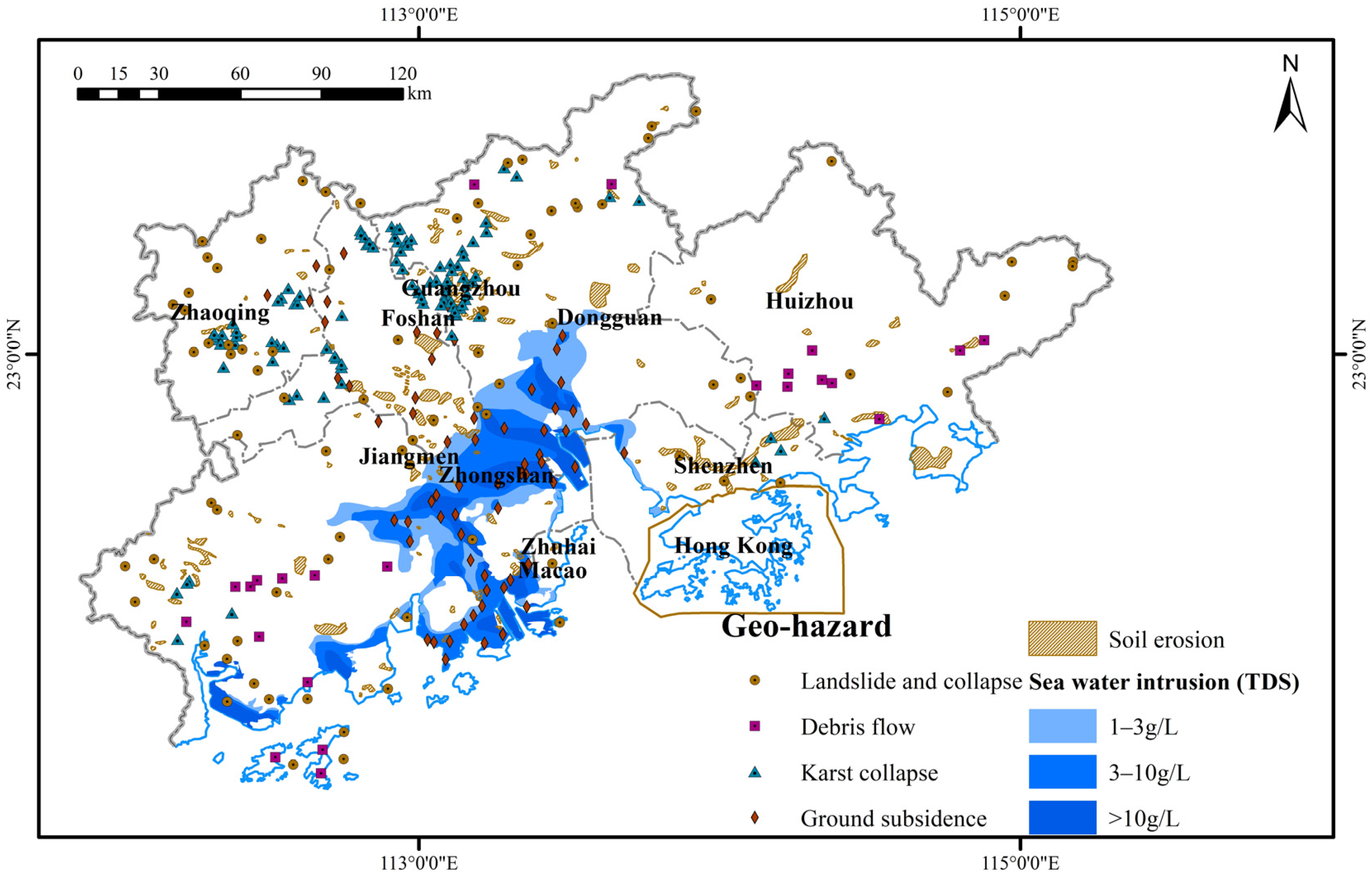
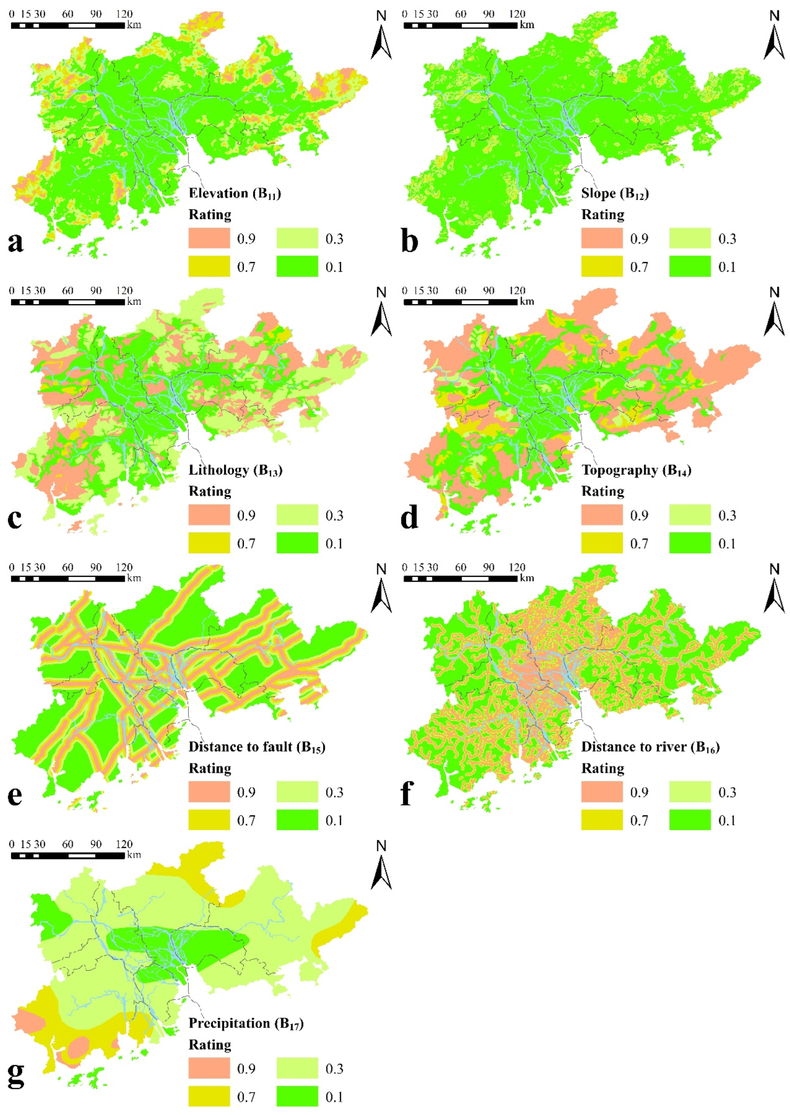
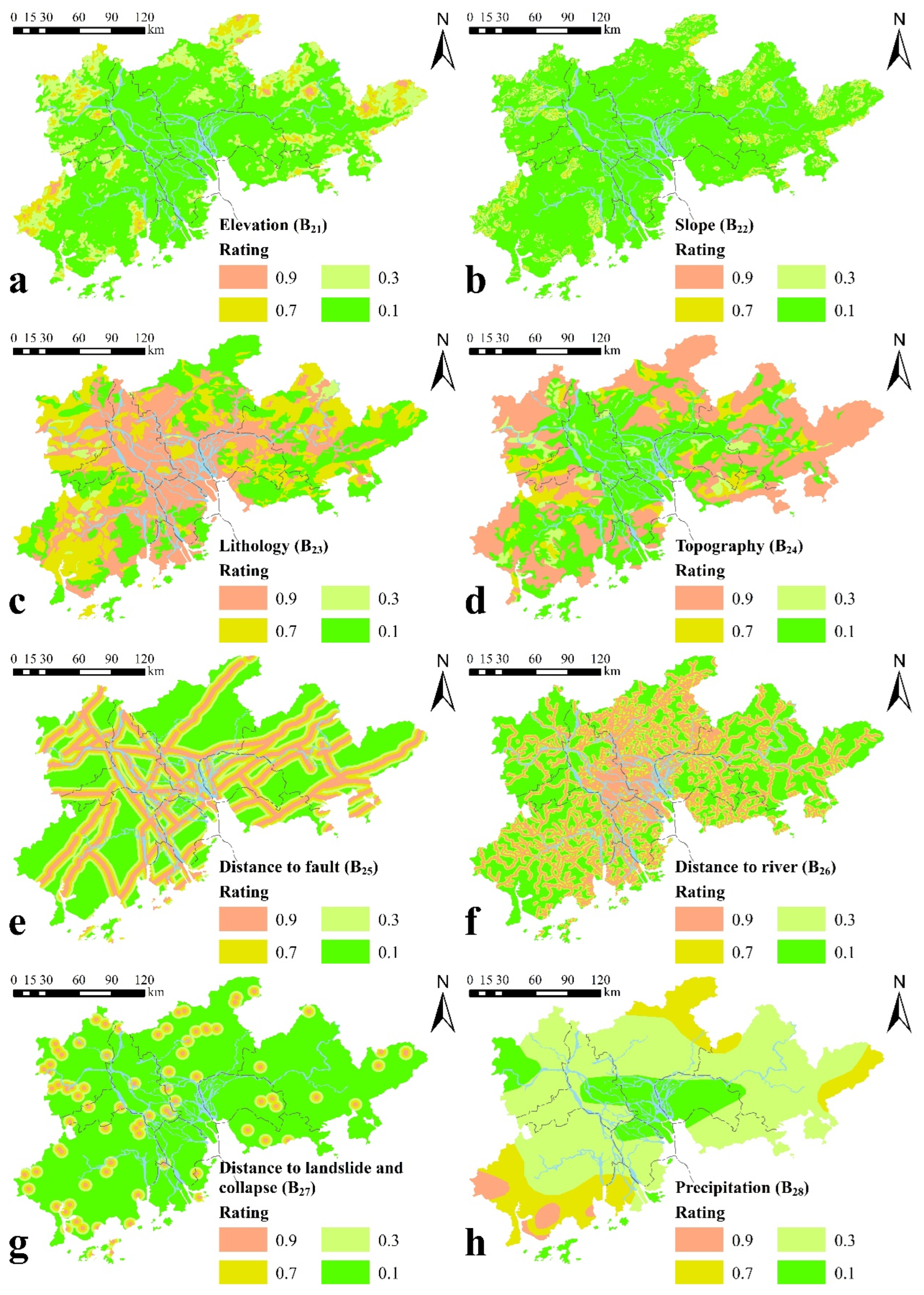
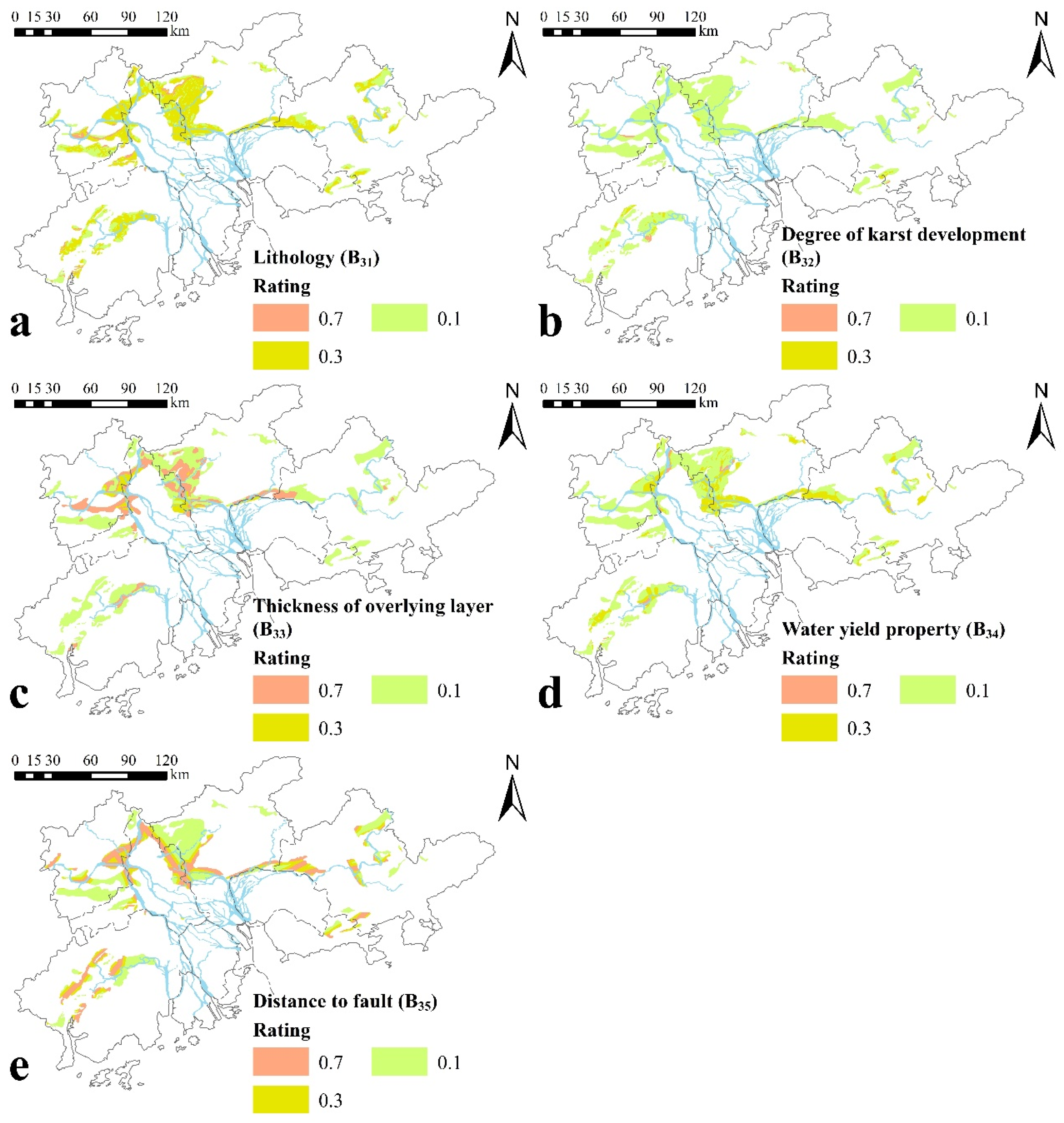
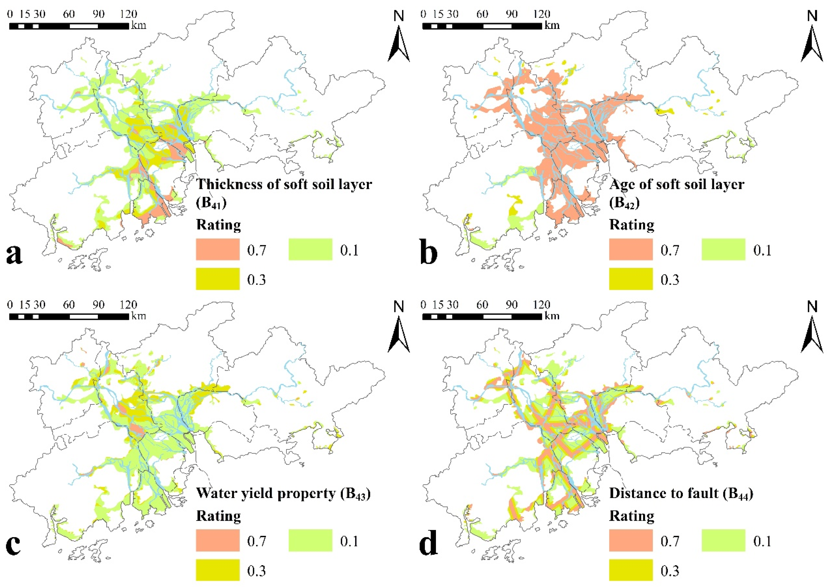
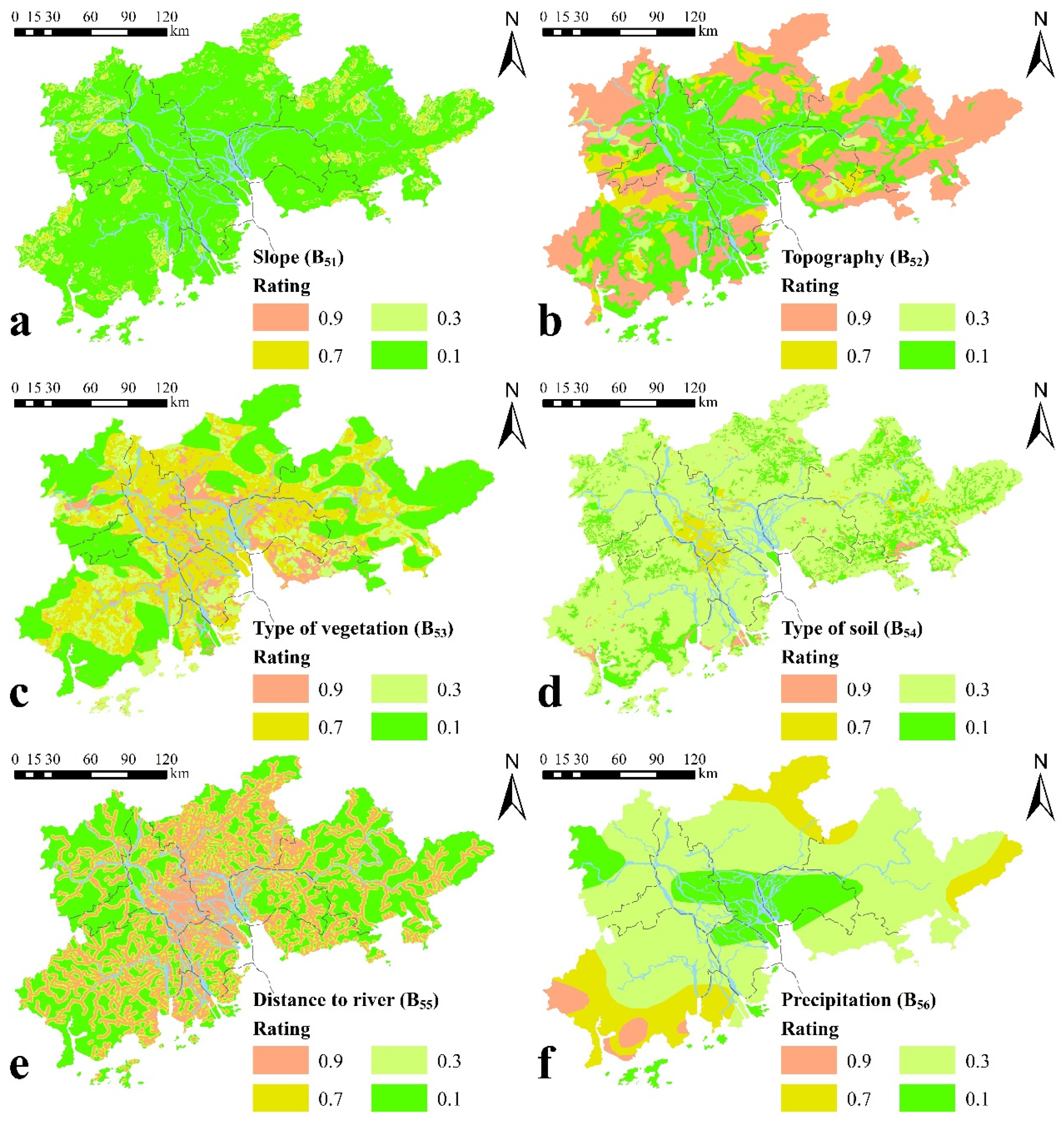
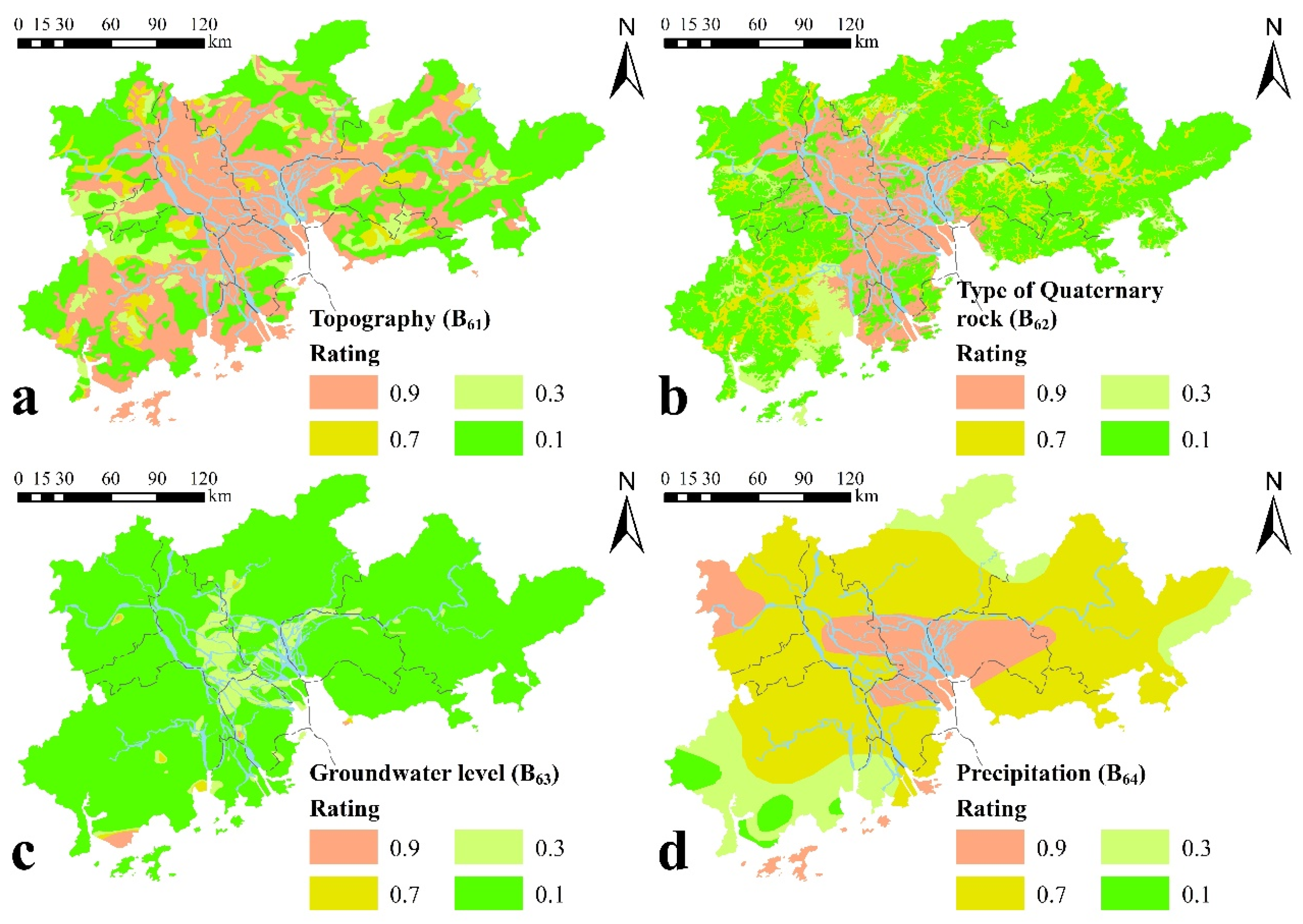
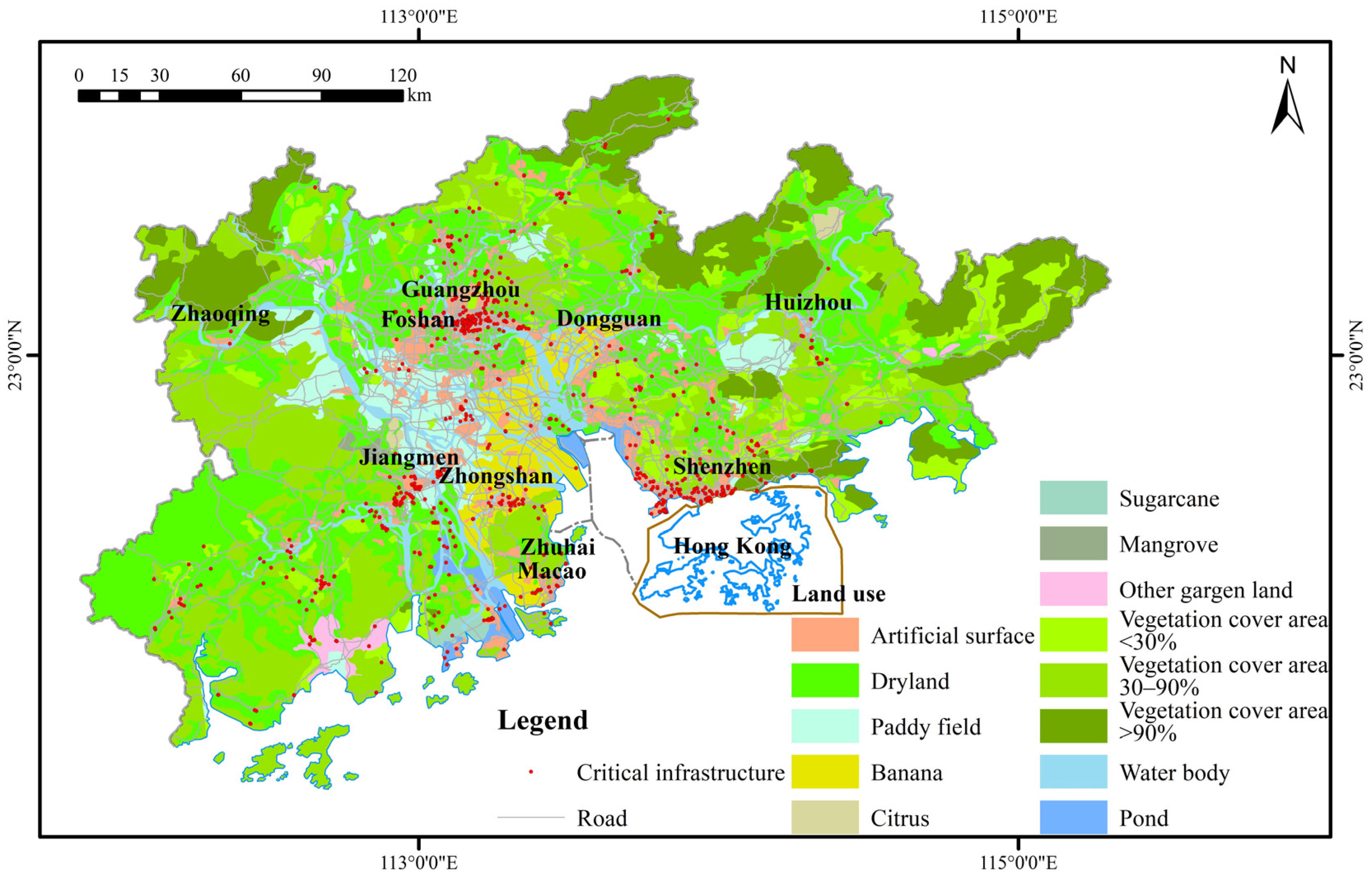
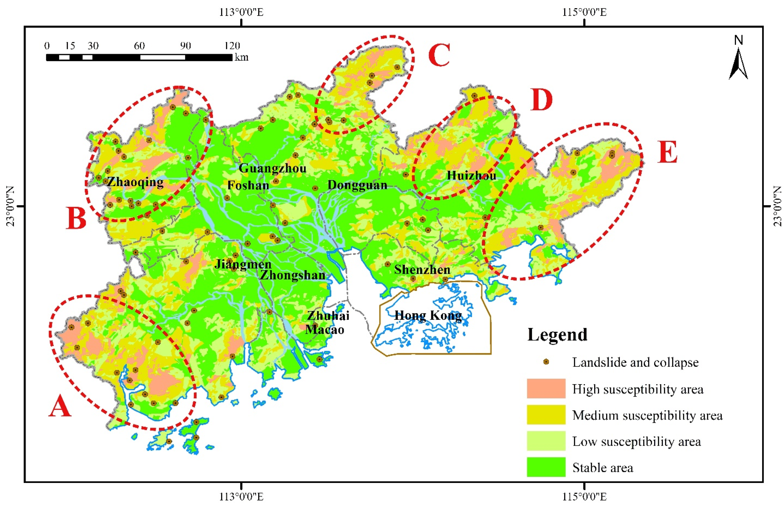
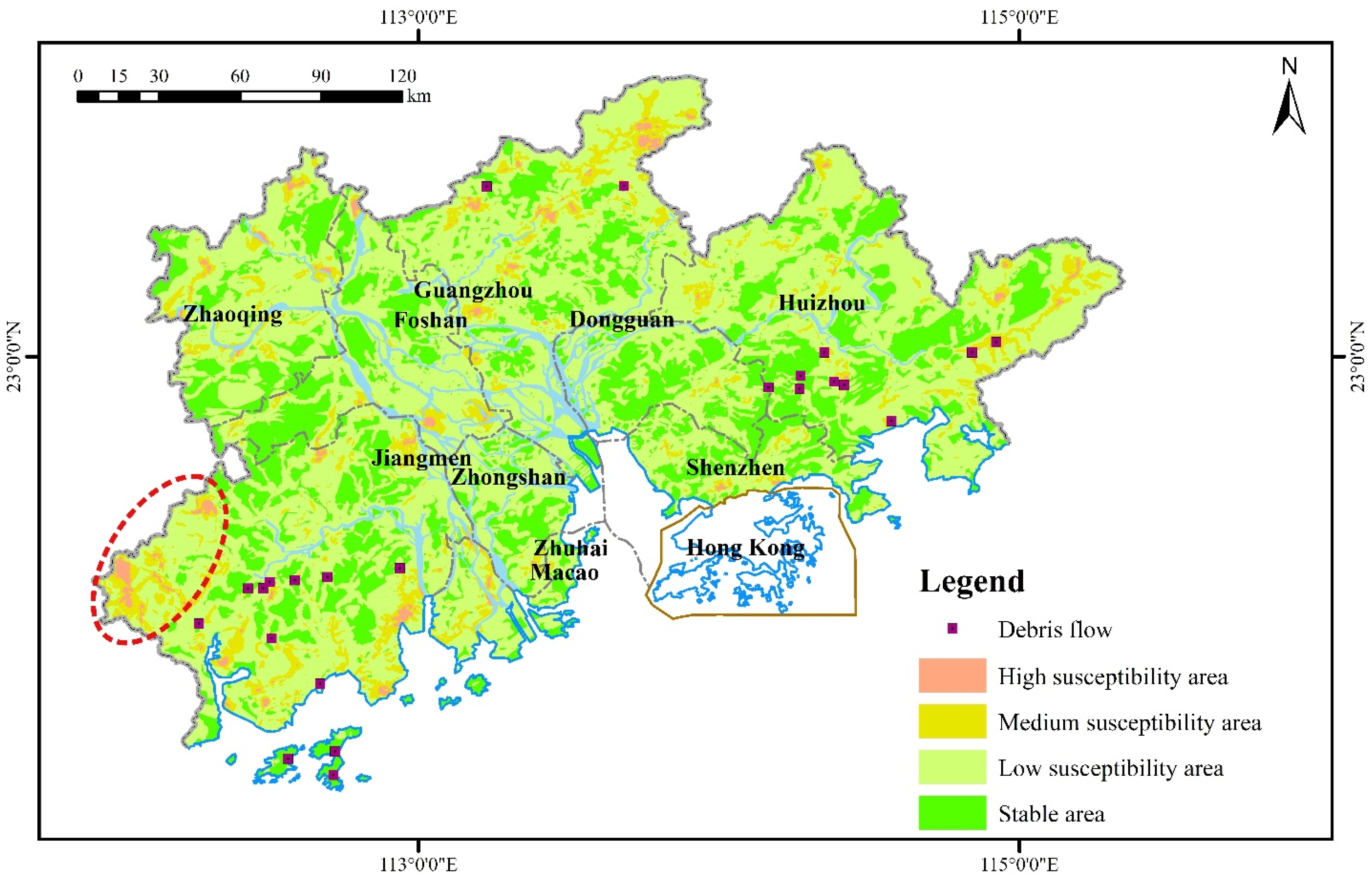
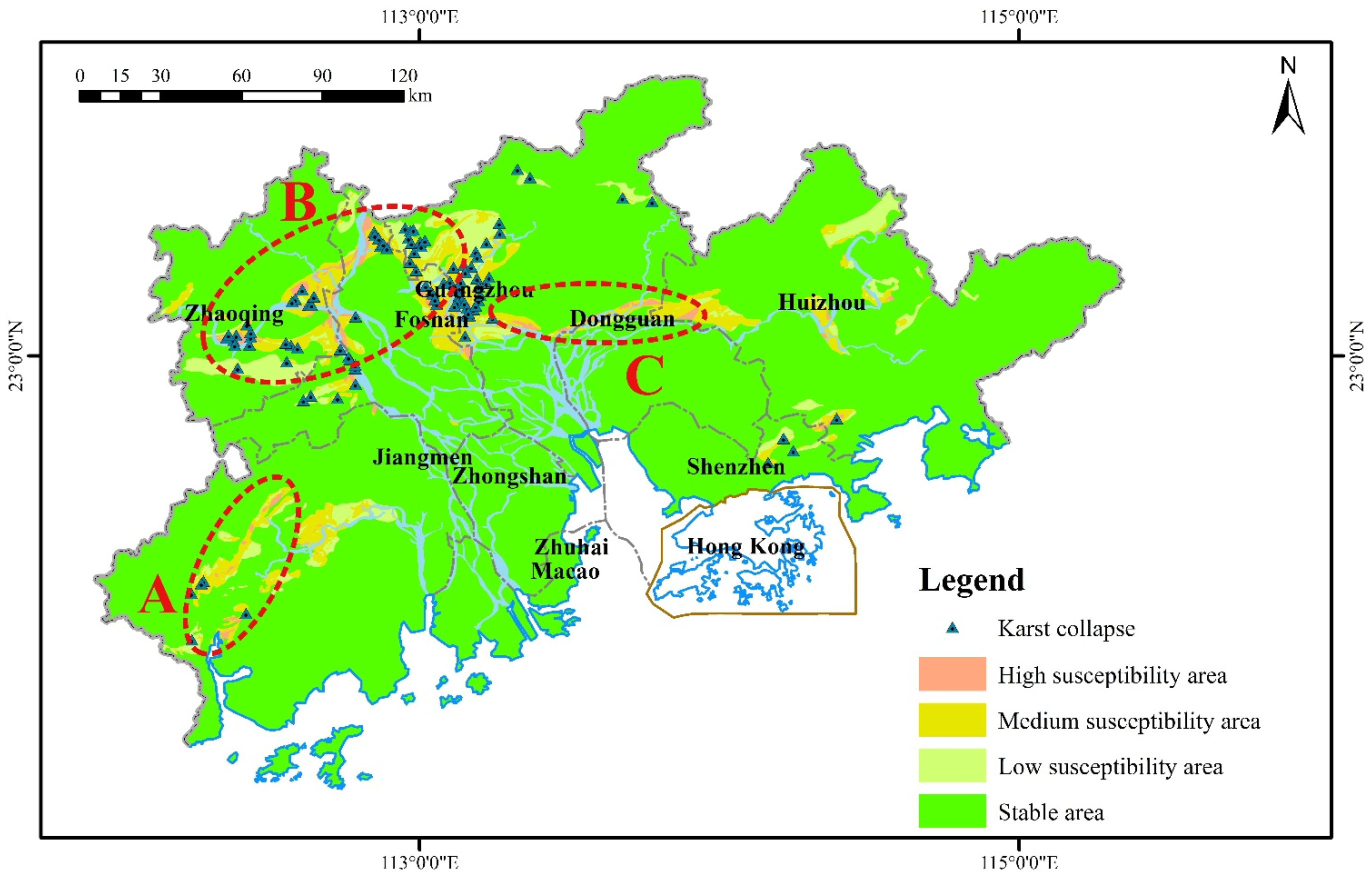
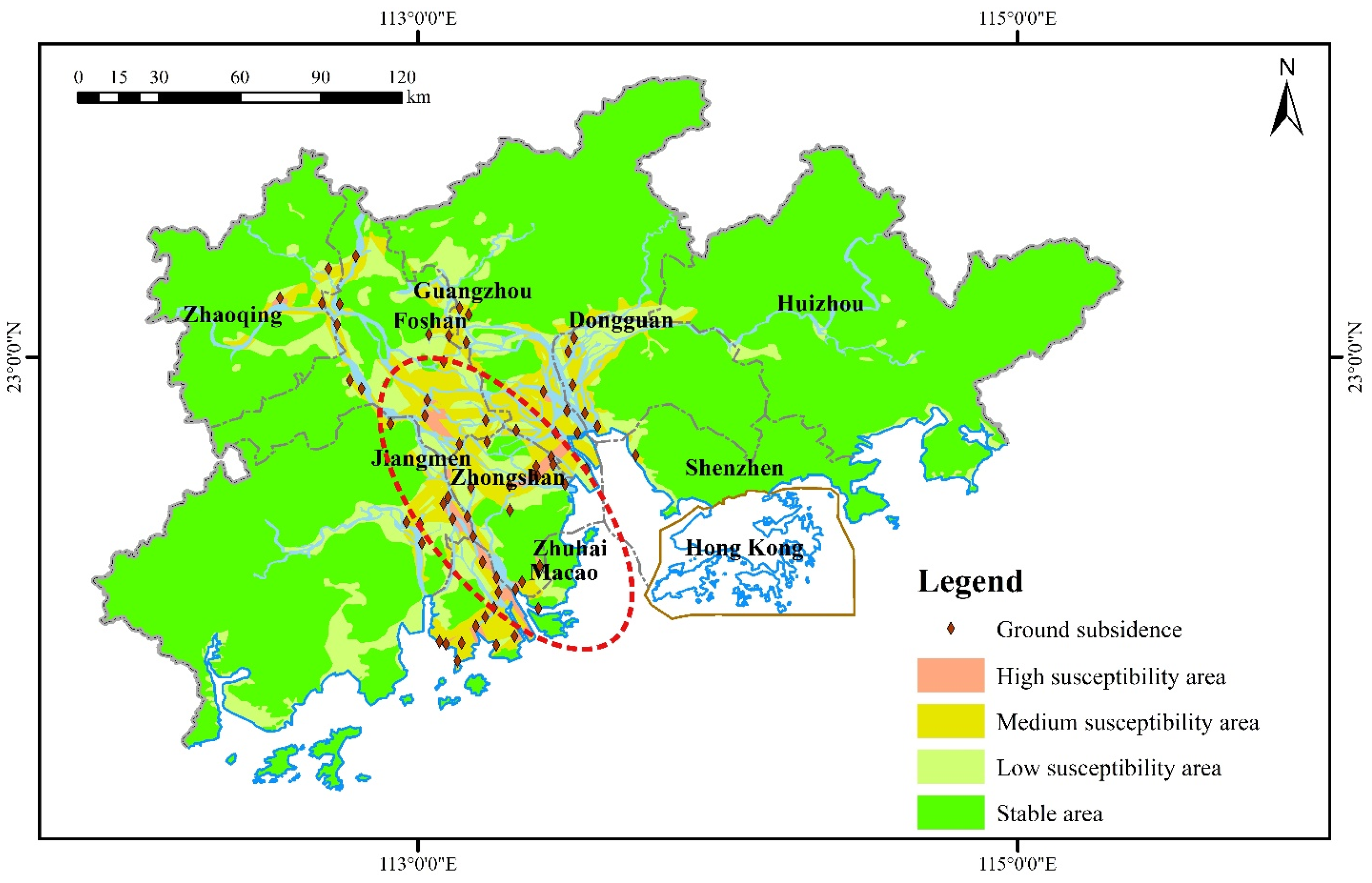
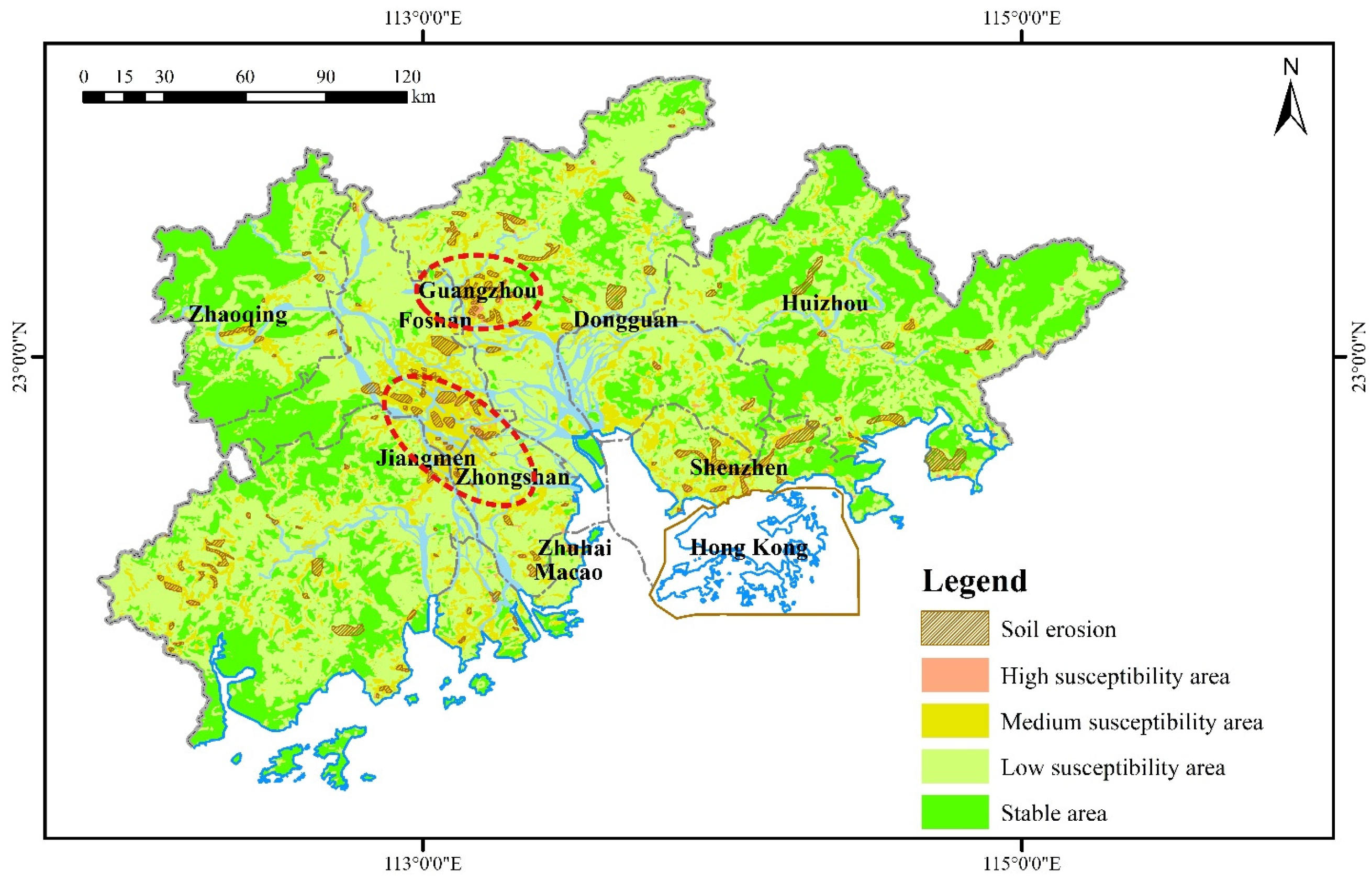
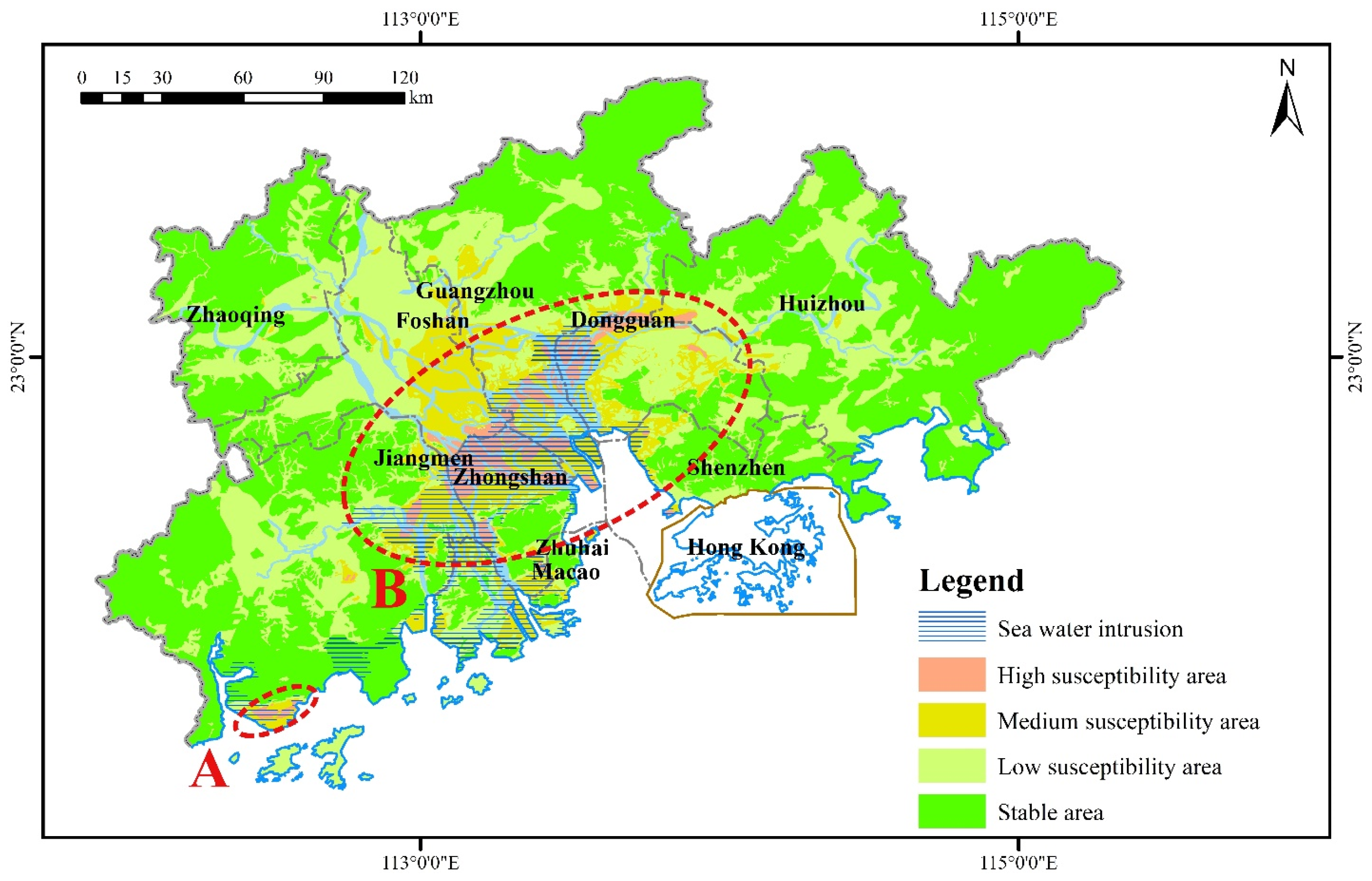
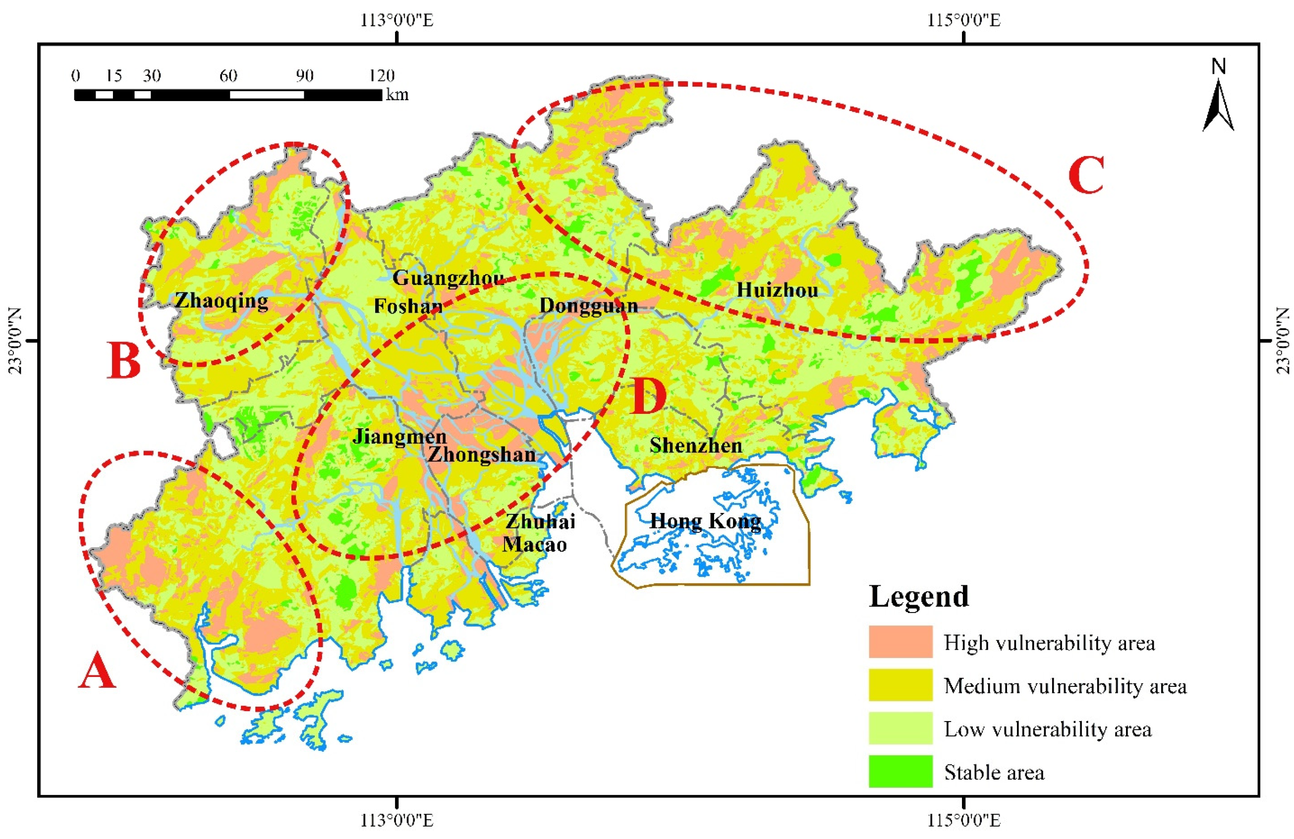
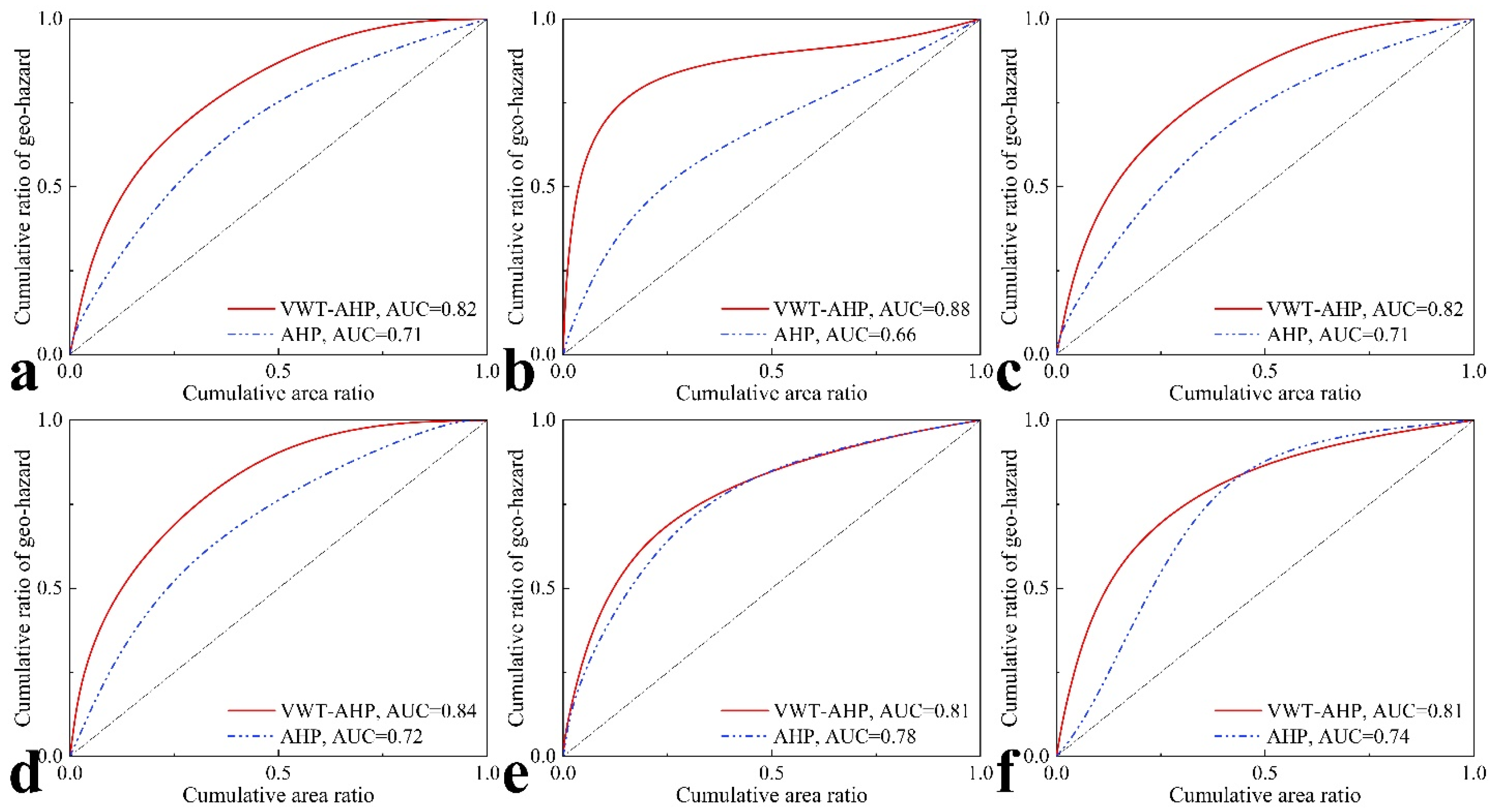
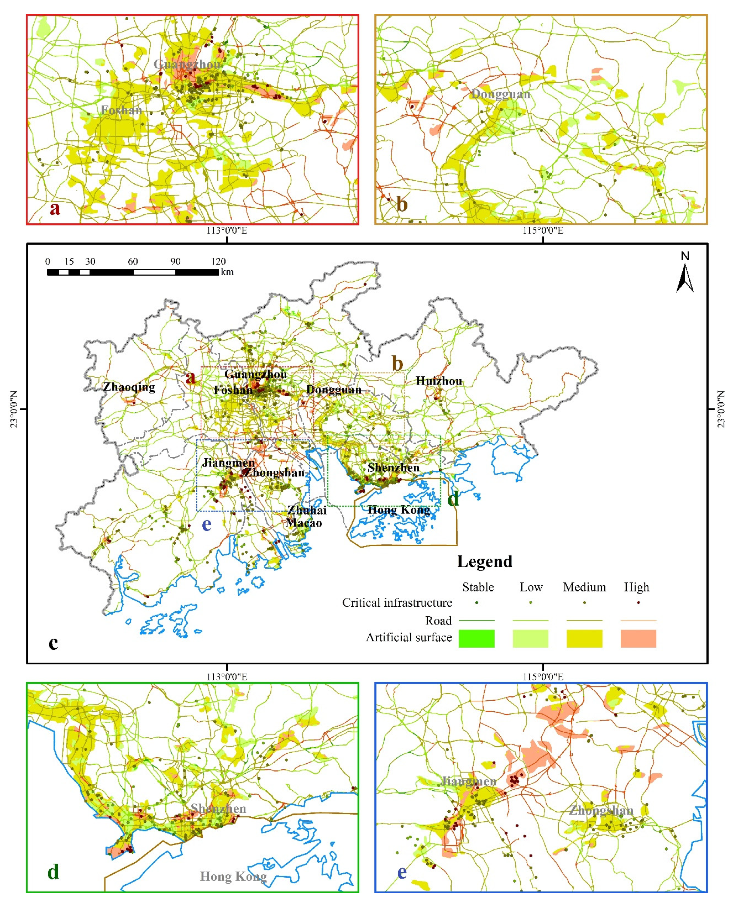
Table 1.
Data types, resolutions, temporal coverages, and sources of all indicators.
| Geohazard Susceptibility | Assessment Indicator | Data Type | Resolution | Temporal Coverage | Source |
|---|---|---|---|---|---|
| Landslide and collapse (A1) | Elevation (B11) | TIFF | 30 m × 30 m | / | Geospatial Data Cloud [59] |
| Slope (B12) | TIFF | 30 m × 30 m | / | / | |
| Lithology (B13) | Shapefile (Polygon) | / | / | Guangdong Geological Survey Institute | |
| Topography (B14) | Shapefile (Polygon) | / | / | Guangdong Geological Survey Institute | |
| Distance to fault (B15) | Shapefile (Polygon) | / | / | Guangdong Geological Survey Institute | |
| Distance to river (B16) | Shapefile (Polygon) | / | 2020 | Google Earth | |
| Precipitation (B17) | Shapefile (Polygon) | / | 2020 | Guangdong Geological Survey Institute | |
| Debris flow (A2) | Elevation (B21) | TIFF | 30 m × 30 m | / | Geospatial Data Cloud [59] |
| Slope (B22) | TIFF | 30 m × 30 m | / | / | |
| Lithology (B23) | Shapefile (Polygon) | / | / | Guangdong Geological Survey Institute | |
| Topography (B24) | Shapefile (Polygon) | / | / | Guangdong Geological Survey Institute | |
| Distance to fault (B25) | Shapefile (Polygon) | / | / | Guangdong Geological Survey Institute | |
| Distance to river (B26) | Shapefile (Polygon) | / | 2020 | Google Earth | |
| Distance to landslide and collapse (B27) | Shapefile (Polygon) | / | / | Guangdong Geological Survey Institute | |
| Precipitation(B28) | Shapefile (Polygon) | / | 2020 | Guangdong Geological Survey Institute | |
| Karst collapse (A3) | Lithology (B31) | Shapefile (Polygon) | / | / | Guangdong Geological Survey Institute |
| Degree of karst development (B32) | Shapefile (Polygon) | / | / | Guangdong Geological Survey Institute | |
| Thickness of overlying layer (B33) | Shapefile (Polygon) | / | / | Guangdong Geological Survey Institute | |
| Water yield property (B34) | Shapefile (Polygon) | / | 2020 | Guangdong Geological Survey Institute | |
| Distance to fault (B35) | Shapefile (Polygon) | / | / | Guangdong Geological Survey Institute | |
| Ground subsidence (A4) | Thickness of soft soil layer (B41) | Shapefile (Polygon) | / | / | Guangdong Geological Survey Institute |
| Age of soft soil layer (B42) | Shapefile (Polygon) | / | / | Guangdong Geological Survey Institute | |
| Water yield property (B43) | Shapefile (Polygon) | / | 2020 | Guangdong Geological Survey Institute | |
| Distance to fault (B44) | Shapefile (Polygon) | / | / | Guangdong Geological Survey Institute | |
| Soil erosion (A5) | Slope (B51) | TIFF | 30 m × 30 m | / | / |
| Topography (B52) | Shapefile (Polygon) | / | / | Guangdong Geological Survey Institute | |
| Type of vegetation (B53) | Shapefile (Polygon) | / | 2020 | Guangdong Geological Survey Institute | |
| Type of soil (B54) | Shapefile (Polygon) | / | 2020 | Soil Science Database [60] | |
| Distance to river (B55) | Shapefile (Polygon) | / | 2020 | Google Earth | |
| Precipitation (B56) | Shapefile (Polygon) | / | 2020 | Guangdong Geological Survey Institute | |
| Sea water intrusion (A6) | Topography (B61) | Shapefile (Polygon) | / | / | Guangdong Geological Survey Institute |
| Type of Quaternary sedimentary rock (B62) | Shapefile (Polygon) | / | / | Guangdong Geological Survey Institute | |
| Groundwater level (B63) | TIFF | 30 m × 30 m | 2020 | Guangdong Geological Survey Institute | |
| Precipitation (B64) | Shapefile (Polygon) | / | 2020 | Guangdong Geological Survey Institute |
Table 2.
Ranges and ratings of all indicators.
| Geohazard Susceptibility | Assessment Indicator | Rating | |||
|---|---|---|---|---|---|
| 0.9 | 0.7 | 0.3 | 0.1 | ||
| Landslide and collapse (A1) | Elevation (B11) | >400 m | 200–400 m | 80–200 m | <80 m |
| Slope (B12) | >20° | 10°–20° | 5°–10° | <5° | |
| Lithology (B13) | Metamorphic rock; clastic rock; sand shale | Carbonate rock; carbonate mudstone | Massive rock; massive lava | Mucky soil; cohesive soil | |
| Topography (B14) | Mountainous area; hilly area (>200 m) | Hilly area (<200 m); volcanic hilly area; tableland (>20 m) | Tableland (10–20 m); lacustrine plain | Tableland (<10 m); beach; fluvial plain; marine depositional plain; delta plain | |
| Distance to fault (B15) | <2 km | 2–4 km | 4–6 km | >6 km | |
| Distance to river (B16) | <0.5 km | 0.5–1 km | 1–1.5 km | >1.5 km | |
| Precipitation (B17) | >2400 mm | 2000–2400 mm | 1600–2000 mm | <1600 mm | |
| Debris flow (A2) | Elevation (B21) | >600 m | 300–600 m | 100–300 m | <100 m |
| Slope (B22) | >20° | 10°–20° | 5°–10° | <5° | |
| Lithology (B23) | Mucky soil; cohesive soil | Metamorphic rock; clastic rock; sand shale | Carbonate rock; carbonate mudstone | Massive rock; massive lava | |
| Topography (B24) | Mountainous area; hilly area (>200 m) | Hilly area (<200 m); volcanic hilly area; tableland (>20 m) | Tableland (10–20 m); lacustrine plain | Tableland (<10 m); beach; fluvial plain; marine depositional plain; delta plain | |
| Distance to fault (B25) | <2 km | 2–4 km | 4–6 km | >6 km | |
| Distance to river (B26) | <0.5 km | 0.5–1 km | 1–1.5 km | >1.5 km | |
| Distance to landslide and collapse (B27) | <2 km | 2–4 km | 4–6 km | >6 km | |
| Precipitation(B28) | >2400 mm | 2000–2400 mm | 1600–2000 mm | <1600 mm | |
| Karst collapse (A3) | Lithology (B31) | / | Carbonate rock | Argillaceous limestone; sandstone; basalt | Mudstone; shale; silly slate |
| Degree of karst development (B32) | / | Strong | Moderate | Poor | |
| Thickness of overlying layer (B33) | / | <10 m | 10–20 m | >20 m | |
| Water yield property (B34) | / | >1000 m3/d | 100–1000 m3/d | <100 m3/d | |
| Distance to fault (B35) | / | <2 km | 2–4 km | >4 km | |
| Ground subsidence (A4) | Thickness of soft soil layer (B41) | / | >20 m | 10–20 m | <10 m |
| Age of soft soil layer (B42) | / | Holocene alluvial deposits; Holocene residual deposits | Holocene Dawanzhen Formation; Holocene Mugao Formation | Holocene Guizhou Formation; Upper Pleistocene deposits | |
| Water yield property (B43) | / | >1000 m3/d | 100–1000 m3/d | <100 m3/d | |
| Distance to fault (B44) | / | <2 km | 2–4 km | >4 km | |
| Soil erosion (A5) | Slope (B51) | >20° | 10°–20° | 5°–10° | <5° |
| Topography (B52) | Mountainous area; hilly area (>200 m) | Hilly area (<200 m); volcanic hilly area; tableland (>20 m) | Tableland (10–20 m); lacustrine plain | Tableland (<10 m); beach; fluvial plain; marine depositional plain; delta plain | |
| Type of vegetation (B53) | Sandy land; urban land | Arable land | Grassland; economic forest land; protective forest land | Arbor land; shrub land | |
| Type of soil (B54) | Latosolic red soil | Alluvial soil | Red soil | Paddy soil | |
| Distance to river (B55) | <0.5 km | 0.5–1 km | 1–1.5 km | >1.5 km | |
| Precipitation (B56) | >2400 mm | 2000–2400 mm | 1600–2000 mm | <1600 mm | |
| Sea water intrusion (A6) | Topography (B61) | Tableland (<10 m); beach; fluvial plain; marine depositional plain; delta plain | Tableland (10–20 m); lacustrine plain | Hilly area (<200 m); volcanic hilly area; tableland (>20 m) | Mountainous area; hilly area (>200 m) |
| Type of Quaternary sedimentary rock (B62) | Alluvial sandy clay | Marine clay | Proluvial clay | Bedrock | |
| Groundwater level (B63) | <−2 m | −2–0 m | 0–2 m | >2 m | |
| Precipitation (B64) | <1600 mm | 1600–2000 mm | 2000–2400 mm | >2400 mm | |
Table 3.
Pairwise comparison scale for AHP.
| Scale | 1 | 3 | 5 | 7 | 9 |
|---|---|---|---|---|---|
| Importance | Equal | Moderate | Strong | Very strong | Extreme |
Table 4.
Average Random Consistency Index.
| n | 1 | 2 | 3 | 4 | 5 | 6 | 7 | 8 | 9 | 10 |
|---|---|---|---|---|---|---|---|---|---|---|
| RI | 0 | 0 | 0.52 | 0.89 | 1.11 | 1.24 | 1.35 | 1.40 | 1.45 | 1.49 |
Table 5.
Results of susceptibility assessment of geohazards.
| Geohazard | Method | Area | Stable | Low | Medium | High |
|---|---|---|---|---|---|---|
| Landslide and collapse | VWT-AHP | Area (km2) | 18,645.75 | 9688.68 | 9848.89 | 3514.68 |
| Number of geohazards | 3 | 3 | 22 | 56 | ||
| Density of geohazards | 0.0002 | 0.0003 | 0.0022 | 0.0159 | ||
| AHP | Area (km2) | 20,079.53 | 11,597.94 | 8076.18 | 1944.34 | |
| Number of geohazards | 8 | 25 | 37 | 13 | ||
| Density of geohazards | 0.0004 | 0.0022 | 0.0046 | 0.0067 | ||
| Debris flow | VWT-AHP | Area (km2) | 10,692.25 | 26,905.16 | 3619.66 | 480.94 |
| Number of geohazards | 2 | 1 | 11 | 9 | ||
| Density of geohazards | 0.0002 | 0.0000 | 0.0030 | 0.0187 | ||
| AHP | Area (km2) | 14,253.97 | 19,483.31 | 6716.05 | 1244.67 | |
| Number of geohazards | 5 | 6 | 9 | 3 | ||
| Density of geohazards | 0.0004 | 0.0003 | 0.0013 | 0.0024 | ||
| Karst collapse | VWT-AHP | Area (km2) | 36,841.23 | 1812.95 | 2553.61 | 484.94 |
| Number of geohazards | 0 | 1 | 39 | 57 | ||
| Density of geohazards | 0.0000 | 0.0006 | 0.0153 | 0.1175 | ||
| AHP | Area (km2) | 36,841.23 | 3033.69 | 1752.37 | 65.42 | |
| Number of geohazards | 0 | 24 | 62 | 11 | ||
| Density of geohazards | 0.0000 | 0.0079 | 0.0354 | 0.1681 | ||
| Ground subsidence | VWT-AHP | Area (km2) | 33,007.04 | 4468.67 | 3741.2 | 454.65 |
| Number of geohazards | 0 | 1 | 33 | 31 | ||
| Density of geohazards | 0.0000 | 0.0002 | 0.0088 | 0.0682 | ||
| AHP | Area (km2) | 33,007.04 | 1109.03 | 5616.46 | 1939.02 | |
| Number of geohazards | 0 | 0 | 25 | 40 | ||
| Density of geohazards | 0.0000 | 0.0000 | 0.0045 | 0.0206 | ||
| Soil erosion | VWT-AHP | Area (km2) | 13,081.98 | 22,743.83 | 5526.97 | 344.54 |
| Area of geohazards (km2) | 71.96 | 252.77 | 627.08 | 133.84 | ||
| Density of geohazards | 0.0055 | 0.0111 | 0.1135 | 0.3885 | ||
| AHP | Area (km2) | 14,525.31 | 15,470.48 | 10,386.07 | 1315.47 | |
| Area of geohazards (km2) | 81.36 | 180.78 | 548.36 | 275.17 | ||
| Density of geohazards | 0.0056 | 0.0117 | 0.0528 | 0.2092 | ||
| Sea water intrusion | VWT-AHP | Area (km2) | 22,136.74 | 14,123.59 | 4341.74 | 1095.33 |
| Area of geohazards (km2) | 471.08 | 1277.44 | 1893.99 | 889.54 | ||
| Density of geohazards | 0.0213 | 0.0904 | 0.4362 | 0.8121 | ||
| AHP | Area (km2) | 20,285.86 | 9269.77 | 8698.65 | 3443.12 | |
| Area of geohazards (km2) | 196.89 | 846.61 | 1875 | 413.55 | ||
| Density of geohazards | 0.0097 | 0.0913 | 0.2156 | 0.1201 |
Table 6.
Results of single-indicator sensitivity analysis.
| Geohazard Susceptibility | Assessment Indicator | Maximum | Minimum | Average | Standard Deviation |
|---|---|---|---|---|---|
| Landslide and collapse (A1) | Elevation (B11) | 0.6089 | 0.0133 | 0.1004 | 0.0877 |
| Slope (B12) | 0.4058 | 0.0106 | 0.0492 | 0.0371 | |
| Lithology (B13) | 0.8187 | 0.0280 | 0.2413 | 0.1969 | |
| Topography (B14) | 0.6304 | 0.0096 | 0.1844 | 0.1407 | |
| Distance to fault (B15) | 0.6512 | 0.0100 | 0.1453 | 0.1435 | |
| Distance to river (B16) | 0.4906 | 0.0059 | 0.0952 | 0.0904 | |
| Precipitation (B17) | 0.8034 | 0.0218 | 0.1842 | 0.1232 | |
| Debris flow (A2) | Elevation (B21) | 0.3267 | 0.0063 | 0.0403 | 0.0383 |
| Slope (B22) | 0.3539 | 0.0069 | 0.0318 | 0.0267 | |
| Lithology (B23) | 0.6452 | 0.0112 | 0.1638 | 0.1372 | |
| Topography (B24) | 0.6646 | 0.0135 | 0.2371 | 0.1696 | |
| Distance to fault (B25) | 0.5780 | 0.0080 | 0.1008 | 0.0990 | |
| Distance to river (B26) | 0.7111 | 0.0162 | 0.1680 | 0.1411 | |
| Distance to landslide and collapse (B27) | 0.7722 | 0.0206 | 0.0960 | 0.1028 | |
| Precipitation(B28) | 0.7722 | 0.0207 | 0.1621 | 0.1123 | |
| Karst collapse (A3) | Lithology (B31) | 0.7268 | 0.0603 | 0.2707 | 0.1429 |
| Degree of karst development (B32) | 0.7268 | 0.0587 | 0.1748 | 0.0946 | |
| Thickness of overlying layer (B33) | 0.4356 | 0.0161 | 0.1288 | 0.1149 | |
| Water yield property (B34) | 0.4356 | 0.0178 | 0.0852 | 0.0531 | |
| Distance to fault (B35) | 0.6833 | 0.0491 | 0.3405 | 0.1852 | |
| Ground subsidence (A4) | Thickness of soft soil layer (B41) | 0.7917 | 0.0747 | 0.1872 | 0.1114 |
| Age of soft soil layer (B42) | 0.7683 | 0.1054 | 0.5342 | 0.1878 | |
| Water yield property (B43) | 0.4935 | 0.0203 | 0.0826 | 0.0690 | |
| Distance to fault (B44) | 0.6223 | 0.0376 | 0.1960 | 0.1396 | |
| Soil erosion (A5) | Slope (B51) | 0.3794 | 0.0077 | 0.0398 | 0.0356 |
| Topography (B52) | 0.5837 | 0.0082 | 0.1825 | 0.1612 | |
| Type of vegetation (B53) | 0.8482 | 0.0295 | 0.3052 | 0.2061 | |
| Type of soil (B54) | 0.8290 | 0.0305 | 0.1728 | 0.1076 | |
| Distance to river (B55) | 0.7106 | 0.0152 | 0.2072 | 0.1488 | |
| Precipitation (B56) | 0.6175 | 0.0089 | 0.0925 | 0.0765 | |
| Sea water intrusion (A6) | Topography (B61) | 0.6626 | 0.0155 | 0.2534 | 0.1756 |
| Type of Quaternary sedimentary rock (B62) | 0.7534 | 0.0240 | 0.2046 | 0.1731 | |
| Groundwater level (B63) | 0.8753 | 0.0496 | 0.1346 | 0.0829 | |
| Precipitation (B64) | 0.8054 | 0.0270 | 0.4074 | 0.1521 |
Table 7.
Distribution of critical infrastructures, roads, and artificial surfaces in different vulnerability areas.
Table 7.
Distribution of critical infrastructures, roads, and artificial surfaces in different vulnerability areas.
| Stable | Low | Medium | High | |
|---|---|---|---|---|
| Critical infrastructure | 8 | 175 | 512 | 102 |
| Road (km) | 575.43 | 10,258.47 | 16,550.36 | 3890.09 |
| Artificial surface (km2) | 18.95 | 447.95 | 1653.15 | 359.71 |
Disclaimer/Publisher’s Note: The statements, opinions and data contained in all publications are solely those of the individual author(s) and contributor(s) and not of MDPI and/or the editor(s). MDPI and/or the editor(s) disclaim responsibility for any injury to people or property resulting from any ideas, methods, instructions or products referred to in the content. |
© 2023 by the authors. Licensee MDPI, Basel, Switzerland. This article is an open access article distributed under the terms and conditions of the Creative Commons Attribution (CC BY) license (https://creativecommons.org/licenses/by/4.0/).
Share and Cite
MDPI and ACS Style
Huang, P.; Wu, X.; Ma, C.; Zhou, A. Geo-Environment Vulnerability Assessment of Multiple Geohazards Using VWT-AHP: A Case Study of the Pearl River Delta, China. Remote Sens. 2023, 15, 5007. https://doi.org/10.3390/rs15205007
AMA Style
Huang P, Wu X, Ma C, Zhou A. Geo-Environment Vulnerability Assessment of Multiple Geohazards Using VWT-AHP: A Case Study of the Pearl River Delta, China. Remote Sensing. 2023; 15(20):5007. https://doi.org/10.3390/rs15205007
Chicago/Turabian StyleHuang, Peng, Xiaoyu Wu, Chuanming Ma, and Aiguo Zhou. 2023. "Geo-Environment Vulnerability Assessment of Multiple Geohazards Using VWT-AHP: A Case Study of the Pearl River Delta, China" Remote Sensing 15, no. 20: 5007. https://doi.org/10.3390/rs15205007
Note that from the first issue of 2016, this journal uses article numbers instead of page numbers. See further details here.