
Mapping Coastal Wetlands and Their Dynamics in the Yellow River Delta over Last Three Decades: Based on a Spectral Endmember Space
 ,
,  and
and
Abstract
:1. Introduction
2. Materials
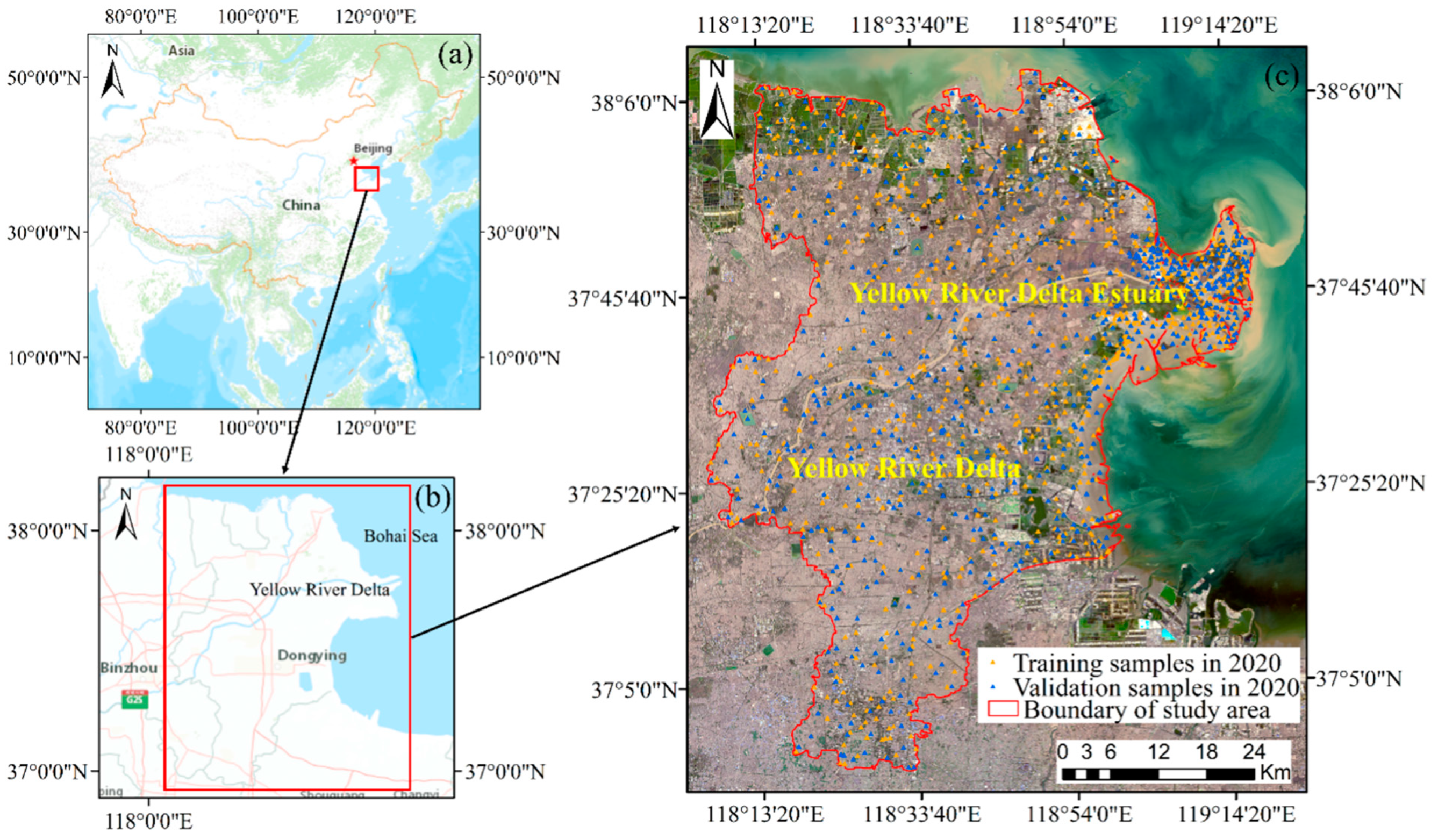
2.1. Study Area
2.2. Data Sources and Pre-Processing
2.2.1. Remote Sensing Data
2.2.2. Training and Validation Samples
3. Methods
3.1. Coastal Wetland Classification System
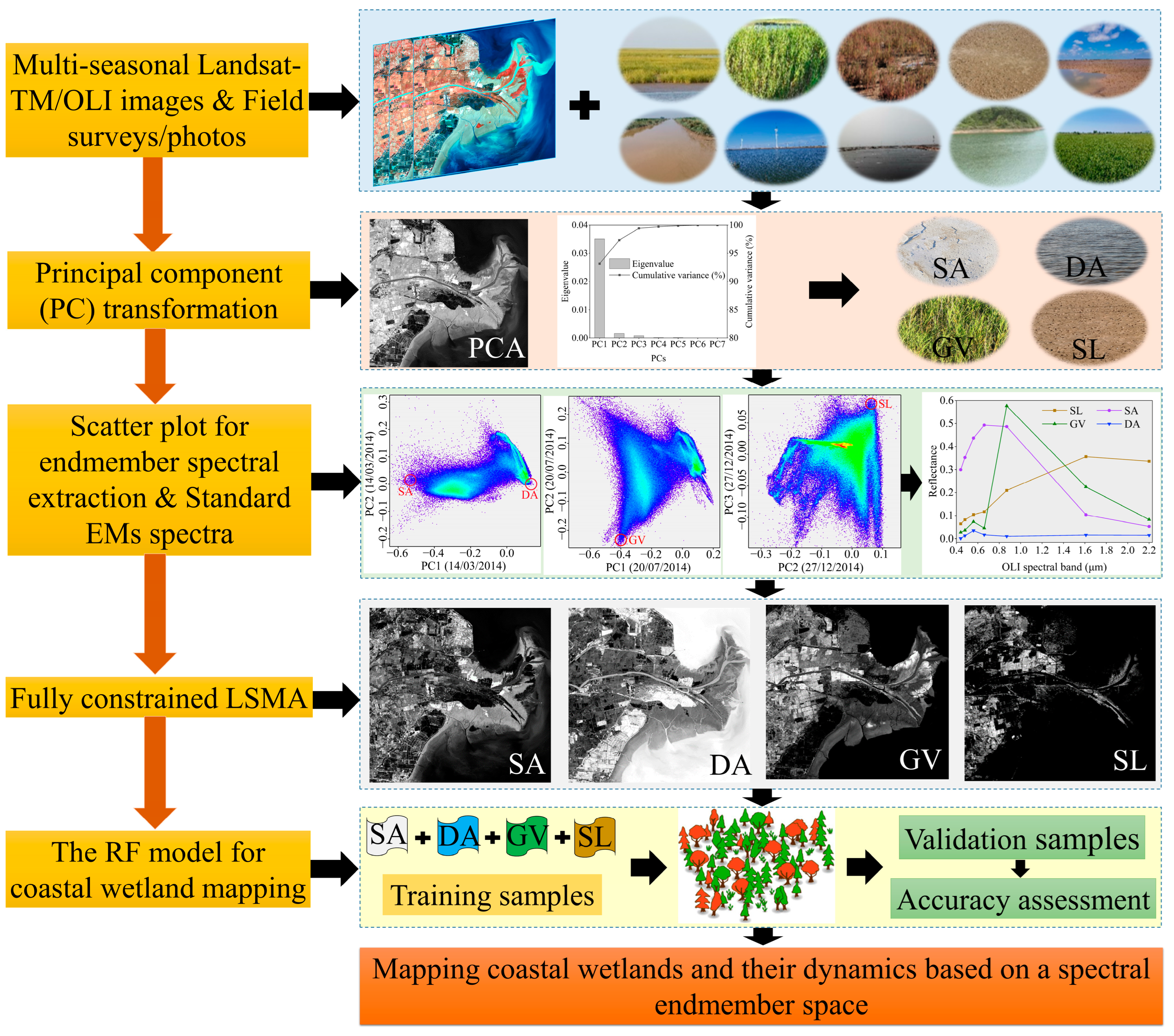
3.2. The Methods of Coastal Wetland Mapping
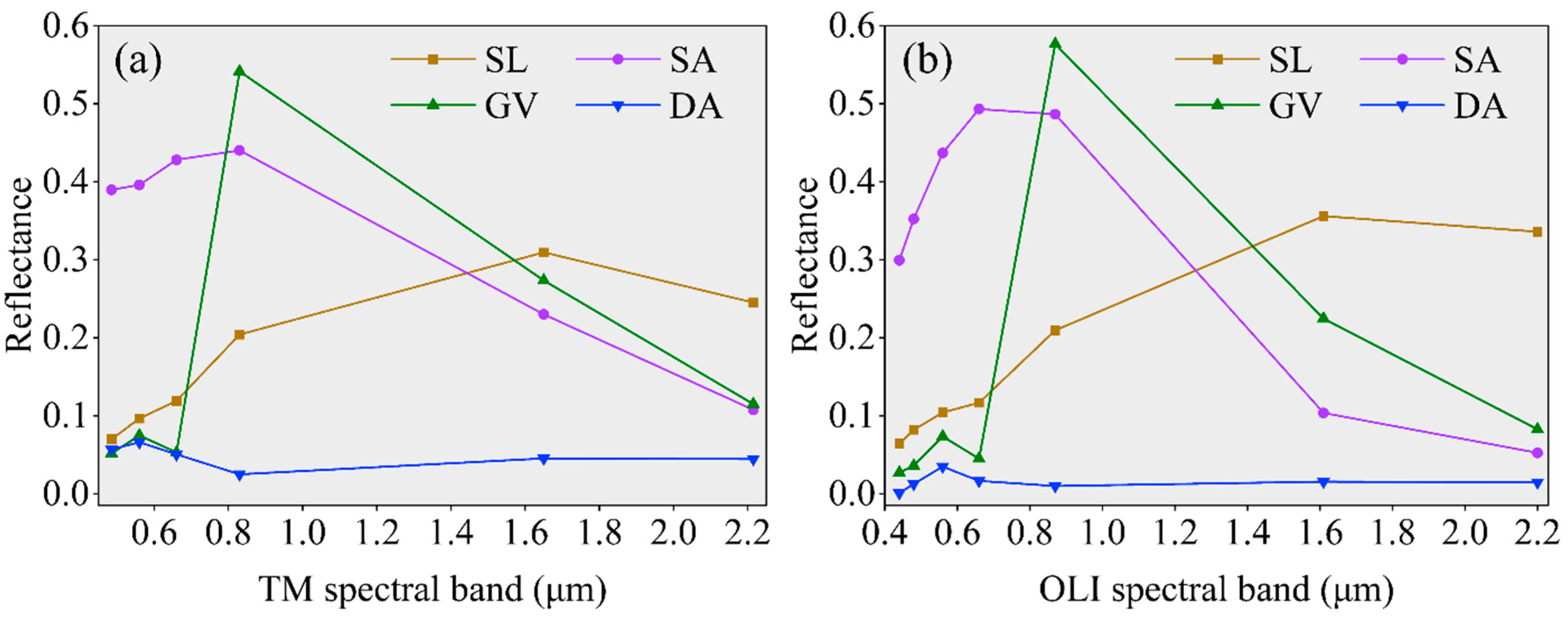
3.2.1. Linear Spectral Mixture Analysis (LSMA)
3.2.2. Mapping Costal Wetland
3.3. Mapping Accuracy Assessment
3.4. Landscape Indices of Coastal Wetlands
4. Results
4.1. Accuracy Assessment of Coastal Wetland Mapping
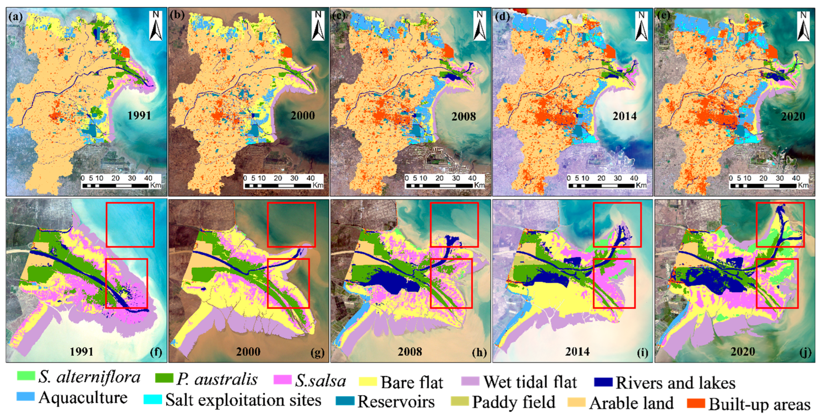
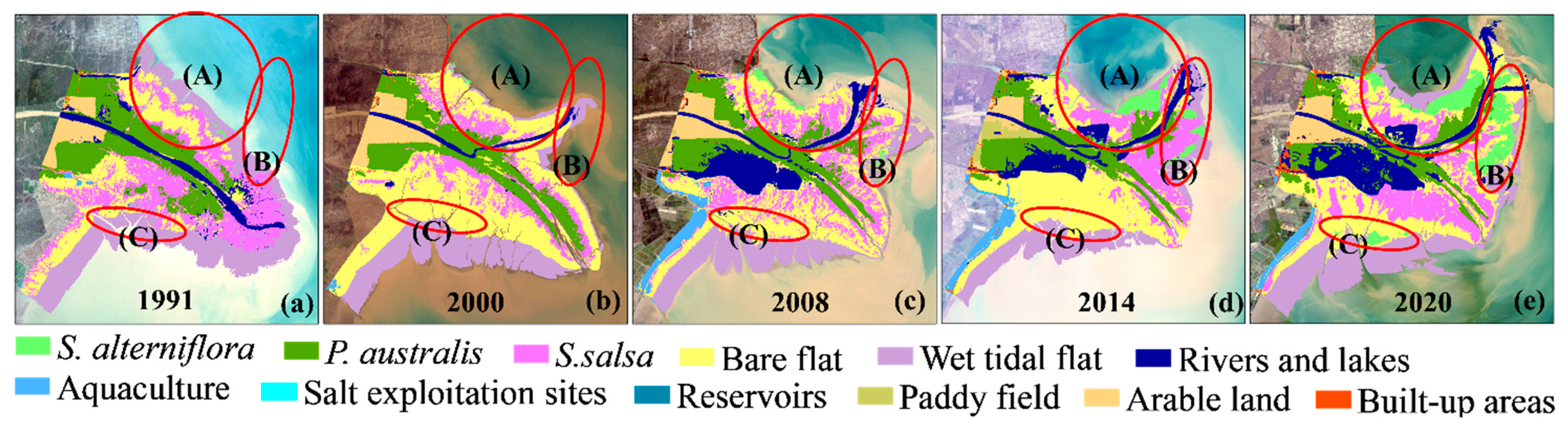
4.2. Coastal Wetland Dynamics during 1991–2020 in the YRD
4.3. The Evolution Dynamics of Different Wetland Vegetation in the YRD Estuary
4.4. Bare Flat and Human-Made Wetland Dynamics in the YRD
5. Discussion
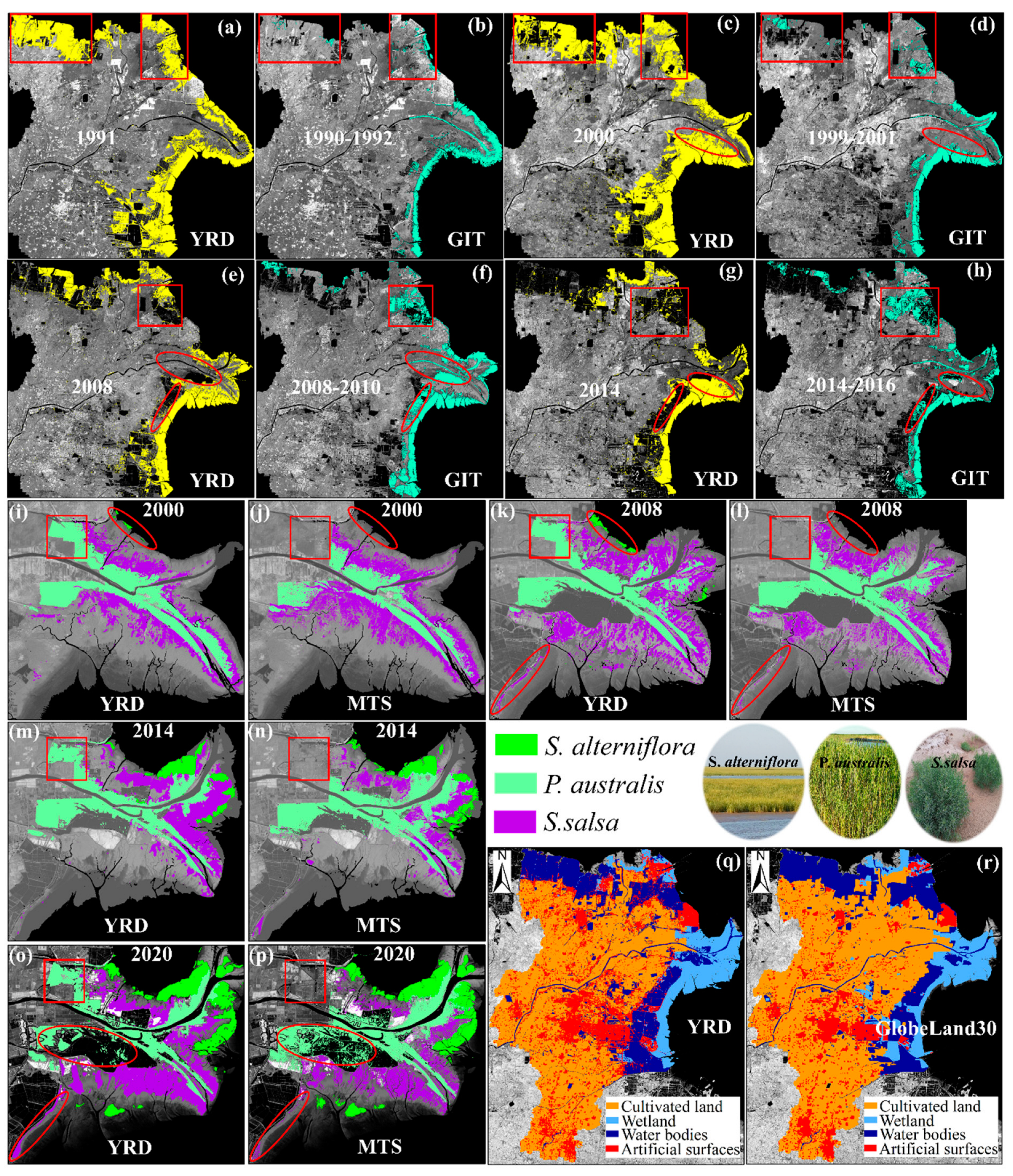
5.1. Comparison with Other Coastal Wetland Results in the YRD
5.2. The Impacts of Coastal Wetland Dynamics in the YRD Area
5.3. Advantage, Limitation and Future Study
6. Conclusions
Supplementary Materials
Author Contributions
Funding
Data Availability Statement
Conflicts of Interest
References
- Kou, W.; Dong, J.; Xiao, X.; Hernandez, A.J.; Qin, Y.; Zhang, G.; Chen, B.; Lu, N.; Doughty, R. Expansion dynamics of deciduous rubber plantations in Xishuangbanna, China during 2000–2010. GISci. Remote Sens. 2018, 55, 905–925. [Google Scholar] [CrossRef]
- Costanza, R.; D’Arge, R.; De Groot, R.; Farber, S.; Grasso, M.; Hannon, B.; Limburg, K.; Naeem, S.; O’Neill, R.V.; Paruelo, J.; et al. The value of the world’s ecosystem services and natural capital. Nature 1997, 387, 253–260. [Google Scholar] [CrossRef]
- Ericson, J.P.; Vörösmarty, C.J.; Dingman, S.L.; Ward, L.G.; Meybeck, M. Effective sea-level rise and deltas: Causes of change and human dimension implications. Glob. Planet. Chang. 2006, 50, 63–82. [Google Scholar] [CrossRef]
- Liu, Y.; Li, J.; Sun, C.; Wang, X.; Tian, P.; Chen, L.; Zhang, H.; Yang, X.; He, G. Thirty-year changes of the coastlines, wetlands, and ecosystem services in the Asia major deltas. J. Environ. Manag. 2023, 326, 116675. [Google Scholar] [CrossRef]
- Schuerch, M.; Spencer, T.; Temmerman, S.; Kirwan, M.L.; Wolff, C.; Lincke, D.; McOwen, C.J.; Pickering, M.D.; Reef, R.; Vafeidis, A.T.; et al. Author correction: Future response of global coastal wetlands to sea-level rise. Nature 2019, 569, E8. [Google Scholar] [CrossRef]
- Morris, J.T.; Sundareshwar, P.V.; Nietch, C.T.; Kjerfve, B.; Cahoon, D.R. Responses of coastal wetlands to rising sea level. Ecology 2002, 83, 2869–2877. [Google Scholar] [CrossRef]
- MacAlister, C.; Mahaxay, M. Mapping wetlands in the lower Mekong Basin for wetland resource and conservation management using Landsat ETM images and field survey data. J. Environ. Manag. 2009, 90, 2130–2137. [Google Scholar] [CrossRef] [PubMed]
- Thorne, K.; MacDonald, G.; Guntenspergen, G.; Ambrose, R.; Buffington, K.; Dugger, B.; Freeman, C.; Janousek, C.; Brown, L.; Rosencranz, J.; et al. US Pacific coastal wetland resilience and vulnerability to sea-level rise. Sci. Adv. 2018, 4, eaao3270. [Google Scholar] [CrossRef]
- Wang, B.; Zhang, K.; Liu, Q.; He, Q.; van de Koppel, J.; Teng, S.N.; Miao, X.; Liu, M.; Bertness, M.; Xu, C. Long-distance facilitation of coastal ecosystem structure and resilience. Proc. Natl. Acad. Sci. USA 2022, 119, e2123274119. [Google Scholar] [CrossRef]
- Wang, X.; Xiao, X.; Xu, X.; Zou, Z.; Chen, B.; Qin, Y.; Zhang, X.; Dong, J.; Liu, D.; Pan, L.; et al. Rebound in China’s coastal wetlands following conservation and restoration. Nat. Sustain. 2021, 4, 1076–1083. [Google Scholar] [CrossRef]
- Duan, Y.; Tian, B.; Li, X.; Liu, D.; Sengupta, D.; Wang, Y.; Peng, Y. Tracking changes in aquaculture ponds on the China coast using 30 years of landsat images. Int. J. Appl. Earth Obs. Geoinf. 2021, 102, 102383. [Google Scholar] [CrossRef]
- Mao, D.; Wang, Z.; Du, B.; Li, L.; Tian, Y.; Jia, M.; Zeng, Y.; Song, K.; Jiang, M.; Wang, Y. National wetland mapping in China: A new product resulting from object-based and hierarchical classification of Landsat 8 OLI images. ISPRS J. Photogramm. Remote Sens. 2020, 164, 11–25. [Google Scholar] [CrossRef]
- Ghosh, S.; Mishra, D.R.; Gitelson, A.A. Long-term monitoring of biophysical characteristics of tidal wetlands in the northern Gulf of Mexico—A methodological approach using MODIS. Remote Sens. Environ. 2016, 173, 39–58. [Google Scholar] [CrossRef]
- Jin, H.; Huang, C.; Lang, M.W.; Yeo, I.-Y.; Stehman, S.V. Monitoring of wetland inundation dynamics in the Delmarva Peninsula using Landsat time-series imagery from 1985 to 2011. Remote Sens. Environ. 2017, 190, 26–41. [Google Scholar] [CrossRef]
- Zhu, Z.; Wulder, M.A.; Roy, D.P.; Woodcock, C.E.; Hansen, M.C.; Radeloff, V.C.; Healey, S.P.; Schaaf, C.; Hostert, P.; Strobl, P.; et al. Benefits of the free and open Landsat data policy. Remote Sens. Environ. 2019, 224, 382–385. [Google Scholar] [CrossRef]
- Wang, X.; Xiao, X.; Zou, Z.; Hou, L.; Qin, Y.; Dong, J.; Doughty, R.B.; Chen, B.; Zhang, X.; Chen, Y.; et al. Mapping coastal wetlands of China using time series Landsat images in 2018 and Google Earth Engine. ISPRS J. Photogramm. Remote Sens. 2020, 163, 312–326. [Google Scholar] [CrossRef]
- Sun, S.; Zhang, Y.; Song, Z.; Chen, B.; Zhang, Y.; Yuan, W.; Chen, C.; Chen, W.; Ran, X.; Wang, Y. Mapping coastal wetlands of the Bohai Rim at a spatial resolution of 10 m using multiple open-access satellite data and terrain indices. Remote Sens. 2020, 12, 4114. [Google Scholar] [CrossRef]
- Sun, D.; Liu, N. Coupling spectral unmixing and multiseasonal remote sensing for temperate dryland land-use/land-cover mapping in Minqin County, China. Int. J. Remote Sens. 2015, 36, 3636–3658. [Google Scholar] [CrossRef]
- Sun, D.; Zhang, P.; Sun, Q.; Jiang, W. A dryland cover state mapping using catastrophe model in a spectral endmember space of OLI, a case study in Minqin, China. Int. J. Rem. Sens. 2019, 40, 5673–5694. [Google Scholar] [CrossRef]
- Sun, Q.; Zhang, P.; Jiao, X.; Han, W.; Sun, Y.; Sun, D. Identifying and understanding alternative states of dryland landscape: A hierarchical analysis of time series of fractional vegetation-soil nexuses in China’s Hexi Corridor. Landsc. Urban Plans. 2021, 215, 104225. [Google Scholar] [CrossRef]
- Chen, B.; Xiao, X.; Li, X.; Pan, L.; Doughty, R.; Ma, J.; Dong, J.; Qin, Y.; Zhao, B.; Wu, Z.; et al. A mangrove forest map of China in 2015: Analysis of time series Landsat 7/8 and Sentinel-1A imagery in Google Earth Engine cloud computing platform. ISPRS J. Photogramm. Remote Sens. 2017, 131, 104–120. [Google Scholar] [CrossRef]
- Wang, X.; Xiao, X.; Zou, Z.; Chen, B.; Ma, J.; Dong, J.; Doughty, R.B.; Zhong, Q.; Qin, Y.; Dai, S.; et al. Tracking annual changes of coastal tidal flats in China during 1986–2016 through analyses of Landsat images with Google Earth Engine. Remote Sens. Environ. 2018, 238, 110987. [Google Scholar] [CrossRef] [PubMed]
- Ding, X.; Shan, X.; Chen, Y.; Jin, X.; Muhammed, F.R. Dynamics of shoreline and land reclamation from 1985 to 2015 in the Bohai Sea, China. J. Geogr. Sci. 2020, 29, 2031–2046. [Google Scholar] [CrossRef]
- Ning, Z.; Li, D.; Chen, C.; Xie, C.; Chen, G.; Xie, T.; Wang, Q.; Bai, J.; Cui, B. The importance of structural and functional characteristics of tidal channels to smooth cordgrass invasion in the Yellow River Delta, China: Implications for coastal wetland management. J. Environ. Manag. 2023, 342, 118297. [Google Scholar] [CrossRef] [PubMed]
- Jiao, L.; Sun, W.; Yang, G.; Ren, G.; Liu, Y. A hierarchical classification framework of satellite multispectral/hyperspectral images for mapping coastal wetlands. Remote Sens. 2019, 11, 2238. [Google Scholar] [CrossRef]
- Liu, C.; Tao, R.; Li, W.; Zhang, M.; Sun, W.; Du, Q. Joint classification of hyperspectral and multispectral images for mapping coastal wetlands. IEEE J. Sel. Top. Appl. Earth Obs. Remote Sens. 2021, 14, 982–996. [Google Scholar] [CrossRef]
- Wang, Z.; Ke, Y.; Chen, M.; Zhou, D.; Zhu, L.; Bai, J. Mapping coastal wetlands in the Yellow River Delta, China during 2008–2019: Impacts of valid observations, harmonic regression, and critical months. Int. J. Remote Sens. 2021, 42, 7880–7906. [Google Scholar] [CrossRef]
- Zhang, C.; Gong, Z.; Qiu, H.; Zhang, Y.; Zhou, D. Mapping typical salt-marsh species in the Yellow River Delta wetland supported by temporal-spatial-spectral multidimensional features. Sci. Total Environ. 2021, 783, 147061. [Google Scholar] [CrossRef]
- GB/T 24708-2009; Wetland Classification. National Forestry and Grassland Administration: Beijing, China, 2009.
- Van der Meer, F.D.; Jia, X. Collinearity and orthogonality of endmembers in linear spectral unmixing. Int. J. Appl. Earth Obs. Geoinf. 2012, 18, 491–503. [Google Scholar] [CrossRef]
- Small, C. The Landsat ETM+ spectral mixing space. Remote Sens. Environ. 2004, 93, 1–17. [Google Scholar] [CrossRef]
- Somers, B.; Asner, G.P.; Tits, L.; Coppin, P. Endmember variability in spectral mixture analysis: A review. Remote Sens. Environ. 2011, 115, 1603–1616. [Google Scholar] [CrossRef]
- Breiman, L. Random Forests. Mach. Learn. 2001, 45, 5–32. [Google Scholar] [CrossRef]
- Palmer, D.S.; O’Boyle, N.M.; Glen, R.C.; Mitchell, J.B. Random forest models to predict aqueous solubility. J. Chem. Inf. Model. 2007, 47, 150–158. [Google Scholar] [CrossRef]
- Li, Y.; Niu, Z. Systematic method for mapping fine-resolution water cover types in China based on time series Sentinel-1 and 2 Images. Int. J. Appl. Earth Obs. Geoinf. 2022, 106, 102656. [Google Scholar] [CrossRef]
- Liu, Y.; Zhang, H.; Zhang, M.; Cui, Z.; Lei, K.; Zhang, J.; Yang, T.; Ji, P. Vietnam wetland cover map: Using hydro-periods Sentinel-2 images and Google Earth Engine to explore the mapping method of tropical wetland. Int. J. Appl. Earth Obs. Geoinf. 2022, 115, 103122. [Google Scholar] [CrossRef]
- McCarthy, M.J.; Radabaugh, K.R.; Moyer, R.P.; Muller-Karger, F.E. Enabling efficient, large-scale high-spatial resolution wetland mapping using satellites. Remote Sens. Environ. 2018, 208, 189–201. [Google Scholar] [CrossRef]
- Pontius, R.G.; Millones, M. Death to Kappa: Birth of quantity disagreement and allocation disagreement for accuracy assessment. Int. J. Remote Sens. 2011, 32, 4407–4429. [Google Scholar] [CrossRef]
- Murray, N.J.; Phinn, S.R.; DeWitt, M.; Ferrari, R.; Johnston, R.; Lyons, M.B.; Clinton, N.; Thau, D.; Fuller, R.A. The global distribution and trajectory of tidal flats. Nature 2019, 565, 222. [Google Scholar] [CrossRef]
- Ren, C.; Wang, Z.; Zhang, Y.; Zhang, B.; Chen, L.; Xi, Y.; Xiao, X.; Doughty, R.B.; Liu, M.; Jia, M.; et al. Rapid expansion of coastal aquaculture ponds in China from Landsat observations during 1984–2016. Int. J. Appl. Earth Obs. Geoinf. 2019, 82, 101902. [Google Scholar] [CrossRef]
- Yin, H.; Hu, Y.; Liu, M.; Li, C.; Chang, Y. Evolutions of 30-year spatio-temporal distribution and influencing factors of suaeda salsa in Bohai Bay, China. Remote Sens. 2022, 14, 138. [Google Scholar] [CrossRef]
- Zhang, X.; Xiao, X.; Wang, X.; Xu, X.; Chen, B.; Wang, J.; Ma, J.; Zhao, B.; Li, B. Quantifying expansion and removal of Spartina alterniflora on Chongming island, China, using time series Landsat images during 1995–2018. Remote Sens. Environ. 2020, 247, 111916. [Google Scholar] [CrossRef]
- Wu, W.; Zhi, C.; Gao, Y.; Chen, C.; Chen, Z.; Su, H.; Lu, W.; Tian, B. Increasing fragmentation and squeezing of coastal wetlands: Status, drivers, and sustainable protection from the perspective of remote sensing. Sci. Total Environ. 2022, 811, 152339. [Google Scholar] [CrossRef] [PubMed]
- Peng, J.; Liu, S.; Lu, W.; Liu, M.; Feng, S.; Cong, P. Continuous change mapping to understand wetland quantity and quality evolution and driving forces: A case study in the Liao river estuary from 1986 to 2018. Remote Sens. 2021, 13, 4900. [Google Scholar] [CrossRef]
- Yang, P.; Lai, D.Y.F.; Jin, B.; Bastviken, D.; Tan, L.; Tong, C. Dynamics of dissolved nutrients in the aquaculture shrimp ponds of the Min River estuary, China: Concentrations, fluxes and environmental loads. Sci. Total Environ. 2017, 603–604, 256–267. [Google Scholar] [CrossRef] [PubMed]
- Barbier, E.B.; Koch, E.W.; Silliman, B.R.; Hacker, S.D.; Wolanski, E.; Primavera, J.; Granek, E.F.; Polasky, S.; Aswani, S.; Cramer, L.A.; et al. Coastal ecosystem-based management with nonlinear ecological functions and values. Science 2008, 319, 321–323. [Google Scholar] [CrossRef]
- Dong, Z.; Wang, Z.; Liu, D.; Song, K.; Li, L.; Jia, M.; Ding, Z. Mapping wetland areas using landsat-derived NDVI and LSWI: A case study of west Songnen Plain, Northeast China. J. Indian Soc. Remote Sens. 2014, 42, 569–576. [Google Scholar] [CrossRef]
- Su, H.; Yao, W.; Wu, Z.; Zheng, P.; Du, Q. Kernel low-rank representation with elastic net for China coastal wetland land cover classification using GF-5 hyperspectral imagery. ISPRS J. Photogramm. Remote Sens. 2021, 171, 238–252. [Google Scholar] [CrossRef]
- Sun, W.; Liu, K.; Ren, G.; Liu, W.; Yang, G.; Meng, X.; Peng, J. A simple and effective spectral-spatial method for mapping large-scale coastal wetlands using China ZY1-02D satellite hyperspectral images. Int. J. Appl. Earth Obs. Geoinf. 2021, 104, 102572. [Google Scholar] [CrossRef]
- McCarthy, M.J.; Merton, E.J.; Muller-Karger, F.E. Improved coastal wetland mapping using very-high 2-meter spatial resolution imagery. Int. J. Appl. Earth Obs. Geoinf. 2015, 40, 11–18. [Google Scholar] [CrossRef]


| Category I | Category II | Category III | Description | Landsat-8 OLI Image Example | Field Photo Example |
|---|---|---|---|---|---|
| Natural wetlands | Wetland vegetation | S. alterniflora | S. alterniflora mainly grows in the middle and low tide areas, with its growing season from April to October. |  |  |
| P. australis | P. australis is mainly distributed in the riverbanks, with its growing season from April to October. |  |  | ||
| S. salsa | S. salsa is mainly distributed in mid-tide or high-tide area with various coverage, with its growing season of May to November. |  |  | ||
| Tidal flats | Bare flat | Bare flat is located in the mid-tide to high-tide area, with lower water content but higher soil salinization than wet tidal flat. |  |  | |
| Wet tidal flat | Wet tidal flat is located in the low tide area, has no vegetation cover, and is periodically immerged in water. |  |  | ||
| Rivers and lakes | Permanent or intermittent riverine and lacustrine wetland. |  |  | ||
| Human-made wetlands | Aquaculture | Artificial wetlands for fish/shrimp/crab/sea cucumber farming. |  |  | |
| Salt exploitation sites | Artificial wetlands for salt production. |  |  | ||
| Reservoirs | Artificial wetlands for water storage. |  |  | ||
| Paddy field | Paddy fields are mainly distributed near rivers and villages, and the single-season rice is grown in our study area. |  |  | ||
Disclaimer/Publisher’s Note: The statements, opinions and data contained in all publications are solely those of the individual author(s) and contributor(s) and not of MDPI and/or the editor(s). MDPI and/or the editor(s) disclaim responsibility for any injury to people or property resulting from any ideas, methods, instructions or products referred to in the content. |
© 2023 by the authors. Licensee MDPI, Basel, Switzerland. This article is an open access article distributed under the terms and conditions of the Creative Commons Attribution (CC BY) license (https://creativecommons.org/licenses/by/4.0/).
Share and Cite
Tan, K.; Sun, D.; Dou, W.; Wang, B.; Sun, Q.; Liu, X.; Zhang, H.; Lan, Y.; Lun, F. Mapping Coastal Wetlands and Their Dynamics in the Yellow River Delta over Last Three Decades: Based on a Spectral Endmember Space. Remote Sens. 2023, 15, 5003. https://doi.org/10.3390/rs15205003
Tan K, Sun D, Dou W, Wang B, Sun Q, Liu X, Zhang H, Lan Y, Lun F. Mapping Coastal Wetlands and Their Dynamics in the Yellow River Delta over Last Three Decades: Based on a Spectral Endmember Space. Remote Sensing. 2023; 15(20):5003. https://doi.org/10.3390/rs15205003
Chicago/Turabian StyleTan, Kun, Danfeng Sun, Wenjun Dou, Bin Wang, Qiangqiang Sun, Xiaojie Liu, Haiyan Zhang, Yang Lan, and Fei Lun. 2023. "Mapping Coastal Wetlands and Their Dynamics in the Yellow River Delta over Last Three Decades: Based on a Spectral Endmember Space" Remote Sensing 15, no. 20: 5003. https://doi.org/10.3390/rs15205003