
Multi-Label Remote Sensing Image Land Cover Classification Based on a Multi-Dimensional Attention Mechanism
1
College of Computer and Control Engineering, Northeast Forestry University, Harbin 150040, China
2
College of Computer and Information Engineering, Heilongjiang University of Science Technology, Harbin 150080, China
3
Heilongjiang Cyberspace Research Center, Harbin 150040, China
*
Author to whom correspondence should be addressed.
Remote Sens. 2023, 15(20), 4979; https://doi.org/10.3390/rs15204979
Submission received: 11 September 2023
/
Revised: 11 October 2023
/
Accepted: 13 October 2023
/
Published: 16 October 2023
(This article belongs to the Special Issue Remote Sensing and Smart Forestry II)
Abstract
:For the multi-label classification task of remote sensing images (RSIs), it is difficult to accurately extract feature information from complex land covers, and it is easy to generate redundant features by ordinary convolution extraction features. This paper proposes a multi-label classification model for multi-source RSIs that combines dense convolution and an attention mechanism. This method adds fusion channel attention and a spatial attention mechanism to each dense block module of the DenseNet, and the sigmoid activation function replaces the softmax activation function in multi-label classification. The improved model retains the main features of RSIs to the greatest extent and enhances the feature extraction of the images. The model can integrate local features, capture global dependencies, and aggregate contextual information to improve the multi-label land cover classification accuracy of RSIs. We conducted comparative experiments on the SEN12-MS and UC-Merced land cover dataset and analyzed the evaluation indicators. The experimental results show that this method effectively improves the multi-label classification accuracy of RSIs.
1. Introduction
Remote sensing image (RSI) archives have significantly increased as a result of improvements in Earth observation satellite missions. One of the most crucial tasks in remote sensing applications is the development of RSI classification systems, which aim to automatically assign class labels to each RSI. The task’s objective is to analyze the texture, space, spectrum, and other features and judge the semantic label of the target images [1]. With the deepening of research and clearer RSIs, they show more rich semantic information. Researchers are no longer satisfied with the classification of RSIs with only one label. They gradually focus on RSIs with multiple labels and apply them to image search, image auto-annotation, and scene recognition.
Monitoring and managing human-made activities requires the classification of land cover using remotely sensed terrestrial imagery collected by satellites. It is impossible to process large amounts of satellite imagery using manual methods. In recent years, computer vision multi-label classification has attracted attention. Compared with single-label images classification, multi-label images classification can better help people understand the semantic information contained in images. Multi-label learning aims to develop a function that can predict the right label set for unknown images. Each instance in this classification task has a set of class labels associated with it, and each class label is represented by a sparse binary vector. Compared with the two tasks of semantic segmentation and target detection, the advantage of multi-label image classification is that the dataset are easier to obtain. The former often requires task-heavy pixel-level labeling and bounding-box labeling, while the latter requires only image-level labeling.
Although RSI land cover classification is significant, it is often difficult to obtain satisfactory results with traditional visual classification algorithms. Because they all rely on human-designed feature extraction methods, it is more difficult to obtain high-level semantic information that is useful for image recognition. The early multi-label RSI classification methods are still implemented in multiple traditional single-label ways. It maps multi-label image classification to multiple binary single-label image classifications and obtains the final classification result by determining whether each label appears or not. Scholars proposed a series of models to predict multiple labels simultaneously, including the Conditional Random Fields (CRF) [2], the Stacked Auto Encoder (SAE) [3], and the Support Vector Machine (SVM) [4].
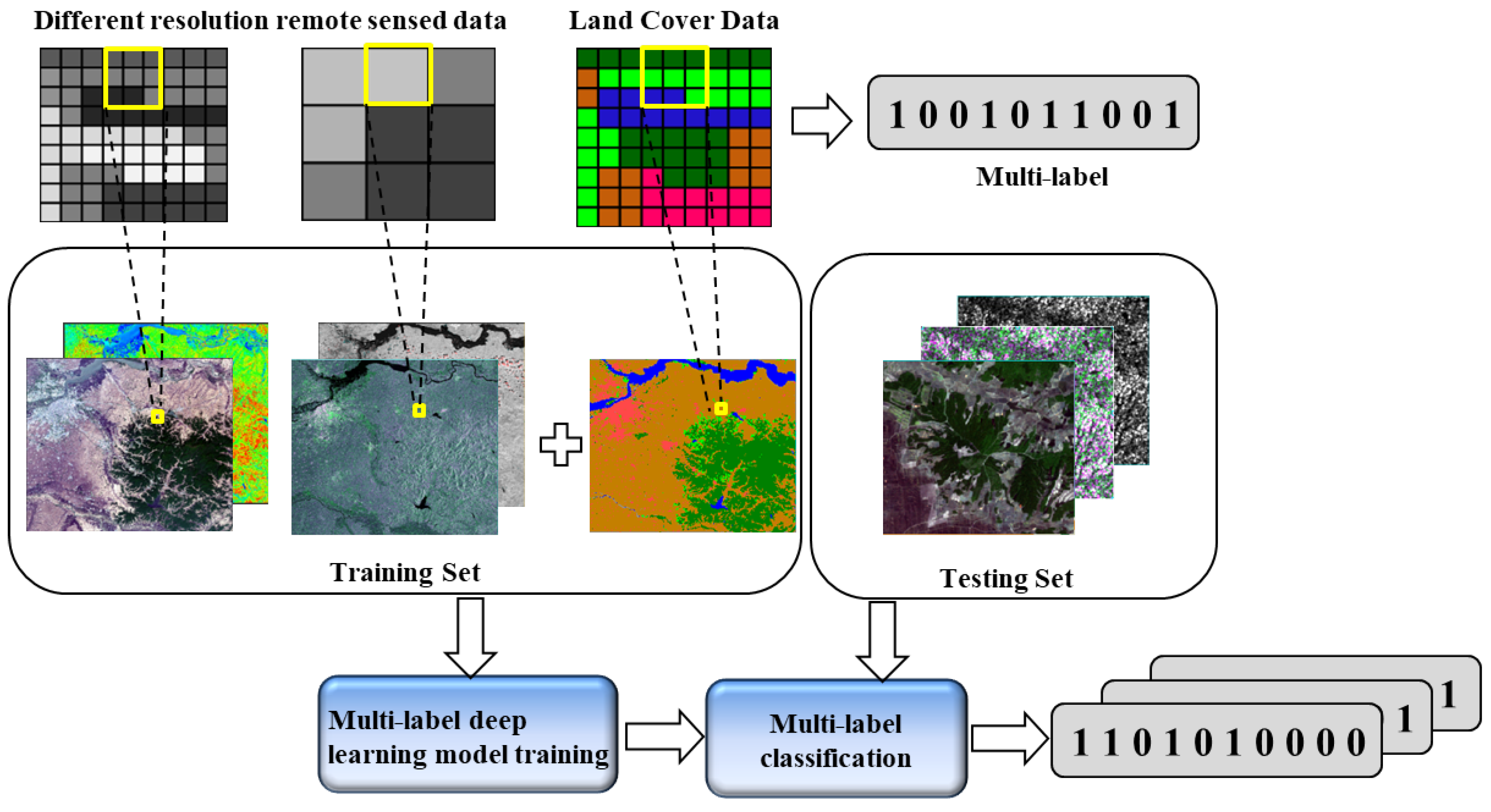
In recent years, as computer speeds have improved and image data have become more widely available, deep learning has advanced significantly and is now frequently utilized for a variety of visual identification tasks. Deep learning has powerful autonomous learning abilities and can learn to extract semantic information from images by repeating training on the training set. Therefore, deep learning models are increasingly being applied to multi-label RSI land cover classification tasks. Aiming at the problems of the large differences between classes and the high inter-class similarity of RSI, deep learning methods are not accurate enough to extract the key information of RSI and cannot significantly distinguish multiple targets. In this paper, a multi-label classification method DenseNet121-CBAM for RSIs based on dense convolution and an attention mechanism is proposed. It extracts RSI features by fusing channel attention and spatial attention, and enhances the feature extraction ability of the image. The improved network model can integrate local features, capture global dependencies, and aggregate contextual information to improve the multi-label classification accuracy of RSIs. A high-level overview of our RSI multi-label land cover classification task is depicted in Figure 1.
2. Related Work
Compared with optical images, multi-label classification in multi-source RSI is still a relatively new field with a large development space and potential. The early methods were mainly based on traditional features.
Multi-label classification techniques for RSIs based on deep features have steadily drawn researchers’ attention as deep learning technology has advanced. Zeggada et al. [5] applied deep learning algorithms to multi-labeled UAV images classification. They used a standard GoogLeNet as the backbone network of the classifier and replaced the softmax with a sigmoid function to perform multi-label classification. Koda et al. [4] and Zeggada [6] have successively used a standard neural network with an SVM or a CRF combination for multi-label classification. Khan et al. [7] proposed an optical RSI multi-label classification based on image segmentation and GCN. The algorithm uses an unsupervised image segmentation algorithm to segment the RSI into several regions and extract shape, color, texture, and SIFT features for each sub-region. A Graph structure is used to re-characterize the image, whose nodes represent the features of the region and whose edges represent the neighborhood relationships between the regions. Shendryk et al. [8] developed a CNN model that can efficiently and accurately classify the land cover advantage categories in PlantScope images. Karalas et al. [9] introduced multi-label classification applications in RSI land cover classification and produced the multi-label prediction results of the image by integrating remote sensing data with different spatial resolutions.
Attention mechanisms will help the neural network learn more effective information from an RSI. Wang et al. [10] proposed a non-local block that can be placed into neural networks, using a self-attention mechanism to model remote dependencies and incorporating global information, but the computational overhead of the network is high. The squeeze-and-excitation network (SENet) suggested by Hu et al. [11] is a model that counts the global information of an image by modeling the correlation between channels. However, SENet adjusts channel attention by weight re-tagging and does not fully utilize global contextual information. In order to give more fine-grained information and enhance the model’s capacity for learning, Woo et al. [12] created a network using the spatial and channel attention modules consecutively. The network is composed of a convolution block mechanism. In summary, a well-performing multi-label classification system requires a strong ability to learn the overall feature representation and to exploit hidden inter-class dependencies.
Many people have used deep learning networks for RSI classification research and have achieved improved results. In order to fully utilize the information included in each layer of the features and produce more specialized RSI features, Zhao et al. [13] combined dense residual blocks with multi-layer convolution features. Gao et al. [14] proposed a dual-attention perception network for remote sensing scene classification, which uses two attention modules to explore context dependence from the channel and spatial dimensions, respectively. Tong et al. [15] designed a DenseNet (CAD) CNN based on channel attention, which introduces a channel attention mechanism in the channel domain to adaptively enhance the weights of important feature channels and suppress minor feature channels. Although more deep learning methods are being used in RSI classification tasks and achieve more satisfactory results, the above methods are not accurate enough to extract key information from RSI.
3. Methodology
We present a deep learning model applicable to multi-spectral images and pol-SAR images for multi-label classification. The model is based on a densely connected CNN and incorporates a CBAM attention mechanism. Compared with ResNet, DenseNet has a smaller number of parameters, reduces vanishing-gradient, transfers features, reuses features, and reduces the number of parameters to a certain extent. Compared with the general CNN which directly depends on the high complexity features of the last layer of the model, DenseNet can comprehensively utilize the low complexity features of the shallow layers and has good anti-overfitting. Compared with SENet, CBAM improves the channel attention module and increases the spatial attention module. The model can focus on important image regions and ignore unimportant regions. Average pooling and maximum pooling are used to obtain the global statistical information of each channel, respectively, while SENet only uses average pooling. Compared with BAM [16], CBAM is not only used in bottleneck, but can be used in any intermediate convolution layer, which is a plug-and-play attention module. Therefore, we introduce the CBAM attention module in DenseNet. We believe that this model can effectively utilize more important features for the multi-label classification of RSIs. The model framework contains three parts: an image feature extraction module, an attention mechanism module, and a classifier module. We studied the performance of different deep learning networks in multi-label RSI classification through experiments. On the SEN12-MS and UC-Merced dataset, we ran tests and evaluations. Results showed that the classification performance measures outperformed other models.
3.1. Model Structure
Given an RSI, the multi-label image classification task requires the output of multiple land-cover labels embedded in the image. The multi-label classification problem of an RSI can be defined as follows: Suppose is the set of images containing M samples, is the set of labels containing N labels, and the label of is a binary vector . The n-th element in shows the presence or absence of the label . The goal of multi-label classification is to learn a mapping function F, given any image , and output the classification label , where .
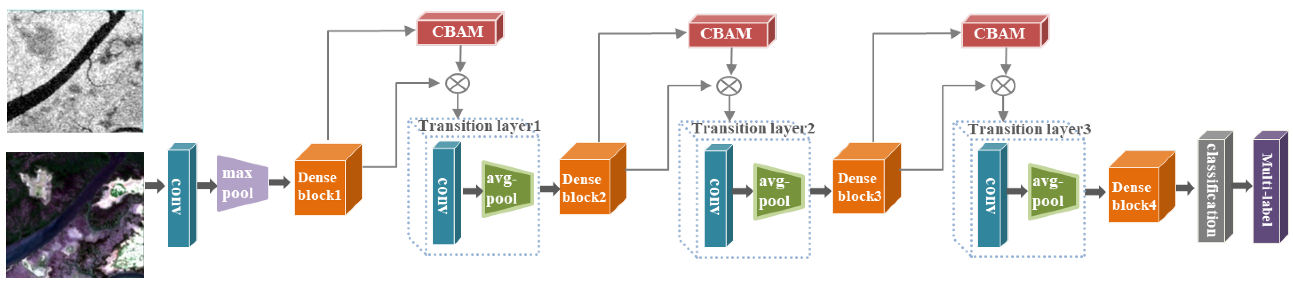
Our proposed model consists of three components: DenseNet-121, which is a model based on Dense Convolution Networks (121 represents the depth of the network), an attention module, and a classifier. Figure 2 illustrates the framework of the model.
3.2. Feature Extraction
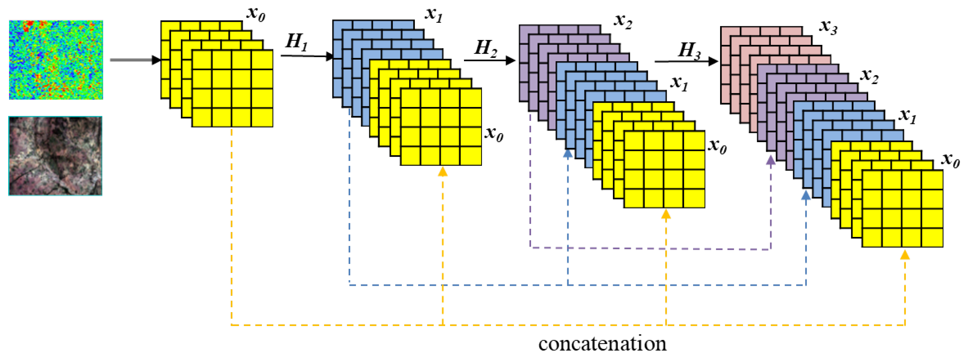
The features are extracted from pol-SAR and multi-spectral RSI using DenseNet-121 [17]. DenseNet proposes a more radical form of dense connectivity: all layers are interconnected, and every layer takes information from all earlier layers. In the channel dimension, every layer will be concatenated with every one that came before it. For each layer, the size of the feature map is the same, and it serves as the following layer’s input. For an L-layer network, Dense-Net contains connections.
is the output of the layer, where refers to the concatenation of the feature maps produced in layers . We combine ’s several inputs from Equation (1) into a single tensor. We define as a composite function of three operations: a rectified linear unit (ReLU) [18], batch normalization (BN) [19], and conv. A dense block structure with dense connections is shown in Figure 3.
and are the mean and standard deviation of mini batch , respectively; and are trainable transformation parameters (scale and shift).
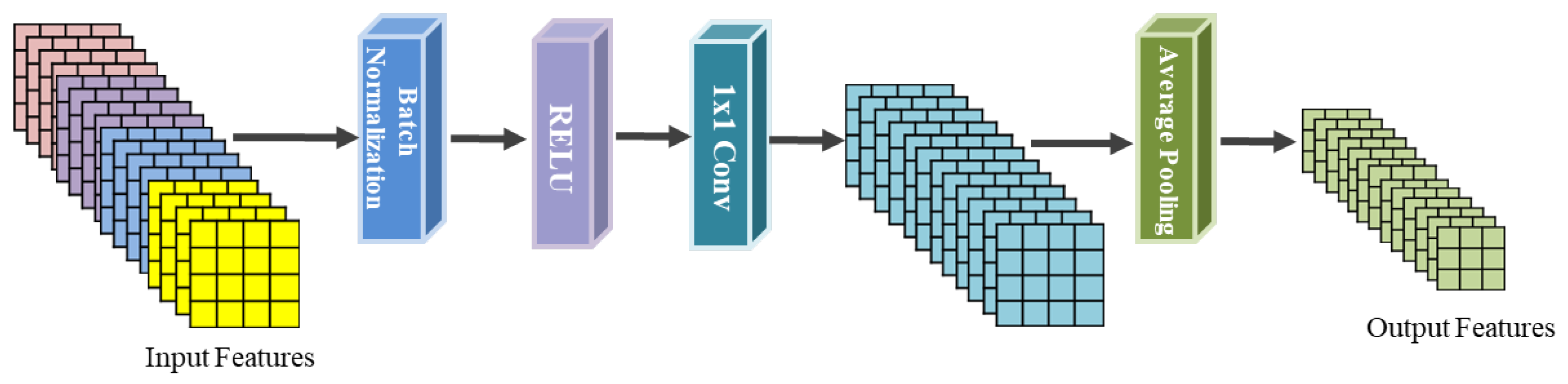
Transition layers are inserted between the dense blocks in the DenseNet network model, whose main role is to decrease the feature vector dimension extracted from the dense blocks in both the channel dimension and the spatial dimension. Its implementation structure is shown in Figure 4. Each transition layer consists of batch normalization, ReLU activation, convolution, and pooling layers. The pooling layer’s job is to lower the feature vectors in each channel in the spatial dimension.
In this paper, the backbone network is DenseNet-121. Convolution layers, dense blocks, transition layers, and an output layer make up our model structure. Each dense block has a set output feature number and is made up of an conv and a conv. To shrink the size of the feature map, each transition layer comprises an conv and a average pooling layer. Global average pooling, a full connected layer, and a sigmoid classifier are carried out at the end of the final dense block.
3.3. Attention
The concept behind computer vision’s attention mechanism is that the network can reject information from numerous features that are unimportant to the task at hand while paying attention to key feature information. It helps the neural network suppress less significant pixels or channels. DenseNet achieves dense connections between features. This method can reuse features, strengthen the transmission of features, and use features in the network more sufficiently. Moreover, this network structure can also reduce the gradient disappearance phenomenon in the process of BP to some degree. However, there are still some problems with DenseNet. Some of these features are more useful for classification, while others are not. If all these features are passed backward continuously without any difference, they cannot effectively suppress invalid information on channels and spaces. This will lead to bias in the training learning of the network, which will affect the accuracy of the multi-label RSI classification. To address this issue, we suggested an attention-CBAM technique for DenseNet.It is a simple and effective attention module for forward convolution neural networks. Given an intermediate feature map, the CBAM module will calculate the attention feature maps along two independent dimensions in turn, and then multiply the attention map with the input feature map for adaptive feature optimization.
3.3.1. CBAM Structure
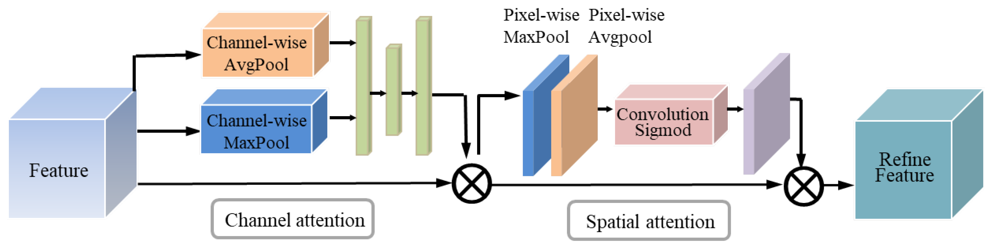
The attention module of the channel dimension (CAM) and the attention module of the spatial dimension (SAM) constitute the CBAM. The overall structure of CBAM [12] is shown in Figure 5. CBAM successively infers a one-dimensional channel attention map and a two-dimensional spatial attention map from an input feature map . Equation (3) could be used to encapsulate the attention process:
where ⨂ stands for element-by-element multiplication. The channel attention values are disseminated along the spatial dimension during multiplication, and the final refined output is the result. The two attention modules’ specifics are detailed in the following paragraphs.
3.3.2. Channel Attention Dimension Module (CAM)
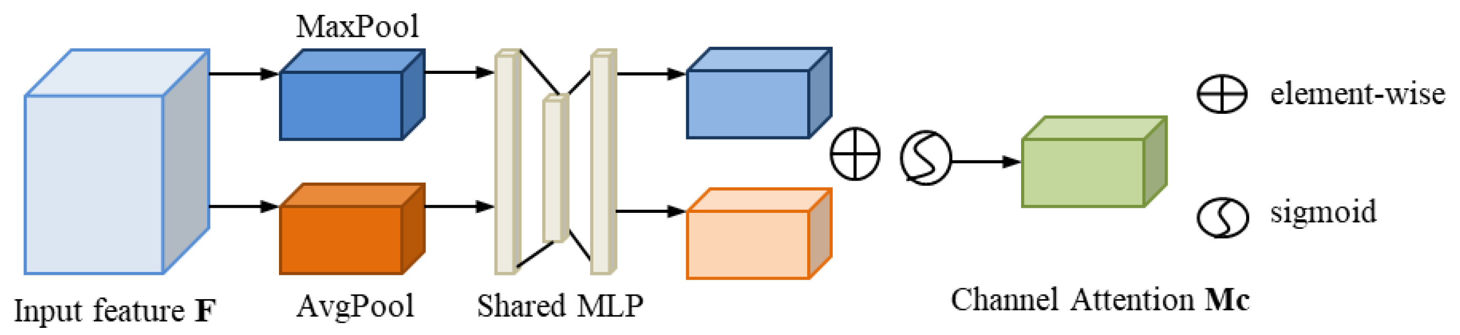
To create a channel attention map, we use the correlations between characteristics across channels. The focus of channel attention is on “what” for an input image. Figure 6 depicts the computation process of the channel dimensional attention.
The feature map is compressed in the spatial dimension by CAM to produce a 1D vector, which is then used to compute the channel dimensional attention effectively. To acquire the spatial data for the feature mapping and compress the spatial dimensions, max-pooling and average-pooling are utilized. Their outputs are then forwarded to a shared MLP with one hidden layer to produce our channel attention feature map . Equation (4) is used to compute the channel dimensional attention:
and are the MLP weights.
3.3.3. Spatial Attention Dimension Module (SAM)
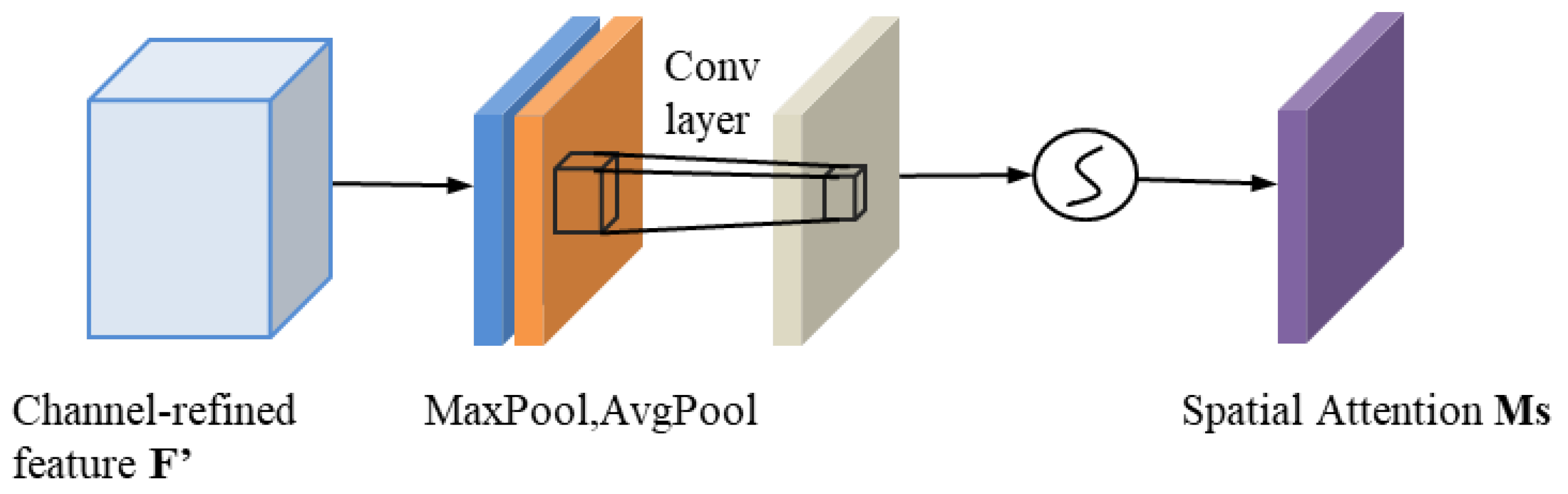
To create a spatial attention map, we use the spatial relationships between feature sets. The channel attention feature map output by CAM is used as the input for the spatial attention module. Similarly, the spatial attention module compresses the channel. In the channel dimension, it does average pooling and maximum pooling procedures. To create an effective feature descriptor, average-pooling and max-pooling procedures are applied along the channels and combined. It has been demonstrated that applying pooling techniques along the channels effectively highlights informative regions [20]. The channels are then combined into one channel after a convolution procedure. The sigmoid generates the spatial attention trait. The module’s input features and spatial features are finally multiplied to produce the final features. We describe the spatial attention module’s detailed operation below. The spatial attention module structure is shown in Figure 7.
The function of the spatial attention modules is to find the information of the target position. The spatial attention is computed as follows (5):
means a convolution operation with a filter size, and denotes the sigmoid function.
3.4. Classifier
The multi-label classifier receives the beginning and final hidden states from our model. A sigmoid activation function is used to construct a fully linked output layer with 10 probabilities. During training, binary-cross-entropy loss function iterations are used to compare the 10 probabilities in the 0–1 range to the ground-truth labels. It can solve the update delay of MSE loss function weight.In the binary classification problem, the model finally needs to predict only two cases zero or one. We predict the probability p and for each class.
stands for the label of sample i. Positive classes are 1, and negative classes are 0. stands for the probability that sample i is predicted to be a positive class.
4. Experiment
4.1. Dataset
4.1.1. SEN12MS
One of the largest RSI dataset currently accessible is SEN12MS [21], which includes Sentinel-1 dual-polarized SAR images, Sentinel-2 multi-spectral images, and MODIS-derived land cover scheme maps. A total of 180,662 patch triplets are contained in the dataset. These patches were collected all over the world throughout the year. A single “patch” corresponds to a real-world 2.56 km × 2.56 km area of land. Each patch in the dataset is an image of 256 × 256 pixels by a resolution of 10 by 10 m, meaning that each pixel represents a 10 by 10 m plot of land. As shown in Figure 8, every patch is offered as a set of 16-bit Geo-Tiff files with the following details:
Sentinel-1 SAR: C-band imaging is a feature of the Sentinel-1 mission that operates in four distinct imaging modes with varying resolutions (down to 5 m) and coverage (up to 400 km). It offers quick product delivery, dual polarization capability, and six-day return intervals at the equator. Two channels represent the dB values for sigma-no-backscatter for VV (co-polarization) and VH (cross-polarization) polarizations. The pre-processing of Sentinel-1 data includes the use of orbital files to update orbital metadata, the removal of thermal and GRD boundary noise, radiation calibration, and correction for terrain.
Sentinel-2 Multi-Spectral: Thirteen channels correspond to the 13 spectral bands: Three bands with a resolution of 60 m are associated with the atmosphere: Bands 1, 9, and 10. Bands 2, 3, 4, and 8 at a resolution of 10 m are related to the surface. The resolution of Bands 5–7, 8A, 11, and 12 is 20 m.
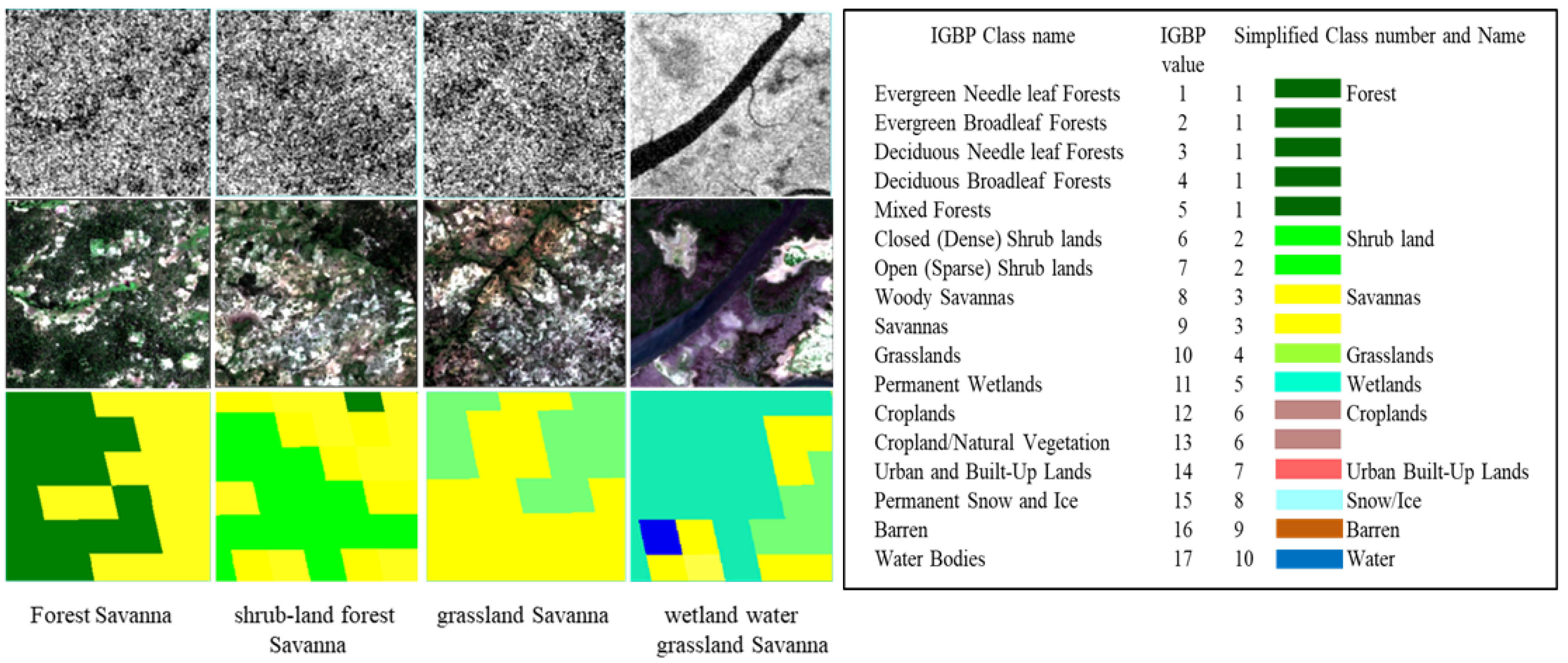
MODIS Land Cover: Using a supervised decision-tree classification algorithm, the MODIS Terra and Aqua Combined Land Cover product combines five different land cover classification schemes [22]. The principal land cover scheme identifies 17 IGBP classes, which are divided into 11 classes of naturally occurring vegetation, 3 classes of vegetation that has undergone human influence, and 3 classes of uninhabited land. We selected four land cover schemes as dataset labels, and the four channels of the label images correspond to IGBP, Land Cover Classification System (LCCS) land cover, LCCS land use, and LCCS surface water layer individually. The data was generated from 2016 data and re-sampled to a pixel resolution of 10 m.
There are four distinct MODIS land cover labeling systems in the SEN12MS dataset. The IGBP scheme was chosen as the classification standard for conversion to multi-label classification dataset among these schemes. This is because the IGBP scheme comprises common categories with a medium level of semantic granularity, including natural and urban habitats. Other LCCS cover classification techniques, in comparison, are uncommon and put an excessive amount of emphasis on unrelated subjects of interest such as land use or surface hydrology. In order to provide comparability with other land cover schemes and partially alleviate the classification balance of SEN12MS, the initial 17 classes of IGBP proposed by Yokoya [23] were reduced to 10 simplified IGBP schemes. Our experiment used the simple 10 IGBP classes as classification training and testing classes.
Probability vectors are used to depict land cover scene classifications based on the entire IGBP in the dataset. The probability vector displays the patch’s overall coverage for each class. In our experiment, we read the probability labels in the original IGBP scheme and converted them into a multi-label, simplified IGBP land cover scheme.
4.1.2. UC-Merced
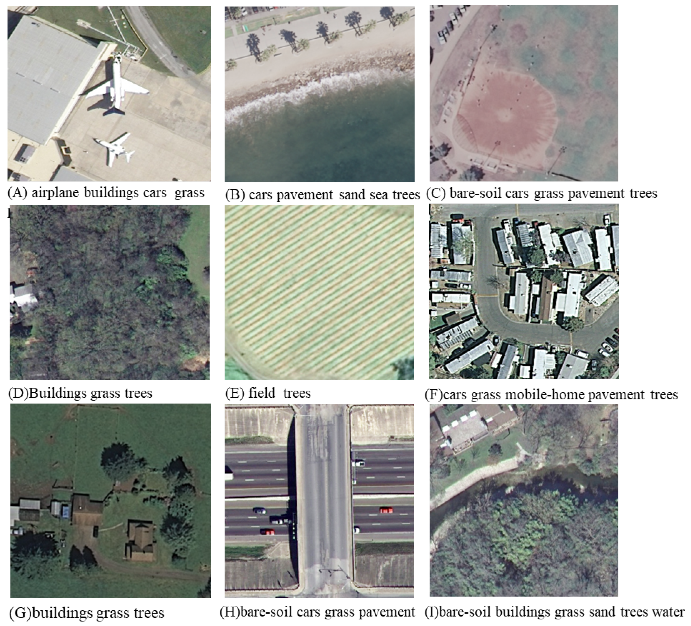
The UC-Merced Dataset [24,25] is a ground truth RSI that has been hand-labeled. Each image was downloaded from the National Map of the U.S.G.S. in the R.G.B. color space. The UC-Merced multi-label database is the first database applied to the multi-label classification of RSIs published in 2018. The database contains a total of 2100 RSIs from the UC-Merced single-label scene database with a resolution of 0.3 m. Each of these images is given a category label for the different objects contained in it. There are 17 label categories in the dataset: airplane, bare-soil, car, chaparral, pavement, court, building, tree, dock, mobile-home, sand, ship, storage tank, water, grass, sea, and field. As shown in Figure 9.
4.2. Training Details
The experiment runs on the linux operating system. The deep learning framework is Pytorch 1.9.0 and Python 3.7. The CPU is an Intel (R) Xeon (R) Sliver 4208 with 8 cores and 2.1 GHz. The GPU is an NVIDIA Tesla V100 and CUDA version 12.0. The Python library files need rasterio, scikit-learn, tensorboardX, tqdm, etc. According to the mathematical properties of the ADAM [26] optimizer, if the learning rate is too large, the loss function will fluctuate such that it is difficult to converge to the optimal value; on the contrary, if the learning rate is too small, the optimization rate will be low and cannot converge for a long time. Therefore, we set the learning rate of ADAM to be 0.001, the decay rate to be , and the batch size to be 64. We use Sentinel-1 dual-pol SAR data with two channels and Sentinel-2 multi-Spectral with 10 channels as input. The mean and standard deviation of Sentinel-1 SAR and Sentinel-2 multi-spectral images were calculated for normalization. Our model training process is shown in Algorithm 1.
| Algorithm 1: The training process of the proposed model. |
 |
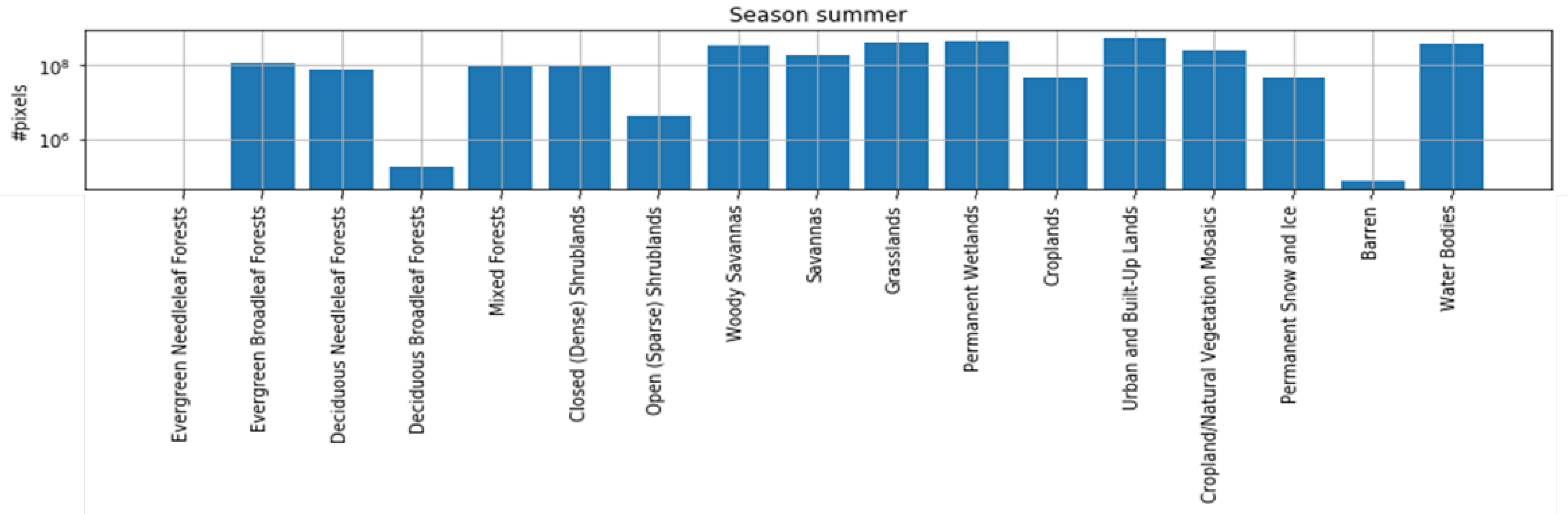
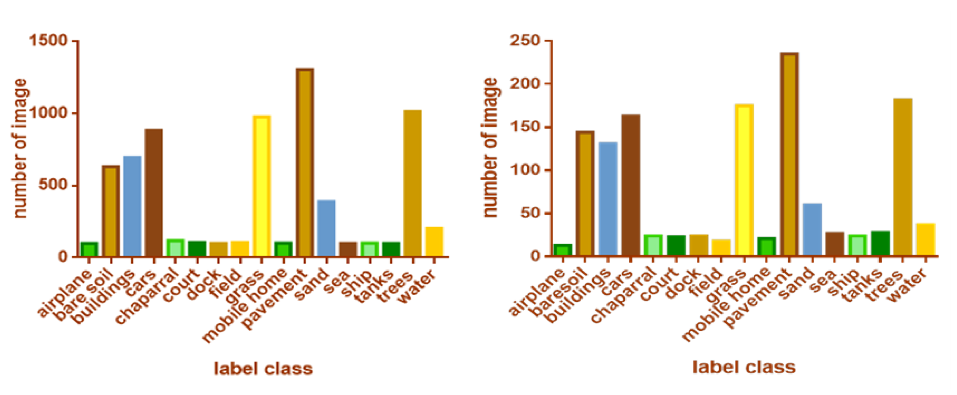
The class distribution in the SEN12MS dataset is shown in Figure 10. The UC-Merced total images number and test images number is shown in Figure 11. It is important to note that although the number of barren samples is lower in comparison to the other classes.
Generally, 0.5 is used as the classification threshold, but 0.5 is not suitable for all land cover. A threshold value is used to convert IGBP probability labels to multi-hot labels. The mean/std for normalization will not be accurate if the threshold is larger than 0.22. Therefore, the threshold parameter is set to 0.1.The training-set images are pre-processed to a resolution of and require 2k initial convolution layers of with a step size of 2 and a maximum pooling layer with a step size of 2 before entering the first dense block. A convolution layer is added after each convolution layer to increase computational efficiency and reduce the amount of input feature maps. In order to preserve the size of the feature maps, the convolution kernel of the convolution layer uses zero padding in the dense blocks. A fully connected layer and an global average pooling layer constitute the last classification layer. A sigmoid activation function is lastly used to complete the multi-label classification task for RSIs. It is required that the target be in the form of a one-hot label. The detailed configuration of the parameters and output of our model is shown in Table 1. We chose summer scenes including 45,753 patch triples as the training set for our model.
We trained the model on the UC-Merced dataset by an Adam optimizer with a weight decay of over 30 epochs, a learning rate of that is reduced after 8 epochs, and a batch size of 32. We used the ReduceLROnPlateau function to optimally reduce the learning rate during the training process. We made a number of adjustments to broaden the variety of photos used for data augmentation in order to increase adaptability and avoid overfitting Unlike natural images in ImageNet, RSIs can retain semantic features after flipping and rotating, so we applied both horizontal flipping and vertical flipping. Each image was rotated randomly by no more than 45 degrees. The width shift-range and height shift-range equal 0.2. The model obtains loss results on the validation set at the end of each epoch, and training stops if the loss is found to rise on the validation set. The model takes the weights after stopping as the final parameters.
4.3. Evaluation
The performance evaluation of multi-label classification models requires an analysis of multiple indicators, not just the number of correctly predicted labels, so a more complicated analysis process is needed compared with the single-label case.
Each sample can be associated with many labels simultaneously since the performance evaluation of multi-label classification is significantly more complicated than that of conventional single-label classification. There have been many evaluation indicators suggested for multi-label learning. These indicators can be broadly categorized as example-based metrics and label-based metrics. The method’s main idea is to split the multi-label learning classification problem into q distinct binary classification problems, each of which resolves to a class label. The indicators for evaluating performance classification can be calculated based on the following methods: The importance of each sample in the test set is made equal (sample average), each class’s importance is made equal (macro average), and the entire test set is compared to the ground reference, regardless of the relative value of each sample or class (micro-average method).
In this paper, the macro scores and micro scores are used to evaluate the experimental results, using the following equations [27]:
These involve True Positive (), True Negative (), False Positive (), and False Negative () test samples. stands for the symmetric difference between two sets. According to the above definitions, naturally holds for the j-th class. The misclassification of samples on a single label is investigated using Hamming Loss [28]. The percentage of relevant labels that do not appear in the anticipated label set and irrelevant labels is calculated. For Hamming Loss, a smaller value indicates a superior classification result from the model.
The majority of binary classification metrics can be calculated based on the values provided above. Let represent some specific binary classification metrics. The following formulas (Equations (13) and (14)) contain metrics for label-based classification. Conceptually, labels and instances are given “equal weights” in macro- and micro-averaging, respectively. The higher values obtained indicates improved model classification performance.
Macro-averaging
Micro-averaging
To understand how the system performs generally across the dataset, we can utilize the macro-average metrics for analysis. Because all classifications are equally important, the overall results are greatly affected by small categories. The highest scores were obtained from our model and are listed in Table 2. This average should not be used to make any specific decisions. On the other hand, when the categories in a dataset are uneven, the micro average can be a useful statistic. Table 3 lists micro-averaging scores for the different CNN models in the SEN12-MS dataset.
In the experiment, we evaluated the suggested model against the following models: (1) deep convolution networks (VGG19 [29]), (2) Deep Residual Nets (ResNet50) [30], and (3) Densely Connected Convolution Networks (DenseNet-121). The experimental findings demonstrate that the classification effect improves as learning model depth increases. The classification scores improve when model depth is increased, demonstrating that multi-label classification benefits from model depth. By using CBAM attention and the Dense Connect Network as the feature extractor, our model outperformed the other models, as shown by the indicators in Table 2 and Table 3.
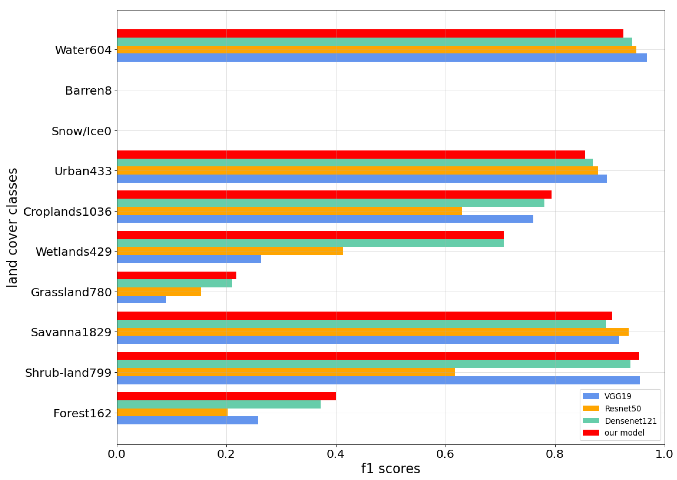
Since we transform IGBP probability vector dense labels into simple scene labels, the number of barren labels is insufficient. In the multi-label test dataset, only eight patches support barren labels. This makes the test results for the barren class inaccurate. The shrub-land, savanna, and water areas obtained higher F1 scores, indicating that the model was highly significant in predicting dense label classes. Figure 12 shows the F1 score distribution for each label, which is similar to the label frequency distribution displayed in Figure 10. This is appropriate given that the model can learn more category features and produce better classification outcomes with more data. Visually confused labels such as barren, forest, and grassland are present in different samples, so their F1 scores are significantly lower due to a severe lack of fitting.
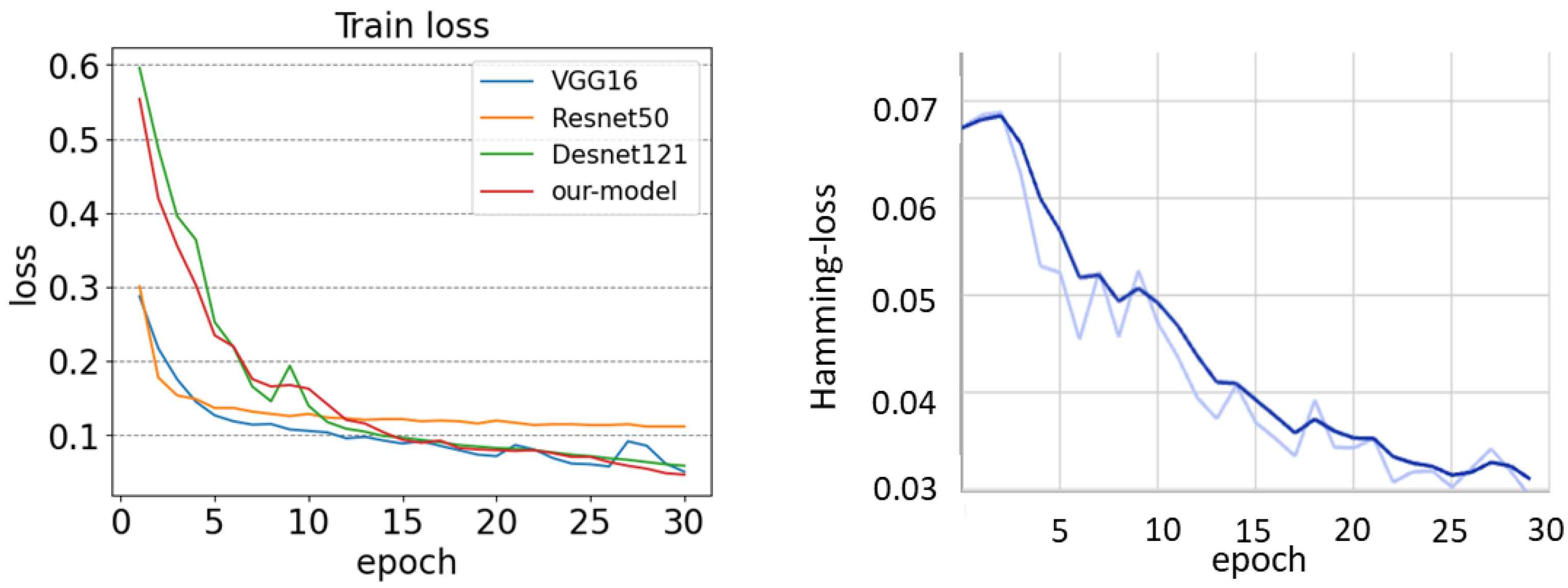
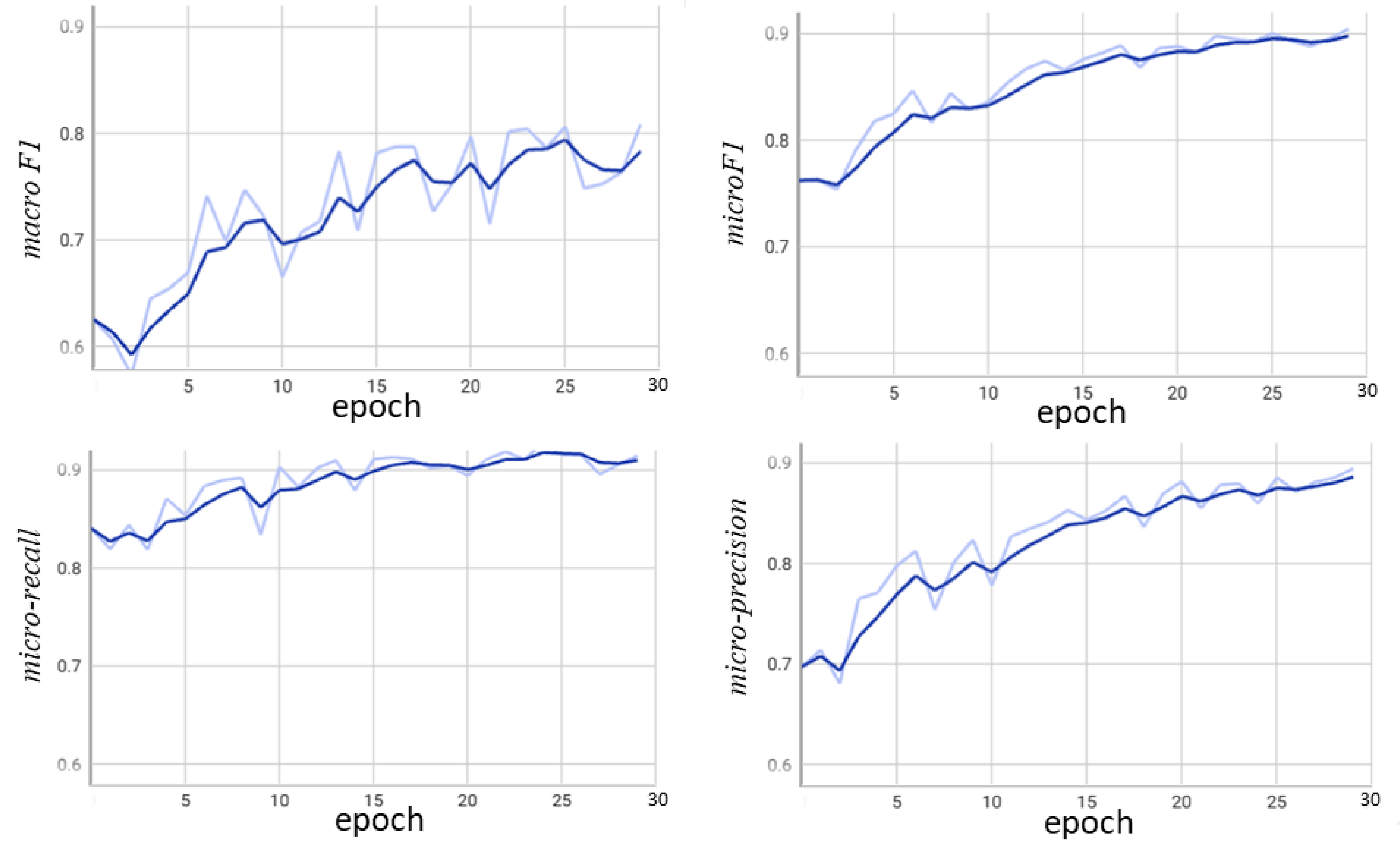
Figure 13 shows the loss curve graph of models during 30 training epochs and the hamming loss curves in the validation set during the validation epochs. As the training epoch increases, the loss value decreases, and the F1 score, precision, and recall gradually increase during the validation period, indicating that our model has not suffered from over-fitting. The validation set index process with the Tensorboard tool is shown in Figure 14.
In the experiment on the UC-Merced dataset, we selected three deep learning CNNs (VGG16, InceptionV3 [31], and Resnet50) for pre-training on the ImageNet dataset and applied the training parameters to the multi-label UC-Merced dataset for fine-tuning. The experiment micro-averaging results on UC-Merced are shown in Table 4.
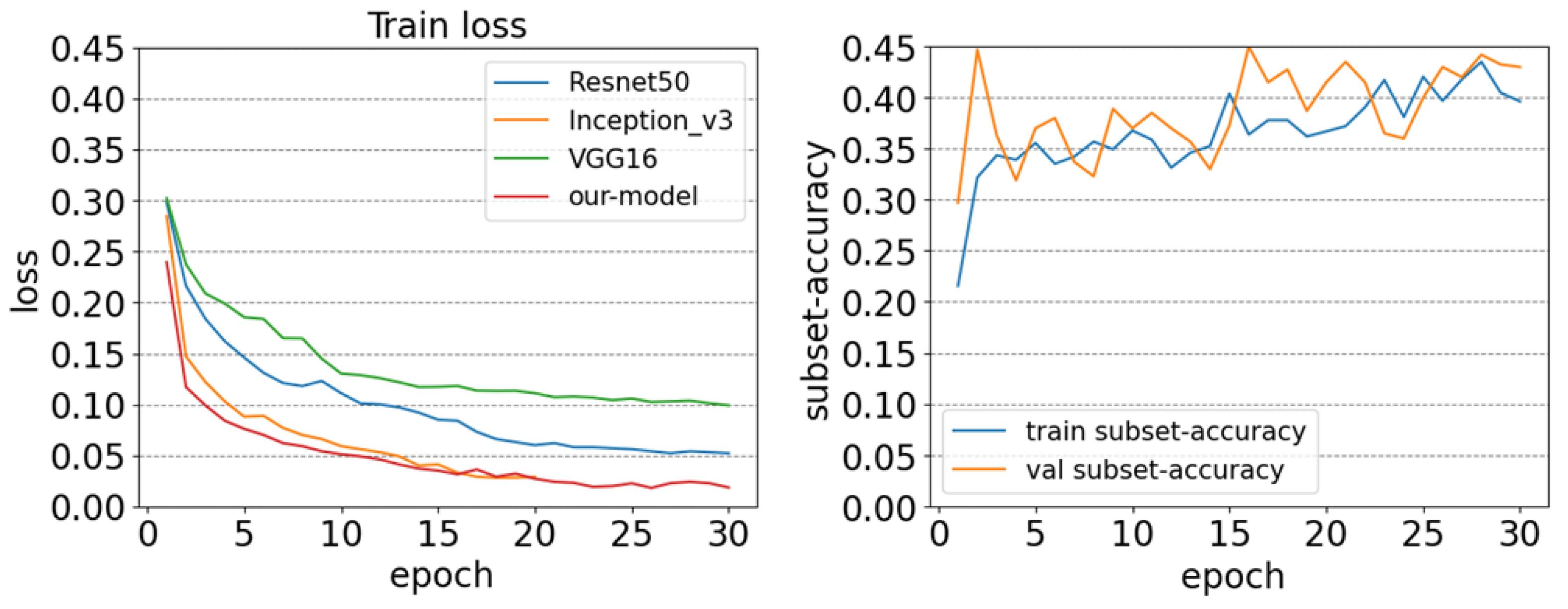
We trained the above models based on the UC-Merced multi-label dataset for iterations and recorded the subset-accuracy values and loss values of the models for each epoch. The training set is used for cross validation, parameter tuning, and feature selection, and the testing set is usedfor measuring the accuracy of model. Experimentally, each model reached the state of convergence after 30 epochs of training. Figure 15 (left) shows the training result curves of each model on the UC-Merced multi-label dataset. In the training process, the early stopping [32] mechanism was used to avoid overfitting. Inception V3 ended training early at the 20th epoch. With regard to convergence stability and speed, our model outperformed the other three models in both loss values and F1 values. Our model provides a good training starting point for weight initialization.
With the increase in training epochs in SEN12-MS, the curves of the other three CNN models fluctuate greatly, indicating that the fitting of these models is not inferior to ours. However, the CBAM-DenseNet model we proposed has no obvious fluctuation. In addition, in the 25th training iteration of UC-Merced, the DenseNet-CBAM model has the lowest loss value and is more stable than other CNN models. From the overall results of the two dataset, it can be found that the proposed model is superior to the other four CNN models in macro-average and micro-average indicators. Although the macro-Recall indicator is slightly lower than that of DenseNet121, the comprehensive performance can still show the effectiveness of the proposed method. This shows that the generalization performance of the model is high.
The experimental results compared with other CNN models on the UC-Merced dataset are shown in Table 4. The micro-F1 and micro-Recall of our model are higher than those of the other three methods, but the micro-precision value is lower than that of the VGG16 and InceptionV3 models. Compared with micro-precision, micro-F1 can better reflect the comprehensive performance of the models. In general, on the UC-Merced dataset, our model’s classification performance measures outperform those of the other three models.
The training process and test results of the two datasets show that the deeper the network is, the better the results are on the large-scale dataset of SEN12-MS. However, on the smaller UC-Merced dataset, the deepening of the network layer has no significant effect on the final result. It is proven that the current data-driven method represented by deep neural networks requires ultra-large-scale labeled data to meet the needs of deep network model training. However, UC-Merced dataset do not exceed 3000 annotated images. When training a deep network with tens of millions of model parameters, even if training samples are expanded by data augmentation during the training period, the overfitting of model parameters still easily occurs, such that a deep network model with high performance cannot be effectively trained.
4.4. Discussion
We carried out two qualitative studies of the proposed model, including a case study and a label-specific feature visualization, in order to better illuminate its efficacy [33]. The case study shows the prediction results of some images of the proposed model on the SEN12-MS and UC-Merced datasets, as shown in Table 5. Furthermore, the feature heat map visualization of a specific label reveals a specific image region corresponding to the label, as shown in Figure 16.
To further verify the real performance of our model, three representative image examples were selected from the SEN12-MS and UC-Merced datasets to show their classification results. According to the different densities of the labels, the images with dense labels and sparse labels were selected, respectively. For example, the grassland label was not predicted in image (a), because most of the grassland has become bare-soil in the multi-spectral visual image, resulting in reduced grassland features, so the label was not recognized. There are savanna and forest labels in image (c), but our model could correctly identify the urban/built-up area in the image. The content of image (e) is complex, with up to six ground object labels: cars, buildings, court, pavement, grass, and trees. Our model correctly identifies all the above labels in the multi-label image classification results. Image (f) contains seven different labels: cars, bare-soil, buildings, grass, trees, court, and pavement. Only grass is not accurately predicted by the model. With regard to RSIs with few labels, the model can also classify correctly.
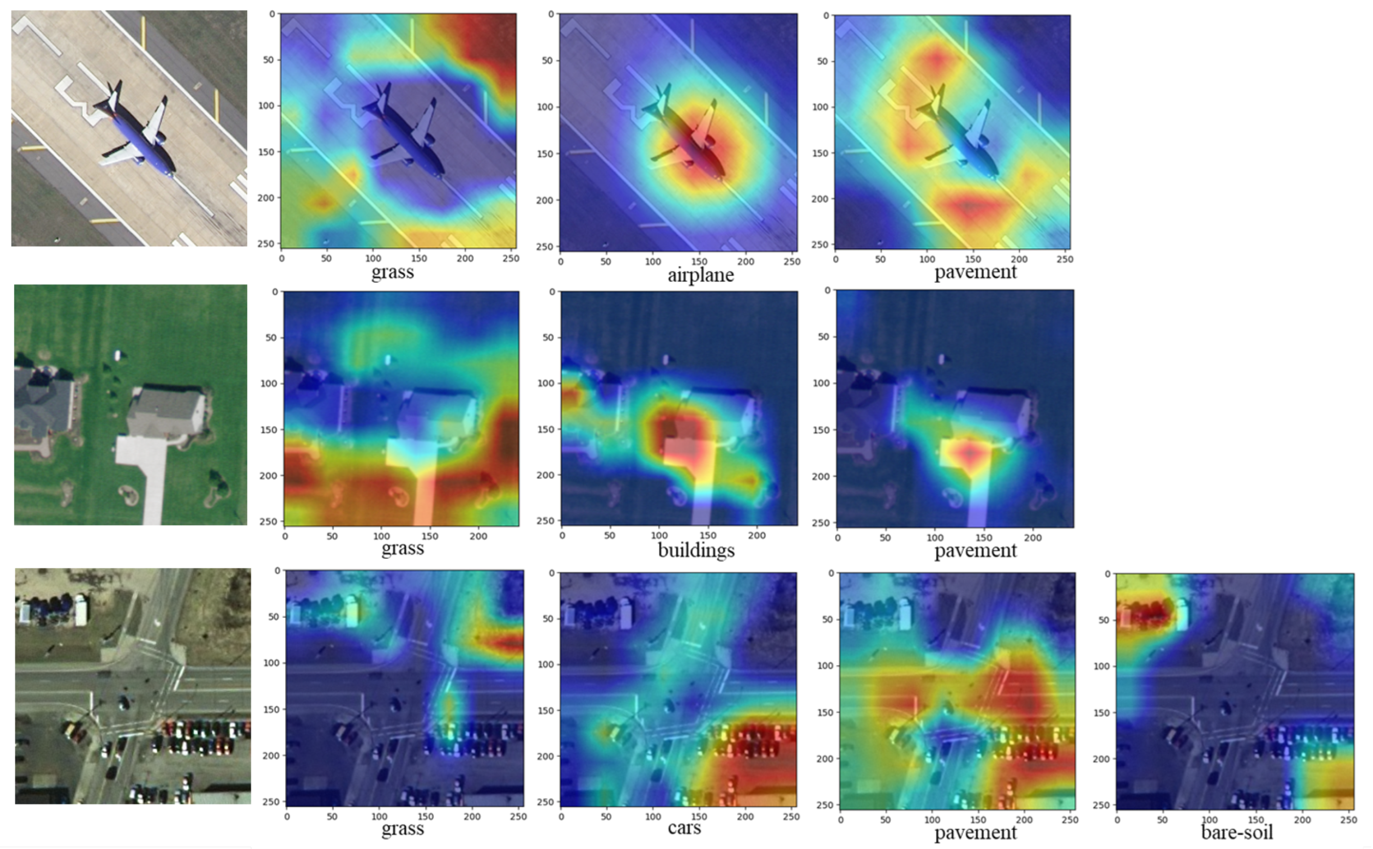
In order to further investigate the efficacy of the proposed model for multi-label interpretation of RSIs, label-specific feature heat maps of some image examples in the UC-Merced dataset were visualized by the Grad-cam [34] tool. Figure 16 displays the outcomes of qualitative studies that demonstrate the visual interpretation process of the model for RSIs. It lists the regional activation of the heat maps of the three images under different labels. Among them, the red part indicates that the region has a high degree of correspondence with the label, and is activated strongly. The blue part indicates that the region is less associated with the label and is activated weakly. The results show that the image region with the most semantic information associated with the labels is focused and highlighted in the heat map. At the same time, image regions with less semantic information associated with labels are less activated or focused.
Although our proposed method has made progress in multi-label RSI classification, there are still problems. The potential links between labels are completely ignored by binary correlations. Label correlation is the co-occurrence dependence of different labels in the same RSI. Moreover, each class label’s binary classifier may experience category imbalance. This will mean that a small amount of data cannot be well trained. In our upcoming work, we’ll strive to use label correlation to boost the multi-label RSI’s classification performance. In addition, a overly high number of parameters in a deep learning model is still the main problem that limits the interpretation ability of deep learning models. Therefore, we will try to improve the model structure to solve the feature unknowns of deep learning.
5. Conclusions
Due to the large difference in images in the same category, the high similarity of images in different categories, and the complex background of remote sensing scene images, the performance of a CNN for land cover classification is weakened. This study proposes a model based on an improved dense connection network. Compared with other CNNs, our proposed model can better notice target areas in different remote sensing scenarios, so as to perform multi-label classification more accurately. The model introduces the CBAM multi-dimensional attention module into DenseNet121 to reduce redundant features, increase useful information, retain the main features of RSI, and improve feature extraction. Experiment’s results indicate that the improved model performs well, and subset accuracy on the SEN12-MS dataset is 1.2% higher than that on DenseNet121. The Micro-F1 on the UC Merced dataset is 0.92. Because there are many and small land cover targets in high-resolution RSIs, the amount of calculation is inevitably increased when the attention mechanism and multiple convolutions are introduced. Designing a model that can be processed in real time and improving the overall running speed will be the focus of future research. In the actual RSI classification tasks, the complex background information of RSIs has a great influence on the effective extraction of image features. Therefore, further research on effective feature learning based on noise data is another important component of future research on multi-label RSI classification.
Author Contributions
Conceptualization, H.Y.; methodology, H.Y. and W.J.; resources, J.G.; writing—original draft preparation, H.Y.; writing—review and editing, H.Y., W.J., J.G.; validation, H.Y. All authors have read and agreed to the published version of the manuscript.
Funding
This research was funded by National Natural Science Foundation of China grant number 32171777 and Natural Science Foundation of Heilongjiang for Distinguished Young Scientists grant number JQ2023F002.
Data Availability Statement
Not applicable.
Conflicts of Interest
The authors declare no conflict of interest.
References
- Sumbul, G.; Demİr, B. A deep multi-attention driven approach for multi-label remote sensing image classification. IEEE Access 2020, 8, 95934–95946. [Google Scholar] [CrossRef]
- Zhang, T.; Yan, W.; Li, J.; Chen, J. Multiclass labeling of very high-resolution remote sensing imagery by enforcing nonlocal shared constraints in multilevel conditional random fields model. IEEE J. Sel. Top. Appl. Earth Obs. Remote Sens. 2016, 9, 2854–2867. [Google Scholar] [CrossRef]
- Law, A.; Ghosh, A. Multi-label classification using a cascade of stacked autoencoder and extreme learning machines. Neurocomputing 2019, 358, 222–234. [Google Scholar] [CrossRef]
- Koda, S.; Zeggada, A.; Melgani, F.; Nishii, R. Spatial and structured SVM for multilabel image classification. IEEE Trans. Geosci. Remote. Sens. 2018, 56, 5948–5960. [Google Scholar] [CrossRef]
- Zeggada, A.; Melgani, F.; Bazi, Y. A deep learning approach to UAV image multilabeling. IEEE Geosci. Remote Sens. Lett. 2017, 14, 694–698. [Google Scholar] [CrossRef]
- Zeggada, A.; Benbraika, S.; Melgani, F.; Mokhtari, Z. Multilabel conditional random field classification for UAV images. IEEE Geosci. Remote. Sens. Lett. 2018, 15, 399–403. [Google Scholar] [CrossRef]
- Khan, N.; Chaudhuri, U.; Banerjee, B.; Chaudhuri, S. Graph convolutional network for multi-label VHR remote sensing scene recognition. Neurocomputing 2019, 357, 36–46. [Google Scholar] [CrossRef]
- Shendryk, I.; Rist, Y.; Lucas, R.; Thorburn, P.; Ticehurst, C. Deep learning-a new approach for multi-label scene classification in planetscope and sentinel-2 imagery. In Proceedings of the IGARSS 2018-2018 IEEE International Geoscience and Remote Sensing Symposium, Valencia, Spain, 22–27 July 2018; pp. 1116–1119. [Google Scholar]
- Karalas, K.; Tsagkatakis, G.; Zervakis, M.; Tsakalides, P. Land classification using remotely sensed data: Going multilabel. IEEE Trans. Geosci. Remote Sens. 2016, 54, 3548–3563. [Google Scholar] [CrossRef]
- Wang, X.; Girshick, R.; Gupta, A.; He, K. Non-local neural networks. In Proceedings of the IEEE Conference on Computer Vision and Pattern Recognition, Salt Lake City, UT, USA, 18–23 June 2018; pp. 7794–7803. [Google Scholar]
- Hu, J.; Shen, L.; Sun, G. Squeeze-and-excitation networks. In Proceedings of the IEEE Conference on Computer Vision and Pattern Recognition, Salt Lake City, UT, USA, 18–23 June 2018; pp. 7132–7141. [Google Scholar]
- Woo, S.; Park, J.; Lee, J.Y.; Kweon, I.S. Cbam: Convolutional block attention module. In Proceedings of the European Conference on Computer Vision (ECCV), Munich, Germany, 8–14 September 2018; pp. 3–19. [Google Scholar]
- Zhao, X.; Zhang, J.; Tian, J.; Zhuo, L.; Zhang, J. Residual dense network based on channel-spatial attention for the scene classification of a high-resolution remote sensing image. Remote Sens. 2020, 12, 1887. [Google Scholar] [CrossRef]
- Gao, Y.; Shi, J.; Li, J.; Wang, R. Remote sensing scene classification with dual attention-aware network. In Proceedings of the 2020 IEEE 5th International Conference on Image, Vision and Computing (ICIVC), Beijing, China, 10–12 July 2020; pp. 171–175. [Google Scholar]
- Tong, W.; Chen, W.; Han, W.; Li, X.; Wang, L. Channel-attention-based DenseNet network for remote sensing image scene classification. IEEE J. Sel. Top. Appl. Earth Obs. Remote Sens. 2020, 13, 4121–4132. [Google Scholar] [CrossRef]
- Park, J.; Woo, S.; Lee, J.Y.; Kweon, I.S. Bam: Bottleneck attention module. arXiv 2018, arXiv:1807.06514. [Google Scholar]
- Huang, G.; Liu, Z.; Van Der Maaten, L.; Weinberger, K.Q. Densely connected convolutional networks. In Proceedings of the IEEE Conference on Computer Vision and Pattern Recognition, Honolulu, HI, USA, 21–26 July 2017; pp. 4700–4708. [Google Scholar]
- Glorot, X.; Bordes, A.; Bengio, Y. Deep sparse rectifier neural networks. In Proceedings of the Fourteenth International Conference on Artificial Intelligence and Statistics. JMLR Workshop and Conference Proceedings, Fort Lauderdale, FL, USA, 11–13 April 2011; pp. 315–323. [Google Scholar]
- Ioffe S, S.C. Batch normalization: Accelerating deep network training by reducing internal covariate shift. In Proceedings of the International Conference on Machine Learning.pmlr, Lille, France, 6–11 July 2015; pp. 448–456. [Google Scholar]
- Zagoruyko, S.; Komodakis, N. Paying more attention to attention: Improving the performance of convolutional neural networks via attention transfer. arXiv 2016, arXiv:1612.03928. [Google Scholar]
- Schmitt, M.; Hughes, L.H.; Qiu, C.; Zhu, X.X. SEN12MS–A Curated Dataset of Georeferenced Multi-Spectral Sentinel-1/2 Imagery for Deep Learning and Data Fusion. arXiv 2019, arXiv:1906.07789. [Google Scholar] [CrossRef]
- Sulla-Menashe, D.; Gray, J.M.; Abercrombie, S.P.; Friedl, M.A. Hierarchical mapping of annual global land cover 2001 to present: The MODIS Collection 6 Land Cover product. Remote Sens. Environ. 2019, 222, 183–194. [Google Scholar] [CrossRef]
- Yokoya, N.; Ghamisi, P.; Xia, J.; Sukhanov, S.; Heremans, R.; Tankoyeu, I.; Bechtel, B.; Le Saux, B.; Moser, G.; Tuia, D. Open data for global multimodal land use classification: Outcome of the 2017 IEEE GRSS data fusion contest. IEEE J. Sel. Top. Appl. Earth Obs. Remote Sens. 2018, 11, 1363–1377. [Google Scholar] [CrossRef]
- Yang, Y.; Newsam, S. Bag-of-visual-words and spatial extensions for land-use classification. In Proceedings of the 18th SIGSPATIAL International Conference on Advances in Geographic Information Systems, San Jose, CA, USA, 2–5 November 2010; pp. 270–279. [Google Scholar]
- Chaudhuri, B.; Demir, B.; Chaudhuri, S.; Bruzzone, L. Multilabel remote sensing image retrieval using a semisupervised graph-theoretic method. IEEE Trans. Geosci. Remote Sens. 2017, 56, 1144–1158. [Google Scholar] [CrossRef]
- Kingma, D.P.; Ba, J. Adam: A method for stochastic optimization. arXiv 2014, arXiv:1412.6980. [Google Scholar]
- Zhang, M.L.; Zhou, Z.H. A review on multi-label learning algorithms. IEEE Trans. Knowl. Data Eng. 2013, 26, 1819–1837. [Google Scholar] [CrossRef]
- Dembczyński, K.; Waegeman, W.; Cheng, W.; Hüllermeier, E. Regret analysis for performance metrics in multi-label classification: The case of hamming and subset zero-one loss. In Proceedings of the Machine Learning and Knowledge Discovery in Databases: European Conference, ECML PKDD 2010, Barcelona, Spain, 20–24 September 2010; pp. 280–295. [Google Scholar]
- Simonyan, K.; Zisserman, A. Very deep convolutional networks for large-scale image recognition. arXiv 2014, arXiv:1409.1556. [Google Scholar]
- He, K.; Zhang, X.; Ren, S.; Sun, J. Deep residual learning for image recognition. In Proceedings of the IEEE Conference on Computer Vision and Pattern Recognition, Las Vegas, NV, USA, 26 June–1 July 2016; pp. 770–778. [Google Scholar]
- Szegedy, C.; Vanhoucke, V.; Ioffe, S.; Shlens, J.; Wojna, Z. Rethinking the inception architecture for computer vision. In Proceedings of the IEEE Conference on Computer Vision and Pattern Recognition, Las Vegas, NV, USA, 26 June–1 July 2016; pp. 2818–2826. [Google Scholar]
- Prechelt, L. Early stopping-but when. In Neural Networks: Tricks of the Trade; Springer: Berlin/Heidelberg, Germany, 2002; pp. 55–69. [Google Scholar]
- Schmitt, M.; Wu, Y.L. Remote sensing image classification with the SEN12MS dataset. arXiv 2021, arXiv:2104.00704. [Google Scholar] [CrossRef]
- Selvaraju, R.R.; Cogswell, M.; Das, A.; Vedantam, R.; Parikh, D.; Batra, D. Grad-cam: Visual explanations from deep networks via gradient-based localization. In Proceedings of the IEEE International Conference on Computer Vision, Venice, Italy, 22–29 October 2017; pp. 618–626. [Google Scholar]
Figure 1.
Illustration of the multi-label classification with multi-source remote sensing data.

Figure 2.
Our model framework.

Figure 3.
Dense Block schematic diagram.

Figure 4.
Transition layer schematic diagram.

Figure 5.
The illustration of CBAM module.

Figure 6.
Diagram of the CAM attention module.

Figure 7.
Diagram of the SAM attention module.

Figure 8.
Three example patches in SEN12MS dataset. From top to bottom: Sentinel-1 SAR (gray-scale), Sentinel-2 RGB, and IGBP Simple Land Cover. A label legend is included.
Figure 8.
Three example patches in SEN12MS dataset. From top to bottom: Sentinel-1 SAR (gray-scale), Sentinel-2 RGB, and IGBP Simple Land Cover. A label legend is included.

Figure 9.
Example of multi-label in UC-Merced land use images.

Figure 10.
Class distribution in the SEN12MS dataset.

Figure 11.
UC-Merced total images number and test images number.

Figure 12.
F1 scores for the different models classes in the test set. The Forest support number is 162.
Figure 12.
F1 scores for the different models classes in the test set. The Forest support number is 162.

Figure 13.
Left: Training loss curves of the different models; Right: hamming loss curves of the validation set.
Figure 13.
Left: Training loss curves of the different models; Right: hamming loss curves of the validation set.

Figure 14.
Precision, recall, and F1-score on the validation set.

Figure 15.
Left: Training loss curves of the different models; Right: Subset accuracy curve comparison between the training set and the validation set.
Figure 15.
Left: Training loss curves of the different models; Right: Subset accuracy curve comparison between the training set and the validation set.

Figure 16.
Grad-CAM heart-maps on the UC-Merced dataset.


Table 1.
Our model structure parameters.
| Layers | Output Size | DenseNet-121-CBAM |
|---|---|---|
| Convolution | conv, Sride 2 | |
| Pooling | Max pool, Stride 2 | |
| Dense Block 1 | 6 | |
| CBAM Layer 1 | scale | |
| conv | ||
| Transition Layer 1 | Average Pool, Stride 2 | |
| Dense Block 2 | ||
| CBAM Layer 2 | scale | |
| conv | ||
| Transition Layer 2 | Average Pool, Stride 2 | |
| Dense Block 3 | ||
| CBAM Layer 3 | scale | |
| conv | ||
| Transition Layer 3 | Average Pool, Stride 2 | |
| Dense Block 4 | ||
| Classification Layer Fully-connected, sigmoid | Glogal Average Pool |
Table 2.
Macro-averaging scores for the different models in the SEN12-MS dataset.
| Model | Macro-Precision | Macro-Recall | Macro F1 | Hamming-Loss | Subset-Accuracy |
|---|---|---|---|---|---|
| VGG19 | 0.5511 | 0.5625 | 0.5106 | 0.0745 | 0.4769 |
| Resnet50 | 0.5526 | 0.4663 | 0.4779 | 0.0773 | 0.5391 |
| Desnet121 | 0.5614 | 0.6059 | 0.5713 | 0.0610 | 0.5716 |
| Our-model | 0.5764 | 0.5837 | 0.5754 | 0.0589 | 0.5832 |
Table 3.
Micro-averaging scores for the different models in the SEN12-MS dataset.
| Model | Micro-Precision | Micro-Recall | Micro F1 | Micro-Accuracy |
|---|---|---|---|---|
| VGG19 | 0.7167 | 0.7351 | 0.7258 | 0.9254 |
| Resnet50 | 0.7327 | 0.6668 | 0.6981 | 0.9226 |
| Desnet121 | 0.7667 | 0.7842 | 0.7753 | 0.9389 |
| Our-model | 0.7818 | 0.8955 | 0.8348 | 0.9410 |
Table 4.
Micro-averaging scores for the different models in the UC-Merced dataset.
| Model | Micro-Precision | Micro-Recall | Micro F1 | Hamming-Loss | Accuracy |
|---|---|---|---|---|---|
| VGG16 | 0.91 | 0.93 | 0.86 | 0.031 | 0.885 |
| InceptionV3 | 0.92 | 0.91 | 0.91 | 0.034 | 0.876 |
| Resnet50 | 0.90 | 0.92 | 0.91 | 0.035 | 0.874 |
| Our-model | 0.90 | 0.94 | 0.92 | 0.033 | 0.881 |
Table 5.
Case study.
| Dataset Test Images | Ground Labels | Predictions | ||
|---|---|---|---|---|
| (a) |  |  | savanna | savanna |
| grassland | water | |||
| wetland | wetland | |||
| cropland | cropland | |||
| water | Urban/built-up | |||
| urban/built-up | ||||
| (b) |  |  | savanna | savanna |
| urban/built-up | Urban/built-up | |||
| cropland | cropland | |||
| (c) |  |  | savannas | savannas |
| forest | forest | |||
| urban/built-up | ||||
| (d) |  | buildings | buildings | |
| cars | cars | |||
| grass | grass | |||
| pavement | pavement | |||
| trees | trees | |||
| (e) |  | buildings | buildings | |
| cars | cars | |||
| court | court | |||
| grass | grass | |||
| trees | trees | |||
| pavement | pavement | |||
| (f) |  | bare-soil | bare-soil | |
| buildings | buildings | |||
| cars | cars | |||
| court | court | |||
| grass | pavement | |||
| pavement | trees | |||
| trees |
Disclaimer/Publisher’s Note: The statements, opinions and data contained in all publications are solely those of the individual author(s) and contributor(s) and not of MDPI and/or the editor(s). MDPI and/or the editor(s) disclaim responsibility for any injury to people or property resulting from any ideas, methods, instructions or products referred to in the content. |
© 2023 by the authors. Licensee MDPI, Basel, Switzerland. This article is an open access article distributed under the terms and conditions of the Creative Commons Attribution (CC BY) license (https://creativecommons.org/licenses/by/4.0/).
Share and Cite
MDPI and ACS Style
You, H.; Gu, J.; Jing, W. Multi-Label Remote Sensing Image Land Cover Classification Based on a Multi-Dimensional Attention Mechanism. Remote Sens. 2023, 15, 4979. https://doi.org/10.3390/rs15204979
AMA Style
You H, Gu J, Jing W. Multi-Label Remote Sensing Image Land Cover Classification Based on a Multi-Dimensional Attention Mechanism. Remote Sensing. 2023; 15(20):4979. https://doi.org/10.3390/rs15204979
Chicago/Turabian StyleYou, Haihui, Juntao Gu, and Weipeng Jing. 2023. "Multi-Label Remote Sensing Image Land Cover Classification Based on a Multi-Dimensional Attention Mechanism" Remote Sensing 15, no. 20: 4979. https://doi.org/10.3390/rs15204979
Note that from the first issue of 2016, this journal uses article numbers instead of page numbers. See further details here.