
Rapid Large-Scale Wetland Inventory Update Using Multi-Source Remote Sensing


1
Graduate Program in Environmental Science, State University of New York College of Environmental Science and Forestry (SUNY-ESF), Syracuse, NY 13210, USA
2
Department of Environmental Resources Engineering, State University of New York College of Environmental Science and Forestry (ESF), Syracuse, NY 13210, USA
3
C-CORE and Department of Electrical and Computer Engineering, Memorial University of Newfoundland, St. John’s, NL A1B 3X5, Canada
*
Author to whom correspondence should be addressed.
Remote Sens. 2023, 15(20), 4960; https://doi.org/10.3390/rs15204960
Submission received: 7 September 2023
/
Revised: 6 October 2023
/
Accepted: 12 October 2023
/
Published: 14 October 2023
(This article belongs to the Special Issue Remote Sensing of Wetlands: Conditions and Dynamics of Water, Vegetation, and Soil)
Abstract
:Rapid impacts from both natural and anthropogenic sources on wetland ecosystems underscore the need for updating wetland inventories. Extensive up-to-date field samples are required for calibrating methods (e.g., machine learning) and validating results (e.g., maps). The purpose of this study is to design a dataset generation approach that extracts training data from already existing wetland maps in an unsupervised manner. The proposed method utilizes the LandTrendr algorithm to identify areas least likely to have changed over a seven-year period from 2016 to 2022 in Minnesota, USA. Sentinel-2 and Sentinel-1 data were used through Google Earth Engine (GEE), and sub-pixel water fraction (SWF) and normalized difference vegetation index (NDVI) were considered as wetland indicators. A simple thresholding approach was applied to the magnitude of change maps to identify pixels with the most negligible change. These samples were then employed to train a random forest (RF) classifier in an object-based image analysis framework. The proposed method achieved an overall accuracy of 89% with F1 scores of 91%, 81%, 88%, and 72% for water, emergent, forested, and scrub-shrub wetland classes, respectively. The proposed method offers an accurate and cost-efficient method for updating wetland inventories as well as studying areas impacted by floods on state or even national scales. This will assist practitioners and stakeholders in maintaining an updated wetland map with fewer requirements for extensive field campaigns.

1. Introduction
Wetlands are ecosystems that are permanently or temporarily flooded or saturated with water; they support vegetation communities, soil structures, and even wildlife species that thrive in these conditions [1,2]. Wetlands offer numerous benefits to society [3,4]. These ecosystems provide a dwelling place for a variety of flora and fauna, as well as agricultural produce. Additionally, they provide crucial functions such as the prevention of flooding, safeguarding water quality, and managing wastewater disposal and treatment [3]. Therefore, the conservation and protection of wetlands are crucial for ensuring a sustainable future for both humans and the environment, as they play a significant role in the global climate cycle.
Wetlands in Minnesota, USA, have been significantly lost due to anthropogenic disturbances, such as over-exploitation of resources, draining for agriculture, urban development, sedimentation, nutrient enrichment, peat harvesting, and hydrologic changes [3,4,5,6]. The functions which wetlands provide, their significance in critical global cycles, and threats to wetland ecosystems, make inventorying important to support management and sustainable development planning decisions. We define wetland inventorying to mean the process of mapping wetland locations and extent. This is used interchangeably with wetland classification and wetland mapping in this paper.
In Minnesota, updating the wetland inventory has been difficult due to a decrease in funding [3]. The most recent update was completed in 2019 using imagery data acquired between 2009 and 2014 [3]. The wetland inventory update was carried out using high-resolution aerial imagery and a combination of photointerpretation and semi-automatic classification methods [3]. Inventorying wetlands through traditional ground surveys and photo-interpretation methods can be time-consuming and costly. Additionally, wetlands are often inaccessible, which further complicates the process. To regularly update wetland inventories, satellite remote sensing methods offer a more efficient alternative. With higher temporal resolution and lower cost, satellite remote sensing enables us to update the maps more frequently and keep them up to date.
Remote sensing provides multiple sources of data, each with its own advantages. Optical remote sensing can be used to measure functional traits, such as leaf moisture content and chlorophyll [7]. Synthetic aperture radar (SAR) data can be used to measure geometric properties, roughness, moisture content, and biomass [8], especially over large areas [9]. Digital elevation models (DEMs) play a crucial role in wetland classification models by serving as significant inputs that enable the limitation of wetland occurrence based on slope and other topographical characteristics [10]. Meteorological data sources (e.g., precipitation data) could also improve accuracy as they could be used to model temporal effects that contribute to wetness [11]. Multi-source remote sensing provides extra information that is important to set constraints and improve the probability of wetland classification [11].
The availability of open-access remote sensing data has increased significantly in recent years [12,13]. However, the computational resources needed to process these large amounts of data, especially for large-scale mapping, are limited. This has led to challenges in large-scale inventory production, such as the need for local storage for handling data covering large regions, and the lack of software for processing this amount of data [14]. Some of these limitations have been addressed by recent advances in cloud-computing, parallel computing, and high-performance computing technologies [12,13,14]. Google Earth Engine (GEE) [15] is a technological innovation that offers access to vast amounts of data, computational capabilities, and processing functionalities. GEE can address problems associated with large-scale map production [12,13,14] by providing functionality through an application programming interface (API) in JavaScript and Python programming languages [13]. Since most of the data has been collected using remote sensing technology and its derived products, GEE is increasingly being adopted for several earth observation applications [11,14,16,17,18].
Although remote sensing methods have become the dominant techniques for updating inventories, they suffer from a lack of surplus training data [19]. Field data collection methods are especially tedious in these ecosystems due to various factors such as inaccessibility and the nature of the regions, which do not support extensive ground collection campaigns [20]. An alternative solution to this problem is using existing wetland maps for the creation of updated inventories [21]. Previous studies have explored the use of time series remote sensing data and existing thematic maps for land cover inventories updating [19,20,21,22,23,24,25]. These studies have proposed methods for updating land cover maps exploiting repeated satellite observations of the same area. Paris et al. (2019), proposed an unsupervised learning approach for updating land-use and land cover maps [19]. They first performed a consistency analysis with preprocessing which reduced differences between the map layers and the images. This consistency analysis was needed due to errors inherent in the reference layer due to changes in ground conditions, errors in the map production and misclassification due to the minimum mapping unit of the product. A k-means clustering algorithm was used to identify the pseudo-training samples, then trained an ensemble of support vector machines (SVM) classifiers to produce an updated map. Chen et al. (2012) utilized a posterior probability space change detection method to update land cover maps [21]. Samples were extracted from the reference landcover product and used to train a maximum likelihood classifier (MLC) to produce a landcover map for the target year. Then, a comparison of the classification results of the satellite image in the reference and target domains was used to identify change areas and update land cover using change vector analysis in posterior probability space (CVAPS) and post classification comparison (PCC). A Markov random fields (MRFs) model was applied to reduce the “salt and pepper” effect caused by noise in the classification results. Finally, an iterated sample selection procedure was used to extract new samples from unchanged areas to retrain the MLC. This process was carried out iteratively until change and unchanged area comparison with results from previous iterations had a consistency rate greater than 99%.
This study addresses the need for updating wetland inventories in the face of rapid changes driven by natural and anthropogenic factors. Our primary objective is to design an unsupervised dataset generation approach that harnesses existing wetland maps and time-series data to facilitate the updating of wetland inventories. Specifically, we completed the following:
- (1)
- Extract training samples from an existing wetland map of Minnesota. This is achieved by using LandTrendr to identify areas in the study area which are least likely to have undergone significant changes over a time period which we refer to as “stable”. The consistency of the identified areas is further improved by using clusters (objects) to further filter out pixels in these stable areas. Finally, a database of training samples is then extracted.
- (2)
- Use the extracted training samples to classify wetlands in Minnesota, leveraging SAR, multispectral and topographic data.
- (3)
- Produce an updated fine-resolution statewide wetland inventory map.
- (4)
- Secondarily, we assess the impact of increased water content on classification performance.
The results of this study demonstrate the viability of our methodology for large-scale wetland inventory updates, significantly reducing the need for costly field sampling campaigns or labor-intensive photo-interpretation efforts.
2. Study Area
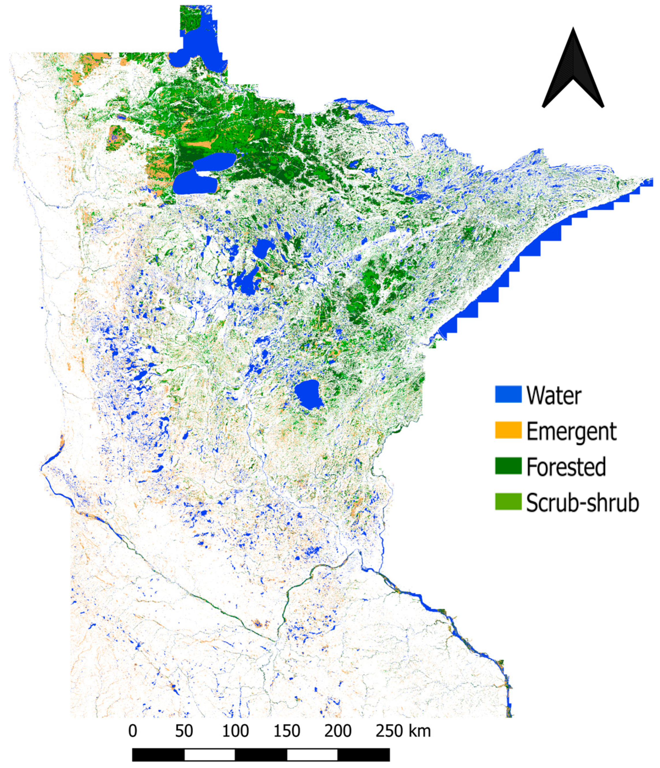
Minnesota, located in the upper Midwest region of the United States (USA), serves as the study area for wetland mapping using remote sensing, as depicted in Figure 1. Covering a total area of 225,000 km2, approximately 20% of Minnesota is comprised of wetlands [3]. Nearly half of the state’s wetlands have been lost since the mid-19th century, primarily due to human activities [3,6]. The majority of wetlands are concentrated in the northeastern part of the state. Emergent, forested and scrub-shrub vegetation classes are prevalent in Minnesota’s wetlands, particularly in the northern and central regions, as shown in Figure 1.
Minnesota experiences an annual precipitation range of 508 to 965 mm, with the highest levels occurring in the southeastern region of the state [27]. The presence of snowmelt and increased precipitation in the spring and early summer leads to higher water content levels in wetland areas [28]. Conversely, during late summer and fall, these areas may experience drying out as water levels decrease. The fluctuation of wetland conditions throughout different seasons significantly impacts the state’s wetland dynamics, adding complexity to the process of wetland mapping, particularly when utilizing remotely sensed data.
3. Data
3.1. National Wetland Inventory Map
The statewide National Wetland Inventory (NWI) map for Minnesota was obtained from the Minnesota Department of Natural Resources (MDNR) as a vector layer. This wetland map was produced using datasets acquired between 2009 and 2014. This product was used in this study as the map from which wetland class information is extracted. The class information is extracted after identifying stable areas, where no significant change is likely to have occurred as will be explained in the method section.
The proposed approach in this study maps wetlands in Minnesota at the class level. In this study, the vector map was rasterized into an image with a 10 m resolution, consistent with satellite imagery resolution, and classified into 4 wetland classes. The unconsolidated bottom, unconsolidated shore, aquatic bed, and streambed classes combined into a single water class due to spectral similarity. The other three classes included emergent, forested, and scrub-shrub wetlands.
3.2. Imagery Input
Level-1C orthorectified top-of-atmosphere reflectance products were acquired through GEE. The imagery was atmospherically corrected in GEE using Sensor Invariant Atmospheric Correction (SIAC) [29]. A median composite was generated for each year from 2016 to 2022, for images acquired between 1 May and 30 June [28]. This time period was chosen as it sees high water content coupled with leaf-off conditions, which enhances the detection of wetlands [28]. Additionally, to streamline the operational process, we focused solely on an aggregate (median) of the data from this period, avoiding the individual monthly information, which would be cumbersome, especially for large-scale mapping. The image collection consisted of ten-meter resolution images of red, green, blue, and near-infrared bands, as well as 20-m red edge 1, red edge 2, red edge 3, red edge 4, short-wave infrared 1, and short-wave infrared 2 bands. To ensure the quality of the images used in the analysis, a filter was applied to select those with a cloud cover of no more than 30%. Subsequently, a cloud mask was employed to eliminate any remaining cloudy pixels from the selected images.
The ability of SAR instruments to operate in any weather condition and around the clock renders them valuable in methodologies in wetland classification, particularly as supplementary sources of information that can be combined with optical data [23]. Although optical instruments capture information regarding the microscopic details of objects, SAR can capture macroscopic details such as information related to geometry, shape, surface roughness, and even moisture content of distributed objects. C-band SAR data is particularly useful for classification of non-forested vegetation [30]. Sentinel-1 data covering the state of Minnesota between 2016 and 2022 in interferometric wide mode and in ascending orbit was accessed through the GEE. To create a composite, the median values of vertical transmit/vertical receive (VV), and vertical transmit/horizontal receive (VH) polarization time-series data were utilized. To further enhance the image quality, a 3 × 3 focal median filter was applied to the composite image to reduce speckle effects [31]. Span and radar vegetation index [32] parameters were calculated from VV and VH data, and used as feature inputs for wetland classification. DEM data and derived products are important features for improving the ability of classifiers to identify and classify wetlands. Elevation and slope calculated from the seamless 1/3 arc-second 3D elevation program (3DEP) product were used as input variables to the model. Table 1 summarizes the imagery datasets used for this study. Additional indices were computed from this imagery data and are summarized in relevant sections.
4. Method
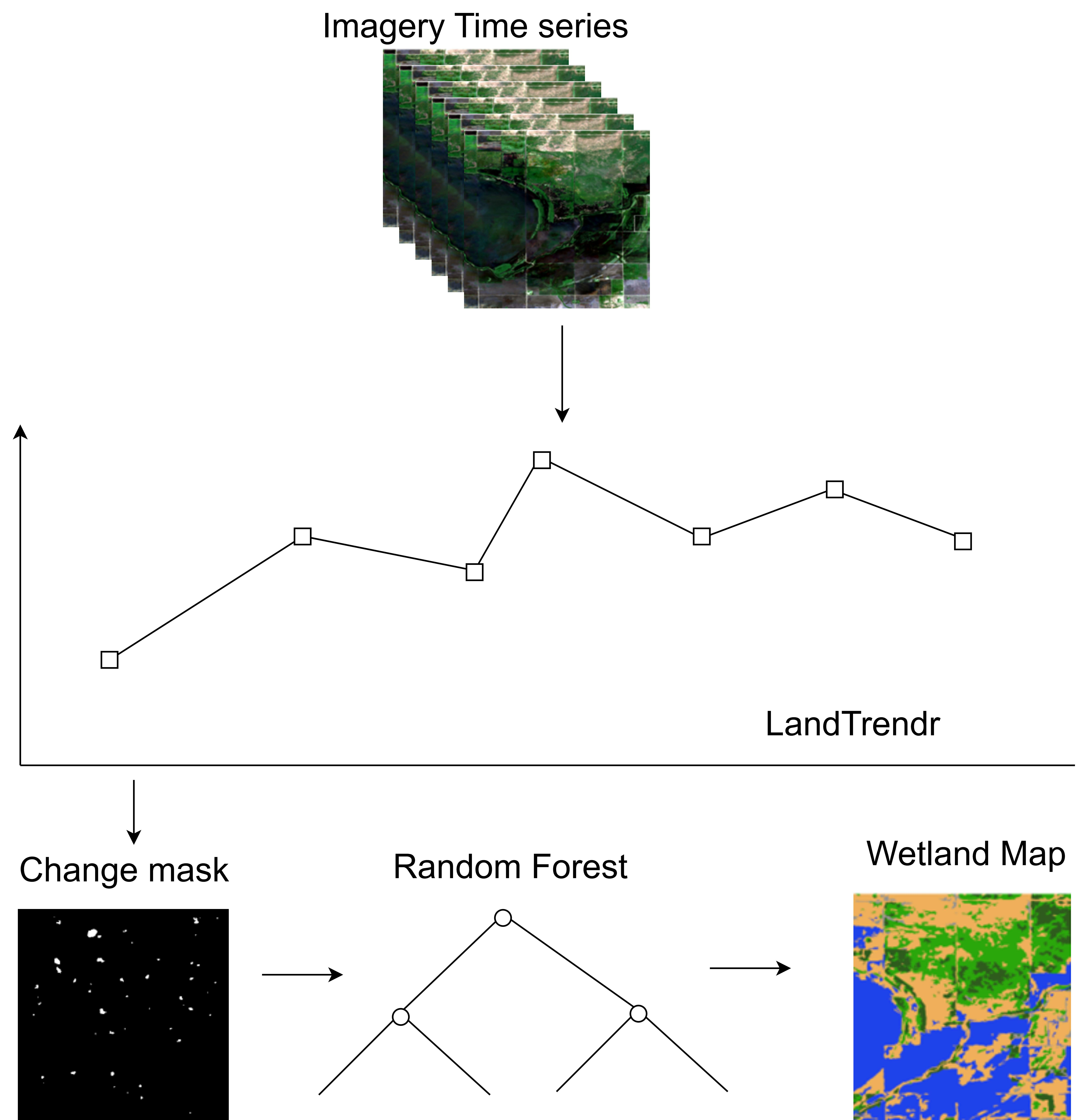
The method used in this study can be described into three main categories. The first category is stable pixels identification. We use stable pixels here to describe the pixels which have not undergone change that would change their land cover class within the 2016–2022 period of interest. Time series remote sensing data is used for change detection, the primary aim of which is to identify areas least likely to have undergone changes that would result in a change in land cover class. The result is a binary mask. In the second stage, the binary mask generated from the initial stage is sampled randomly in ecoregions, and sampled locations intersecting wetland inventory reference dataset are used to extract class labels. Sampling is stratified using ecoregions to ensure that representative samples are acquired from all over the study area.
In the final stage, the sampled locations for which class labels have been extracted are used to extract predictor values of the images corresponding to the year 2022 which is the target year for the final classification map. This stage does not use time series information, it uses only data on the target year of the classification. The predictor values and class labels are used to train an RF classification algorithm in an object-based image analysis workflow [11] to produce an updated wetland inventory map for the state of Minnesota for the year 2022.
4.1. Stable Pixels Identification
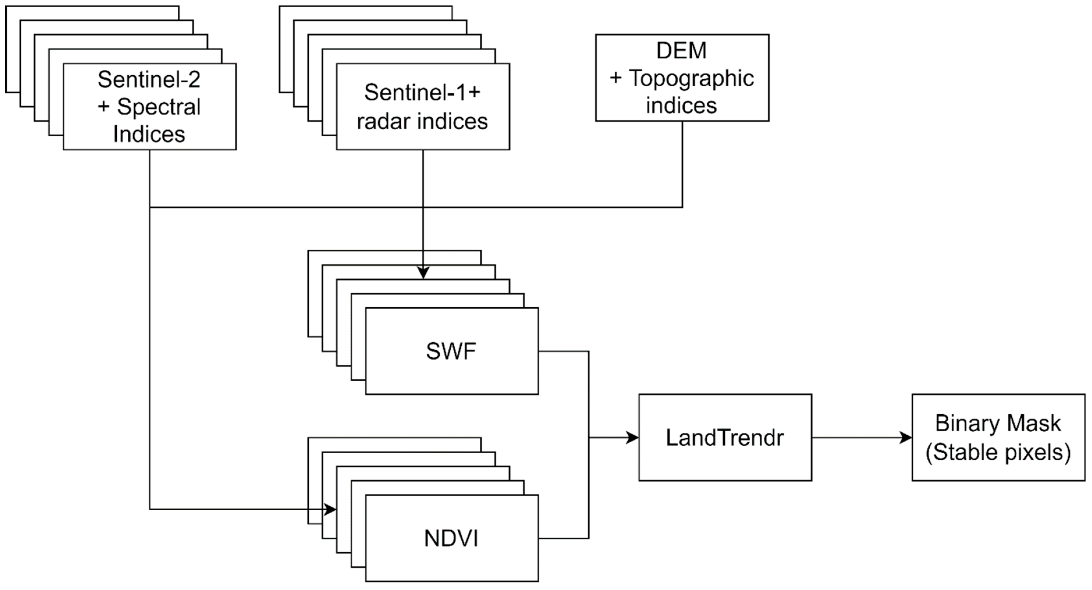
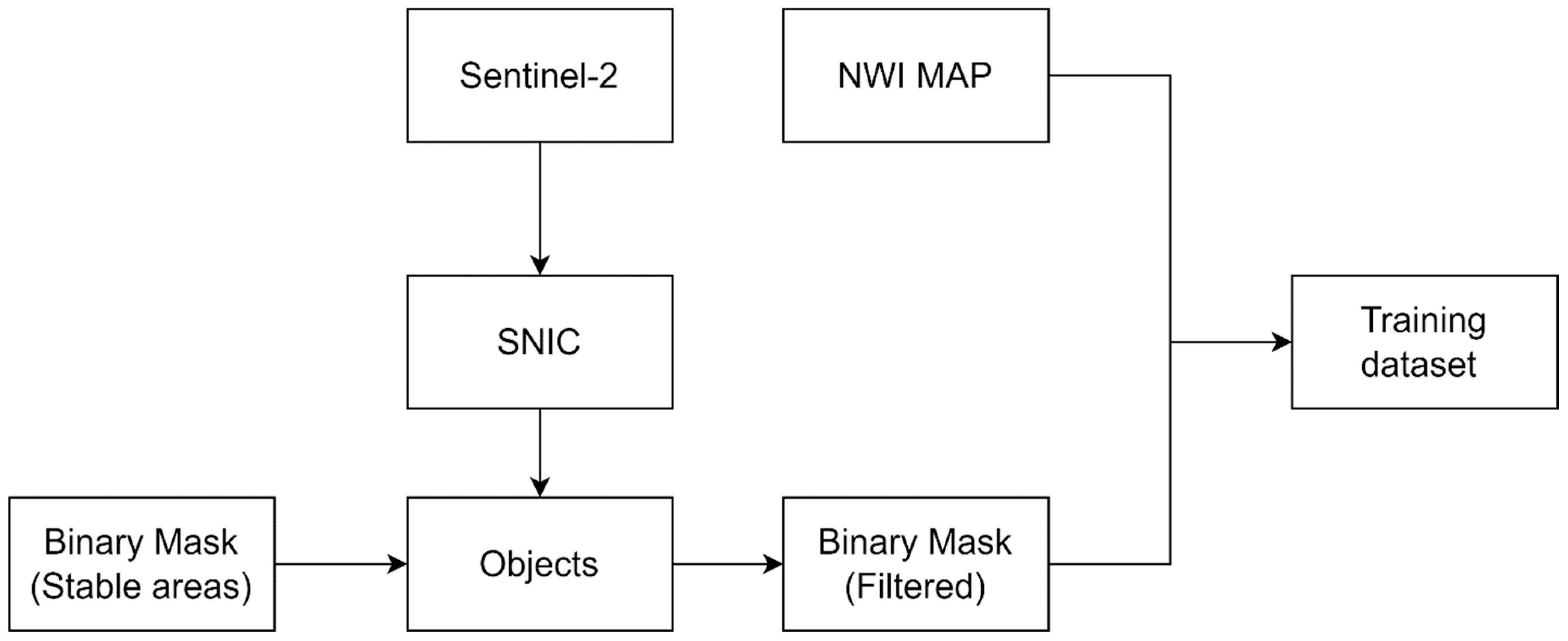
One goal of this paper is to design a dataset generation method, using change detection to identify pixels least likely to have undergone change within a defined period. These “stable” pixels are sampled to generate a dataset for machine learning training. LandTrendr is used as the change detection algorithm to characterize changes in the study area. LandTrendr temporally segments pixel data points, and these segments can be analyzed to understand the changes that have occurred over a period. The change detection algorithm operates on a set of images, one per temporal instant, where an image is representative of the conditions for a temporal instant. Typically, composites are created annually where each image composite represents the conditions of the year [28,33,34,35]. For the purposes of this study, annual composites of the sub-pixel water fraction (SWF) and the normalized difference vegetation index (NDVI) are created as indices characteristic of wetland conditions [28,36]. Although we use change detection in our method to identify stable areas in the study area, the aim of the study is not to show changes in each year in the time series, rather it is to use the stable areas as a data source from which to extract reliable training samples for the purpose of wetland classification. Figure 2 summarizes the process flow and shows the output from this stage.
4.1.1. Sub-Pixel Water Fraction (SWF)
LandTrendr requires one image per temporal instant of a time series to perform temporal segmentation. Depending on the application, different indices are used for characterization in different applications, for instance normalized burn ratio (NBR) is typically used for deforestation studies [33]. In this study, SWF is used as one of the indicators for wetland ecosystems [28,36]. SWF defines the proportion of a pixel that is wet. This ranges from 0 to 1 where 0 means that no fraction of the pixel is wet and 1 indicates the pixel consists of only water. To create an SWF time series, a slightly modified approach for mapping SWF adopted from DeVries et al. (2017) was used [36]. Figure 3 shows the SWF creation process.
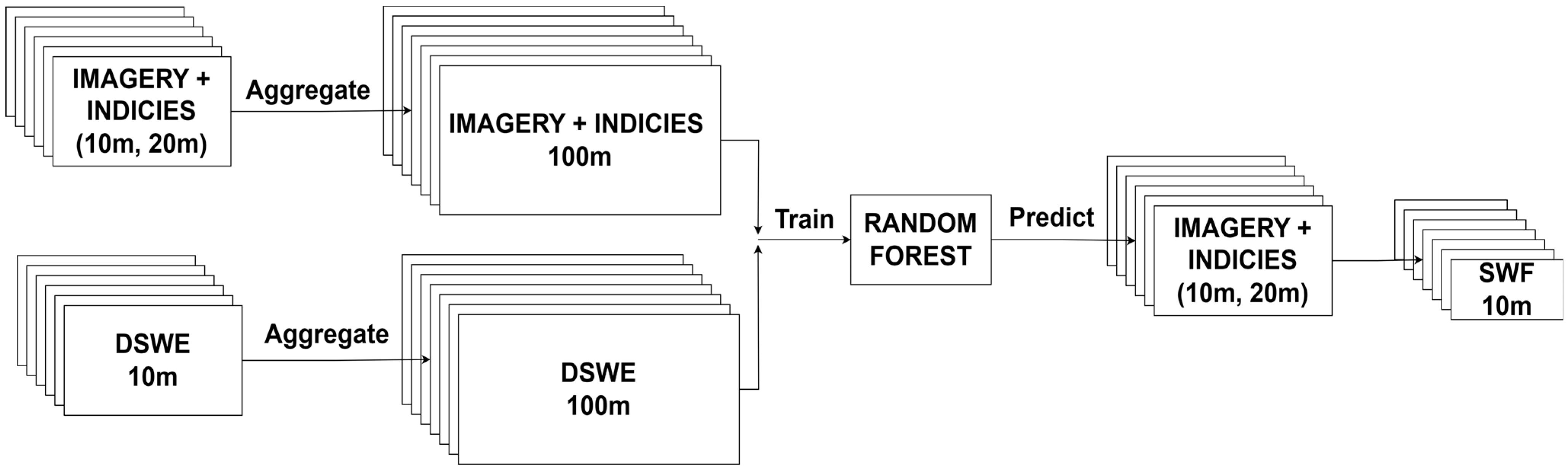
First, dynamic surface water extent (DSWE) maps for each year in the time series were generated using Sentinel-2 multispectral data in GEE [37,38,39]. DSWE maps utilize a categorization system ranging from 0 to 4, where each number represents a different classification for water presence. In this system, 0 indicates no water, 1 represents open water with high confidence, 2 represents open water with moderate confidence, whereas 3 and 4 indicate partial surface water classes. Description of DSWE calculation is provided in Appendix A. DSWE maps were then reclassified into a binary mask indicating water or no-water pixels and aggregated to 100 m resolution by averaging their original 10 m resolution data. The aggregates at 100 m are percentage values indicating the number of water and non-water pixels. For example, an aggregate value of 60% indicates that 60 pixels were water pixels and 40 were not water pixels. This aggregate at 100 m is SWF, i.e., the aggregate value is an estimate of the proportion of the pixel that is wet.
Next, Sentinel-2 data, Sentinel-1 data, elevation data, and derived indices (Table 2 shows a summary of derived indices computed in addition to the input imagery), were similarly resampled to 100 m resolution, and used as predictors for SWF. A random forest (RF) regression model was then trained using the resampled predictors and SWF (aggregated DSWE) both at 100 m. Training samples for fitting the RF model were generated by taking a stratified random sample of 1000 points for every 10% SWF category and for each year in the 2016–2022 time series resulting in a sample of 70,000 points. An estimate of SWF at 10 m is then generated by running inference on the original 10 m bands using the trained model. The process is described as self-supervised because training samples were not created as in supervised classification methodologies for the purpose of training the model, rather an initial estimate of SWF, calculated by aggregating DSWE to a lower resolution, was used as target variable.
It is important that we make a distinction between the RF model trained for the purpose of estimating SWF here and the RF model that will be used for classifying wetlands. Also, although time series image is used for the generation of SWF, only data for target year of map updating was used in the classification process.
4.1.2. LandTrendr
LandTrendr is used to detect and analyze land cover change based on time series remote sensing data [40]. The algorithm detects possible changes in the time series by fitting line segments between pixel observations, representing the change in spectral signature between these points. These segment fits reduce noise, and hence, model significant changes to spectral trajectories. The algorithm works by first despiking spectral values along the time-series. Then it identifies potential vertices. This is achieved using a regression-based vertex identification method. The start and end years are used as initial vertices. Then, least squares regression is calculated for all the points in the time series. The point with the largest absolute deviation is chosen as the next vertex, which segments the data temporally into two segments. The process is repeated for the segments created until the number of segments specified through “max_segments” and “vertexcountovershoot” is reached. Vertices are also removed using a culling curve approach where the vertex with the shallowest angle is removed. This is repeated until segments reach the maximum segments specified. A second set of fitting algorithms is used to identify values that would result in the best continuous trajectory. The P-value for F-statistic estimates is calculated for models fit across trajectories. This provides a basis for comparing segmentation models with different numbers of segments to select the best model. From the breakpoint identification, the slope, magnitude, and duration of each line segment can be calculated and used to characterize the nature of changes that have occurred in a pixel’s spectral history [33]. Table 3 shows LandTrendr parameter values used during temporal fitting; all parameter values used except “max segments” and “min observations needed” were adopted from Lothspeich et al., 2022 [28], as the study area is the same. The maximum number of segments allowed for the temporal fitting and minimum number of observations needed for fitting in the time series used for the purpose of the study were 4 and 6, respectively, considering the fact we have 7 temporal instants of interest.
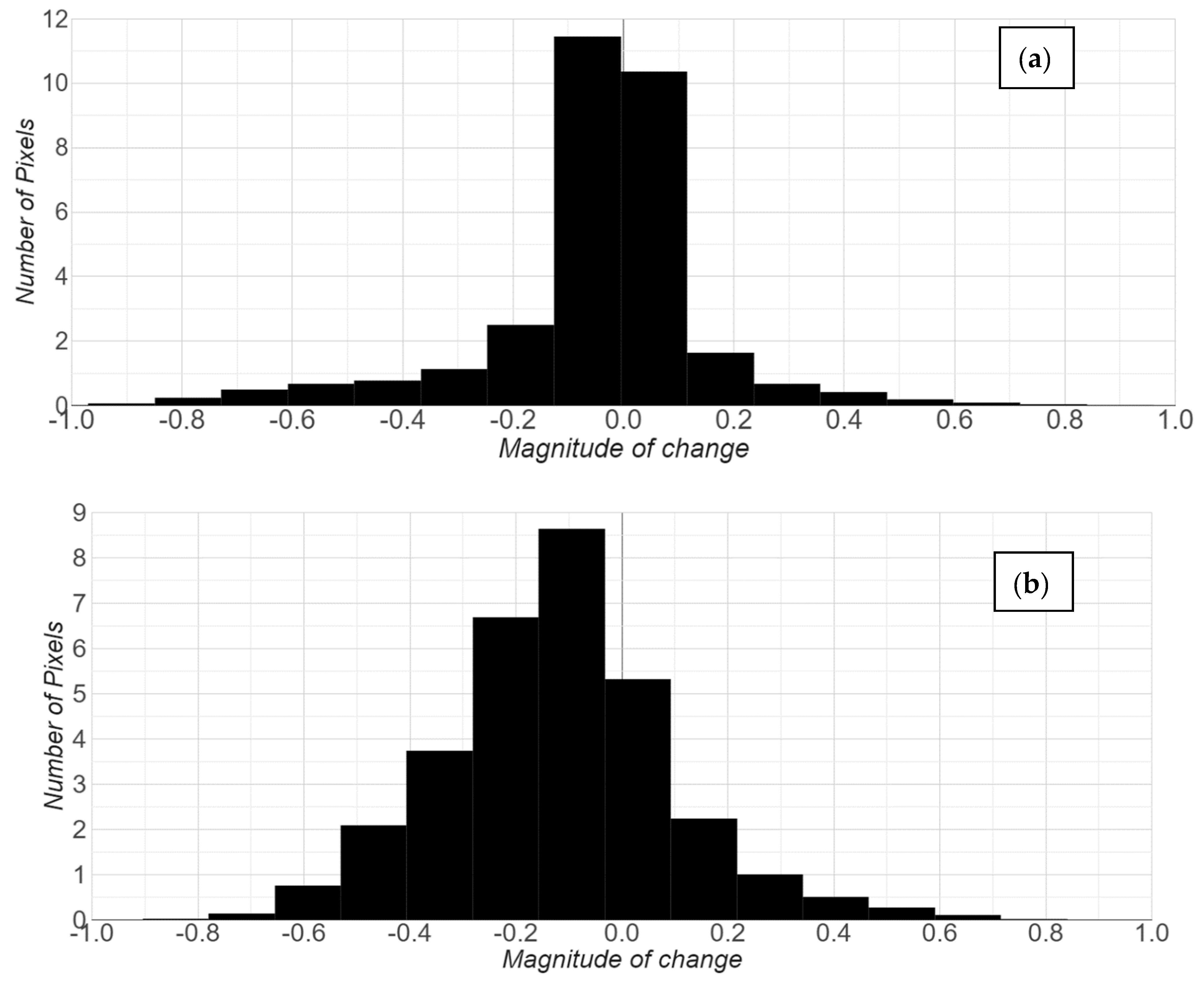
To quantify the magnitude of the changes that occurred in the study area we used, the “getchangemap” function of LandTrendr to analyze the temporal fitting. The histograms in Figure 4 show the magnitude of change in the study area scaled down by a factor of 108. The range of magnitude of change was limited to a range of −1 to 1, where the negative sign indicates loss and positive signifies gain. After producing the magnitude of change images, we use a trial-and-error method to determine unchanged area cut-off threshold. This was done by visually inspecting known wetlands and large bodies of water, and testing 0.01, 0.02, 0.05, and 0.1 as threshold for magnitude of change. We selected a threshold of 0.05 after this trial-and-error and visual inspection. This threshold is very conservative in order not to choose unreliable samples, but it also contains enough stable areas for model training sampling.
4.2. Training Sample Selection
Figure 5 describes the process flow for the training sample selection stage. To further boost the consistency of training sample selection, unchanged pixels which did not make up more than 50% of object clusters were filtered out. Also, objects which had more than 50% of constituent pixels classified as unchanged were assumed to be unchanged. Objects refer to coherent regions or clusters within an image that share similar spectral, texture, shape, and spatial characteristics. Objects were created for the study area by applying a simple non-iterative clustering (SNIC) [41] algorithm on GEE. The SNIC algorithm works by non-iteratively updating cluster centroids [42]. The algorithm initializes superpixel cluster centroids on a regular grid. A distance metric centroid using spatial and color measures is used to measure the distances of pixels to the cluster centroid. The algorithm uses a priority queue to choose pixels to add to a cluster. The priority queue comprises candidate pixels that have 4 or 8 connectivity to a superpixel cluster. The pixels in the queue with the shortest distance are chosen. This pixel is then used to update the centroid value of the superpixel cluster. This process is repeated until the priority queue is empty, and all pixels have been assigned to a cluster centroid.
After applying the object filtering step, we have a final binary mask indicating unchanged areas. It is important to note here that objects were not generated for all images in the time series, rather it was only generated for the year 2022 which is the year of interest for wetland map update.
To obtain training samples for our wetland classes of interest, the reference NWI layer was sampled in ecoregion level III region, for pixels that intersect unchanged binary mask. To prevent overestimation of wetland classes, upland samples were added using the national landcover database product for 2019 [43]. Upland is used here to refer to non-wetland classes. Samples were extracted for developed, forested upland (deciduous, mixed, and evergreen forest, and scrub-shrub), and agriculture (herbaceous, pasture, and cultivated crops) upland classes. A total of 50,000 samples per class were extracted in each of the 7 ecoregions resulting in a database of approximately 350,000 samples per class.
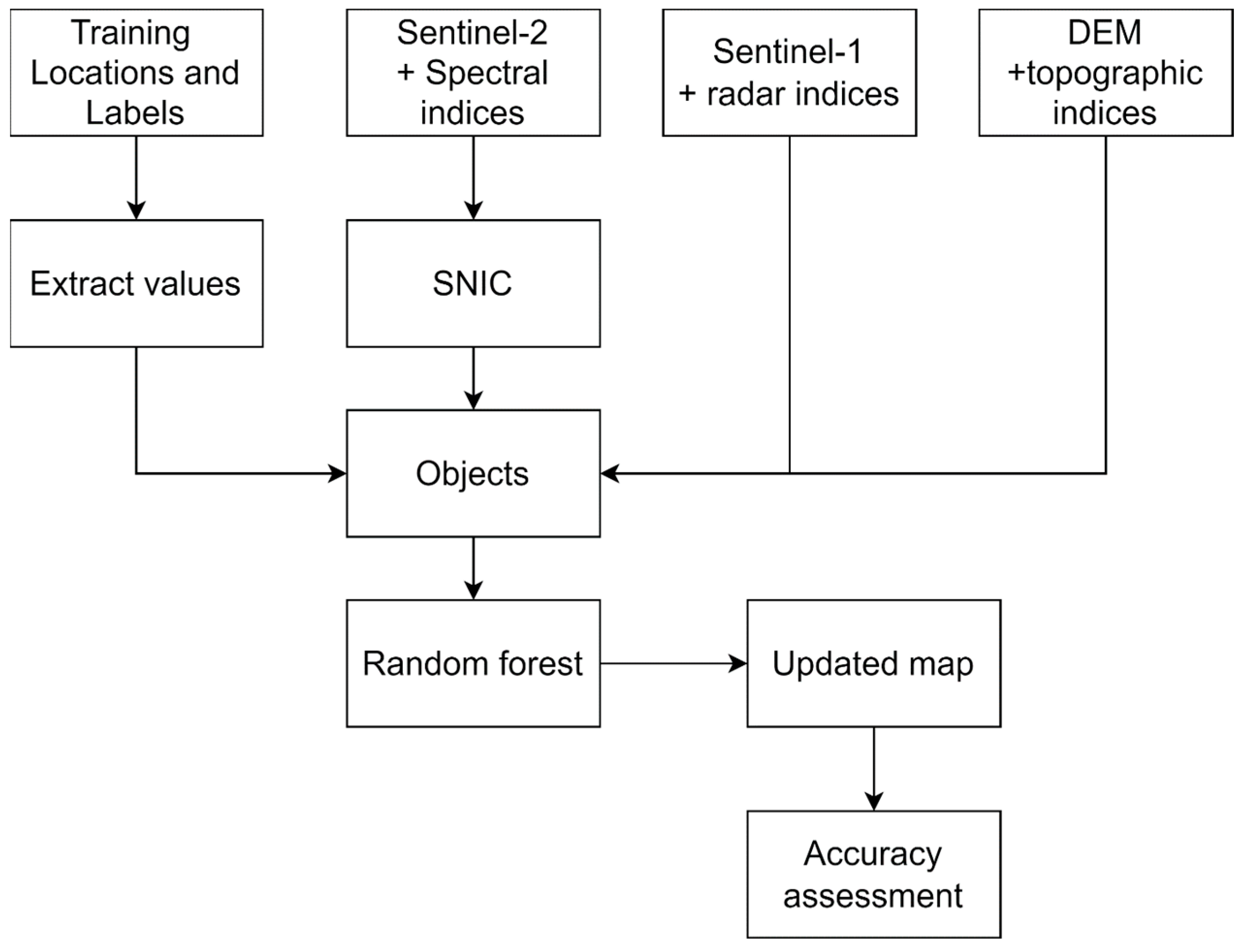
4.3. Classification
In this step, as shown in Figure 6, we carry out classification of wetlands for the state of Minnesota for the year 2022 using a median image composite of Sentinel-1, Sentinel-2 data, and DEM data, and training samples generated in the previous step. Derived indices from Sentinel-1, Sentinel-2, and DEM data for the purpose of classification are summarized in Table 4. The classification step adopts an object-based image classification methodology. Numerous studies have shown the benefits of applying OBIA for the wetland mapping [11,44,45]. OBIA allows for the integration of multiple data sources, such as spectral, spatial, and contextual information, to improve accuracy and reduce classification errors. By grouping pixels into meaningful image objects, OBIA also reduces the effect of spectral variability within an image, making it easier to distinguish different land cover or wetland types [45]. In GEE, the SNIC algorithm is used to create objects as described in the training sample selection section. Input images were transformed from pixel-level to object-level by aggregating pixel values that fall within each object using an averaging operation.
Predictor values for each of the training sample set were then extracted for training a RF model for the purpose of classification. RF is an ensemble of weaker independent decision trees [46]. Each tree is trained on a variation of the entire data, splitting data points based on features that provide the most information gain. Data points are repeatedly split until there is no information gained. Each tree develops a set of rules based on the predictor variables and their predictions are combined using a bagging ensemble technique to come up with final prediction classes. The RF classifier was preferred over conventional classifiers due to its distinctive features, such as the absence of assumptions regarding the underlying data distribution, suitability for managing high-dimensional data, and ability to model non-linearities in the data [7]. The RF classifier was initialized with 250 trees and trained using samples extracted during the training sample selection stage. RF classifier was then applied to input images, aggregated to object-level, to produce statewide wetland map. The final map is of 10 m resolution.
Accuracy Assessment and Evaluation Metrics
To assess the performance of the model and compare it with a baseline, we created an independent test set. The baseline follows the same steps as the proposed method, except in this case we do not apply a sample filtering step. The test set comprises approximately 6300 samples, with an average of 900 samples per class. The samples were generated randomly from each ecoregion, and visually interpreted using NWI map product and remote sensing data. Also, for quantitative comparison of wetland predictions for the years 2021 and 2022, the database of pixels (~2 million data points) is divided in a 60:40% ratio, where 40% of the data served as a validation set.
Overall accuracy, F1-score, user’s, and producer’s accuracy metrics were used to evaluate the performance of the different models. Overall accuracy measures the total number of correctly classified labels.
F1-score: It is the harmonic mean of producer and user accuracy, which considers both false positives and false negatives. This makes the F1 score a useful metric when dealing with imbalanced datasets where one class might be significantly more prevalent than the other.
Producer’s Accuracy (PA): It measures the percentage of correctly classified instances among all instances that were predicted to belong to a specific class.
User’s Accuracy (UA): It measures the percentage of correctly classified instances among all instances that belong to a specific class.
The equations for the metrics are formulated as below:
where TP is true positive, FP is false positive, FN is false negative, UA is the user’s accuracy, and PA is the producer’s accuracy.
5. Results
5.1. Quantitative Assessment
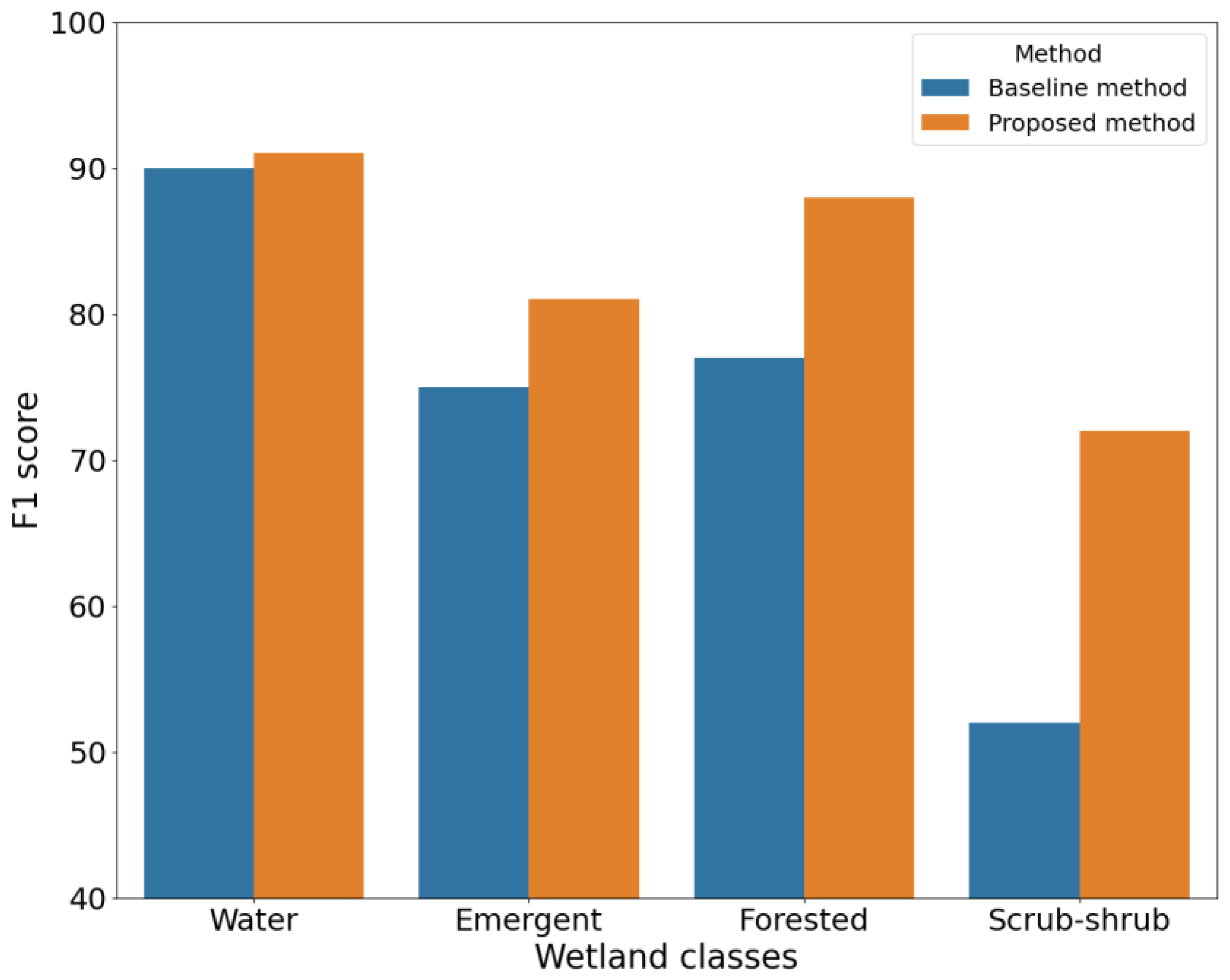
Table 5 compares the confusion matrices for performance of baseline approach and the proposed method. The proposed method is seen to perform better than the baseline method, especially for complex wetland classes. In both cases we see that scrub-shrub class is the most difficult class to predict with true positive predictions at 49% and 68% for baseline method and proposed method respectively. Table 6 further summarizes results from Table 5 into producer’s and user’s accuracies, and F1 scores.
The overall classification accuracy of wetlands was determined by applying the model to the test set and was found to be 89%. This indicates that the classification algorithm performed well in accurately distinguishing between wetlands and uplands. We were able to identify wetlands 84% of the time and uplands 94%, as reflected in wetland–upland producer accuracies. To further evaluate the accuracy of wetland classification, overall accuracies and class-based producer and user accuracies, as well as F1 scores for each sub-class of wetlands were calculated. For the wetland classes, the water, emergent, forested, and scrub-shrub classes had F1 scores of 91%, 81%, 88%, and 72%, respectively.
A similar methodology without the training sample selection process was carried out to establish a baseline to compare the proposed method with. Quantitative assessment on both methods is reported in terms of overall accuracies and class-based producer and user accuracies, as well as F1 scores. Table 6 summarizes the results.
The proposed method performed better in terms of F1 scores, producers’, and users’ accuracies. We observed a 7% jump in overall accuracy when applying the proposed method to discriminate classes. A clear difference is noticed when the wetland samples are analyzed. The baseline method identified wetlands 75% of the time, and 69% if the wetland classes are non-open water, compared to 84% wetland identification and 82% when non-open water classes are considered for the proposed approach. An average improvement of about 13% for non-water wetland classes and 2% for water class is observed. This is due to the ability of the methods to capture short-term changes that have occurred in the area of study. Figure 7 shows F1 score comparison for wetland class prediction between baseline method and proposed method.
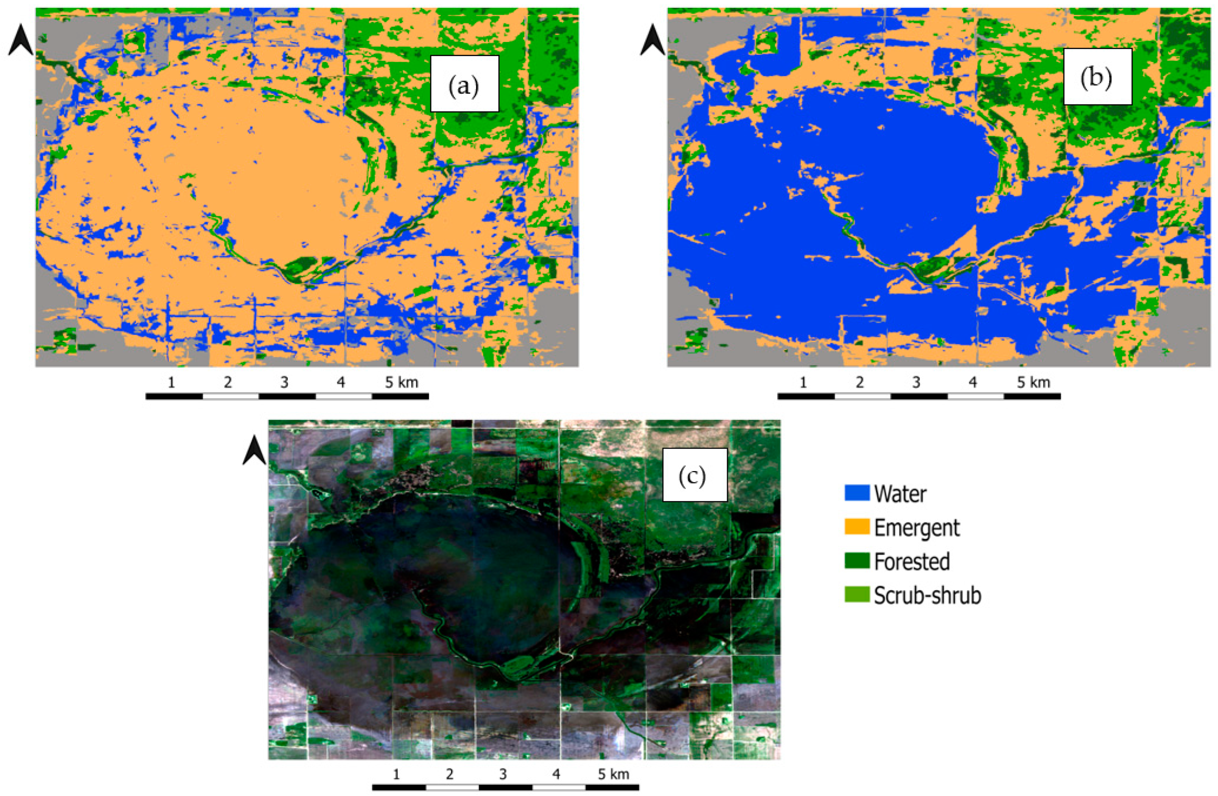
Figure 8 provides a visual comparison of baseline and proposed method predictions. The patch visualized was flooded in 2022 as seen in the Sentinel-2 image in Figure 8c. The proposed approach performs better than the baseline method in classifying the wetland features in this patch.
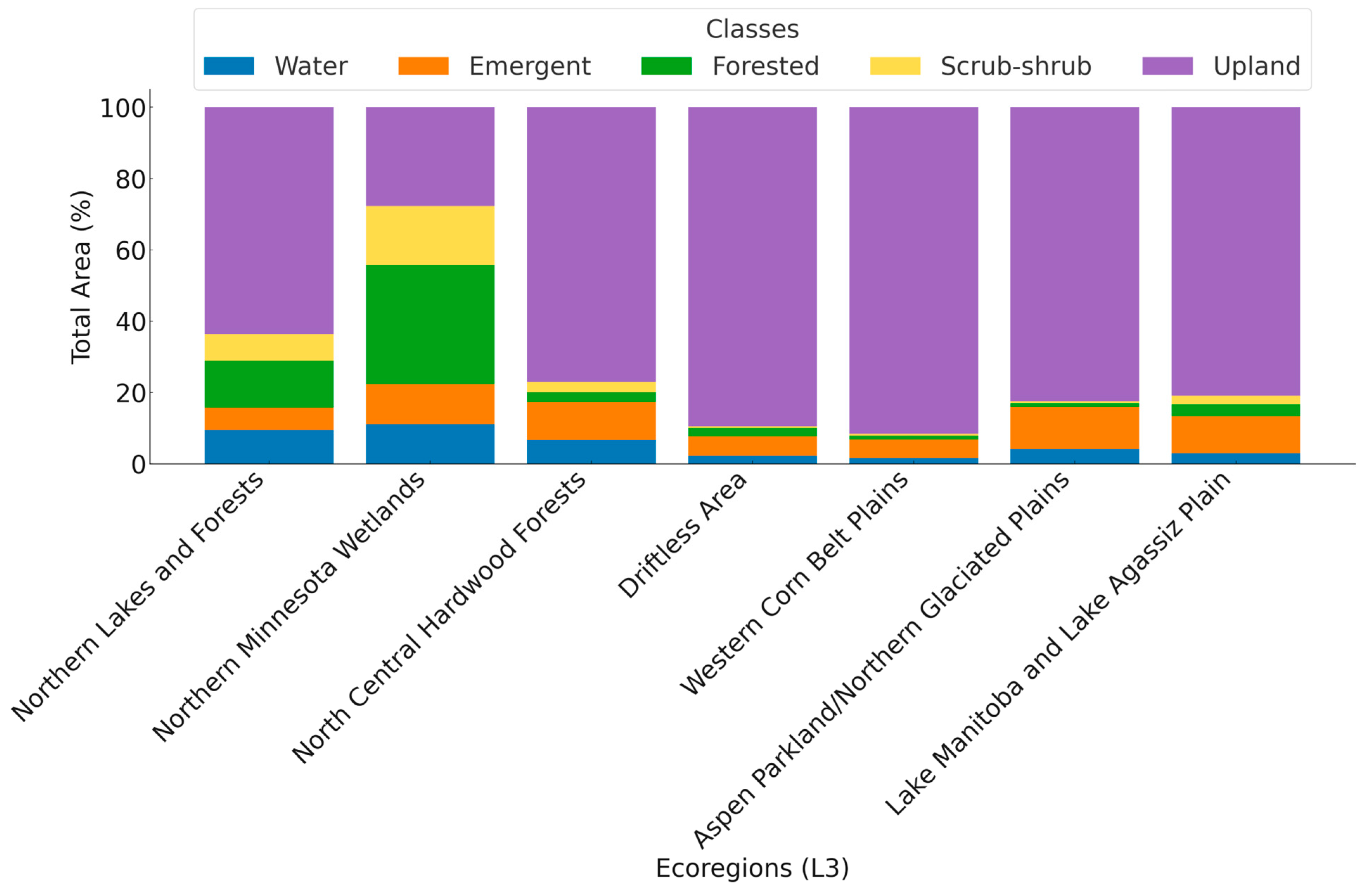
Across Minnesota, the results estimate that the state’s wetland (non-open water) constitute about 21% of the state. Figure 9 and Figure 10 summarize the distribution of wetlands across the state for each class. Analyzing the distribution of wetlands across ecoregions, Northern Minnesota stands out prominently in wetland coverage, with the “Northern Lakes and Forests” and “Northern Minnesota Wetlands” ecoregions collectively accounting for approximately 60% of the total wetland area. Specifically, the “Northern Minnesota Wetlands” region is predominantly characterized by forested wetlands, constituting 33.32% of its composition, whereas the “Northern Lakes and Forests” region presents a more balanced distribution among wetland types. Conversely, regions such as the “Western Corn Belt Plains” and “Driftless Area” are dominated by upland classifications, representing over 89% of their total wetland area.
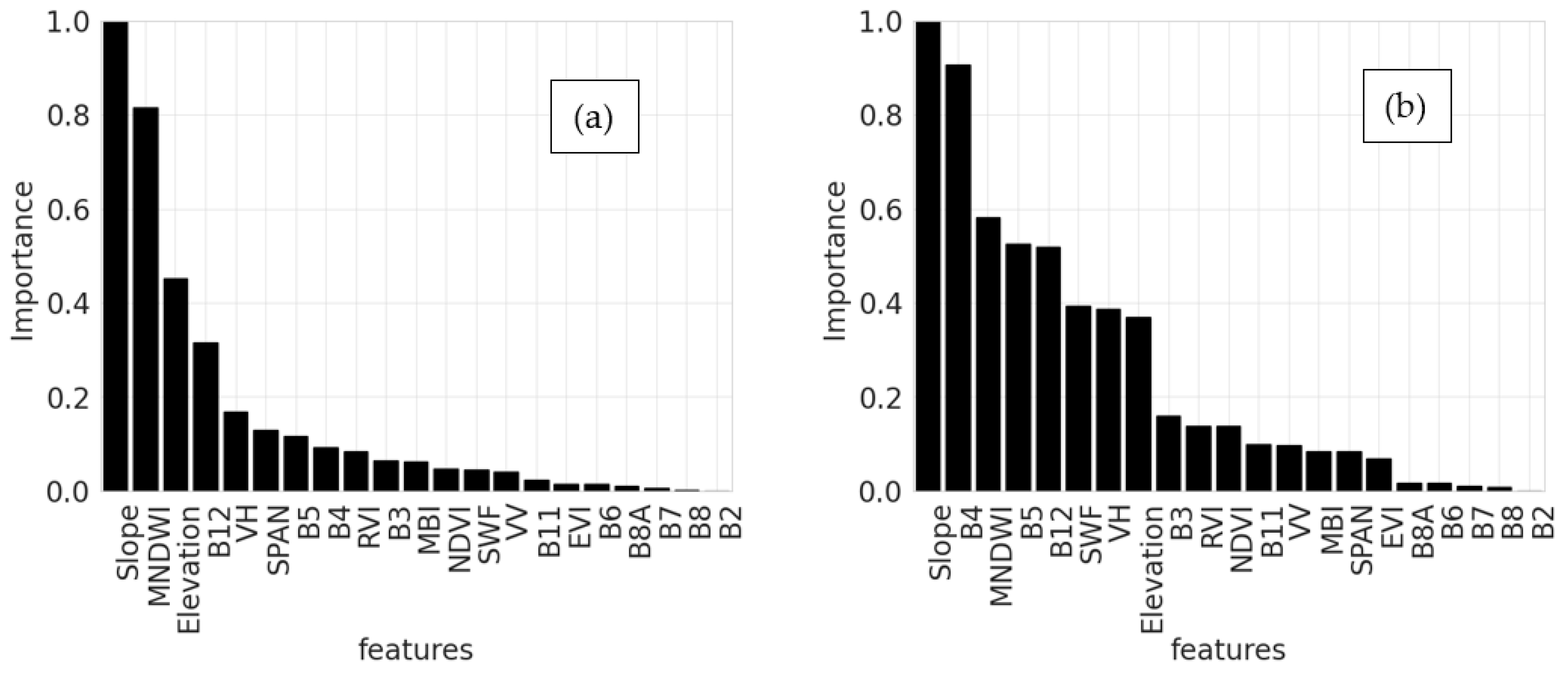
In our wetland classification, the primary determinants were slope, B4, MNDWI, B5, B12, SWF, VH and elevation. B3, RVI, NDVI, B11, VV, MBI, SPAN, and EVI also contributed to the discrimination power of the model. The features B8A, B6 B7, B8 and B2 had relatively low impacts on the model performance. We were particularly interested in seeing the significance of the SWF index and how it is impacted by increased water content due to events such as flooding. We analyze this index in the following section. We attempt to isolate the impact considering two years, one with high water content due to flooding events (2022) and the other with low water content due to drought (2021).
5.2. Effect of SWF Index
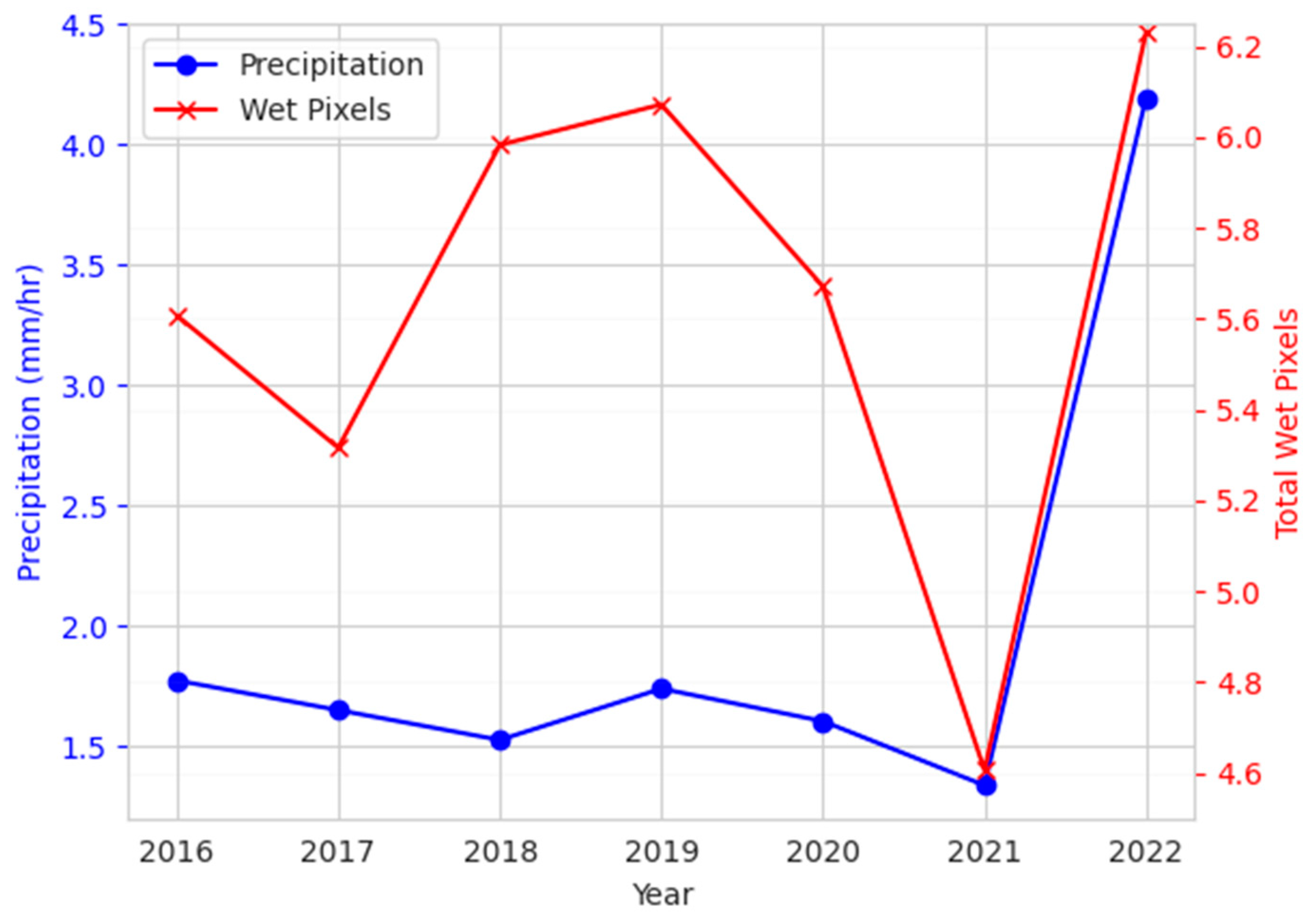
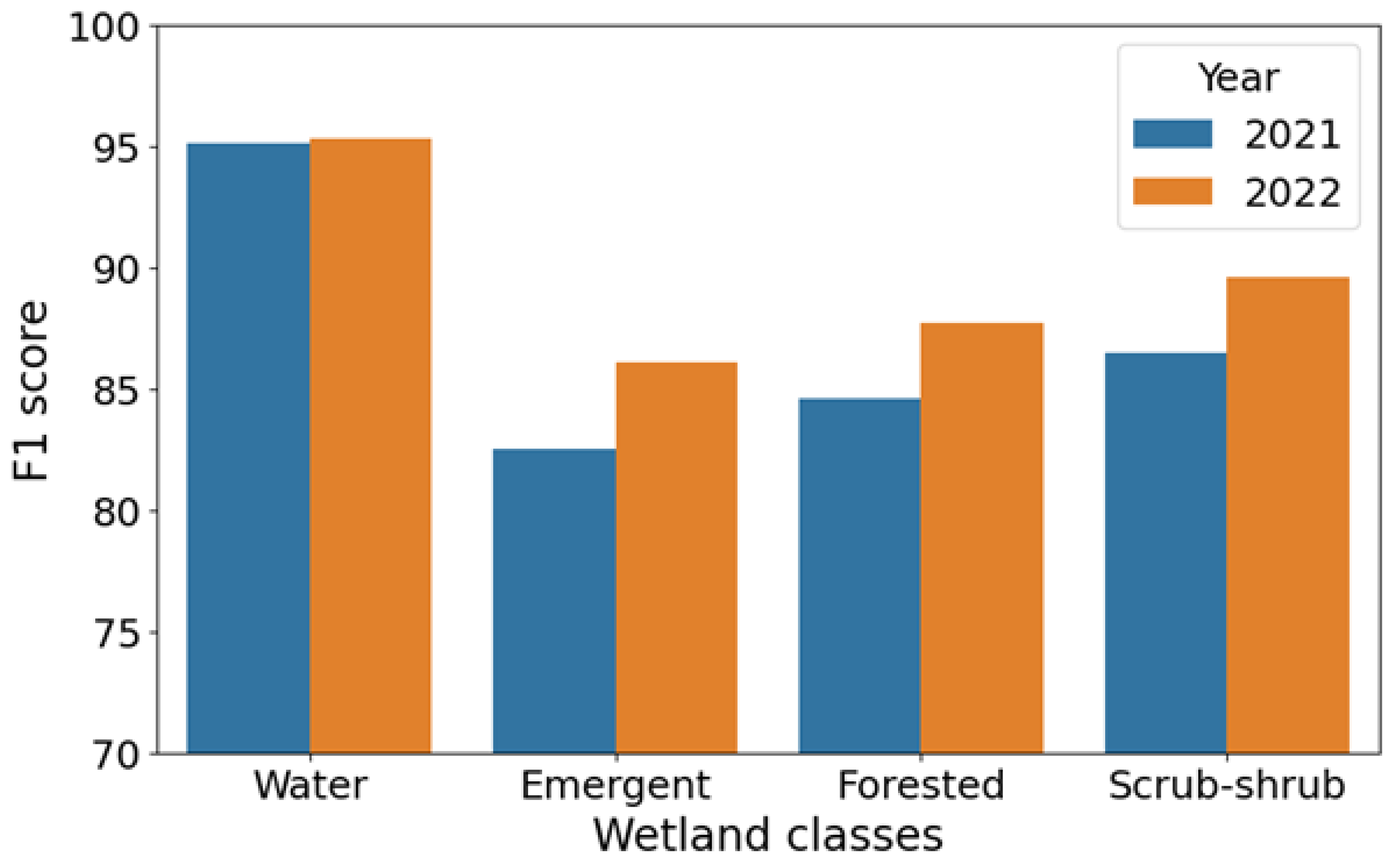
To assess the effects of SWF index in the classification process, we apply the proposed method for the year 2021; using the same training samples (which has previously been determined to be stable over the time series). This was done because there was a drought in 2021 in Minnesota and flooding in 2022, hence, more pixels had higher SWF values in 2022 in comparison to 2021. Figure 11 summarizes a trend in precipitation and high SWF values (we considered SWF > 0.5 to be high values [28]). Comparing performance on the validation set, there is a 2% decrease in overall wetland classification accuracy when the wetland inventory map is produced for 2021; performance was assessed on validation set. Breaking down to class-based metrics, Figure 12 shows a bar chart comparing the wetland classification F1 scores for 2021 and 2022. The model produced for 2022 performs better across the wetland classes. The emergent class was impacted the most, with an F1 score decrease of 4%. SWF also dropped a few places in the importance ranking of features used by the RF classifier as shown in Figure 13. This may be due to the reduced water content in 2021 making the SWF index relatively less useful for discriminating wetland classes in comparison to the year 2022.
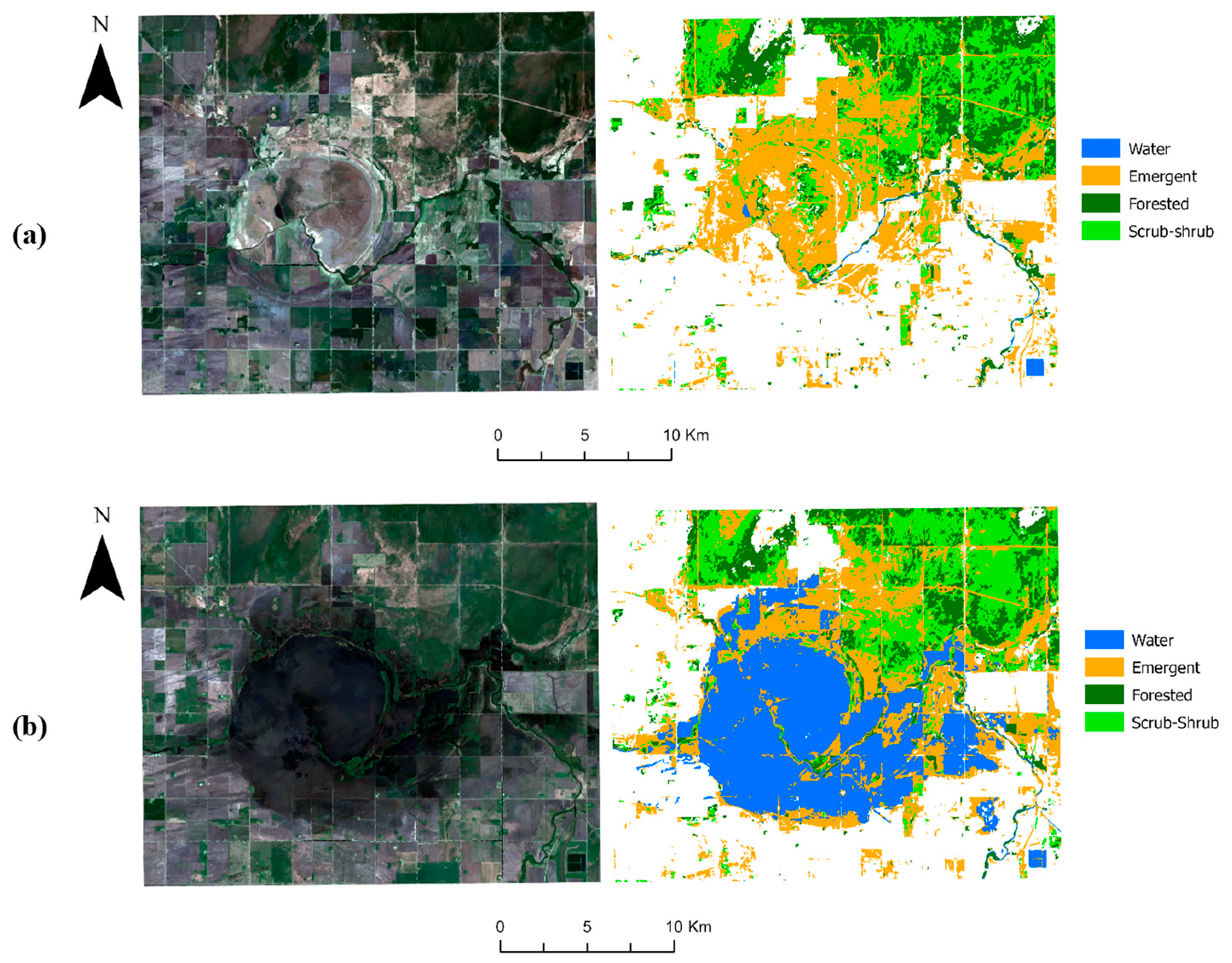
Visual inspecting of images in Figure 14, we see that wetland labels are dynamic. A common occurrence is emergent water change due to a rise in water content. These results suggest that flooding has significant impacts on wetland mapping. On one hand, flooding can increase the amount of water content, which can make it easier to detect wetlands from satellite remote sensing. On the other hand, flooding can also cause wetlands with little or no vegetation cover to change their appearance temporarily or seasonally. Wetland dynamism highlights the need for regular inventory updates.
6. Discussion
The comparison between the baseline and proposed methods across different wetland and upland classes reveals substantial improvements in accuracy. The proposed method, employing a change detection technique to filter training samples, shows enhanced accuracy in various classes. This approach leverages the identified stable areas for training samples selection, thereby enhancing the quality of the training dataset for machine learning. Consequently, this method attains better results for all classes. The higher accuracy in wetland classes, such as emergent (PA: 88%, UA: 76%) and forested (PA: 89%, UA: 87%), underscores the efficacy of this strategy in mitigating spectral confusion, thereby achieving more accurate classification. This observation extends to upland classes as well, with urban (PA: 100%, UA: 99%), forested (PA: 92%, UA: 93%), and agriculture (PA: 91%, UA: 98%) classes also benefiting from the refined training dataset. This systematic approach, guided by training sample filtering through change detection, offers potential avenues for improving remote sensing-based classification strategies.
The accuracy of the map produced is 89% which is comparable to previous wetland mapping studies [7,47,48,49,50] especially large scale wetland studies in Minnesota [51,52]. This study leverages Sentinel-2 and Sentinel-1 data for wetland mapping. The integration of multisource data, Sentinel-2, and Sentinel-1, improves wetland classification [11,48,52]. Additionally, the adoption of OBIA helps to further minimize spectral variability within classes, enhancing mapping accuracy [53]. Water bodies achieve high accuracy (PA: 90%, UA: 93%), attributed to distinct spectral signatures. Conversely, emergent wetlands (PA: 88%, UA: 76%) suffer from spectral confusion due to varied vegetation types, like scrub shrubs. Forested wetlands share spectral and structural resemblances with forested upland, leading to misclassification. Spectral similarity also impacts scrub-shrub (PA: 68%, UA: 76%) and emergent (PA: 82%, UA: 88%) classes. Scrub-shrub wetland class especially share similarities with forested wetland, emergent wetland, and forest upland classes leading to low classification accuracy.
6.1. Dataset Generation Using Change Detection
To achieve successful training for wetland mapping using remote sensing, it is crucial to have a substantial training dataset that encompasses a diverse array of class variations [50]. The size of the study area also plays a critical role in determining the number of required samples [50]. Additionally, acquiring representative samples of wetlands can be particularly challenging due to their spatial extent and ecological complexity [50]. Therefore, to ensure reliable wetland mapping, it becomes imperative to ensure that the collected samples comprehensively capture the full range of variability present within wetland ecosystems. However, various challenges like the intricate nature of wetlands, expansive study areas, and other limitations make it impractical to conduct extensive field campaigns to collect a sufficient quantity of labeled samples within a reasonable timeframe. To solve this problem, studies identify areas least likely to have changed leveraging time series data and change detection [21,22].
In our study, we developed an innovative approach for generating a robust dataset. This method capitalizes on existing wetland inventories and employs change detection techniques applied to time series remote sensing data. By combining these resources, we created a sizable dataset containing around 1.2 million samples, which corresponds to approximately 5% of the total study area. Our dataset creation strategy was further refined by filtering out labels with a low chance of being associated with objects to ensure consistency. Also, by employing a sampling strategy at the ecoregion level, we facilitated the inclusion of samples that exhibit a broad spectrum of variations within the database. Additionally, this technique ensured that our database comprised representative samples in equal proportions across different categories, addressing the need for capturing variability. This meticulous process was instrumental in enhancing the accuracy and reliability of our wetland mapping results.
6.2. Effect of SWF Index
Minnesota experienced a significant shift in precipitation patterns in 2022 compared to the previous year [54]. Above-average precipitation was recorded at monitoring stations across the state, with the wettest conditions concentrated in northwestern, northern, and northeastern parts of Minnesota. Some areas received two to five times the precipitation compared to the same period in 2021 [54]. Parts of the state that were severely impacted by drought in 2021 saw an extremely wet spring in 2022, leading to high water tables and flooding in some areas. Flooding was caused by snowmelt and precipitation. These changes in precipitation patterns highlight the variability and extreme weather events that can occur in Minnesota and their impacts on hydrological systems in the state. Flooding can have significant effects on wetland mapping as an increase in water content could improve detection of wetlands from satellite remote sensing. Corcoran et al. (2011) explains that lots of wetlands occur for short periods and could be missed in inventories due to timing of imagery acquisition [51]. Figure 12 shows that wetland classification improves when SWF values are higher. Also, analyzing Figure 12 together with Figure 13, higher SWF values make the SWF index important for the classifier which in turn improves wetland class discrimination. If water content increases for a wetland pixel, the SWF value will increase for that pixel, increasing the likelihood of it being identified as a wetland from satellite remote sensing methods.
6.3. Scalability
The proposed method is scalable as is seen in the application of the approach to Minnesota which is about 225,000 km2 in area. However, structural limitations placed by GEE need to be considered when planning to adopt the method based on the size of the area of study and size of the database that would be used to train a model. The use of GEE as a remote sensing platform for rapid wetland map update has numerous advantages, including access to a vast amount of satellite imagery and powerful processing capabilities [13]. However, there are several limitations that must be considered when using GEE for training large sample sizes in remote sensing studies. Despite its powerful processing capabilities, GEE has some limitations in terms of processing time and resource allocation. Training large sample sizes requires significant computational resources, including storage and processing power, which may exceed the limits placed by GEE. This can result in longer processing times or incomplete processing, leading to potential limitations in training large sample sizes. Utilizing graphical processing units (GPUs) significantly reduces the training and inference times and has significant impacts on large-scale updates of landcover inventories using remote sensing data. cuML RAPIDs [55] is used to train our RF model on GPU. Comparing inference times for the study area comprising 120 inference patches each 7168 by 7168 and 21 bands split equally across three machines, inference time on GPU was about 1 h 30 min compared to 7 h on CPU.
The applicability of this method to other projects depends on multiple factors including, the presence of an existing map product for the target study area, the study area’s size, and the temporal gap between the creation of the original map and the intended production date of the new product. The size of the study area influences the quantity of labeled samples that can be extracted. Larger areas typically offer sufficient training samples, even after applying sample filtering. Also, a significant time lapse might suggest potential complex changes, necessitating advanced sample filtering techniques and the availability of extended time series remote sensing data.
7. Conclusions
Reliable samples for training models to predict classes remain an important consideration in the production of landcover maps. Limitations imposed by field data collection or image interpretation require alternative methods for map production, especially for large areas, such as state-wide mapping. Training models on a large database of samples extracted from an existing wetland thematic map is an effective way to update wetland inventory maps. In this study, we find that using time series information, we can filter an existing thematic map to produce reliable training sets for inventory updates.
Using LandTrendr, the proposed filtering process for selecting training samples improves the discrimination of wetlands from upland classes as well as the ability to distinguish different wetland classes. LandTrendr proved to be particularly useful for modeling short-term changes in wetland indicators, such as the identification of flooded areas in northern Minnesota. We also see in this study that increased water content through events such as flooding can boost classification of wetlands from remote sensing approaches, and events are seen to improve wetland classification accuracy, but it is also seen that it can change the land cover labels of the wetland area especially for wetland ecosystems with short cover. Dynamism of wetlands highlights the need for regular updates of wetland inventories. The proposed method can be adapted for producing frequent wetland inventory maps in multiple cycles during the year. Improvements in result can be achieved either by using iterative sample filtering approaches to refine the training sample database or post-processing to edit labels generated. Deep learning methodologies could also be used to take advantage of the extensive database of generated samples.
Author Contributions
Conceptualization, V.I., B.S. and M.M.; Data curation, V.I.; Formal analysis, V.I. and M.M.; Methodology, V.I., B.S. and M.M.; Software, V.I.; Supervision, B.S. and M.M.; Visualization, V.I.; Writing—original draft, V.I.; Writing—review and editing, V.I., B.S. and M.M. All authors have read and agreed to the published version of the manuscript.
Funding
This research received no external funding.
Data Availability Statement
Data available on request to the authors.
Acknowledgments
Special thanks to the Minnesota Department of Natural Resources for making the wetland inventory data used in this study publicly available.
Conflicts of Interest
The authors declare no conflict of interest.
Appendix A
Five conditions are tested and based on the outcome, we set a distinct bit in a 5-bit number.
The following are the conditions and corresponding values.
- Test 1: If (MNDWI > 0.124) set the ones digit (i.e., 00001)
- Test 2: If (MBSRV > MBSRN) set the tens digit (i.e., 00010)
- Test 3: If (AWESH > 0.0) set the hundreds digit (i.e., 00100)
- Test 4: If (MNDWI > −0.44 && B5 < 900 && B4 < 1500 & NDVI < 0.7) set the thousands digit (i.e., 01000)
- Test 5: If (MNDWI > −0.5 && B5 < 3000 && B7 < 1000 && B4 < 2500 && B1 < 1000) set the ten-thousands digit (i.e., 10000)
After setting the values, the following values are assigned to each pixel:

Table A1.
Table summarizing values assigned to each pixel based on the 5-bit value.
| Value Assigned | Bit Value |
|---|---|
| Not Water (0) | 00000 |
| 00001 | |
| 00010 | |
| 00100 | |
| 01000 | |
| Water—High Confidence (1) | 01111 |
| 10111 | |
| 11011 | |
| 11101 | |
| 11110 | |
| 11111 | |
| Water—Moderate Confidence (2) | 00111 |
| 01011 | |
| 01101 | |
| 01110 | |
| 10011 | |
| 10101 | |
| 10110 | |
| 11001 | |
| 11010 | |
| 11100 | |
| Potential Wetland (3) | 11000 |
| Low Confidence Water or Wetland (4) | 00011 |
| 00101 | |
| 00110 | |
| 01001 | |
| 01010 | |
| 01100 | |
| 10000 | |
| 10001 | |
| 10010 | |
| 10100 |
Also, the following four conditions are tested, and values assigned to get the final DSWE:
- If (percent-slope >= 30% slope) and the initial DSWE is High Confidence Water (1), the final DSWE is set to 0 otherwise set it to initial DSWE;
- If (percent-slope >= 30% slope) and the initial DSWE is Moderate Confidence Water (2), the final DSWE is set 0 otherwise set it to initial DSWE;
- If (percent-slope >= 20% slope) and the initial DSWE is Potential Wetland (3), the final DSWE is set to 0 otherwise set it to initial DSWE;
- If (percent-slope >= 10% slope) and the initial DSWE is Low Confidence Water or Wetland (4), the final DSWE is set to 0 otherwise set it to initial DSWE.
References
- Federal Geographic Data Committee. Classification of Wetlands and Deepwater Habitats of the United States, 2nd ed.; FGDC-STD-004-2013; Federal Geographic Data Committee: Reston, VA, USA, 2013.
- U.S. Army Corps of Engineers. Corps of Engineers Wetlands Delineation Manual; U.S. Army Corps of Engineers: Washington, DC, USA, 1987; 143p. [Google Scholar]
- Steve, K.M.; Doug, N.J.; Andrea, B.L. Minnesota Wetland Inventory: User Guide and Summary Statistics; Minnesota Department of Natural Resources: St. Paul, MN, USA, 2019; 68p. [Google Scholar]
- van Asselen, S.; Verburg, P.H.; Vermaat, J.E.; Janse, J.H. Drivers of Wetland Conversion: A Global Meta-Analysis. PLoS ONE 2013, 8, e81292. [Google Scholar] [CrossRef] [PubMed]
- Ahmed, K.R.; Akter, S.; Marandi, A.; Schüth, C. A Simple and Robust Wetland Classification Approach by Using Optical Indices, Unsupervised and Supervised Machine Learning Algorithms. Remote Sens. Appl. Soc. Environ. 2021, 23, 100569. [Google Scholar] [CrossRef]
- Johnston, C. Human Impacts to Minnesota Wetlands. J. Minn. Acad. Sci. 1989, 55, 120–124. [Google Scholar]
- Hu, X.; Zhang, P.; Zhang, Q.; Wang, J. Improving Wetland Cover Classification Using Artificial Neural Networks with Ensemble Techniques. GIScience Remote Sens. 2021, 58, 603–623. [Google Scholar] [CrossRef]
- Holtgrave, A.-K.; Förster, M.; Greifeneder, F.; Notarnicola, C.; Kleinschmit, B. Estimation of Soil Moisture in Vegetation-Covered Floodplains with Sentinel-1 SAR Data Using Support Vector Regression. PFG 2018, 86, 85–101. [Google Scholar] [CrossRef]
- Paloscia, S. A Summary of Experimental Results to Assess the Contribution of SAR for Mapping Vegetation Biomass and Soil Moisture. Can. J. Remote Sens. 2002, 28, 246–261. [Google Scholar] [CrossRef]
- Li, J.; Chen, W. A Rule-Based Method for Mapping Canada’s Wetlands Using Optical, Radar and DEM Data. Int. J. Remote Sens. 2005, 26, 5051–5069. [Google Scholar] [CrossRef]
- Mahdianpari, M.; Brisco, B.; Granger, J.; Mohammadimanesh, F.; Salehi, B.; Homayouni, S.; Bourgeau-Chavez, L. The Third Generation of Pan-Canadian Wetland Map at 10 m Resolution Using Multisource Earth Observation Data on Cloud Computing Platform. IEEE J. Sel. Top. Appl. Earth Obs. Remote Sens. 2021, 14, 8789–8803. [Google Scholar] [CrossRef]
- Amani, M.; Ghorbanian, A.; Ahmadi, S.A.; Kakooei, M.; Moghimi, A.; Mirmazloumi, S.M.; Moghaddam, S.H.A.; Mahdavi, S.; Ghahremanloo, M.; Parsian, S.; et al. Google Earth Engine Cloud Computing Platform for Remote Sensing Big Data Applications: A Comprehensive Review. IEEE J. Sel. Top. Appl. Earth Obs. Remote Sens. 2020, 13, 5326–5350. [Google Scholar] [CrossRef]
- Tamiminia, H.; Salehi, B.; Mahdianpari, M.; Quackenbush, L.; Adeli, S.; Brisco, B. Google Earth Engine for Geo-Big Data Applications: A Meta-Analysis and Systematic Review. ISPRS J. Photogramm. Remote Sens. 2020, 164, 152–170. [Google Scholar] [CrossRef]
- Shafizadeh-Moghadam, H.; Khazaei, M.; Alavipanah, S.K.; Weng, Q. Google Earth Engine for Large-Scale Land Use and Land Cover Mapping: An Object-Based Classification Approach Using Spectral, Textural and Topographical Factors. GIScience Remote Sens. 2021, 58, 914–928. [Google Scholar] [CrossRef]
- Gorelick, N.; Hancher, M.; Dixon, M.; Ilyushchenko, S.; Thau, D.; Moore, R. Google Earth Engine: Planetary-Scale Geospatial Analysis for Everyone. Remote Sens. Environ. 2017, 202, 18–27. [Google Scholar] [CrossRef]
- Fu, B.; Lan, F.; Xie, S.; Liu, M.; He, H.; Li, Y.; Liu, L.; Huang, L.; Fan, D.; Gao, E.; et al. Spatio-Temporal Coupling Coordination Analysis between Marsh Vegetation and Hydrology Change from 1985 to 2019 Using LandTrendr Algorithm and Google Earth Engine. Ecol. Indic. 2022, 137, 108763. [Google Scholar] [CrossRef]
- Valenti, V.L.; Carcelen, E.C.; Lange, K.; Russo, N.J.; Chapman, B. Leveraging Google Earth Engine User Interface for Semiautomated Wetland Classification in the Great Lakes Basin at 10 m with Optical and Radar Geospatial Datasets. IEEE J. Sel. Top. Appl. Earth Obs. Remote Sens. 2020, 13, 6008–6018. [Google Scholar] [CrossRef]
- Wagle, N.; Acharya, T.D.; Kolluru, V.; Huang, H.; Lee, D.H. Multi-Temporal Land Cover Change Mapping Using Google Earth Engine and Ensemble Learning Methods. Appl. Sci. 2020, 10, 8083. [Google Scholar] [CrossRef]
- Paris, C.; Bruzzone, L.; Fernández-Prieto, D. A Novel Approach to the Unsupervised Update of Land-Cover Maps by Classification of Time Series of Multispectral Images. IEEE Trans. Geosci. Remote Sens. 2019, 57, 4259–4277. [Google Scholar] [CrossRef]
- Demir, B.; Bovolo, F.; Bruzzone, L. Updating Land-Cover Maps by Classification of Image Time Series: A Novel Change-Detection-Driven Transfer Learning Approach. IEEE Trans. Geosci. Remote Sens. 2013, 51, 300–312. [Google Scholar] [CrossRef]
- Chen, X.; Chen, J.; Shi, Y.; Yamaguchi, Y. An Automated Approach for Updating Land Cover Maps Based on Integrated Change Detection and Classification Methods. ISPRS J. Photogramm. Remote Sens. 2012, 71, 86–95. [Google Scholar] [CrossRef]
- Jia, K.; Liang, S.; Wei, X.; Zhang, L.; Yao, Y.; Gao, S. Automatic Land-Cover Update Approach Integrating Iterative Training Sample Selection and a Markov Random Field Model. Remote Sens. Lett. 2014, 5, 148–156. [Google Scholar] [CrossRef]
- Kloiber, S.M.; Macleod, R.D.; Smith, A.J.; Knight, J.F.; Huberty, B.J. A Semi-Automated, Multi-Source Data Fusion Update of a Wetland Inventory for East-Central Minnesota, USA. Wetlands 2015, 35, 335–348. [Google Scholar] [CrossRef]
- Paris, C.; Bruzzone, L. A Novel Approach to the Unsupervised Extraction of Reliable Training Samples From Thematic Products. IEEE Trans. Geosci. Remote Sens. 2021, 59, 1930–1948. [Google Scholar] [CrossRef]
- Xian, G.; Homer, C.; Fry, J. Updating the 2001 National Land Cover Database Land Cover Classification to 2006 by Using Landsat Imagery Change Detection Methods. Remote Sens. Environ. 2009, 113, 1133–1147. [Google Scholar] [CrossRef]
- Minnesota Department of Natural Resources Minnesota, National Wetland Inventory. Available online: https://gisdata.mn.gov/dataset/water-nat-wetlands-inv-2009-2014 (accessed on 10 May 2023).
- Minnesota Department of Natural Resources. Minnesota Annual Precipitation Normal: 1991–2020 and the Change from 1981–2010. Available online: https://www.dnr.state.mn.us/climate/summaries_and_publications/minnesota-annual-precipitation-normal-1991-2020.html (accessed on 10 May 2023).
- Lothspeich, A.C.; Knight, J.F. The Applicability of LandTrendr to Surface Water Dynamics: A Case Study of Minnesota from 1984 to 2019 Using Google Earth Engine. Remote Sens. 2022, 14, 2662. [Google Scholar] [CrossRef]
- Yin, F.; Lewis, P.E.; Gómez-Dans, J.L. Bayesian Atmospheric Correction over Land: Sentinel-2/MSI and Landsat 8/OLI. Geosci. Model Dev. 2022, 15, 7933–7976. [Google Scholar] [CrossRef]
- Brisco, B.; Short, N.; van der Sanden, J.; Landry, R.; Raymond, D. A Semi-Automated Tool for Surface Water Mapping with RADARSAT-1. Can. J. Remote Sens. 2009, 35, 336–344. [Google Scholar] [CrossRef]
- Vanderhoof, M.K.; Alexander, L.; Christensen, J.; Solvik, K.; Nieuwlandt, P.; Sagehorn, M. High-Frequency Time Series Comparison of Sentinel-1 and Sentinel-2 Satellites for Mapping Open and Vegetated Water across the United States (2017–2021). Remote Sens. Environ. 2023, 288, 113498. [Google Scholar] [CrossRef] [PubMed]
- Charbonneau, F.; Trudel, M.; Fernandes, R. Use of Dual Polarization and Multi-Incidence SAR for Soil Permeability Mapping. In Proceedings of the 2005 Advanced Synthetic Aperture Radar (ASAR) Workshop, St-Hubert, QC, Canada, 15–17 November 2005; pp. 15–17. [Google Scholar]
- Kennedy, R.E.; Yang, Z.; Cohen, W.B. Detecting Trends in Forest Disturbance and Recovery Using Yearly Landsat Time Series: 1. LandTrendr—Temporal Segmentation Algorithms. Remote Sens. Environ. 2010, 114, 2897–2910. [Google Scholar] [CrossRef]
- Yang, Y.; Erskine, P.D.; Lechner, A.M.; Mulligan, D.; Zhang, S.; Wang, Z. Detecting the Dynamics of Vegetation Disturbance and Recovery in Surface Mining Area via Landsat Imagery and LandTrendr Algorithm. J. Clean. Prod. 2018, 178, 353–362. [Google Scholar] [CrossRef]
- Chai, X.R.; Li, M.; Wang, G.W. Characterizing Surface Water Changes across the Tibetan Plateau Based on Landsat Time Series and LandTrendr Algorithm. Eur. J. Remote Sens. 2022, 55, 251–262. [Google Scholar] [CrossRef]
- DeVries, B.; Huang, C.; Lang, M.W.; Jones, J.W.; Huang, W.; Creed, I.F.; Carroll, M.L. Automated Quantification of Surface Water Inundation in Wetlands Using Optical Satellite Imagery. Remote Sens. 2017, 9, 807. [Google Scholar] [CrossRef]
- Jones, J.W. Efficient Wetland Surface Water Detection and Monitoring via Landsat: Comparison with in Situ Data from the Everglades Depth Estimation Network. Remote Sens. 2015, 7, 12503–12538. [Google Scholar] [CrossRef]
- U.S. Geological Survey. Landsat Dynamic Surface Water Extent (DSWE) Algorithm Description Document (ADD) Version 1.0; U.S. Geological Survey: Reston, VI, USA, 2018.
- U.S. Geological Survey. Landsat Dynamic Surface Water Extent (DSWE) Product Guide Version 2.0; U.S. Geological Survey: Reston, VI, USA, 2022.
- Kennedy, R.E.; Yang, Z.; Gorelick, N.; Braaten, J.; Cavalcante, L.; Cohen, W.B.; Healey, S. Implementation of the LandTrendr Algorithm on Google Earth Engine. Remote Sens. 2018, 10, 691. [Google Scholar] [CrossRef]
- Achanta, R.; Susstrunk, S. Superpixels and Polygons Using Simple Non-Iterative Clustering. In Proceedings of the IEEE Conference on Computer Vision and Pattern Recognition, Honolulu, HI, USA, 21–26 July 2017; pp. 4651–4660. [Google Scholar]
- Achanta, R.; Shaji, A.; Smith, K.; Lucchi, A.; Fua, P.; Süsstrunk, S. SLIC Superpixels Compared to State-of-the-Art Superpixel Methods. IEEE Trans. Pattern Anal. Mach. Intell. 2012, 6, 2274–2282. [Google Scholar] [CrossRef]
- Dewitz, J. National Land Cover Database (NLCD) 2019 Products. U.S. Geological Survey. 2021. Available online: https://www.sciencebase.gov/catalog/item/5f21cef582cef313ed940043 (accessed on 10 May 2023).
- Dingle Robertson, L.; King, D.J.; Davies, C. Object-Based Image Analysis of Optical and Radar Variables for Wetland Evaluation. Int. J. Remote Sens. 2015, 36, 5811–5841. [Google Scholar] [CrossRef]
- Knight, J.; Corcoran, J.; Rampi, L.; Pelletier, K. Theory and Applications of Object-Based Image Analysis and Emerging Methods in Wetland Mapping. Remote Sens. Wetl. Appl. Adv. 2015, 574. [Google Scholar] [CrossRef]
- Breiman, L. Random Forests. Mach. Learn. 2001, 45, 5–32. [Google Scholar] [CrossRef]
- Amani, M.; Salehi, B.; Mahdavi, S.; Granger, J.; Brisco, B. Wetland Classification in Newfoundland and Labrador Using Multi-Source SAR and Optical Data Integration. GIScience Remote Sens. 2017, 54, 779–796. [Google Scholar] [CrossRef]
- Han, Z.; Gao, Y.; Jiang, X.; Wang, J.; Li, W. Multisource Remote Sensing Classification for Coastal Wetland Using Feature Intersecting Learning. IEEE Geosci. Remote Sens. Lett. 2022, 19, 21642096. [Google Scholar] [CrossRef]
- Mao, D.; Wang, Z.; Du, B.; Li, L.; Tian, Y.; Jia, M.; Zeng, Y.; Song, K.; Jiang, M.; Wang, Y. National Wetland Mapping in China: A New Product Resulting from Object-Based and Hierarchical Classification of Landsat 8 OLI Images. ISPRS J. Photogramm. Remote Sens. 2020, 164, 11–25. [Google Scholar] [CrossRef]
- Mohseni, F.; Amani, M.; Mohammadpour, P.; Kakooei, M.; Jin, S.; Moghimi, A. Wetland Mapping in Great Lakes Using Sentinel-1/2 Time-Series Imagery and DEM Data in Google Earth Engine. Remote Sens. 2023, 15, 3495. [Google Scholar] [CrossRef]
- Corcoran, J.; Knight, J.; Brisco, B.; Kaya, S.; Cull, A.; Murnaghan, K. The Integration of Optical, Topographic, and Radar Data for Wetland Mapping in Northern Minnesota. Can. J. Remote Sens. 2011, 37, 564–582. [Google Scholar] [CrossRef]
- Igwe, V.; Salehi, B.; Mahdianpari, M. State-wide wetland inventory map of Minnesota using multi-source and multi-Temporzalremote sensing data. ISPRS Ann. Photogramm. Remote Sens. Spat. Inf. Sci. 2022, V-3–2022, 411–416. [Google Scholar] [CrossRef]
- Ye, S.; Pontius, R.G.; Rakshit, R. A Review of Accuracy Assessment for Object-Based Image Analysis: From per-Pixel to per-Polygon Approaches. ISPRS J. Photogramm. Remote Sens. 2018, 141, 137–147. [Google Scholar] [CrossRef]
- Minnesota State Climatology Office Wet Conditions Return. 2022. Available online: https://www.dnr.state.mn.us/climate/journal/wet-conditions-return-2022.html (accessed on 11 April 2023).
- Raschka, S.; Patterson, J.; Nolet, C. Machine Learning in Python: Main Developments and Technology Trends in Data Science, Machine Learning, and Artificial Intelligence. Information 2020, 11, 193. [Google Scholar] [CrossRef]
Figure 1.
National Wetland inventory thematic map for Minnesota reclassified into the water, emergent, forested, and scrub-shrub wetland classes (Minnesota Department of Natural Resources, 2019) [26].
Figure 1.
National Wetland inventory thematic map for Minnesota reclassified into the water, emergent, forested, and scrub-shrub wetland classes (Minnesota Department of Natural Resources, 2019) [26].

Figure 2.
Process flow for stable pixels identification.

Figure 3.
SWF creation process flow.

Figure 4.
Figure showing distribution of magnitude of change for (a) SWF (b) NDVI, scaled down by a factor of 108.
Figure 4.
Figure showing distribution of magnitude of change for (a) SWF (b) NDVI, scaled down by a factor of 108.

Figure 5.
Process flow for training sample selection stage.

Figure 6.
Process flow for classification step.

Figure 7.
Figure comparing F1 scores of wetland classes in proposed method and baseline method.

Figure 8.
(a) Baseline classification; (b) proposed method classification; (c) Sentinel-1 image (Copernicus Sentinel data, 2022).
Figure 8.
(a) Baseline classification; (b) proposed method classification; (c) Sentinel-1 image (Copernicus Sentinel data, 2022).

Figure 9.
Percentages of total area occupied by wetland and upland classes in Minnesota.

Figure 10.
Class composition of the total area in each ecoregion.

Figure 11.
Figure showing sum of precipitation in Minnesota in the year 2022, scaled down by a factor of 106 and sum of pixels with SWF > 0.5, scaled down by a factor of 108. Precipitation data was obtained from global precipitation measurement (GPM) assessed through GEE.
Figure 11.
Figure showing sum of precipitation in Minnesota in the year 2022, scaled down by a factor of 106 and sum of pixels with SWF > 0.5, scaled down by a factor of 108. Precipitation data was obtained from global precipitation measurement (GPM) assessed through GEE.

Figure 12.
Figure comparing the wetland class-based classification F1 scores for 2021 and 2022.

Figure 13.
Figure comparing feature importance of predictors for (a) dry conditions 2021 and (b) flooded conditions 2022.
Figure 13.
Figure comparing feature importance of predictors for (a) dry conditions 2021 and (b) flooded conditions 2022.

Figure 14.
Sentinel-2 image (Copernicus Sentinel data 2021, 2022) and wetland prediction for (a) dry conditions 2021 and (b) flooded conditions 2022.
Figure 14.
Sentinel-2 image (Copernicus Sentinel data 2021, 2022) and wetland prediction for (a) dry conditions 2021 and (b) flooded conditions 2022.

Table 1.
Summary of imagery data used in the study.
| Features | Source | Resolution (m) | Time Series | Parameters |
|---|---|---|---|---|
| Multispectral | Sentinel-2 (BOA) | 10, 20 | 2016–2022 | Blue, Green Red, Red Edge 1, Red Edge 2, Red Edge 3, Near-infrared (NIR), Red Edge 4, Short-wave infrared (SWIR 1, SWIR 2) |
| SAR | Sentinel-1 Backscatter | 10 | 2016–2022 | Vertical transmit/vertical receive (VV) polarization backscatter coefficient, vertical transmit/horizontal receive (VH) polarization backscatter coefficient |
| Elevation | USGS 3DEP | 10 | Elevation |
Table 2.
Table showing indices computed in addition to input imagery datasets for the purpose of SWF generation.
Table 2.
Table showing indices computed in addition to input imagery datasets for the purpose of SWF generation.
| Features | Source | Resolution (m) | Time Series | Parameters |
|---|---|---|---|---|
| Spectral Indices | Sentinel-2 (BOA) | 10 | 2016–2022 | Modified normalized difference water index (MNDWI), normalized difference vegetation index (NDVI), multi-band spectral relationship visible (MNSRV), multi-band spectral relationship near-infrared (MBSRN), automated water extent shadow (AWESH) |
| Radar Indices | Sentinel-1 Backscatter | 10 | 2016–2022 | Ratio, span |
| Elevation | USGS 3DEP 10-m | 10 | Slope |
Table 3.
Parameter settings for LandTrendr. Descriptions are adapted with permissionfrom Lothspeich et al., 2022 [28].
Table 3.
Parameter settings for LandTrendr. Descriptions are adapted with permissionfrom Lothspeich et al., 2022 [28].
| Parameter | Description | Values |
|---|---|---|
| Max Segments | The maximum number of segments allowed in the temporal fitting. | 4 |
| Spike Threshold | Threshold for dampening spikes. | 0.5 |
| Vertex Count Overshoot | The number of vertices by which the initial model can exceed the maximum segments before pruning. | 2 |
| Prevent One Year Recovery | Prevent segments that are a one-year recovery back to a previous level. | FALSE |
| Recovery Threshold | Segment slopes are limited to a rate of less than 1/Recovery Threshold. | 0.25 |
| p-value Threshold | Maximum p-value of the best model. | 0.1 |
| Best Model Proportion | Defines the best model as that with the most vertices with a p-value that is at most this proportion away from the model with the lowest p-value. | 1 |
| Min Observations Needed | Minimum number of observations in the time series for the model to fit. | 6 |
Table 4.
Table showing indices used in addition to imagery input for 2022 for classification step.
| Features | Source | Resolution (m) | Year | Parameters |
|---|---|---|---|---|
| Spectral Indices | Sentinel-2 (BOA) | 10 | 2022 | Modified normalized difference water index (MNDWI), sub-pixel water fraction (SWF), normalized difference vegetation index (NDVI), enhanced vegetation index (EVI), modified built-up index (MBI) |
| Radar Indices | Sentinel-1 Backscatter | 10 | 2022 | Span, radar vegetation index (RVI) |
| Elevation | USGS 3DEP 10-m | 10 | Slope |
Table 5.
Table showing confusing matrices for (a) baseline model prediction and (b) proposed method predictions. Values on the diagonals indicate true positive prediction rates for each class.
Table 5.
Table showing confusing matrices for (a) baseline model prediction and (b) proposed method predictions. Values on the diagonals indicate true positive prediction rates for each class.
| Baseline Method | Predicted Labels | ||||||||
|---|---|---|---|---|---|---|---|---|---|
| Wetland | Upland | ||||||||
| Water | Emergent | Forested | Scrub-Shrub | Urban | Forested | Agriculture | |||
| (a) | |||||||||
| Reference labels | Wetland | Water | 0.93 | 0.06 | 0.01 | ||||
| Emergent | 0.12 | 0.82 | 0.05 | ||||||
| Forested | 0.01 | 0.77 | 0.17 | 0.04 | |||||
| Scrub-shrub | 0.01 | 0.34 | 0.16 | 0.49 | |||||
| Upland | Urban | 1 | |||||||
| Forested | 0.02 | 0.11 | 0.02 | 0.82 | 0.02 | ||||
| Agriculture | 0.06 | 0.01 | 0.01 | 0.03 | 0.88 | ||||
| (b) | |||||||||
| Reference labels | Wetland | Water | 0.90 | 0.09 | 0.02 | ||||
| Emergent | 0.06 | 0.88 | 0.06 | ||||||
| Forested | 0.01 | 0.89 | 0.07 | 0.02 | |||||
| Scrub-shrub | 0.21 | 0.1 | 0.68 | ||||||
| Upland | Urban | 1 | |||||||
| Forested | 0.01 | 0.05 | 0.92 | 0.02 | |||||
| Agriculture | 0.04 | 0.01 | 0.01 | 0.04 | 0.91 | ||||
Table 6.
Table summarizing evaluation metrics for proposed method and comparison to baseline. OA = overall accuracy, PA = producer’s accuracy, UA = user’s accuracy.
Table 6.
Table summarizing evaluation metrics for proposed method and comparison to baseline. OA = overall accuracy, PA = producer’s accuracy, UA = user’s accuracy.
| Type | Classes | Baseline Method | Proposed Method | ||||
|---|---|---|---|---|---|---|---|
| PA (%) | UA (%) | F1 (%) | PA (%) | UA (%) | F1 (%) | ||
| Wetland | Water | 93 | 87 | 90 | 90 | 93 | 91 |
| Emergent | 82 | 69 | 75 | 88 | 76 | 81 | |
| Forested | 77 | 77 | 77 | 89 | 87 | 88 | |
| Scrub Shrub | 49 | 56 | 52 | 68 | 76 | 72 | |
| Upland | Urban | 100 | 97 | 99 | 100 | 99 | 99 |
| Forested | 82 | 92 | 87 | 92 | 93 | 93 | |
| Agriculture | 89 | 98 | 93 | 91 | 98 | 94 | |
| OA (%) | 82 | 89 | |||||
Disclaimer/Publisher’s Note: The statements, opinions and data contained in all publications are solely those of the individual author(s) and contributor(s) and not of MDPI and/or the editor(s). MDPI and/or the editor(s) disclaim responsibility for any injury to people or property resulting from any ideas, methods, instructions or products referred to in the content. |
© 2023 by the authors. Licensee MDPI, Basel, Switzerland. This article is an open access article distributed under the terms and conditions of the Creative Commons Attribution (CC BY) license (https://creativecommons.org/licenses/by/4.0/).
Share and Cite
MDPI and ACS Style
Igwe, V.; Salehi, B.; Mahdianpari, M. Rapid Large-Scale Wetland Inventory Update Using Multi-Source Remote Sensing. Remote Sens. 2023, 15, 4960. https://doi.org/10.3390/rs15204960
AMA Style
Igwe V, Salehi B, Mahdianpari M. Rapid Large-Scale Wetland Inventory Update Using Multi-Source Remote Sensing. Remote Sensing. 2023; 15(20):4960. https://doi.org/10.3390/rs15204960
Chicago/Turabian StyleIgwe, Victor, Bahram Salehi, and Masoud Mahdianpari. 2023. "Rapid Large-Scale Wetland Inventory Update Using Multi-Source Remote Sensing" Remote Sensing 15, no. 20: 4960. https://doi.org/10.3390/rs15204960
Note that from the first issue of 2016, this journal uses article numbers instead of page numbers. See further details here.