
Untangling the Causal Links between Satellite Vegetation Products and Environmental Drivers on a Global Scale by the Granger Causality Method


Abstract
:1. Introduction
2. Materials and Methods
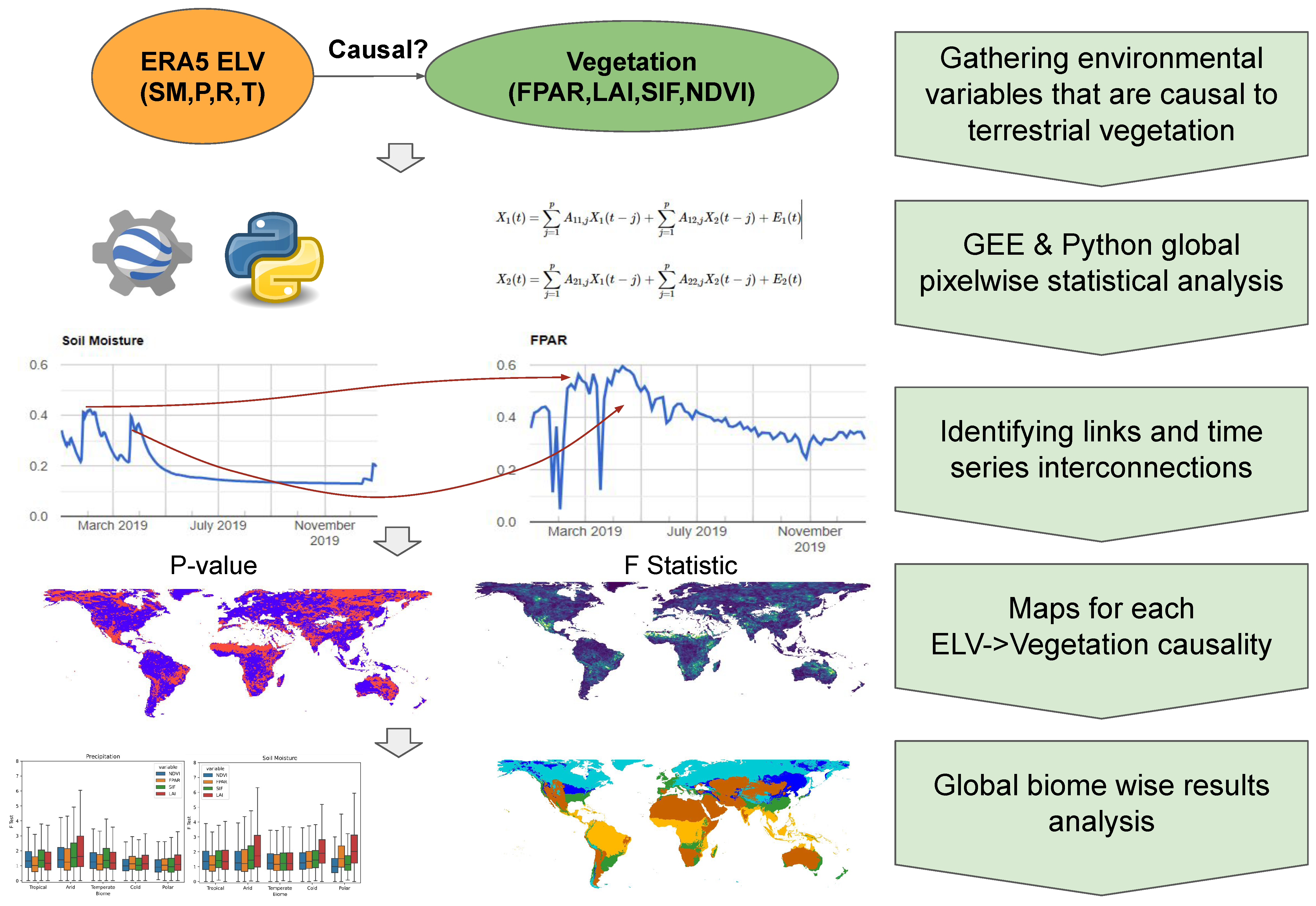
2.1. Granger Causality
2.2. Vegetation Products and Environmental Land Variables
2.3. Global Analysis with Google Earth Engine and Python Geospatial Libraries
2.4. Biome-Specific Analysis
3. Results
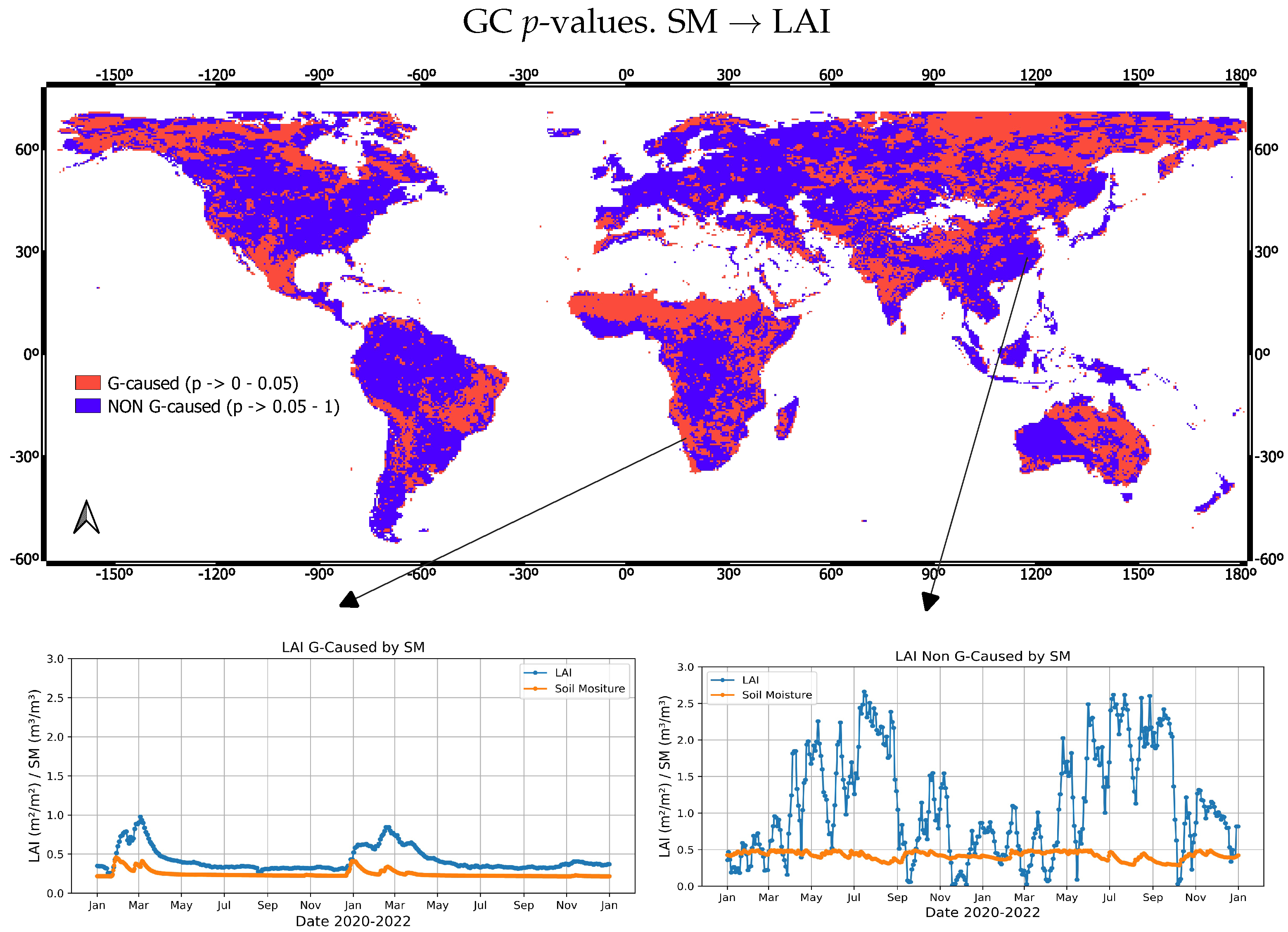
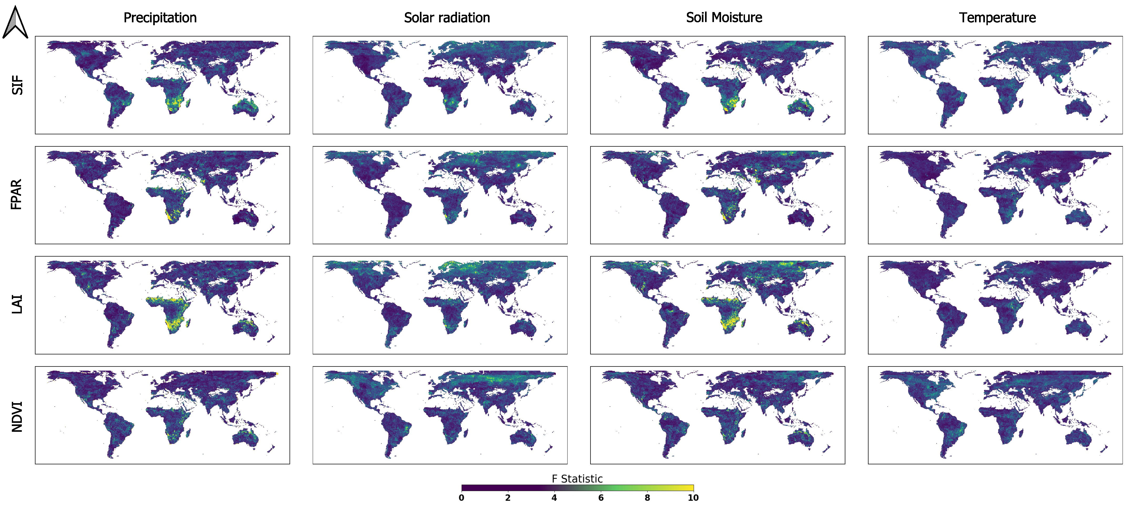
3.1. Global GC Maps
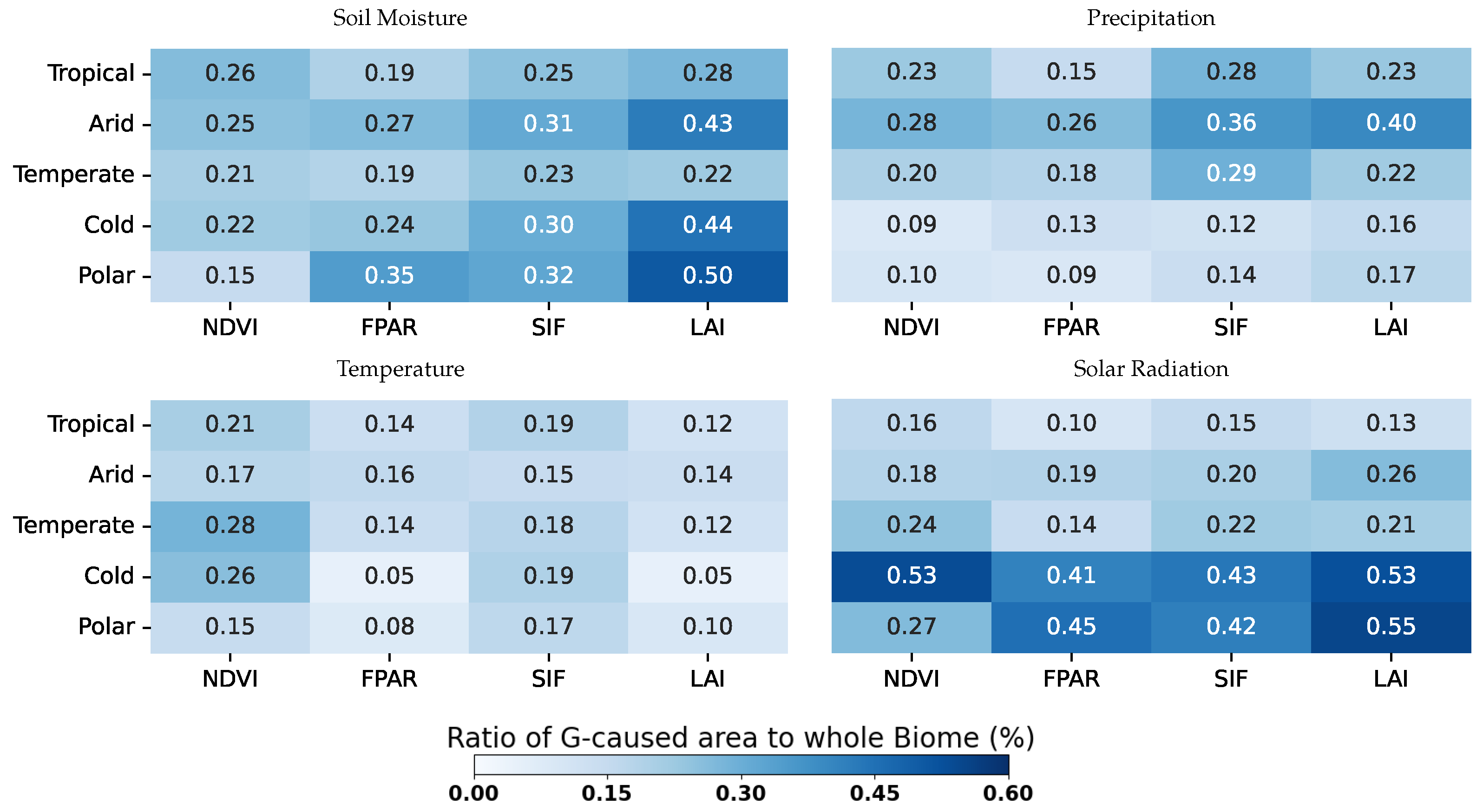
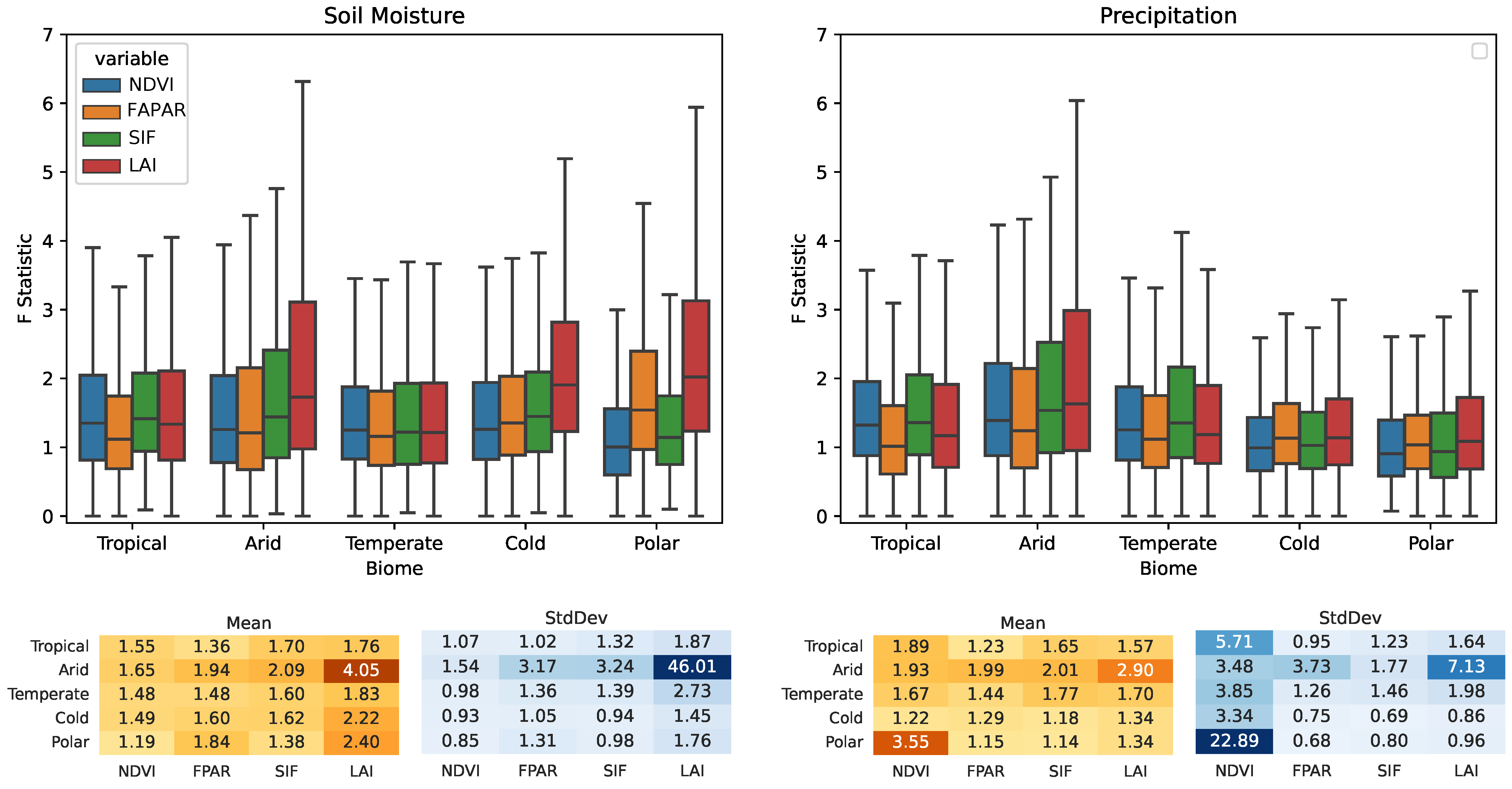
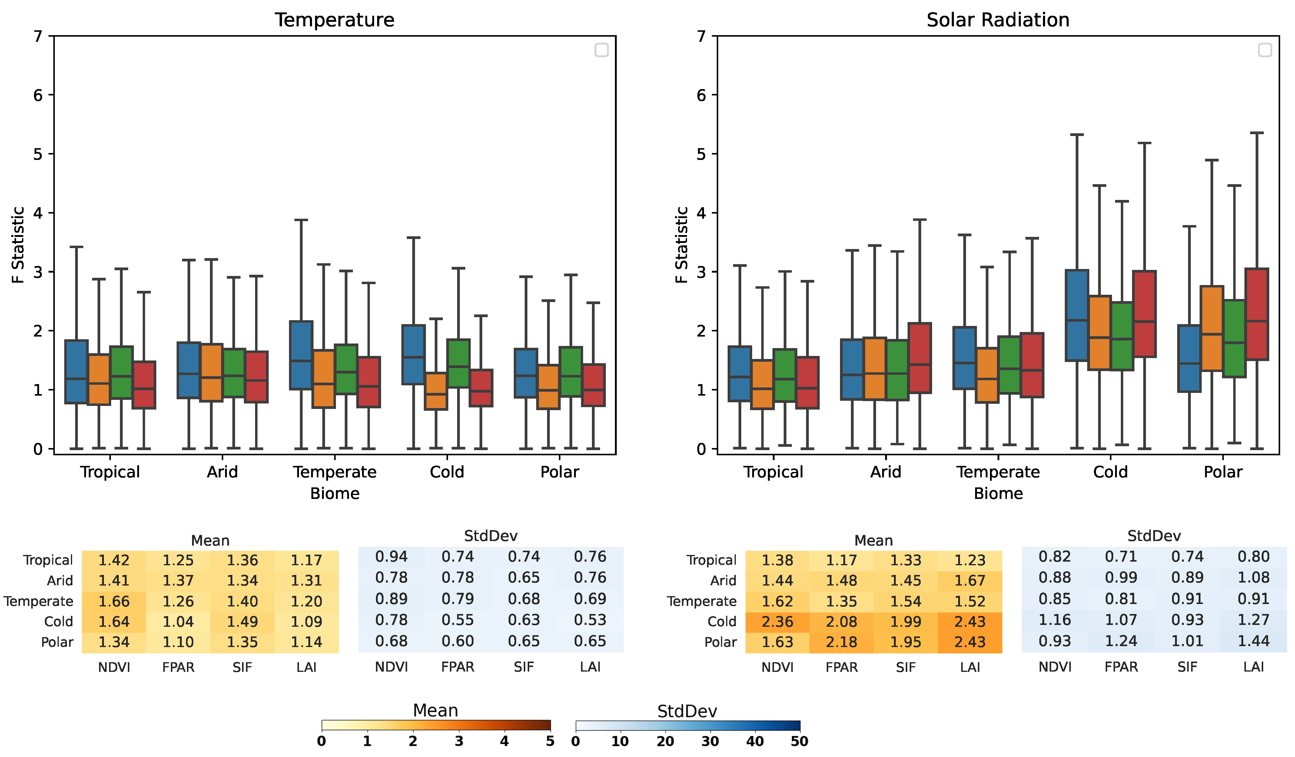
3.2. Köppen–Geiger Biome Specific Analysis
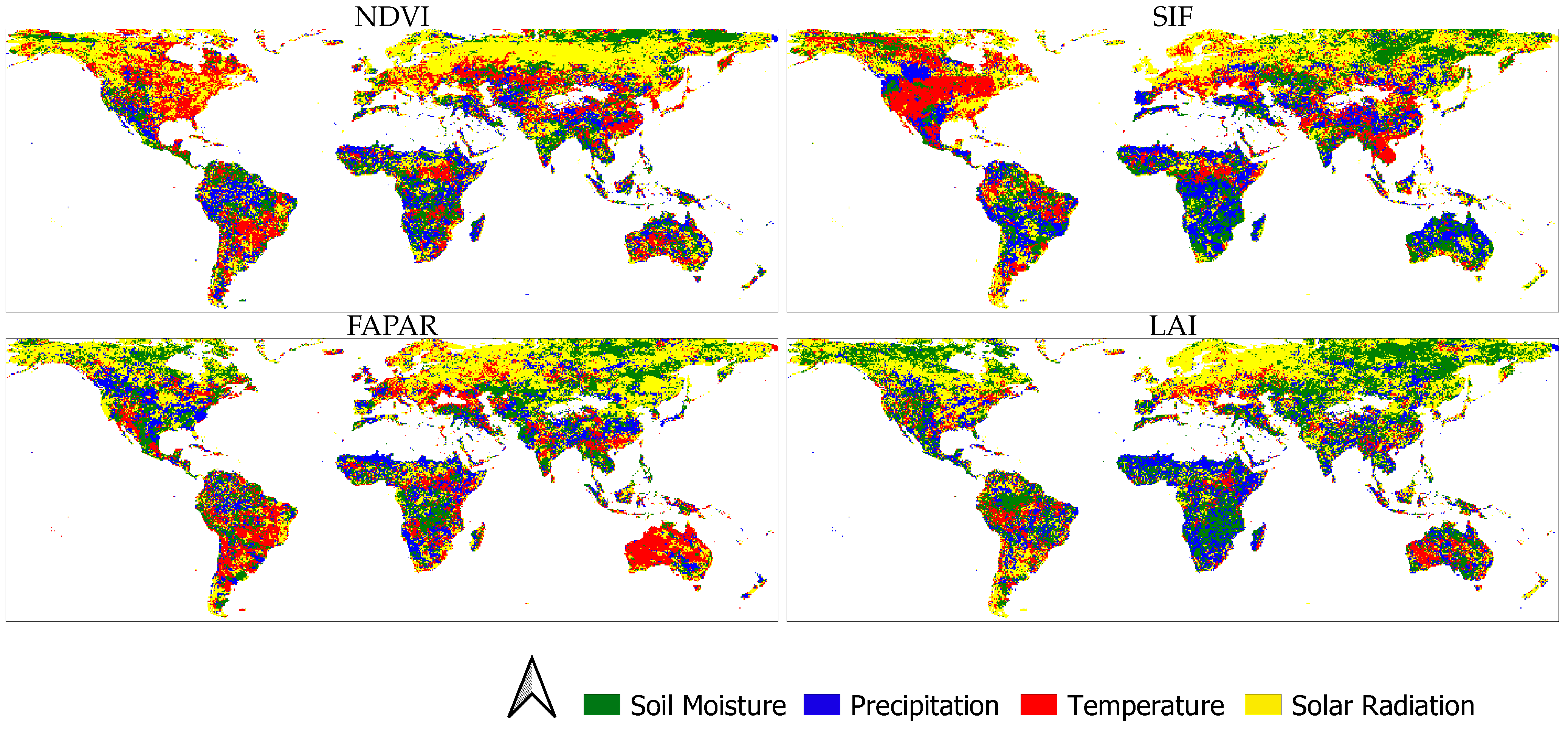
3.3. Main ELV Factors Causing Vegetation Dynamics
4. Discussion
4.1. Water (SM and P)-Caused Vegetation Anomalies
4.2. Energy (T and R)-Caused Vegetation Anomalies
4.3. Limitations and Opportunities for Future Improvements
5. Conclusions
- Water availability (i.e., SM and P) is a strong driver in arid areas, especially for the LAI, which is highly sensitive (0.43 for SM→LAI and 0.41 P→LAI cover a fraction of G-Caused pixel arid biomes).
- SM also causes the LAI on cold and polar biomes with fractions of 0.44 and 0.5, respectively.
- Ecosystems at higher latitudes with cold and polar biomes are driven mainly by R, although R is set to cause the melting of snow, driving soil moisture dynamics. Both on cold and polar biomes, G-Caused areas cover more than 40% of the biomes’ areas.
- T causality is evenly distributed amongst all biomes and VPs, with cover fractions of ∼0.1–0.2.
Author Contributions
Funding
Data Availability Statement
Conflicts of Interest
Appendix A


References
- West, H.; Quinn, N.; Horswell, M. Remote sensing for drought monitoring & impact assessment: Progress, past challenges and future opportunities. Remote Sens. Environ. 2019, 232, 111291. [Google Scholar]
- Breshears, D.D.; Fontaine, J.B.; Ruthrof, K.X.; Field, J.P.; Feng, X.; Burger, J.R.; Law, D.J.; Kala, J.; Hardy, G.E.S.J. Underappreciated plant vulnerabilities to heat waves. New Phytol. 2021, 231, 32–39. [Google Scholar] [CrossRef]
- Mishra, A.K.; Singh, V.P. A review of drought concepts. J. Hydrol. 2010, 391, 202–216. [Google Scholar] [CrossRef]
- Farooq, M.; Hussain, M.; Wahid, A.; Siddique, K.H.M. Drought Stress in Plants: An Overview. In Plant Responses to Drought Stress: From Morphological to Molecular Features; Aroca, R., Ed.; Springer: Berlin/Heidelberg, Germany, 2012; pp. 1–33. [Google Scholar] [CrossRef]
- Qi, Y.; Yu, H.; Fu, Q.; Chen, Q.; Ran, J.; Yang, Z. Future changes in drought frequency due to changes in the mean and shape of the PDSI probability density function under RCP4. 5 scenario. Front. Earth Sci. 2022, 10, 857885. [Google Scholar] [CrossRef]
- Christian, J.I.; Basara, J.B.; Hunt, E.D.; Otkin, J.A.; Furtado, J.C.; Mishra, V.; Xiao, X.; Randall, R.M. Global distribution, trends, and drivers of flash drought occurrence. Nat. Commun. 2021, 12, 6330. [Google Scholar] [CrossRef]
- Fishman, R. More uneven distributions overturn benefits of higher precipitation for crop yields. Environ. Res. Lett. 2016, 11, 024004. [Google Scholar] [CrossRef]
- Dubovyk, O.; Landmann, T.; Dietz, A.; Menz, G. Quantifying the Impacts of Environmental Factors on Vegetation Dynamics over Climatic and Management Gradients of Central Asia. Remote Sens. 2016, 8, 600. [Google Scholar] [CrossRef]
- Berhan, G.; Hill, S.; Tadesse, T.; Atnafu, S. Using satellite images for drought monitoring: A knowledge discovery approach. J. Strateg. Innov. Sustain. 2011, 7, 135–153. [Google Scholar]
- Xu, Y.; Yang, Y.; Chen, X.; Liu, Y. Bibliometric analysis of global NDVI research trends from 1985 to 2021. Remote Sens. 2022, 14, 3967. [Google Scholar] [CrossRef]
- Porcar-Castell, A.; Tyystjärvi, E.; Atherton, J.; Van der Tol, C.; Flexas, J.; Pfündel, E.E.; Moreno, J.; Frankenberg, C.; Berry, J.A. Linking chlorophyll a fluorescence to photosynthesis for remote sensing applications: Mechanisms and challenges. J. Exp. Bot. 2014, 65, 4065–4095. [Google Scholar] [CrossRef]
- Reyes-Muñoz, P.; Pipia, L.; Salinero-Delgado, M.; Belda, S.; Berger, K.; Estévez, J.; Morata, M.; Rivera-Caicedo, J.P.; Verrelst, J. Quantifying Fundamental Vegetation Traits over Europe Using the Sentinel-3 OLCI Catalogue in Google Earth Engine. Remote Sens. 2022, 14, 1347. [Google Scholar] [CrossRef]
- Pinty, B.; Lavergne, T.; Widlowski, J.L.; Gobron, N.; Verstraete, M.M. On the need to observe vegetation canopies in the near-infrared to estimate visible light absorption. Remote Sens. Environ. 2009, 113, 10–23. [Google Scholar] [CrossRef]
- Knorr, W.; Kaminski, T.; Scholze, M.; Gobron, N.; Pinty, B.; Giering, R.; Mathieu, P.P. Carbon cycle data assimilation with a generic phenology model. J. Geophys. Res. Biogeosci. 2010, 115, G04017. [Google Scholar] [CrossRef]
- Weiss, M.; Frederic, B.; Smith, G.; Jonckheere, I.; Coppin, P. Review of methods for in situ leaf area index (LAI) determination: Part II. Estimation of LAI, errors and sampling. Agric. For. Meteorol. 2004, 121, 37–53. [Google Scholar] [CrossRef]
- Kaminski, T.; Knorr, W.; Scholze, M.; Gobron, N.; Pinty, B.; Giering, R.; Mathieu, P.P. Consistent assimilation of MERIS FAPAR and atmospheric CO2 into a terrestrial vegetation model and interactive mission benefit analysis. Biogeosciences 2012, 9, 3173–3184. [Google Scholar] [CrossRef]
- Chen, J.M.; Black, T.A. Defining leaf area index for non-flat leaves. Plant Cell Environ. 1992, 15, 421–429. [Google Scholar] [CrossRef]
- Bréda, N.J.J. Ground-based measurements of leaf area index: A review of methods, instruments and current controversies. J. Exp. Bot. 2003, 54, 2403–2417. [Google Scholar] [CrossRef]
- Seaton, G.G.R.; Walker, D.A. Chlorophyll fluorescence as a measure of photosynthetic carbon assimilation. Proc. R. Soc. Lond. Ser. B Biol. Sci. 1990, 242, 29–35. [Google Scholar]
- Mohammed, G.H.; Colombo, R.; Middleton, E.M.; Rascher, U.; van der Tol, C.; Nedbal, L.; Goulas, Y.; Pérez-Priego, O.; Damm, A.; Meroni, M.; et al. Remote sensing of solar-induced chlorophyll fluorescence (SIF) in vegetation: 50 years of progress. Remote Sens. Environ. 2019, 231, 111177. [Google Scholar] [CrossRef]
- Rouse, W.; Haas, R.; Well, J.; Deering, D.W. Monitoring vegetation systems in the Great Plains with ERTS. Present. Proc. Third Erts Symp. 1974, 1, 309–317. [Google Scholar]
- Myneni, R.B.; Hall, F.G.; Sellers, P.J.; Marshak, A.L. The interpretation of spectral vegetation indexes. IEEE Trans. Geosci. Remote Sens. 1995, 33, 481–486. [Google Scholar] [CrossRef]
- Osakabe, K.; Osakabe, Y. Plant light stress. eLS 2012. [Google Scholar] [CrossRef]
- Bertolino, L.T.; Caine, R.S.; Gray, J.E. Impact of stomatal density and morphology on water-use efficiency in a changing world. Front. Plant Sci. 2019, 10, 225. [Google Scholar] [CrossRef] [PubMed]
- Jones, H.G.; Rotenberg, E. Energy, radiation and temperature regulation in plants. In Encyclopedia of Life Science; John Wiley & Sons, Ltd.: New York, NY, USA, 2001; Volume 8. [Google Scholar]
- Holt, J.S. Plant responses to light: A potential tool for weed management. Weed Sci. 1995, 43, 474–482. [Google Scholar] [CrossRef]
- Markulj Kulundžić, A.; Viljevac Vuletić, M.; Matoša Kočar, M.; Mijić, A.; Varga, I.; Sudarić, A.; Cesar, V.; Lepeduš, H. The combination of increased temperatures and high irradiation causes changes in photosynthetic efficiency. Plants 2021, 10, 2076. [Google Scholar] [CrossRef] [PubMed]
- Moncrieff, G.R.; Hickler, T.; Higgins, S.I. Intercontinental divergence in the climate envelope of major plant biomes. Glob. Ecol. Biogeogr. 2015, 24, 324–334. [Google Scholar] [CrossRef]
- Chen, Z.; Liu, H.; Xu, C.; Wu, X.; Liang, B.; Cao, J.; Chen, D. Modeling vegetation greenness and its climate sensitivity with deep-learning technology. Ecol. Evol. 2021, 11, 7335–7345. [Google Scholar] [CrossRef]
- Bao, G.; Qin, Z.; Bao, Y.; Zhou, Y.; Li, W.; Sanjjav, A. NDVI-based long-term vegetation dynamics and its response to climatic change in the Mongolian Plateau. Remote Sens. 2014, 6, 8337–8358. [Google Scholar] [CrossRef]
- Telesca, L.; Aromando, A.; Faridani, F.; Lovallo, M.; Cardettini, G.; Abate, N.; Papitto, G.; Lasaponara, R. Exploring Long-Term Anomalies in the Vegetation Cover of Peri-Urban Parks Using the Fisher-Shannon Method. Entropy 2022, 24, 1784. [Google Scholar] [CrossRef]
- Olthof, I.; Latifovic, R. Short-term response of arctic vegetation NDVI to temperature anomalies. Int. J. Remote Sens. 2007, 28, 4823–4840. [Google Scholar] [CrossRef]
- Zhang, L.; Qiao, N.; Huang, C.; Wang, S. Monitoring drought effects on vegetation productivity using satellite solar-induced chlorophyll fluorescence. Remote Sens. 2019, 11, 378. [Google Scholar] [CrossRef]
- Papagiannopoulou, C.; Miralles, D.G.; Decubber, S.; Demuzere, M.; Verhoest, N.E.C.; Dorigo, W.A.; Waegeman, W. A non-linear Granger-causality framework to investigate climate–vegetation dynamics. Geosci. Model Dev. 2017, 10, 1945–1960. [Google Scholar] [CrossRef]
- Granger, C.W.J. Investigating Causal Relations by Econometric Models and Cross-Spectral Methods. Econometrica 1969, 37, 424–438. [Google Scholar] [CrossRef]
- Damos, P. Using multivariate cross correlations, Granger causality and graphical models to quantify spatiotemporal synchronization and causality between pest populations. BMC Ecol. 2016, 16, 1–17. [Google Scholar] [CrossRef] [PubMed]
- Maziarz, M. A review of the Granger-causality fallacy. J. Philos. Econ. 2015, 8, 6. [Google Scholar] [CrossRef]
- Friston, K.J.; Bastos, A.M.; Oswal, A.; van Wijk, B.; Richter, C.; Litvak, V. Granger causality revisited. NeuroImage 2014, 101, 796–808. [Google Scholar] [CrossRef] [PubMed]
- Shojaie, A.; Fox, E.B. Granger Causality: A Review and Recent Advances. Annu. Rev. Stat. Its Appl. 2022, 9, 289–319. [Google Scholar] [CrossRef]
- Jiang, B.; Liang, S.; Yuan, W. Observational evidence for impacts of vegetation change on local surface climate over northern China using the Granger causality test. J. Geophys. Res. Biogeosci. 2015, 120, 1–12. [Google Scholar] [CrossRef]
- Reygadas, Y.; Jensen, J.L.; Moisen, G.G.; Currit, N.; Chow, E.T. Assessing the relationship between vegetation greenness and surface temperature through Granger causality and Impulse-Response coefficients: A case study in Mexico. Int. J. Remote Sens. 2020, 41, 3761–3783. [Google Scholar] [CrossRef]
- Rossi, B.; Wang, Y. Vector autoregressive-based Granger causality test in the presence of instabilities. Stata J. 2019, 19, 883–899. [Google Scholar] [CrossRef]
- Li, H.; Huang, F.; Hong, X.; Wang, P. Evaluating Satellite-Observed Ecosystem Function Changes and the Interaction with Drought in Songnen Plain, Northeast China. Remote Sens. 2022, 14, 5887. [Google Scholar] [CrossRef]
- Ozcicek, O.; Douglas Mcmillin, W. Lag length selection in vector autoregressive models: Symmetric and asymmetric lags. Appl. Econ. 1999, 31, 517–524. [Google Scholar] [CrossRef]
- Wismüller, A.; Dsouza, A.M.; Vosoughi, M.A.; Abidin, A. Large-scale nonlinear Granger causality for inferring directed dependence from short multivariate time-series data. Sci. Rep. 2021, 11, 7817. [Google Scholar] [CrossRef]
- Verger, A.; Adrià, D. Copernicus Global Land Operations “Vegetation and Energy”, CGLOPS-1 Algorithm Theoretical Basis Document: Leaf Area Index (LAI), Fraction of Absorbed Photosynthetically Active Radiation (FAPAR), Fraction of green Vegetation Cover (FCover). 2022. Available online: https://land.copernicus.eu/global/sites/cgls.vito.be/files/products/CGLOPS1_ATBD_LAI300m-V1.1_I1.10.pdf (accessed on 28 August 2023).
- Else, S.; Carolien, T. Copernicus Global Land Operations “Vegetation and Energy”, CGLOPS-1 Algorithm Theoretical Basis Document: Normalized Difference Vegetation Index (NDVI). 2022. Available online: https://land.copernicus.eu/global/sites/cgls.vito.be/files/products/CGLOPS1_ATBD_NDVI300m-V2_I1.20.pdf (accessed on 28 August 2023).
- Veefkind, P.; Aben, I.; McMullan, K.; Forster, H.; de Vries, J.; Otter, G.; Claas, J.; Eskes, H.J.; de Haan, J.F.; Kleipool, Q.; et al. TROPOMI on the ESA Sentinel-5 Precursor: A GMES mission for global observations of the atmospheric composition for climate, air quality and ozone layer applications. Remote Sens. Environ. 2012, 120, 70–83. [Google Scholar] [CrossRef]
- Guanter, L.; Bacour, C.; Schneider, A.; Aben, I.; van Kempen, T.A.; Maignan, F.; Retscher, C.; Köhler, P.; Frankenberg, C.; Joiner, J.; et al. The TROPOSIF global sun-induced fluorescence dataset from the Sentinel-5P TROPOMI mission. Earth Syst. Sci. Data 2021, 13, 5423–5440. [Google Scholar] [CrossRef]
- Hersbach, H.; Bell, B.; Berrisford, P.; Hirahara, S.; Horányi, A.; Muñoz-Sabater, J.; Nicolas, J.; Peubey, C.; Radu, R.; Schepers, D.; et al. The ERA5 global reanalysis. Q. J. R. Meteorol. Soc. 2020, 146, 1999–2049. [Google Scholar] [CrossRef]
- Hogan, R. Radiation Quantities in the ECMWF model and MARS. Available online: https://www.ecmwf.int/en/elibrary/80755-radiation-quantities-ecmwf-model-and-mars (accessed on 28 August 2023).
- Muñoz, S.J. ERA5-Land monthly averaged data from 1981 to present. Copernic. Clim. Chang. Serv. (C3S) Clim. Data Store (CDS) 2019. [Google Scholar] [CrossRef]
- Gorelick, N.; Hancher, M.; Dixon, M.; Ilyushchenko, S.; Thau, D.; Moore, R. Google Earth Engine: Planetary-scale geospatial analysis for everyone. Remote Sens. Environ. 2017, 202, 18–27. [Google Scholar] [CrossRef]
- Köppen, W.; Volken, E.; Brönnimann, S. The thermal zones of the earth according to the duration of hot, moderate and cold periods and to the impact of heat on the organic world (Translated from: Die Wärmezonen der Erde, nach der Dauer der heissen, gemässigten und kalten Zeit und nach der Wirkung der Wärme auf die organische Welt betrachtet, Meteorol Z 1884, 1, 215–226). Meteorol. Z. 2011, 20, 351–360. [Google Scholar]
- Beck, H.E.; Zimmermann, N.E.; McVicar, T.R.; Vergopolan, N.; Berg, A.; Wood, E.F. Present and future Köppen-Geiger climate classification maps at 1-km resolution. Sci. Data 2018, 5, 1–12. [Google Scholar] [CrossRef]
- Wu, Y.; Zhang, X.; Fu, Y.; Hao, F.; Yin, G. Response of vegetation to changes in temperature and precipitation at a semi-arid area of Northern China based on multi-statistical methods. Forests 2020, 11, 340. [Google Scholar] [CrossRef]
- Papagiannopoulou, C.; Miralles, D.; Dorigo, W.A.; Verhoest, N.; Depoorter, M.; Waegeman, W. Vegetation anomalies caused by antecedent precipitation in most of the world. Environ. Res. Lett. 2017, 12, 074016. [Google Scholar] [CrossRef]
- Li, W.; Migliavacca, M.; Forkel, M.; Denissen, J.M.; Reichstein, M.; Yang, H.; Duveiller, G.; Weber, U.; Orth, R. Widespread increasing vegetation sensitivity to soil moisture. Nat. Commun. 2022, 13, 3959. [Google Scholar] [CrossRef] [PubMed]
- Zhu, L.; Meng, J. Determining the relative importance of climatic drivers on spring phenology in grassland ecosystems of semi-arid areas. Int. J. Biometeorol. 2015, 59, 237–248. [Google Scholar] [CrossRef]
- Kong, D.; Miao, C.; Duan, Q.; Lei, X.; Li, H. Vegetation-Climate Interactions on the Loess Plateau: A Nonlinear Granger Causality Analysis. J. Geophys. Res. Atmos. 2018, 123, 11–068. [Google Scholar] [CrossRef]
- Snyder, K.; Tartowski, S. Multi-scale temporal variation in water availability: Implications for vegetation dynamics in arid and semi-arid ecosystems. J. Arid. Environ. 2006, 65, 219–234. [Google Scholar] [CrossRef]
- Miranda, J.d.D.; Armas, C.; Padilla, F.; Pugnaire, F. Climatic change and rainfall patterns: Effects on semi-arid plant communities of the Iberian Southeast. J. Arid. Environ. 2011, 75, 1302–1309. [Google Scholar] [CrossRef]
- Post, A.K.; Knapp, A.K. The importance of extreme rainfall events and their timing in a semi-arid grassland. J. Ecol. 2020, 108, 2431–2443. [Google Scholar] [CrossRef]
- Sala, O.E.; Lauenroth, W. Small rainfall events: An ecological role in semiarid regions. Oecologia 1982, 53, 301–304. [Google Scholar] [CrossRef]
- Pietragalla, J.; Pask, A. Stomatal conductance. In Physiological Breeding II: A Field Guide to Wheat Phenotyping; Pask, A., Pietragalla, J., Mullan, D., Reynolds, M., Eds.; CIMMYT: México, Mexico, 2012; pp. 15–17. [Google Scholar]
- Ding, J.; Johnson, E.A.; Martin, Y.E. Optimization of leaf morphology in relation to leaf water status: A theory. Ecol. Evol. 2020, 10, 1510–1525. [Google Scholar] [CrossRef]
- Shi, S.; Wang, P.; Zhang, Y.; Yu, J. Cumulative and time-lag effects of the main climate factors on natural vegetation across Siberia. Ecol. Indic. 2021, 133, 108446. [Google Scholar] [CrossRef]
- Trujillo, E.; Molotch, N.P.; Goulden, M.L.; Kelly, A.E.; Bales, R.C. Elevation-dependent influence of snow accumulation on forest greening. Nat. Geosci. 2012, 5, 705–709. [Google Scholar] [CrossRef]
- Hu, J.; Moore, D.J.; Burns, S.P.; Monson, R.K. Longer growing seasons lead to less carbon sequestration by a subalpine forest. Glob. Chang. Biol. 2010, 16, 771–783. [Google Scholar] [CrossRef]
- Grippa, M.; Kergoat, L.; Le Toan, T.; Mognard, N.; Delbart, N.; L’Hermitte, J.; Vicente-Serrano, S. The impact of snow depth and snowmelt on the vegetation variability over central Siberia. Geophys. Res. Lett. 2005, 32. [Google Scholar] [CrossRef]
- Dye, D.G.; Tucker, C.J. Seasonality and trends of snow-cover, vegetation index, and temperature in northern Eurasia. Geophys. Res. Lett. 2003, 30, 1405. [Google Scholar] [CrossRef]
- Shabanov, N.V.; Zhou, L.; Knyazikhin, Y.; Myneni, R.B.; Tucker, C.J. Analysis of interannual changes in northern vegetation activity observed in AVHRR data from 1981 to 1994. IEEE Trans. Geosci. Remote Sens. 2002, 40, 115–130. [Google Scholar] [CrossRef]
- Austin, A.T.; Yahdjian, L.; Stark, J.M.; Belnap, J.; Porporato, A.; Norton, U.; Ravetta, D.A.; Schaeffer, S.M. Water pulses and biogeochemical cycles in arid and semiarid ecosystems. Oecologia 2004, 141, 221–235. [Google Scholar] [CrossRef]
- Green, J.K.; Konings, A.G.; Alemohammad, S.H.; Berry, J.; Entekhabi, D.; Kolassa, J.; Lee, J.E.; Gentine, P. Regionally strong feedbacks between the atmosphere and terrestrial biosphere. Nat. Geosci. 2017, 10, 410–414. [Google Scholar] [CrossRef]
- Warren, S.G. Optical properties of ice and snow. Philos. Trans. R. Soc. 2019, 377, 20180161. [Google Scholar] [CrossRef]
- Dong, C. Remote sensing, hydrological modeling and in situ observations in snow cover research: A review. J. Hydrol. 2018, 561, 573–583. [Google Scholar] [CrossRef]
- Linacre, E. Climate Data and Resources: A Reference and Guide; Routledge: New York, NY, USA, 2003. [Google Scholar]
- Zuzel, J.F.; Cox, L.M. Relative importance of meteorological variables in snowmelt. Water Resour. Res. 1975, 11, 174–176. [Google Scholar] [CrossRef]
- Marcolla, B.; Migliavacca, M.; Rödenbeck, C.; Cescatti, A. Patterns and trends of the dominant environmental controls of net biome productivity. Biogeosciences 2020, 17, 2365–2379. [Google Scholar] [CrossRef]
- Collow, A.B.M.; Miller, M.A.; Trabachino, L.C. Cloudiness over the Amazon rainforest: Meteorology and thermodynamics. J. Geophys. Res. Atmos. 2016, 121, 7990–8005. [Google Scholar] [CrossRef]
- Nemani, R.R.; Keeling, C.D.; Hashimoto, H.; Jolly, W.M.; Piper, S.C.; Tucker, C.J.; Myneni, R.B.; Running, S.W. Climate-driven increases in global terrestrial net primary production from 1982 to 1999. Science 2003, 300, 1560–1563. [Google Scholar] [CrossRef] [PubMed]
- Kovács, D.D.; Reyes-Muñoz, P.; Salinero-Delgado, M.; Mészáros, V.I.; Berger, K.; Verrelst, J. Cloud-Free Global Maps of Essential Vegetation Traits Processed from the TOA Sentinel-3 Catalogue in Google Earth Engine. Remote Sens. 2023, 15, 3404. [Google Scholar] [CrossRef]
- Hutyra, L.R.; Munger, J.W.; Saleska, S.R.; Gottlieb, E.; Daube, B.C.; Dunn, A.L.; Amaral, D.F.; de Camargo, P.B.; Wofsy, S.C. Seasonal controls on the exchange of carbon and water in an Amazonian rain forest. J. Geophys. Res. Biogeosci. 2007, 112, G03008. [Google Scholar] [CrossRef]
- Chmielewski, F.M.; Rötzer, T. Annual and spatial variability of the beginning of growing season in Europe in relation to air temperature changes. Clim. Res. 2002, 19, 257–264. [Google Scholar] [CrossRef]
- Menzel, A.; Fabian, P. Growing season extended in Europe. Nature 1999, 397, 659. [Google Scholar] [CrossRef]
- Bao, Z.; Zhang, J.; Wang, G.; Guan, T.; Jin, J.; Liu, Y.; Li, M.; Ma, T. The sensitivity of vegetation cover to climate change in multiple climatic zones using machine learning algorithms. Ecol. Indic. 2021, 124, 107443. [Google Scholar] [CrossRef]
- Whetten, A.B.; Demler, H.J. Detection of Multidecadal Changes in Vegetation Dynamics and Association with Intra-Annual Climate Variability in the Columbia River Basin. Remote Sens. 2022, 14, 569. [Google Scholar] [CrossRef]
- Xian, G.Z.; Loveland, T.; Munson, S.M.; Vogelmann, J.E.; Zeng, X.; Homer, C.J. Climate sensitivity to decadal land cover and land use change across the conterminous United States. Glob. Planet. Chang. 2020, 192, 103262. [Google Scholar] [CrossRef]
- Meroni, M.; Rossini, M.; Guanter, L.; Alonso, L.; Rascher, U.; Colombo, R.; Moreno, J. Remote sensing of solar-induced chlorophyll fluorescence: Review of methods and applications. Remote Sens. Environ. 2009, 113, 2037–2051. [Google Scholar] [CrossRef]
- Liu, X.; Liu, L.; Bacour, C.; Guanter, L.; Chen, J.; Ma, Y.; Chen, R.; Du, S. A simple approach to enhance the TROPOMI solar-induced chlorophyll fluorescence product by combining with canopy reflected radiation at near-infrared band. Remote Sens. Environ. 2023, 284, 113341. [Google Scholar] [CrossRef]
- Spracklen, D.; Baker, J.; Garcia-Carreras, L.; Marsham, J. The effects of tropical vegetation on rainfall. Annu. Rev. Environ. Resour. 2018, 43, 193–218. [Google Scholar] [CrossRef]
- Ni, J.; Cheng, Y.; Wang, Q.; Ng, C.W.W.; Garg, A. Effects of vegetation on soil temperature and water content: Field monitoring and numerical modelling. J. Hydrol. 2019, 571, 494–502. [Google Scholar] [CrossRef]
- Chen, Y.; Rangarajan, G.; Feng, J.; Ding, M. Analyzing multiple nonlinear time series with extended Granger causality. Phys. Lett. A 2004, 324, 26–35. [Google Scholar] [CrossRef]
- Gupta, V.; Jain, M.K. Unravelling the teleconnections between ENSO and dry/wet conditions over India using nonlinear Granger causality. Atmos. Res. 2021, 247, 105168. [Google Scholar] [CrossRef]
- Zhong, Z.; He, B.; Wang, Y.P.; Chen, H.W.; Chen, D.; Fu, Y.H.; Chen, Y.; Guo, L.; Deng, Y.; Huang, L.; et al. Disentangling the effects of vapor pressure deficit on northern terrestrial vegetation productivity. Sci. Adv. 2023, 9, eadf3166. [Google Scholar] [CrossRef]
- Pasini, A.; Lorè, M.; Ameli, F. Neural network modelling for the analysis of forcings/temperatures relationships at different scales in the climate system. Ecol. Model. 2006, 191, 58–67. [Google Scholar] [CrossRef]
- Furqan, M.S.; Siyal, M.Y. Random forest Granger causality for detection of effective brain connectivity using high-dimensional data. J. Integr. Neurosci. 2016, 15, 55–66. [Google Scholar] [CrossRef]
- Drusch, M.; Moreno, J.F.; del Bello, U.; Franco, R.; Goulas, Y.; Huth, A.; Kraft, S.; Middleton, E.M.; Miglietta, F.; Mohammed, G.H.; et al. The FLuorescence EXplorer Mission Concept—ESA’s Earth Explorer 8. IEEE Trans. Geosci. Remote Sens. 2017, 55, 1273–1284. [Google Scholar] [CrossRef]
- Van Wittenberghe, S.; Sabater, N.; Cendrero-Mateo, M.; Tenjo, C.; Moncholi, A.; Alonso, L.; Moreno, J. Towards the quantitative and physically-based interpretation of solar-induced vegetation fluorescence retrieved from global imaging. Photosynthetica 2021, 59, 438–457. [Google Scholar] [CrossRef]


| Analysis Product | Spatial Resolution | Temporal Granularity | Algorithm/Retrieval Approach | Sensor | Unit |
|---|---|---|---|---|---|
| LAI/FAPAR | 300 m | 10 Day | Neural networks trained with reflectance data | S-3 OLCI /PROBA-V | LAI: (m2/m2)/FAPAR: (−) |
| NDVI | 300 m | 10 Day | BRDF-normalized, atmospherically corrected reflectances Further corrections for Sun-sensor geometry differences | S-3 OLCI /PROBA-V | (−) |
| TROPOMI SIF(TROPOSIF) | 7 × 3.5 km | Daily | Infilling of Fraunhofer lines at 743–758 and 735–758 nm with fluorescence radiance | S5P | mW m sr |
| Surface Variable | Definition | Unit |
|---|---|---|
| Soil Moisture (SM) | Volume of water in soil layer 2 (7–28 cm) of the ECMWF Integrated Forecasting System. | 1 (volume fraction) |
| Precipitation (P) | Total daily precipitation sum. Accumulated liquid and frozen water, including rain and snow, that falls to the Earth’s surface. | meter (m) |
| Temperature (T) | Temperature of air at 2 m above the surface. 2 m temperature is calculated by interpolating between the lowest model level and the Earth’s surface, taking into account the atmospheric conditions. | Kelvin (K) |
| Shortwave solar radiation (R) | Amount of accumulated shortwave solar radiation (0.2–4 µm direct and diffuse) reaching the surface of the Earth. and the Earth’s surface, taking into account the atmospheric conditions. | J/m |
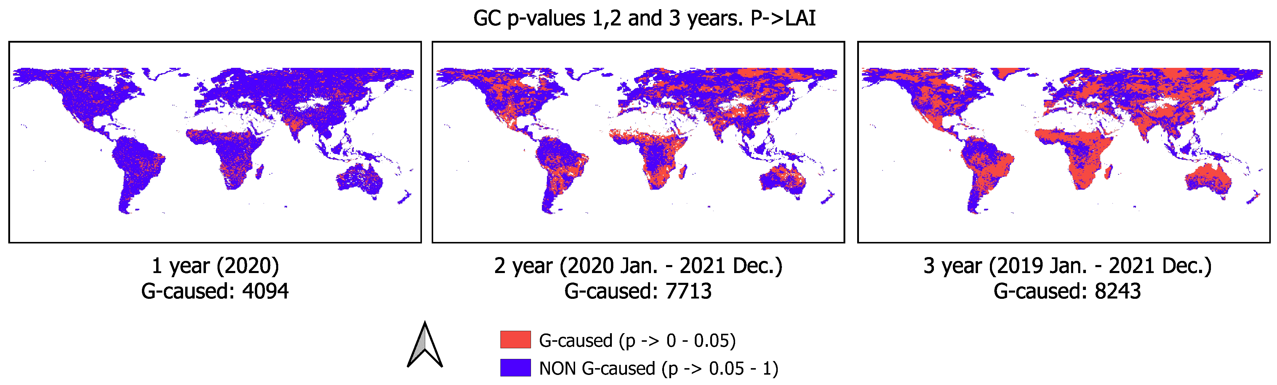
| Time Window | 1 Year | 2 Year | 3 Year |
|---|---|---|---|
| GC significant p-value pixels | 4094 | 7713 | 8243 |
| Increment compared to previous year | - | 88% | 7% |
Disclaimer/Publisher’s Note: The statements, opinions and data contained in all publications are solely those of the individual author(s) and contributor(s) and not of MDPI and/or the editor(s). MDPI and/or the editor(s) disclaim responsibility for any injury to people or property resulting from any ideas, methods, instructions or products referred to in the content. |
© 2023 by the authors. Licensee MDPI, Basel, Switzerland. This article is an open access article distributed under the terms and conditions of the Creative Commons Attribution (CC BY) license (https://creativecommons.org/licenses/by/4.0/).
Share and Cite
Kovács, D.D.; Amin, E.; Berger, K.; Reyes-Muñoz, P.; Verrelst, J. Untangling the Causal Links between Satellite Vegetation Products and Environmental Drivers on a Global Scale by the Granger Causality Method. Remote Sens. 2023, 15, 4956. https://doi.org/10.3390/rs15204956
Kovács DD, Amin E, Berger K, Reyes-Muñoz P, Verrelst J. Untangling the Causal Links between Satellite Vegetation Products and Environmental Drivers on a Global Scale by the Granger Causality Method. Remote Sensing. 2023; 15(20):4956. https://doi.org/10.3390/rs15204956
Chicago/Turabian StyleKovács, Dávid D., Eatidal Amin, Katja Berger, Pablo Reyes-Muñoz, and Jochem Verrelst. 2023. "Untangling the Causal Links between Satellite Vegetation Products and Environmental Drivers on a Global Scale by the Granger Causality Method" Remote Sensing 15, no. 20: 4956. https://doi.org/10.3390/rs15204956