
MosReformer: Reconstruction and Separation of Multiple Moving Targets for Staggered SAR Imaging

School of Electronics and Information Engineering, Harbin Institute of Technology, No. 92 West Dazhi Street, Harbin 150001, China
*
Author to whom correspondence should be addressed.
Remote Sens. 2023, 15(20), 4911; https://doi.org/10.3390/rs15204911
Submission received: 16 August 2023
/
Revised: 4 October 2023
/
Accepted: 5 October 2023
/
Published: 11 October 2023
(This article belongs to the Special Issue Advances in Radar Imaging with Deep Learning Algorithms)
Abstract
:Maritime moving target imaging using synthetic aperture radar (SAR) demands high resolution and wide swath (HRWS). Using the variable pulse repetition interval (PRI), staggered SAR can achieve seamless HRWS imaging. The reconstruction should be performed since the variable PRI causes echo pulse loss and nonuniformly sampled signals in azimuth, both of which result in spectrum aliasing. The existing reconstruction methods are designed for stationary scenes and have achieved impressive results. However, for moving targets, these methods inevitably introduce reconstruction errors. The target motion coupled with non-uniform sampling aggravates the spectral aliasing and degrades the reconstruction performance. This phenomenon becomes more severe, particularly in scenes involving multiple moving targets, since the distinct motion parameter has its unique effect on spectrum aliasing, resulting in the overlapping of various aliasing effects. Consequently, it becomes difficult to reconstruct and separate the echoes of the multiple moving targets with high precision in staggered mode. To this end, motivated by deep learning, this paper proposes a novel Transformer-based algorithm to image multiple moving targets in a staggered SAR system. The reconstruction and the separation of the multiple moving targets are achieved through a proposed network named MosReFormer (Multiple moving target separation and reconstruction Transformer). Adopting a gated single-head Transformer network with convolution-augmented joint self-attention, the proposed MosReFormer network can mitigate the reconstruction errors and separate the signals of multiple moving targets simultaneously. Simulations and experiments on raw data show that the reconstructed and separated results are close to ideal imaging results which are sampled uniformly in azimuth with constant PRI, verifying the feasibility and effectiveness of the proposed algorithm.
1. Introduction
Maritime surveillance is essential for many specific applications, including fishery control, vessel traffic management, accident and disaster response, search and rescue, and trade and economic interests, especially for the surveillance of the Exclusive Economic Zone (EEZ). A spaceborne synthetic aperture radar (SAR) system combined with an automatic identification system (AIS) can offer valuable information to the vessel traffic service (VTS), so as to provide monitoring and navigational advice. A number of studies have demonstrated the capability of traditional SAR systems to detect and image maritime targets. The upcoming generation of spaceborne synthetic aperture radar (SAR) calls for high resolution and wide swath (HRWS). HRWS SAR systems are admirably suited for maritime surveillance applications, offering all-weather and all-day advantages [1,2]. High-resolution images provide reliable information for the identification, confirmation, and description of maritime targets, especially for small vessels. Wide swath coverage, characterized by high temporal resolution with a short revisit time, allows for capturing and tracking dynamic changes in maritime regions [3,4]. Given that SAR was initially developed for the imaging of stationary scenes, the presence of moving targets within an SAR image will result in both spatial displacement and defocusing due to their motion during the SAR integration time. The radial velocity dislocates the target position in azimuth. The along-track velocity causes azimuth blur [5,6]. Furthermore, imaging multiple moving targets becomes challenging, especially when the targets are located in close proximity, causing defocused and overlapping images [7].
In recent years, an increasing number of innovative HRWS SAR systems have been proposed, primarily focused on stationary scenes [8,9,10]. The imaging capability for moving targets remains constrained. A system with the capabilities of ground moving target indication (GMTI) and HRWS imaging uses multiple receive RX channels arranged along the azimuth [11,12]. The multiple channels resolve the inherent trade-off between the low pulse repetition frequency (PRF) and high resolution in HRWS SAR systems. The multiple channels in azimuth increase the spatial degree of freedom, allowing for moving target imaging. However, despite the apparent similarity of multiple channels in HRWS SAR and GMTI systems from a system perspective, they typically need to operate with distinct pulse repetition frequencies (PRFs) to meet their respective performance requirements. As the analysis conducted by [13] shows, the HRWS SAR system operates with , while for the multichannel GMTI system, the PRF should be multiplied by the channel number. Thus, scholars tend to choose a low PRF to guarantee a wide swath and subsequently reconstruct the moving target signals using the low . However, this approach comes with the drawbacks of exaggerating the azimuth ambiguities, along with a long antenna and the expense of high system complexity.
Without the necessity to extend the antenna length, an interesting alternative to multiple azimuth channel HRWS SAR is staggered SAR. It was initially introduced in [14], and subsequent research in [15] further established its principles, attracting widespread attention. It has become the fundamental acquisition mode for satellite systems such as Tandem-L [16,17] and NISAR [18], allowing for seamless ultrawide swath coverage. Since the radar is unable to receive signals during its transmission, there are constant blind ranges across the swath in conventional multiple elevation beam (MEB) HRWS SAR systems [19]. Operated with a variable pulse repetition interval (PRI), staggered SAR shifts these constant blind ranges and redistributes them over the entire swath. Simultaneously, a variable PRI sequence causes the raw data to be sampled non-uniformly with intermittent gaps [20].
Therefore, various reconstruction methods have been proposed to recover the lost data and resample the non-uniform sampling onto a uniformly spaced grid. The simplest way is two-point linear interpolation [21] with a small computational cost. The multichannel reconstruction (MCR) method [22] considers the variable PRIs as multiple apertures and obtains the equivalent uniformly sampled signal using post filters. The authors of [23] modify the MCR method to improve the azimuth ambiguity-to-signal ratio (AASR). The main limitation is that the reconstruction becomes unfeasible when the number of variable PRIs is large. The best linear unbiased interpolation [22] employs the power spectral density (PSD), which can be completed before range compression. The advantage is that the lost data width is only half that of the transmitted pulse duration. These methods are suitable under high oversampling factors. However, the high PRF will deteriorate the range ambiguity-to-signal ratio (RASR) and increase the burden on data volume. To address this issue, an increasing number of techniques have been proposed to reconstruct the images with high precision under medium and low oversampling factors, which includes the iterative adaptive approach (MIAA) [24], nonuniform fast Fourier transform (NUFFT) [25], compressed sensing based on Sparsity Bayesian [26], linear Bayesian prediction (LBP) [27], and so on.
These existing algorithms can precisely reconstruct the images of stationary scenes. However, their performance for moving targets is limited. The BLU reconstruction method uses the power spectrum density (PSD) in the case of a stationary scene. The MCR method is achieved by splicing the Doppler frequency. Since the non-cooperative moving target shifts and extends the Doppler frequency, the reconstruction performance is degraded significantly. Overall, there are two main challenges for imaging moving targets in staggered mode. One is that the non-uniform sampling coupled with the target motion causes reconstruction errors and degrades the reconstruction performance. Specifically, the radial velocity of the target shifts the Doppler center, aggravating the spectrum aliasing induced by non-uniform sampling. The along-track velocity and radial acceleration determine the Doppler chirp rate, which cannot be estimated accurately because of the reconstruction error. These issues increase the azimuth ambiguities, which manifest as artifacts and high sidelobes in azimuth. As a result, these artifacts degrade the imaging performance significantly and potentially lead to misleading interpretations of SAR images since the targets are copied at false positions and obscure the underlying stationary scene. The other challenge is that when dealing with multiple moving targets in the same azimuth, the distinct motion of each target contributes to individualized reconstruction errors. These errors cumulatively aggregate, exacerbating the degradation in imaging performance. As the moving targets are often non-cooperative, it is difficult to obtain the motion parameters as prior information, which is the main obstacle for moving target reconstruction in staggered SAR.
In addition, apart from the reconstruction algorithm for moving targets in staggered SAR, multiple moving target separation is another key issue. The ultra-wide swath offered by staggered SAR usually contains multiple moving targets in azimuth, especially in maritime applications [28]. The simultaneous imaging of multiple moving targets with distinct motion parameters presents a formidable challenge. Particularly when these targets move with similar velocities and are in close proximity, it tends to cause defocused and overlapping images. The multiple moving target imaging methods in the traditional SAR system can be classified into two types: the approach based on the image domain [29,30] and the approach based on the echo data domain [31,32]. The typical methods based on the image domain are hybrid SAR/ISAR [33,34,35] and deep learning techniques [36,37,38]. Both of them compensate for the satellite movement using SAR processing and obtain blurred SAR images. Hybrid SAR/ISAR converts these SAR images into the echo domain and applies ISAR processing to refocus the multiple moving targets, respectively. Deep learning based on a convolutional neural network inputs blurred images and outputs refocused images. These existing algorithms fall short in addressing the challenges associated with moving targets in staggered SAR imaging. This is because these methods only extract the defocused targets’ image (sub-image). However, in staggered mode, the artifacts and ambiguities caused by reconstruction errors tend to spread along the entire azimuth. Extracting the sub-image around the moving target cannot eliminate all the artifacts in the azimuth, degrading the imaging performance more distant from the target. For the approach based on the echo data domain, chirplet transform is used to separate the mixed signal into the signals of each moving target [39]. However, it treats the target as scatterer points and then estimates their motion parameters. The accuracy would be limited in the case of targets with complex structures. Additionally, chirplet transform does not support non-uniform sampling in azimuth, which would not be quite suitable for the staggered mode. So far, little literature can be found in the field of moving target imaging in staggered SAR systems, especially on the reconstruction and the separation of multiple moving targets.
In order to address these challenges, we propose a Transformer-based method to reconstruct and separate the multiple moving targets simultaneously. The task of reconstruction and separation of multiple moving targets in staggered SAR is established. Then, the MosReFormer network architecture is built on the time-domain masking net with an encoder–decoder structure. A gated single-head Transformer architecture with convolutional-augmented joint self-attentions is designed, providing great potential to mitigate the reconstruction error. The loss function of the scale-invariant signal-to-distortion ratio (SI-SDR) is adopted to obtain superior performance. It can improve the imaging performance of multiple moving targets significantly, and the reconstructed and separated results are close to the ideal imaging results, which are sampled uniformly in azimuth with constant PRIs.
Overall, motivated by deep learning techniques, the main contributions of this article are summarized as follows.
- The impact of staggered SAR imaging on moving targets is accessed through temporal and spectral analyses. It becomes evident that the coupling of non-uniform sampling and the target motion result in reconstruction errors and spectrum aliasing, degrading the image quality. These issues need to be addressed effectively.
- We propose a Transformer-based method to image the multiple moving targets in the staggered SAR system. The reconstruction and the separation of the multiple moving targets are solved with a dual-path Transformer. To the best of our knowledge, this is the first article investigating deep learning methods in staggered SAR imaging, and also the first article employing deep learning to address the separation of multiple moving targets within an SAR system.
- The proposed MosReFormer network is designed by adopting a gated single-head Transformer architecture using convolution-augmented joint self-attentions, which can mitigate the reconstruction errors and separate the multiple moving targets simultaneously. The convolutional module provides great potential to mitigate the reconstruction error. The joint local and global self-attention is effective for dealing with the elemental interactions of long-azimuth samplings.
One limitation of our work is the relatively high sensitivity to system parameters. Typically, the PRI sequence is not constant. The system usually presets several sets of PRI sequences for different mission modes on the satellite. In the experiment, we found that the method is sensitive to the PRI values. This also means that the reconstruction and separation performance would be degraded if the test set included parameters of PRI sequences that were not trained. An effective solution is to fully train the several preset sets of PRI sequences, so as to support different PRI sequences. Another limitation is the number of targets. The performance might be compromised when the target number along the azimuth in the scene is large. One potential solution is that combined with sub-aperture technology, multiple targets are divided into blocks and processed separately.
The remainder of this paper is organized as follows. The staggered SAR signal model of moving targets is first described in Section 2. Section 3 analyzes the influence of non-uniform sampling on moving target imaging in the staggered SAR system, illustrating that the coupling of non-uniform sampling and the target motion results in reconstruction errors and spectrum aliasing.
To address this problem, a MosReFormer-based method for staggered SAR moving target imaging is proposed in Section 4, including the task description, preprocessing, the network architecture, and the loss function of the MosReFormer network. In Section 5, simulated data and equivalent raw data have been utilized to verify the feasibility and effectiveness of the proposed method. Section 6 gives a brief conclusion.
2. The Signal Model of Moving Targets in Staggered SAR system
With the technology of multiple elevation beams (MEBs), an HRWS SAR system generates multiple beams directed towards distinct orientations. During transmission, the system illuminates an ultrawide swath as indicated by the broad red beam. On the receiving, digital Beamforming (DBF) is employed to sweep sub-swaths based on the angles of echo arrival. It is also denoted as scan-on-receive (SCORE), as illustrated by the colored regions in Figure 1a. However, since the radar is unable to receive echoes while transmitting, the constant PRI causes constant blind ranges (gaps) in the sub-swaths. Operated with variable PRIs, staggered SAR can address this problem, as shown in Figure 1b. The variable PRIs change the time delays of the echoes and further shift the position of the blind ranges along the azimuth. Consequently, the constant blind areas disappear and instead become distributed across the entire swath, allowing for gapless images.
Staggered SAR employs linear frequency modulation pulses characterized by variable PRIs, denoted as , , and . and represent the maximum and minimum, respectively. The M pulses repeat periodically. The total number of transmitted pulses in slow time is , signifying the sampling number in azimuth. The sth pulse is transmitted at the slow time as
where is the floor operation. The sequence period of the PRI is .
In the staggered SAR geometry for moving targets, the satellite operates at the height H with the speed v along the x-axis. At the initial time, the ith moving target is located at . In the slant range plane, the radial velocity perpendicular to the track is and the velocity along the track is . The radial velocity of the ith target on the ground is , where is the look angle of the radar assuming that v, and are constant during the whole aperture time.
represents the slant range between the ith moving target and the platform at moment. The beam center time is represented as , which corresponds to the moment when the antenna beam reaches the minimum slant range. denotes the motion vectors of the ith target, where is the scattering coefficient, and denotes transpose operation.
The instantaneous slant range between the ith target and the radar is expressed by
The echo pulses are partially or totally lost because the radar cannot receive the signal when it is transmitting. The constant PRI results in constant blind ranges across the whole swath. Operated with the variable PRIs, staggered SAR changes the time delays for the echo pulses. The different transmitted pulses with different PRIs generate different positions of blind ranges, so as to eliminate the constant blind ranges. The blind ranges vary with the slow time, which is represented by the blind range matrix . If the sth echo pulse is lost, the value of the blind matrix equals 0, . Otherwise, . Thus, the echo signal after demodulation can be given as
where represents the fast time, is the antenna pattern weights, and denotes the azimuth envelope. and , denote the wavelength, the pulse duration, and the chirp rate, respectively.
3. The Impact of Staggered SAR Imaging on Moving Targets
In this section, temporal and spectrum analyses are provided to illustrate that the coupling of non-uniform sampling and the target motion results in reconstruction errors and spectrum aliasing. This inevitably deteriorates the imaging performance of multiple moving targets in staggered mode, which can be addressed with the proposed method in Section 4.
3.1. Temporal Analysis
The variable PRIs in staggered SAR cause the pulse losses and the non-uniform sampling in azimuth. Echo pulses that are not lost can be compressed normally in the slant range domain. Thus, we mainly concentrate on analyzing the influence of moving target imaging in azimuth. According to (3), the signal of the ith moving target in azimuth is simplified as
Equation (2) is approximated using a second-order Taylor series expansion, which can be rewitten as
Since we have and , the slant range (5) can be further expressed as
Substituting (3) into (4), the signal sampled non-uniformly in azimuth is given as
where denotes the Doppler center. is the Doppler chirp rate.
The non-uniform sampling can be considered as the sum of a uniform sampling and an offset , as
where is equal to . is the uniform sampling of an ideal reference signal. Based on (7), the ideal reference signal sampled uniformly is expressed as
Therefore, we further explore the relationship between and as follows
The rotation matrixes and . The rotation angle is related to the initial position of the target described by , and is related to the offset . It indicates that the real and imaginary azimuth signal in staggered SAR can be regarded as the reference signal rotated by and in the Re-Im coordinate.
Furthermore, the rotation matrixes ℜ and can be decomposed into two components. One is the terms and , generated by a static target, and the other is the terms and generated by a moving target. It also has , . For the static target, , . In this case, the rotation angles are expressed as and . Thus, the rotation angles caused by moving target are calculated as
It should be noted that the reconstruction algorithms designed for stationary scenes could compensate the terms of and . However, when dealing with moving targets, the non-uniform sampling couples with the target motion will result in reconstruction errors, as shown in and . In particular, for multiple moving targets, the distinct motion of each target contributes to individualized reconstruction errors. These errors degrade the reconstruction performance and increase the azimuth ambiguities, which manifest as artifacts and high sidelobes in azimuth for moving target imaging in staggered SAR.
Spectral Analysis
In order to analyze the spectrum in staggered SAR, the non-uniformly sampled signal is considered as the composite of the M-channel uniform sampled signal. Due to the PRI variation, the completely received M samples within one period can be considered as M channels. Provided that the signal of the reference channel is sampled uniformly by , the signal of the mth channel is given as
In relation to the reference channel, is the time delay of the mth channel. denotes the noise. Thus, the received sampled signal in staggered mode is represented by
Equation (14) can be written in the discrete time domain as
Equation (15) is non-uniform sampling of a continuous time signal, and can be written as
Assuming that , can be rewritten as
where . Owning to the discrete time Fourier transform (DTFT), can also be provided by
Compared (17) with (18), we have
Therefore, the spectrum of the nonuniformly sampled signal is written as
where , , and . The phase term accomplishes time-shifting in the frequency domain. denotes the noise.
Equation (20) illustrates that the spectrum of the nonuniformly sampled signal is the sum of and . denotes the spectrums of the uniformly sampled reference signal. represents the spectrum aliasing due to the non-uniform sampling. The spectrum aliasing aggravates the ambiguities in azimuth.
Figure 2 shows the schematic diagram of the azimuth spectrum in staggered SAR mode. The left sub-figure shows the spectrum for the static target . The yellow lines denote . As apparent from Figure 2, the spectrum aliasing mainly arises from two aspects. One is aliasing from the multiple pairs of uniformly distributed weak caused by non-uniform sampling, as denoted by the blue dotted lines. The other is the spectrum aliasing caused by a non-ideal antenna pattern (sinc-like pattern), as shown with the green dashed line. The shade of gray indicates spectrum aliasing resulting from non-uniform sampling for static targets. When dealing with moving targets, the Doppler center is shifted to . The target motion and the non-uniform sampling are coupled. Consequently, within , the spectrum aliasing caused by the non-uniform sampling is aggravated. Additionally, the spectrum aliasing caused by the non-ideal antenna pattern is also aggravated, as shown in the left of Figure 2. In general, the non-uniform sampling causes spectrum aliasing in azimuth. The non-uniform sampling coupled with the target motion aggravates the spectrum aliasing. This will cause inevitable ambiguities in azimuth.
4. The Staggered SAR Imaging of Multiple Moving Targets Based on the Proposed MosReFormer Network
In this section, the task of the reconstruction and separation of multiple moving targets in staggered SAR is established in Section 4.1. Section 4.2, Section 4.3 and Section 4.4 present the preprocessing, the MosReFormer network architecture, and the loss function of the scale-invariant signal-to-distortion ratio (SI-SDR), respectively.
4.1. Task Description
The task of the proposed MosReFormer network is described and analyzed. The procedure of staggered SAR imaging of multiple moving targets based on the MosReFormer network is provided.
The echo signal of moving targets in staggered SAR was given in (3). After range compression, the signal sampled non-uniformly in azimuth can be expressed as
In order to reconstruct and separate the multiple targets in azimuth, we focus on dealing with the azimuth signal (the azimuth line)Thus, assuming that the number of multiple targets is P, the azimuth signal for each range cell after the range migration correction in staggered mode is written by
where is the amplitude. The nth target has scatterers. is the blind range matrix that describes the data loss for each range cell.
The ideal reference signal of multiple moving targets in azimuth which is sampled uniformly without gaps can be expressed as
where denotes the amplitude. The slow time sampled uniformly . .
Our task focuses on two key issues: (i) Reconstructing the non-uniformly sampled signal into the ideal reference signal . (ii) Separating the echoes of multiple moving targets in azimuth, which can be modeled as
where denotes the operation of reconstruction and separation.
For the reconstruction, we aim to obtain . However, we have found that it is difficult for the Transformer-based network to learn the mapping from to , and the network generalization ability is greatly reduced. One potential explanation is that the difference between the non-uniform sampling time and the uniform sampling time is too small to the order of microseconds. Consequently, the network’s sensitivity to the reconstruction of non-uniform sampling remains limited.
To solve this problem, we opt to employ a simple interpolation method to roughly reconstruct the uniform samplings as , where denotes the spline interpolation operation. Thus, the task in (24) can be rewritten as . The input of the network is , and the outputs are the reconstructed and separated results . The reconstruction error in will be introduced by the coupling of non-uniform sampling and the target motion, as discussed in Section 3.1. Mitigating these errors can be considered a denoising process. Owning to its proficiency in learning feature patterns, the convolutional module is adopted in the proposed MosReFormer network to mitigate these errors.
The flowchart of the proposed Transformer-based algorithm for multiple moving targets in staggered SAR imaging is provided in Figure 3. The first task is to preprocess the echo signal of multiple moving targets and generate the azimuth lines as the network input. Using the given ideal reference signal, the MosReFormer architecture learns a mapping from the mixture azimuth signal to the separated azimuth signal. The optimal parameters of the MosReFormer network are optimized by minimizing the defined SI-SDR loss function. Subsequently, the trained MosReFormer network is employed to reconstruct and separate the azimuth signal containing multiple moving targets, so as to achieve superior imaging performance in staggered SAR. After estimating the Doppler parameters, each target is refocused via azimuth compression, and the final images are obtained.
4.2. Preprocessing
Preprocessing is utilized to generate a normalized azimuth signal in staggered mode as the network input. The network deals with the azimuth signal for each range cell.
The model of staggered SAR echoes is established with the sequences of variable PRIs. After range compression, the spline interpolation is applied to roughly resample the non-uniform signal onto uniform grids. Note that the effectiveness of the interpolation is limited since there appears to be reconstruction errors caused by the coupling of the non-uniform sampling and the target motion. The error can be mitigated with the proposed reconstruction method based on the MosReFormer network. After that, the azimuth compression is performed as a stationary scene. The initial imaging results can be obtained roughly to realize target detection. After target detection, the azimuth lines containing moving targets are found, and the azimuth signal in the time domain before azimuth compression is extracted for each range cell, as shown in the yellow box of Figure 3.
It should be noted that the amplitude range of would be quite extensive, and the value scale changes across different azimuth lines. The unnormalized input signal easily causes weird behavior of loss function topology and excessively accentuates specific parameter gradients, resulting in inadequate training of the network. Therefore, the magnitudes of the azimuth signal are normalized within the interval via the min–max normalization strategy. Meanwhile, different from monaural speech separation, the separation of the multiple moving targets deals with the complex-valued data. In the reconstruction and separation, preserving phase properties is crucial for subsequent signal processing. Thus, the network input is extended into two dimensions, including the real and the imaginary parts as .
4.3. Architecture of MosReFormer Network
Two main issues should be considered in the establishment of the architecture. One issue is the large number of azimuth samplings. This is because a large Doppler bandwidth is usually used to obtain a high resolution. Long samplings in azimuth (long input sequence) prevent the efficiency of elemental interactions, degrading the model performance. The other is the mitigation of the reconstruction error caused by the coupling of non-uniform sampling and the target motion.
To meet these two issues, inspired by the dual-path Transformer models [40], the MosReFormer model is built on the time-domain masking net, which consists of an encoder–decoder structure and a masking net. In the masking net, a gated single-head Transformer architecture with convolutional-augmented joint self-attentions is designed. The joint local and global self-attention is feasible for dealing with the elemental interactions of long-azimuth samplings. The convolutional module provides great potential to mitigate the reconstruction error.
The encoder; the masking net, i.e., the reconstruction and separation net; and the decoder module are detailed in the following.
4.3.1. Encoder
The encoder module transforms the mixture echoes of multiple moving targets into the respective representations within an intermediate feature space. It is responsible for extracting features and comprises a one-dimensional convolutional layer (Conv1D) followed by an optimal nonlinear function . The input azimuth signal is encoded as
where the output is denoted as . , . The input includes the real part and the imaginary part of . Q is the number of filters. We choose the rectified linear unit (ReLU) as to guarantee non-negative representations. denotes the kernel size and the stride is set to half of the kernel size. Thus, we can obtain .
4.3.2. Estimating the Reconstruction and Separation Masks
The masking net realizes the separation by element-wisely multiplying the input with each target’s masks, as
where the P vectors (masks) , and P represents the number of moving targets in azimuth. ⊗ is the Hadamard product.
To accomplish (26), the output of encoder module is operated via layer normalization, which is suitable for long sequences. Then, positional encoding is carried out to describe the location of each element in the sequence, ensuring that each position is assigned a unique representation. Subsequently, a pointwise convolution is applied, effectively reducing the computational burden. After reshaping, the sequence is directed to multiple MosReFormer blocks for sequential processing. The details of the MosReformer block are introduced at the end of this subsection for the sake of consistency.
The output of MosReformer . After the operations of reshaping and ReLU, the sequence . A pointwise convolution is employed, wherein the filter number is , to expand the sequence’s dimension to . The reshaping transforms the sequence from to . and are generated by dual pointwise convolutions. The gated linear unit (GLU) [41] is used as follows:
where denotes the sigmoid function. The GLU output is fed into another pointwise convolution, and, subsequently, it undergoes an ReLU activation function. After that, the output of the masking net is obtained. The representation of the echo signal of each moving target is separated.
4.3.3. Decoder
The decoder module reconstructs the signal from the representation of masking as
where denotes a 1D transposed convolutional layer. represents the reconstruction and the separation of the multiple moving targets’ echoes.
4.3.4. MosReformer Operation
The MosReformer block comprises the convolution modules, a Rotary Position Embedding (RoPE) module, a joint local and global single-head self-attention, and gated units, as shown in Figure 4. The MosReformer block is established based on a gated attention unit (GAU), which combines attention and GLU. The GAU-based module presents advantages in handling long sequences. It uses a simpler single-head attention mechanism with minimal degradation in quality. The convolution module is applied to learn local feature patterns, so as to further mitigate the reconstruction error. The RoPE module encodes the relative position of sequences to obtain the queries, the keys for attention. The joint local and global single-head self-attention allows the model to directly capture elemental interactions across the entire sequence, thus augmenting the model’s capability. A detailed description of these modules is provided as follows.
Within the convolution module, the sequence is initially normalized and processed through a linear layer. This is followed by a Sigmoid-weighted Linear Unit (SiLU) activation function. Subsequently, it undergoes a 1D depthwise convolution, where each input channel is convolved with a different kernel. Shortcut connections are employed to connect the output and the input of the depthwise convolution layer, allowing for feature reuse and mitigating vanishing gradients. After shaping, the dropout is performed to improve the generation and reduce overfitting. The operation of the convolution module is denoted as .
The RoPE module is combined with per-dim scalars and offsets. We assumed that the output of the convolution module is .
Applying per-dim scalars and offsets to , it can be obtained that . Using RoPE technology [42], the relative position information can be added to and as follows:
where and are the parameters related to the rotary matrix. Using (29), we can obtain the keys and and the queries and . It also provides a method to reduce the size of the attention matrix.
The advantage of RoPE is that it encodes the absolute position with a rotation matrix and, meanwhile, incorporates the explicit relative position dependency in self-attention formulation. The input of the proposed MosReFormer network is the azimuth line of each range cell. The spatial information is obtained via range compression. The position encoding can capture the temporal information of the signal in a certain spatial dimension (the position of the input). It can evaluate the temporal distance of signal samplings. Furthermore, owing to the relative position encoding, the rotary position embedding supports the flexibility of signal length. This feature is vital for reconstructing and separating the moving targets in staggered SAR imaging.
The module of joint local and global single-head self-attention uses a triple-gating process in [40,42]. The input of the attention , is obtained after the convolution module as and . Note that the feature dimensions are expanded from Q to . For long sequences with large T, the size of the attention matrix is , and thus it will be difficult to calculate the attention matrix. The global and local attention can effectively replace the solution of the attention matrix. Using a low-cost linearized form, the global attention can be obtained as
where is the scaling factor. The local attention is obtained by
where . The matrix , , and are divided into H chunks without overlapping. P is the size of each chunk. After concatenating (31), the finial local attentions are shown as and . Thus, the joint attentions can be given as and . After that, the output sequence of MosReformer block can be represented by
where denotes the activation function. The joint attention can directly model the interactions of the long sequences. The MosReformer block repeats several times to obtain the final .
4.4. SI-SDR Loss Function
The network is trained by minimizing a loss function utilizing large datasets. Inspired by the objective measure in [43], the scale-invariant signal-to-distortion ratio (SI-SDR) is adopted. Assume that the output is the azimuth signal of the nth target, , and its estimate is denoted by . The SI-SDR ensures that the residual is orthogonal to , as
Rescaling in a manner that the residual becomes orthogonal to it. It is equvalent to identifying the orthogonal projection of on the line spanned by . Thus, the optimal scaling factor is equal to . The scale reference is defined as . The estimate can be decomposed as , leading to the expanded formula as
It should be noted that the SI-SDR has superior performance in least-squares and the signal-to-noise ratio (SNR) [44]. . It is because that the residual is not guaranteed to be orthogonal to the signal . For instance, in the objective measure of SNR, consider the orthogonal projection of onto the line spanned by . It generates a right-angled triangle with the hypotenuse , i.e., . This also means that the value of SNR is always positive.
5. Experimental Results and Analysis
Section 5.1 provides an overview of the dataset and experimental configuration. In Section 5.2, Section 5.3 and Section 5.4, simulations and experiments on equivalent data in staggered SAR mode are employed to validate the feasibility of the proposed algorithm.
5.1. Dataset and Experimental Configuration
The azimuth signal in staggered mode and the reference azimuth signal are generated as data pairs for MosReFormer network training. The preprocessing is implemented to generate the azimuth signal in the time domain for network input. The reference azimuth signal is generated by an SAR system without blind ranges sampled uniformly. The constant PRI is obtained as . Table 1 lists the simulated parameters of the staggered SAR system. The illuminate duration is commonly much larger than the synthetic aperture duration to observe the azimuth ambiguity caused by the non-ideal antenna pattern. In this paper, the illumination time is 4.5 times . Therefore, the long sampling in azimuth results in a long input sequence, increasing the complexity of the reconstruction and separation tasks. However, this challenge can be addressed effectively with the proposed MosReFormer network.
Even though the network input is the 1D azimuth signal, we simulate a scene block of which the size is 22 km × 2 km to improve the generation efficiency of the data pairs. The scene contains multiple moving targets. The number of moving targets randomly varies between three and six within each scene block. In this paper, the separation of moving targets is referred to as the multiple targets in azimuth. Thus, each scene should ensure more than one moving target along the azimuth for some range cells. The 3D ship models are established using ray tracing. To ensure diversity within the dataset, a variety of vehicle types are simulated as moving targets in the scene, each exhibiting different sizes and characteristics. The amplitudes of scattering coefficients obey the uniform distribution . The along-track velocities , and the radial velocities . The MosReFormer network is trained with 160k training lines and 1k lines are used for testing. The division of the training and testing set ensures randomness. The data division is operated randomly to prevent bias in the data distribution that might affect model evaluation. The test data do not contain information from the training data. Furthermore, the data preprocessing of the training set and the testing set ensures consistency. The input SNR obeys the uniform distribution, .
The training process was performed on a computer equipped with Intel Xeon Silver 4210R 2.40-GHz CPU, 480-GB RAM, and double NVIDIA GeForce RTX 6000 with 48-GB hardware capabilities. The MosReFormer network was implemented with Pytorch 2.0 and CUDA 11.0. Optimization was achieved using the SGD optimizer. The configuration of the training process of the MosReFormer network is given in Table 2. The batch size is set to 10, and seven epochs have been run in the experiment. The learning rate undergoes a gradual warming up for the initial 3k steps, followed by a linear reduction, ultimately diminishing to 0 after 11k steps. The convergence criterion is to run the test set in every 1k training steps and select the checkpoint with the lowest loss value as the final model. For the hyper-parameters, the number of MoReformer blocks is 24 and the dimension of the encoder output Q is 512. The encode kernel size and stride are set to 16 and 8. The depthwise convolution kernel size is 17. The chunk size P is 256 and the attention dimension d is set to 128. The gating activation function is Sigmoid. The training and inference curves are given in Figure 5. The training loss diminishes with an increase in the number of iterations. Meanwhile, the inference loss exhibits a gradual decline, eventually converging to a low value of −25 dB around 110k iterations. A slight discrepancy in performance between the training and validation sets may be attributed to the characteristics of the dataset.
Furthermore, in the sequence of variable PRIs, the PRI strategy has a linear trend as
where denotes the difference between two adjacent pulses. We adopt the fast linear PRI variation strategy in the experiments because two consecutive pulses will not be lost for all slant ranges. In the fast linear PRI sequence, is obtained as
where and , is the floor operation. and denote the maximum and minimum slant ranges, respectively. . M is obtained as [45]
These parameters’ values are given in Table 1. The PRI trend, the location of blind ranges, and the percentage of lost pulses are illustrated in Figure 6. It can be observed that there are no consecutive lost pulses for all slant ranges within the desired swath. The benefit lies in low sidelobes in the vicinity of the main lobe in azimuth.
5.2. Results and Analysis of Multiple Moving Point Targets
To verify the feasibility and effectiveness of the proposed method for multiple moving target imaging in staggered SAR, five moving point targets are simulated. The scene consists of one central target surrounded by four targets in the vicinity. The central target is located at a slant range of 935 km. As the network input is a 1D azimuth signal, it is essential to verify the potential impact of a signal originating from targets located at the same azimuth cell but different slant ranges on the output performance. Thus, the azimuth position and motion parameters of the three bottom targets are set to be identical.
The imaging results of the multiple moving point targets are shown in Figure 7 using different methods, and the zoomed-in versions with a span of 2400 azimuth indexes are provided in Figure 8. Figure 7a,b are the staggered SAR imaging results using the interpolation reconstruction method. The targets in Figure 7a are displaced and defocused. This is because the radial velocities lead to azimuth dislocation and the along-track velocities cause azimuth smearing. After estimating the Doppler center and the Doppler chirp rate , the moving targets are refocused, as shown in Figure 7b. For simplicity, we use DIRIS and IRIS to represent the methods in Figure 7a,b. Even though the interpolation can resample the non-uniform sampling into uniform grids, the coupling of non-uniform sampling and target motion causes reconstruction errors as in (11) and in (12). It results in artifacts and high sidelobes spread along all of the azimuth, aggravating the azimuth ambiguity and degrading the imaging performance significantly. The amplitudes are in logarithmic scale, ranging from −70 dB to 0 dB, so as to better visualize the details of these artifacts.
Figure 7d and Figure 8d illustrate the imaging results of the proposed algorithm based on the MosReFormer network. The artifacts and high sidelobes are obviously suppressed and alleviated in azimuth, not only for the sidelobes in the vicinity of the target but also for the more distant sidelobes. In particular, for the azimuth indexes spanning from 4000 to 10,000, Figure 7a,b have a lot of high sidelobes which are shown as blue spots, while in Figure 7c,d, high sidelobes are primarily distributed around the range of 6500 to 7500. Moreover, the azimuth signal of each range cell can be considered as the superposition of multiple chirp signal components. However, the azimuth signal and the range signal are coupled for SAR processing. The network input signal may be potentially influenced by the range signals originating from targets located at different slant ranges. The results show the robustness of the MosReFormer network when dealing with multiple targets located at different slant ranges.
The reference ideal imaging results with constant PRIs are presented in Figure 7c and Figure 8c. Without the blind ranges and the non-uniform azimuth sampling, the reference results show ideal imaging performance in terms of azimuth ambiguity. It should be noted that the separations we used in Figure 7a–c are also ideal in the simulation. The performance of the separation would be further degraded due to the limited accuracy of the actual separation methods. Simultaneously, the performance of separation achieved by the MosReFormer network closely approaches the ideal performance, thus verifying its feasibility and effectiveness.
To observe more details of the artifacts and sidelobes, the profiles of the azimuth impulse response of the central moving target are provided in Figure 9. As apparent from Figure 9a, the moving target is displaced and defocused because of the target motion. In Figure 9b, even though the target motion is compensated, the coupling of non-uniform and target motion leads to a lot of high sidelobes and artifacts. Typically, within the azimuth distance of −5 km to 5 km, the sidelobes are concentrated at −60 dB to −20 dB. Within the azimuth distance of −3 km to 3 km, the sidelobe exceeds −40 dB and the highest sidelobe reaches approximately −20 dB. As shown in Figure 9c, these artifacts and high sidelobes are notably suppressed using the proposed MosReFormer network. Within the azimuth distance of −2 km to 2 km, the sidelobes are below −60 dB. In the vicinity of the mainlobe, the sidelobes are nearly below −40 dB, which significantly improves the imaging performance. Moreover, it should be noted that a pair of higher sidelobes appears 9.18 km away from the mainlobe, caused by the non-ideal antenna pattern. The antenna power pattern follows sinc-like window rather than rectangular window. In Figure 9, the blue and yellow arrows indicate the highest sidelobes generated by the antenna power pattern and the second-highest sidelobe in their vicinity. The yellow arrow highlights the sidelobe in the reference result. These pairs of sidelobes in the DIRIS, the IRIRS, and the MosReFormer appear slightly lower than those in the reference results.
The integrated sidelobe ratio (ISLR), the entropy, and the peak sidelobe ratio (PSLR) are provided in Table 3 to access the imaging performance quantitatively. The outcomes in Table 3 demonstrate that the proposed algorithm outperforms its competitors in terms of entropy, PSLR, and ISLR. The algorithm’s performance closely resembles the results of the uniform reference, revealing that superior imaging performance is attained.
5.3. Results and Analysis of Simulated SAR Data
Simulated staggered SAR data are utilized and analyzed to further demonstrate the feasibility and effectiveness of the proposed algorithm. In the scene of 22 km km , there are five ship targets with different target motions. For simplicity, the two distant targets on the left are denoted as Target 1 and Target 2. Target 3 is situated in the middle, and Target 4 and Target 5 are located on the right. The scene center is located at the slant range of 950 km. Each target is composed of multiple scattering points. The attitudes and directions of these ships are different to evaluate the method’s robustness.
Figure 10 shows the imaging results of multiple simulated ship targets in staggered mode, and the zoomed-in versions of the five targets are provided in Figure 11. Figure 10a, using DIRIS, illustrates the displaced and defocused imaging results along with a lot of artifacts and high sidelobes. The non-ideal antenna power pattern, the oversampling rate, the non-uniform sampling, and the target motion are the issues causing the azimuth ambiguities. The non-ideal antenna pattern results in high sidelobes at fixed positions away from the targets, specifically at the azimuth indexes around 1500 and 12,500. Compared with the results in staggered mode, the reference result with a constant PRI in Figure 10d has higher sidelobes caused by the ideal antenna pattern. A high oversampling rate can enhance the performance of azimuth ambiguity, but it comes at the expense of an increased range ambiguity-to-signal ratio (RSAR) and the burden of data volume. The target motion mainly leads to displaced and smearing images, increasing the sidelobes in the vicinity of the targets. The non-uniform sampling coupled with the target motion aggravates the artifacts and the spreading of high sidelobes along all of the azimuth. The multiple moving targets with different target motions exacerbate the situation even further.
In Figure 10b, the Doppler parameters are estimated and compensated after interpolation reconstruction. There would be reconstruction error caused by the coupling of non-uniform sampling and motion. Consequently, the targets are replaced and refocused along with a significant number of high sidelobes, leading to azimuth ambiguity and degrading the imaging performance. Moreover, as shown in the zoomed-in versions in the left two columns of Figure 11, the artifacts are aliased onto another actual target, which subsequently affects the image interpretation. Additionally, Figure 10c and Figure 11 provide the imaging results using the Range-Instantaneous-Doppler (RID) method for comparison. The RID method is based on the hybrid SAR/ISAR technique [46], which is designed for refocusing a moving target. SAR processing is to compensate for the movement of the satellite, and ISAR processing is to compensate for the movement of the moving target. Smoothed pseudo Wigner–Ville distribution (SPWVD) is adopted in the RID method, which can deal with the complex motion of targets. The high sidelobes near the targets are suppressed effectively, as shown in the third column of Figure 11. However, the sidelobes away from the targets cannot be suppressed in staggered mode, as shown by the azimuth indexes from 4000 to 8000 in Figure 10c. This is because the hybrid SAR/ISAR method is operated on the image domain, and the sub-image selection limits the scope. Each sub-image we selected only includes the target. Moreover, the displaced position of the image caused by the radial velocity cannot be solved. As a result, the position of the target is displaced, as in Figure 10a.
In general, moving target imaging processing should focus on addressing two main problems: mitigating the reconstruction error to suppress the high sidelobes in azimuth, and separating the echoes of multiple targets accurately to improve the imaging performance. These two problems can be effectively alleviated based on the proposed MosReFormer network. As shown in Figure 10d, the artifacts and the high sidelobes are suppressed along the azimuth. It also indicates that the echoes of multiple moving targets with different attitudes and motion parameters are separated accurately. Meanwhile, as apparent from Figure 11, there is a subtle difference between the zoomed-in results of the MosReFormer network (the last column) and the ideal reference results (the third column). Despite the targets being focused almost identically, there exist minor artifacts dispersed around the targets. Even though the focusing performance of the targets is almost the same, there are some slight artifacts dispersed near the targets. These artifacts stem from the ambiguities introduced by other adjacent targets in azimuth. This becomes more evident when comparing Target 3 in Figure 11c, which has fewer artifacts due to the absence of adjacent targets in azimuth.
In order to intuitively illustrate the effectiveness of the MosReFormer network in reconstruction and separation, the examples of the input azimuth signal, the ideal reference azimuth signal, and the output azimuth signal by the MosReFormer network are provided in Figure 12. Figure 12a shows the azimuth signal of Target 1 and Target 2 at the 70th range index. The amplitude of the input signal, represented by the yellow line, is modulated by the sinc-like antenna pattern. The input signal is the composite of the theoretical azimuth signal of Target 1 and the theoretical azimuth signal of Target 2. In signal processing, the azimuth signal of Target 1 and Target 2 are aliased together and cannot be separated. Direct azimuth compression would result in defocused and displaced images. In the upper right part of the subfigure, the zoomed-in version is given. The pulse loss causes the gaps in the azimuth signal, which can be clearly in the zoomed-in version. The ideal reference azimuth signal of Target 1 and Target 2 is shown in the middle of Figure 12a. The output azimuth signal using the MosReFormer network is illustrated on the right of Figure 12a. The signals of Target 1 and Target 2 are separated, and the gaps are eliminated. Figure 12b shows the azimuth signal of Target 3. The result of MosReFormer is close to the ideal reference, indicating that the MosReFormer network is also well-suited for a single target. The examples of the azimuth signals of Target 5 and Target 6 at the 466th range index are provided in Figure 12c, showing that it is effective for azimuth signals at different slant ranges.
The entropies of the five targets and the entire scene using different methods are provided in Table 4. The value of image entropy can be utilized to quantify the spatial disorder of an image. The SAR images of ship targets that exhibit clearer structures and better-focused scatterers tend to have smaller entropy values. The entropy of an image [47] can be defined by
where g and h denote pixel numbers in the azimuth and slant range. The defocused images using DIRIS have the largest entropies. Although the RID method can refocus moving targets effectively, the high sidelobes along all of the azimuth increase the entropies. The entropies of the MosReFormer are close to those of the ideal reference, and they are much lower than those of the DIRIS and IRIRS methods. This indicates that the MosReFormer network achieves better imaging quality and more accurate target separation, leading to superior focused staggered SAR images of multiple moving targets.
5.4. Experiment on Spaceborne SAR Data
To validate the effectiveness of the reconstruction and the separation, Gaofen-3 data are utilized to generate artificially equivalent data in staggered mode. The real spaceborne data were acquired by the GF-3 satellite over the city of Dalian in China. The large scene is situated along the coastline and comprises hills, villages, a small island, and the sea surface. The echoes of ship targets are simulated using ray tracing and added to the echoes of the spaceborne data. The generation of staggered equivalent data was proposed and analyzed in reference [45]. According to variable PRIs, the uniform signal is sampled using two-point interpolation, and blind ranges are considered after range compression. The reconstruction of the stationary scene is obtained via spline interpolation. The moving targets are detected and processed as in Figure 3. Note that the azimuth signal should be normalized in the preprocessing before inputting the network. To maintain the consistency of the magnitude, the normalized magnitude has to be reversed in the azimuth of each range cell.
The imaging results of the large scene are displayed in Figure 13. The zoomed-in versions of the ship targets of offshore and inshore scenes are provided in Figure 14 and Figure 15, respectively. As apparent from Figure 13a,b, spline interpolation can achieve acceptable performance for a stationary scene. For the moving targets, the image qualities are degraded due to the reconstruction error. The presence of high sidelobes and artifacts aggravates the azimuth ambiguity, leading to an increased probability of false alarms for targets. This adversely affects the accuracy and reliability of target detection in SAR imaging. In Figure 14c and Figure 15c, the RID method can compensate for the movement of the moving target, but the sidelobes along all of the azimuth cannot be suppressed. The moving targets are also displaced due to the radial velocities, and the positions are the same as those in Figure 15a. In Figure 14d and Figure 15d, the proposed MosReFormer network alleviates the error caused by the coupling of non-uniform sampling and the target motion. Additionally, it accurately separates the echoes of multiple moving targets in azimuth, closely resembling ideal separated results. The reference imaging result in Figure 13c has superior imaging performance with a constant PRI and without blind ranges. Even though there is a slight difference between the results of the proposed method and the ideal reference, the artifacts and high sidelobes are significantly suppressed compared with the DIRIS and IRIRS methods.
The imaging results of the inshore scene have the artifacts of the static scene on the coastline, as apparent from the bottom of Figure 15. The proposed algorithm can effectively focus on moving targets in both the inshore scene and the offshore scene and can significantly suppress sidelobes in the azimuth dimension. In the meantime, it can be observed that for the inshore scene, the background clutter is complex and there are artifacts caused by stationary scenes. These factors would have some slight impact on the separation and reconstruction of echoes. In order to provide more details about including both inshore and offshore scenes to compare the effectiveness of the methods, the zoomed-in versions of the moving target in the bottom right of Figure 14 and the moving target in the bottom left of Figure 15 are shown in Figure 16. The entropies of the imaging results using different methods are also provided in Table 5. The proposed MosReFormer network has smaller entropies compared with its rivals. This demonstrates the method’s robustness and capability in the reconstruction and separation of multiple moving targets in staggered SAR mode.
6. Conclusions
In this article, we verify the feasibility of employing deep learning to moving target imaging in staggered SAR and propose the MosReFormer network to reconstruct and separate the multiple moving targets simultaneously. The proposed MosReFormer framework employs a convolutional encoder–decoder structure to mitigate the reconstruction error caused by the coupling of the non-uniform sampling and the target motion. The joint local and global self-attention are utilized to deal with the elemental interactions of long-azimuth samplings. The SI-SDR loss function is defined to ensure the performance of the MosReFormer network. Compared with other algorithms, the artifacts and high sidelobes can be suppressed, leading to significant alleviation of ambiguities in azimuth. The echoes of multiple moving targets in azimuth can be separated in the time domain. Consequently, the reconstruction error can be mitigated, and the multiple moving targets can be accurately refocused and imaged. Simulations and experiments on equivalent GF-3 data in the staggered SAR system verify the reliability of the proposed imaging method for multiple moving targets based on the MosReFormer network.
One potential future extension of our work is to modify the MosReFormer network to adapt to moving targets with complex motion patterns, especially maritime targets with 3D rotation. In this case, the echo signal in staggered mode is no longer in the form of linear frequency modulation, but a translational component of higher order and its own rotation component, along with non-uniform sampling. Conventional SAR technology can attain precise compensation for higher-order translational terms, yet its influence on rotational components remains limited. The MosReFormer network is conceived upon the architecture employed in source separation and speech enhancement, thereby endowing it with the capacity for generalization to deal with complex signal forms. Furthermore, the current method supports the elaborated linear PRI sequence. In future work, the robustness can be enhanced to align with diverse PRI variation strategies. Additionally, we plan to incorporate the detection of moving targets into the MosReFormer architecture, aiming to achieve the integration of detection, separation, and refocusing of multiple moving targets in staggered SAR.
Author Contributions
Conceptualization and methodology, X.Q. and Y.Z.; writing—original draft preparation, X.Q.; writing—review and editing, X.Q., Y.Z. and Z.L.; supervision, Y.J. and C.Y. All authors have read and agreed to the published version of the manuscript.
Funding
This work was supported in part by the National Natural Science Foundation of China under Grant 61971163 and Grant 61201308, and Youth Science Foundation Project of National Natural Science Foundation of China under Grant 62301191 and in part by the Key Laboratory of Marine Environmental Monitoring and Information Processing, Ministry of Industry and Information Technology.
Data Availability Statement
Not applicable.
Conflicts of Interest
The authors declare no conflict of interest.
References
- Zhan, X.; Zhang, X.; Zhang, W.; Xu, Y.; Shi, J.; Wei, S.; Zeng, T. Target-Oriented High-Resolution and Wide-Swath Imaging with an Adaptive Receiving Processing Decision Feedback Framework. Appl. Sci. 2022, 12, 8922. [Google Scholar] [CrossRef]
- Yang, Y.; Zhang, F.; Tian, Y.; Chen, L.; Wang, R.; Wu, Y. High-Resolution and Wide-Swath 3D Imaging for Urban Areas Based on Distributed Spaceborne SAR. Remote Sens. 2023, 15, 3938. [Google Scholar] [CrossRef]
- Jin, T.; Qiu, X.; Hu, D.; Ding, C. An ML-Based Radial Velocity Estimation Algorithm for Moving Targets in Spaceborne High-Resolution and Wide-Swath SAR Systems. Remote Sens. 2017, 9, 404. [Google Scholar] [CrossRef]
- Chen, Y.; Li, G.; Zhang, Q.; Sun, J. Refocusing of Moving Targets in SAR Images via Parametric Sparse Representation. Remote Sens. 2017, 9, 795. [Google Scholar] [CrossRef]
- Shen, W.; Lin, Y.; Yu, L.; Xue, F.; Hong, W. Single Channel Circular SAR Moving Target Detection Based on Logarithm Background Subtraction Algorithm. Remote Sens. 2018, 10, 742. [Google Scholar] [CrossRef]
- Li, G.; Xia, X.G.; Peng, Y.N. Doppler Keystone Transform: An Approach Suitable for Parallel Implementation of SAR Moving Target Imaging. IEEE Geosci. Remote Sens. Lett. 2008, 5, 573–577. [Google Scholar] [CrossRef]
- Jungang, Y.; Xiaotao, H.; Tian, J.; Thompson, J.; Zhimin, Z. New Approach for SAR Imaging of Ground Moving Targets Based on a Keystone Transform. IEEE Geosci. Remote Sens. Lett. 2011, 8, 829–833. [Google Scholar] [CrossRef]
- Gebert, N.; Krieger, G.; Moreira, A. Digital beamforming for HRWS-SAR imaging: System design, performance and optimization strategies. In Proceedings of the 2006 IEEE International Symposium on Geoscience and Remote Sensing, Denver, CO, USA, 31 July–4 August 2006; pp. 1836–1839. [Google Scholar]
- Yang, T.; Lv, X.; Wang, Y.; Qian, J. Study on a Novel Multiple Elevation Beam Technique for HRWS SAR System. IEEE J. Sel. Top. Appl. Earth Observ. Remote Sens. 2015, 8, 5030–5039. [Google Scholar] [CrossRef]
- Cerutti-Maori, D.; Sikaneta, I.; Klare, J.; Gierull, C.H. MIMO SAR processing for multichannel high-resolution wide-swath radars. IEEE Trans. Geosci. Remote Sens. 2014, 52, 5034–5055. [Google Scholar] [CrossRef]
- Zhang, S.; Xing, M.-D.; Xia, X.-G.; Guo, R.; Liu, Y.-Y.; Bao, Z. Robust Clutter Suppression and Moving Target Imaging Approach for Multichannel in Azimuth High-Resolution and Wide-Swath Synthetic Aperture Radar. IEEE Trans. Geosci. Remote Sens. 2015, 53, 687–709. [Google Scholar] [CrossRef]
- Li, X.; Xing, M.; Xia, X.G.; Sun, G.C.; Liang, Y.; Bao, Z. Simultaneous Stationary Scene Imaging and Ground Moving Target Indication for High-Resolution Wide-Swath SAR System. IEEE Trans. Geosci. Remote Sens. 2016, 54, 4224–4239. [Google Scholar] [CrossRef]
- Baumgartner, S.V.; Krieger, G. Simultaneous High-Resolution Wide-Swath SAR Imaging and Ground Moving Target Indication: Processing Approaches and System Concepts. IEEE J. Sel. Top. Appl. Earth Observ. Remote Sens. 2015, 8, 5015–5029. [Google Scholar] [CrossRef]
- Grafmüller, B.; Schaefer, C. Hochauflösende Synthetik-Apertur-Radar Vorrichtung und Antenne für eine Hochauflösende Synthetik Apertur Radar Vorrichtung. DE102005062031A1, 23 December 2005. [Google Scholar]
- Villano, M.; Krieger, G.; Moreira, A. Staggered-SAR: A New Concept for High-Resolution Wide-Swath Imaging. In Proceedings of the IEEE GOLD Remote Sensing Conference, Rome, Italy, 4–5 June 2012; pp. 1–3. [Google Scholar]
- Huber, S.; de Almeida, F.Q.; Villano, M.; Younis, M.; Krieger, G.; Moreira, A. Tandem-L: A Technical Perspective on Future Spaceborne SAR Sensors for Earth Observation. IEEE Trans. Geosci. Remote Sens. 2018, 56, 4792–4807. [Google Scholar] [CrossRef]
- Moreira, A.; Krieger, G.; Hajnsek, I.; Papathanassiou, K.; Younis, M.; Lopez-Dekker, P.; Huber, S.; Villano, M.; Pardini, M.; Eineder, M.; et al. Tandem-L: A highly innovative bistatic SAR mission for global observation of dynamic processes on the earth’s surface. IEEE Geosci. Remote Sens. Mag. 2015, 3, 8–23. [Google Scholar] [CrossRef]
- Pinheiro, M.; Prats, P.; Villano, M.; Rodriguez-Cassola, M.; Rosen, P.A.; Hawkins, B.; Agram, P. Processing and performance analysis of NASA ISRO SAR (NISAR) staggered data. In Proceedings of the IGARSS 2019—2019 IEEE International Geoscience and Remote Sensing Symposium, Yokohama, Japan, 28 July–2 August 2019; pp. 8374–8377. [Google Scholar]
- Kim, J.H.; Younis, M.; Prats-Iraola, P.; Gabele, M.; Krieger, G. First spaceborne demonstration of digital beamforming for azimuth ambiguity suppression. IEEE Trans. Geosci. Remote Sens. 2013, 51, 579–590. [Google Scholar] [CrossRef]
- Villano, M.; Moreira, A.; Krieger, G. Staggered-SAR for high-resolution wide-swath imaging. In Proceedings of the IET International Conference on Radar Systems (Radar 2012), Glasgow, UK, 22–25 October2012; pp. 1–6. [Google Scholar]
- Gebert, N.; Krieger, G. Ultra-Wide Swath SAR Imaging with Continuous PRF Variation. In Proceedings of the 8th European Conference on Synthetic Aperture Radar, Aachen, Germany, 7–10 June 2010; pp. 1–4. [Google Scholar]
- Villano, M.; Krieger, G.; Moreira, A. Staggered SAR: High-resolution wide-swath imaging by continuous PRI variation. IEEE Trans. Geosci. Remote Sens. 2014, 52, 4462–4479. [Google Scholar] [CrossRef]
- Luo, X.; Wang, R.; Xu, W.; Deng, Y.; Guo, L. Modification of multichannel reconstruction algorithm on the SAR with linear variation of PRI. IEEE J. Sel. Top. Appl. Earth Observ. Remote Sens. 2014, 7, 3050–3059. [Google Scholar] [CrossRef]
- Wang, X.; Wang, R.; Deng, Y.; Wang, W.; Li, N. SAR signal recovery and reconstruction in staggered mode with low oversampling factors. IEEE Geosci. Remote Sens. Lett. 2018, 15, 704–708. [Google Scholar] [CrossRef]
- Liao, X.; Jin, C.; Liu, Z. Compressed Sensing Imaging for Staggered SAR with Low Oversampling Ratio. In Proceedings of the EUSAR 2021; 13th European Conference on Synthetic Aperture Radar, Online, 29 March–1 April 2021; pp. 1–4. [Google Scholar]
- Zhang, Y.; Qi, X.; Jiang, Y.; Li, H.; Liu, Z. Image Reconstruction for Low-Oversampled Staggered SAR Based on Sparsity Bayesian Learning in the Presence of a Nonlinear PRI Variation Strategy. IEEE Trans. Geosci. Remote Sens. 2022, 60, 1–24. [Google Scholar] [CrossRef]
- Zhou, Z.; Deng, Y.; Wang, W.; Jia, X.; Wang, R. Linear Bayesian approaches for low-oversampled stepwise staggered SAR data. IEEE Trans. Geosci. Remote Sens. 2021, 60, 5206123. [Google Scholar] [CrossRef]
- Ustalli, N.; Villano, M. High-Resolution Wide-Swath Ambiguous Synthetic Aperture Radar Modes for Ship Monitoring. Remote Sens. 2022, 14, 3102. [Google Scholar] [CrossRef]
- Oveis, A.H.; Giusti, E.; Ghio, S.; Martorella, M. A Survey on the Applications of Convolutional Neural Networks for Synthetic Aperture Radar: Recent Advances. IEEE Trans. Aerosp. Electron. Syst. Mag. 2022, 37, 18–42. [Google Scholar] [CrossRef]
- Chen, V.C.; Liu, B. Hybrid SAR/ISAR for distributed ISAR imaging of moving targets. In Proceedings of the 2015 IEEE Radar Conference (RadarCon), Arlington, VA, USA, 10–15 May 2015; pp. 658–663. [Google Scholar] [CrossRef]
- Wu, D.; Yaghoobi, M.; Davies, M.E. Sparsity-Driven GMTI Processing Framework with Multichannel SAR. IEEE Trans. Geosci. Remote Sens. 2019, 57, 1434–1447. [Google Scholar] [CrossRef]
- Jao, J.K.; Yegulalp, A. Multichannel Synthetic Aperture Radar Signatures and Imaging of a Moving Target. Inv. Probl. 2013, 29, 054009. [Google Scholar] [CrossRef]
- Martorella, M.; Berizzi, F.; Giusti, E. Refocussing of moving targets in SAR images based on inversion mapping and ISAR processing. In Proceedings of the 2011 IEEE RadarCon (RADAR), Kansas City, MO, USA, 23–27 May 2011; pp. 68–72. [Google Scholar]
- Martorella, M.; Pastina, D.; Berizzi, F.; Lombardo, P. Spaceborne Radar Imaging of Maritime Moving Targets With the Cosmo-SkyMed SAR System. IEEE J. Sel. Top. Appl. Earth Observ. Remote Sens. 2014, 7, 2797–2810. [Google Scholar] [CrossRef]
- Yan, Z.; Zhang, Y.; Zhang, H. A Hybrid SAR/ISAR Approach for Refocusing Maritime Moving Targets with the GF-3 SAR Satellite. Sensors 2020, 20, 2037. [Google Scholar] [CrossRef]
- Jiang, H.; Peng, M.; Zhong, Y.; Xie, H.; Hao, Z.; Lin, J.; Ma, X.; Hu, X. A Survey on Deep Learning-Based Change Detection from High-Resolution Remote Sensing Images. Remote Sens. 2022, 14, 1552. [Google Scholar] [CrossRef]
- Li, Y.; Ding, Z.; Zhang, C. SAR ship detection based on resnet and transfer learning. In Proceedings of the IGARSS 2019—2019 IEEE International Geoscience and Remote Sensing Symposium, Yokohama, Japan, 28 July–2 August 2019; pp. 1188–1191. [Google Scholar]
- Mu, H.; Zhang, Y.; Jiang, Y.; Ding, C. CV-GMTINet: GMTI Using a Deep Complex-Valued Convolutional Neural Network for Multichannel SAR-GMTI System. IEEE Trans. Geosci. Remote Sens. 2022, 60, 5201115. [Google Scholar] [CrossRef]
- Zhang, Y.; Mu, H.; Xiao, T. SAR imaging of multiple maritime moving targets based on sparsity Bayesian learning. IET Radar Sonar Navigat. 2020, 14, 1717–1725. [Google Scholar] [CrossRef]
- Zhao, S.; Ma, B. MossFormer: Pushing the Performance Limit of Monaural Speech Separation Using Gated Single-Head Transformer with Convolution-Augmented Joint Self-Attentions. In Proceedings of the ICASSP 2023—2023 IEEE International Conference on Acoustics, Speech and Signal Processing (ICASSP), Rhodes Island, Greece, 4–10 June 2023; pp. 1–5. [Google Scholar]
- Dauphin, Y.N.; Fan, A.; Auli, M.; Grangier, D. Language modeling with gated convolutional networks. In Proceedings of the 34th International Conference on Machine Learning, Sydney, Australia, 6–11 August 2017; pp. 933–941. [Google Scholar]
- Su, J.; Lu, Y.; Pan, S.; Zhang, C.; Zhang, W. Roformer: Enhanced transformer with rotary position embedding. arXiv 2020, arXiv:2104.09864. [Google Scholar]
- Le Roux, J.; Wisdom, S.; Erdogan, H.; Hershey, J.R. SDR–half-baked or well done? In Proceedings of the 44th International Conference on Acoustics, Speech, and Signal Processing, Brighton, UK, 12–17 May 2019; pp. 626–630. [Google Scholar]
- Luo, Y.; Mesgarani, N. Conv-TasNet: Surpassing Ideal Time-Frequency Magnitude Masking for Speech Separation. IEEE/ACM Trans. Audio Speech Lang. Process. 2018, 27, 1256–1266. [Google Scholar] [CrossRef] [PubMed]
- Villano, M. Staggered Synthetic Aperture Radar. Ph.D. Thesis, Deutsches Zentrum für Luft-und Raumfahrt, DLR. Oberpfaffenhofen, Bavaria, Germany, 2016. [Google Scholar]
- Martorella, M.; Giusti, E.; Berizzi, F.; Bacci, A.; Mese, E.D. ISAR based technique for refocusing non-copperative targets in SAR images. IET Radar Sonar Navigat. 2012, 6, 332–340. [Google Scholar] [CrossRef]
- Brink, A.D. Minimum spatial entropy threshold selection. IEE Proc. Vis. Image Signal Process. 1995, 142, 128–132. [Google Scholar] [CrossRef]
Figure 1.
(a) HRWS SAR operation mode with multiple elevation beams using constant PRI. (b) Staggered SAR operation mode with multiple elevation beams using variable PRIs.
Figure 1.
(a) HRWS SAR operation mode with multiple elevation beams using constant PRI. (b) Staggered SAR operation mode with multiple elevation beams using variable PRIs.

Figure 2.
A schematic diagram of the azimuth spectrum in staggered SAR mode for static target and moving target .
Figure 2.
A schematic diagram of the azimuth spectrum in staggered SAR mode for static target and moving target .

Figure 3.
Flowchart of staggered SAR imaging of multiple moving targets based on MosReFormer network.
Figure 3.
Flowchart of staggered SAR imaging of multiple moving targets based on MosReFormer network.

Figure 4.
The architecture of MosReFormer network. It consists of a convolutional encoder-decoder structure and a masking net with MosReFormer blocks and convolution modules.
Figure 4.
The architecture of MosReFormer network. It consists of a convolutional encoder-decoder structure and a masking net with MosReFormer blocks and convolution modules.

Figure 5.
Loss curves of training and inference.

Figure 6.
The PRI sequence of fast linear variation strategy. (a) The PRI trend. (b) The location of blind ranges. (c) The percentage of lost pulses.
Figure 6.
The PRI sequence of fast linear variation strategy. (a) The PRI trend. (b) The location of blind ranges. (c) The percentage of lost pulses.

Figure 7.
Imaging results of multiple point targets in staggered mode. (a) Displaced and defocused image using interpolation reconstruction and ideal separation (DIRIS). (b) Refocused image using interpolation reconstruction and ideal separation (IRIS). (c) Reference image with constant PRI and ideal separation. (d) Refocused image using the proposed MosReFormer network.

Figure 8.
The zoomed-in imaging results of point moving targets in Figure 8. (a) Displaced and defocused image using interpolation reconstruction and ideal separation (DIRIS). (b) Refocused image using interpolation reconstruction and ideal separation (IRIS). (c) Reference image with constant PRI and ideal separation. (d) Refocused image using the proposed MosReFormer network.

Figure 9.
The profiles of the azimuth impulse response of the central moving target in Figure 7. (a) The reference and the DIRIS. (b) The reference and the IRIS. (c) The reference and the proposed MosReFormer. The red and blue arrows indicate the sidelobes resulting from the antenna power pattern in the reference and other results, respectively. The yellow arrow indicates the second-highest sidelobe nearby.

Figure 10.
Imaging results of multiple simulated ship targets in staggered mode. (a) Displaced and defocused image using interpolation reconstruction and ideal separation (DIRIS). (b) Refocused image using interpolation reconstruction and ideal separation (IRIS). (c) Refocused image using RID. (d) Reference image with constant PRI and ideal separation. (e) Refocused image using the proposed MosReFormer network.

Figure 11.
The zoomed-in imaging results of simulated ship moving targets in Figure 10. (a) Target 1, (b) Target 2, (c) Target 3, (d) Target 4, (e) Target 5. Columns from left to right are the results using the DIRIS, the IRIRS, the RID, the ideal reference, and the proposed MosReFormer network.
Figure 11.
The zoomed-in imaging results of simulated ship moving targets in Figure 10. (a) Target 1, (b) Target 2, (c) Target 3, (d) Target 4, (e) Target 5. Columns from left to right are the results using the DIRIS, the IRIRS, the RID, the ideal reference, and the proposed MosReFormer network.

Figure 12.
The examples of the azimuth signal for (a) Target 1 and Target 2, (b) Target 3, and (c) Target 4 and Target 5. Columns from left to right are azimuth signal of the input, azimuth signal of the ideal reference, and azimuth signal of the MosReFormer network output.
Figure 12.
The examples of the azimuth signal for (a) Target 1 and Target 2, (b) Target 3, and (c) Target 4 and Target 5. Columns from left to right are azimuth signal of the input, azimuth signal of the ideal reference, and azimuth signal of the MosReFormer network output.

Figure 13.
Imaging results of the scene in staggered mode. (a) Interpolation reconstruction and defocused moving targets using DIRIS. (b) Interpolation reconstruction and refocused moving targets using IRIS. (c) Refocused image using RID. (d) Reference image with constant PRI and ideal separation of moving targets. (e) Refocused image using the proposed MosReFormer network.

Figure 14.
The zoomed-in imaging results of offshore scene in Figure 13. (a) Interpolation reconstruction and defocused moving targets using DIRIS. (b) Interpolation reconstruction and refocused moving targets using IRIS. (c) Refocused image using RID. (d) Reference image with constant PRI and ideal separation of moving targets. (e) Refocused image using the proposed MosReFormer network.

Figure 15.
The zoomed-in imaging results of inshore scene in Figure 13. (a) Interpolation reconstruction and defocused moving targets using DIRIS. (b) Interpolation reconstruction and refocused moving targets using IRIS. (c) Refocused image using RID. (d) Reference image with constant PRI and ideal separation of moving targets. (e) Refocused image using the proposed MosReFormer network.

Figure 16.
The zoomed-in versions of (a) the moving target in the bottom right of Figure 14. (b) The moving target in the bottom left of Figure 15.


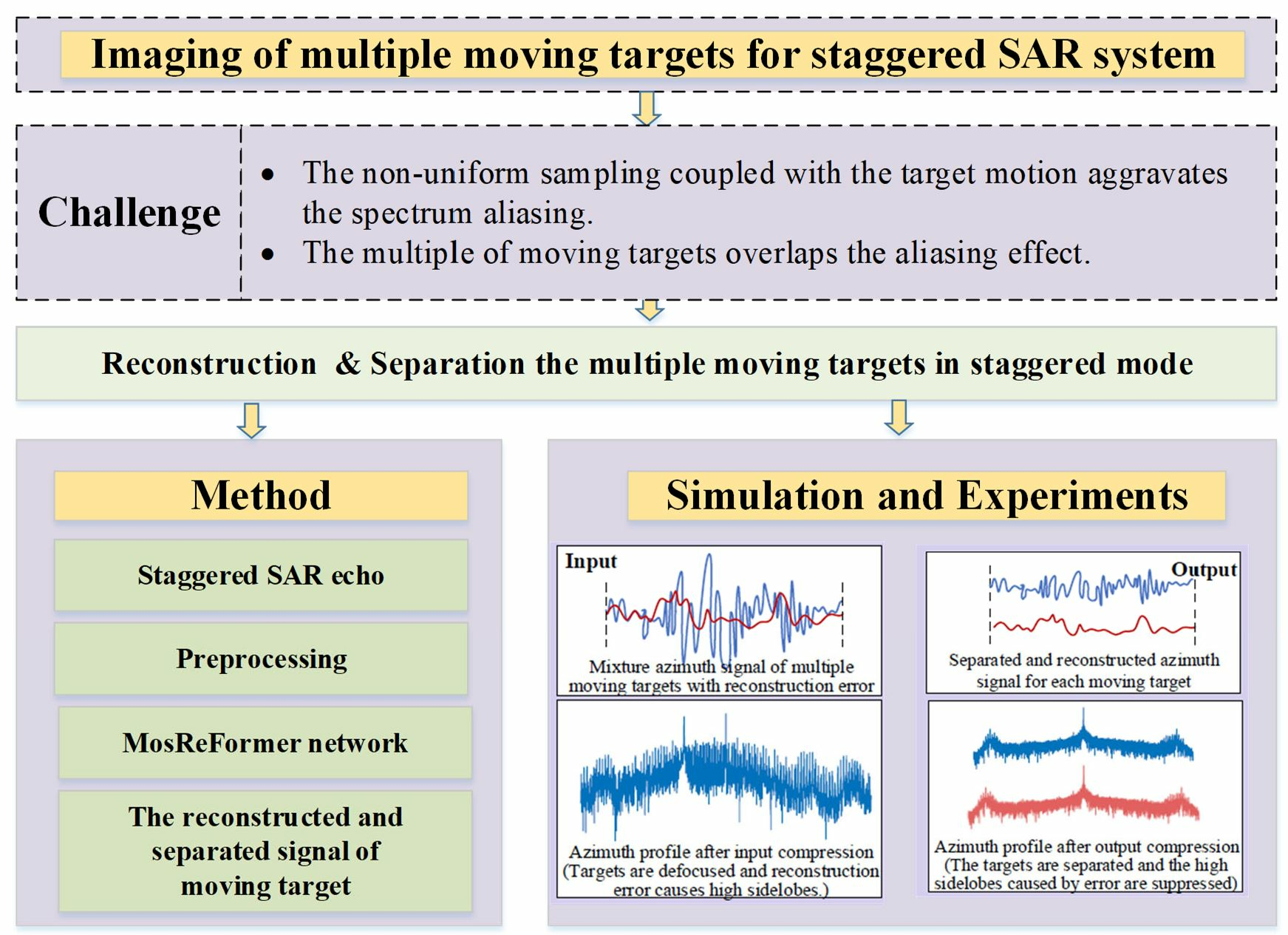
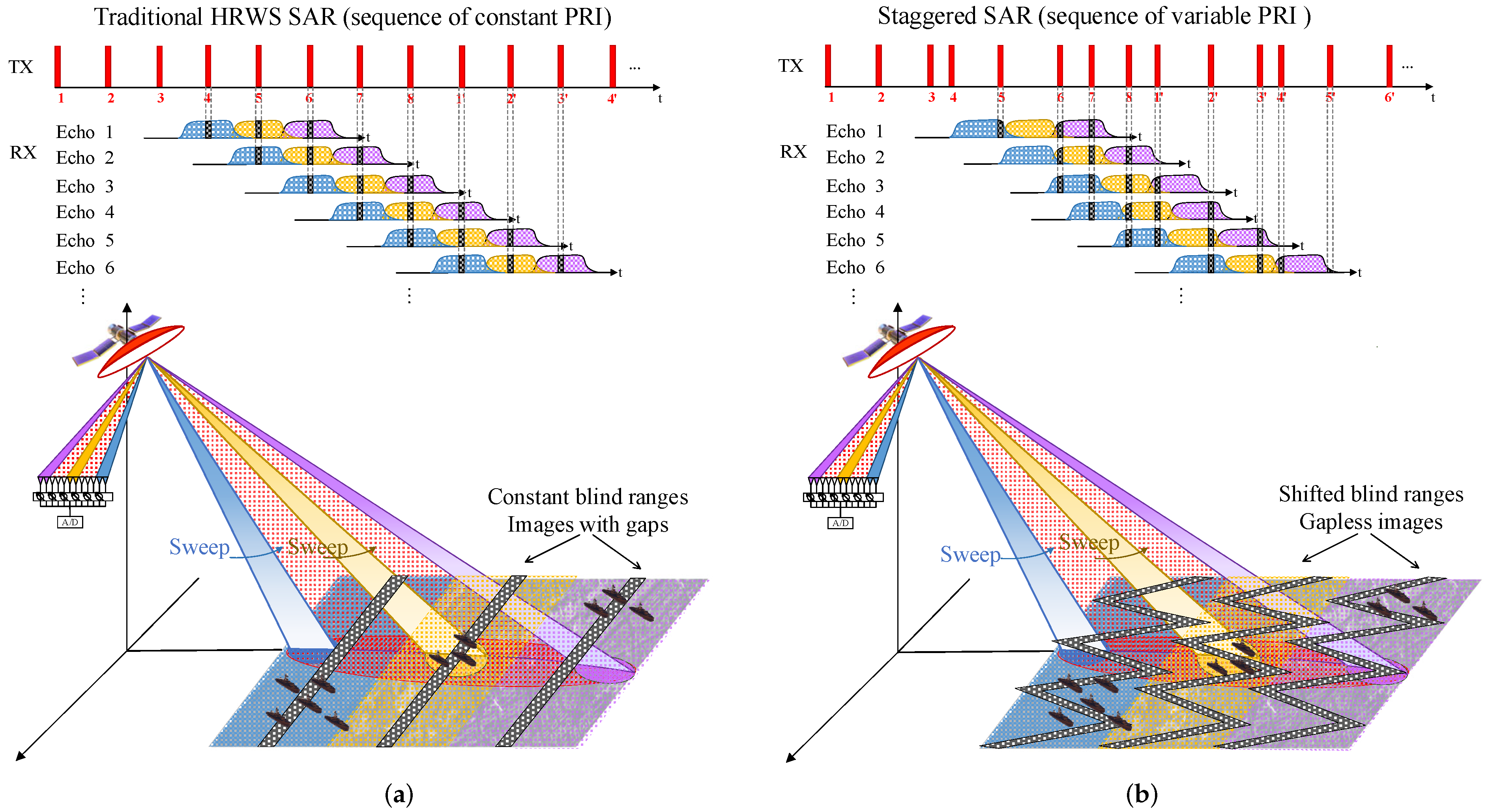
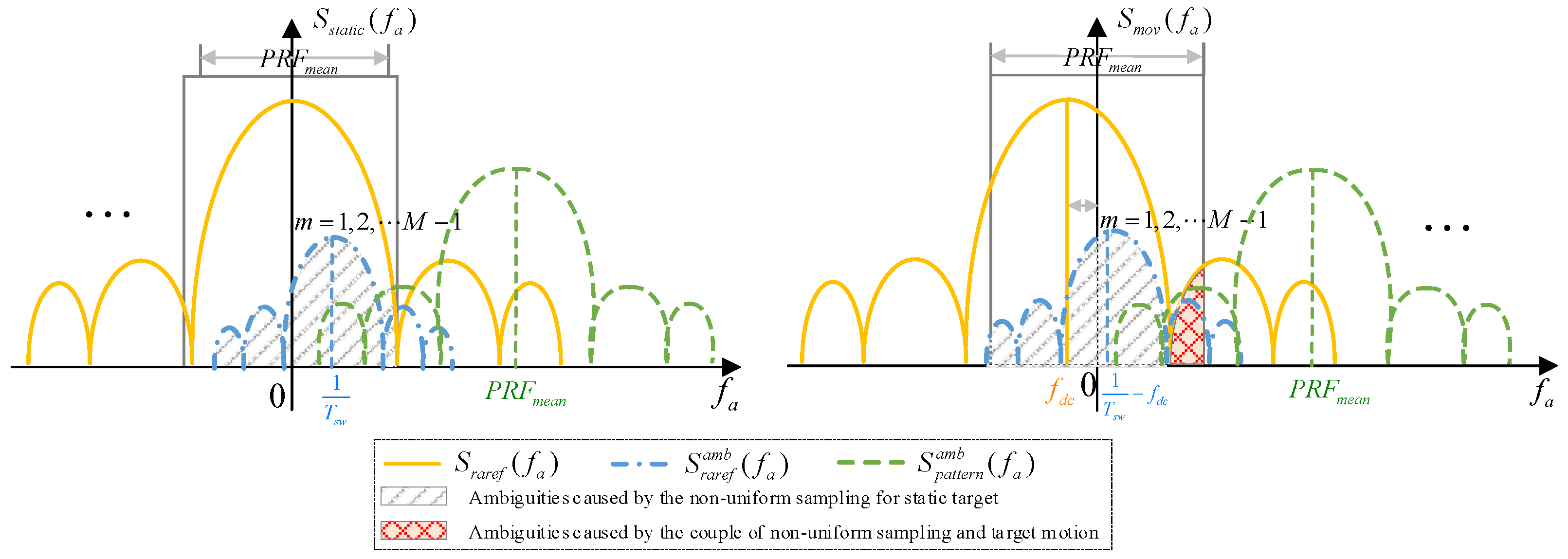
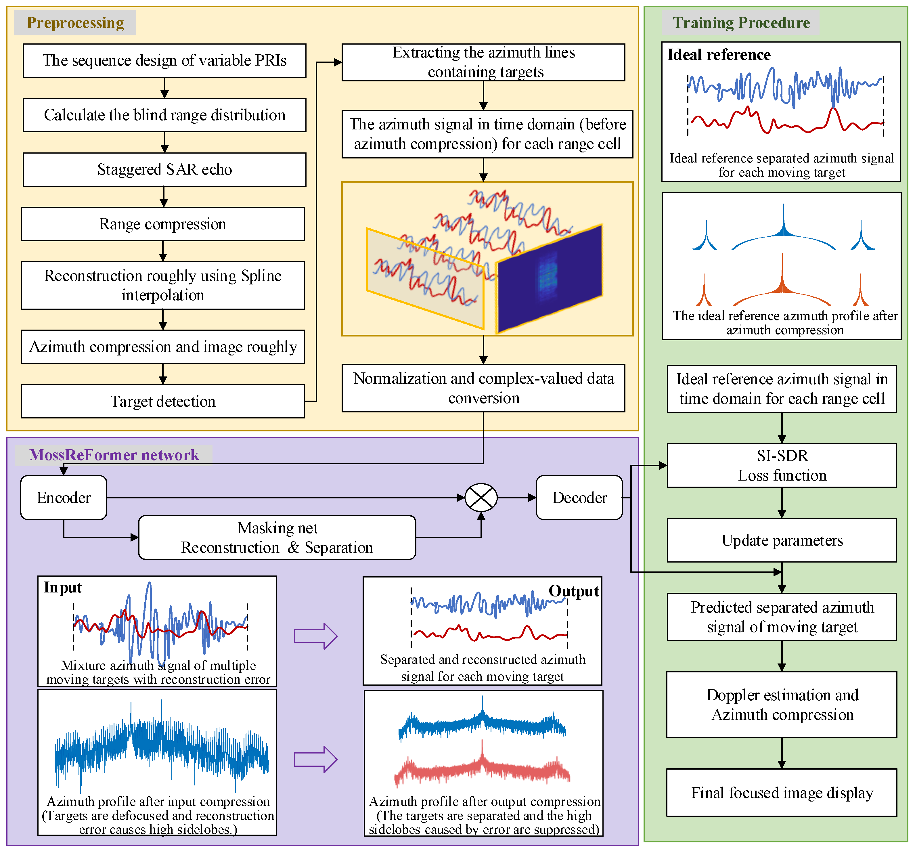
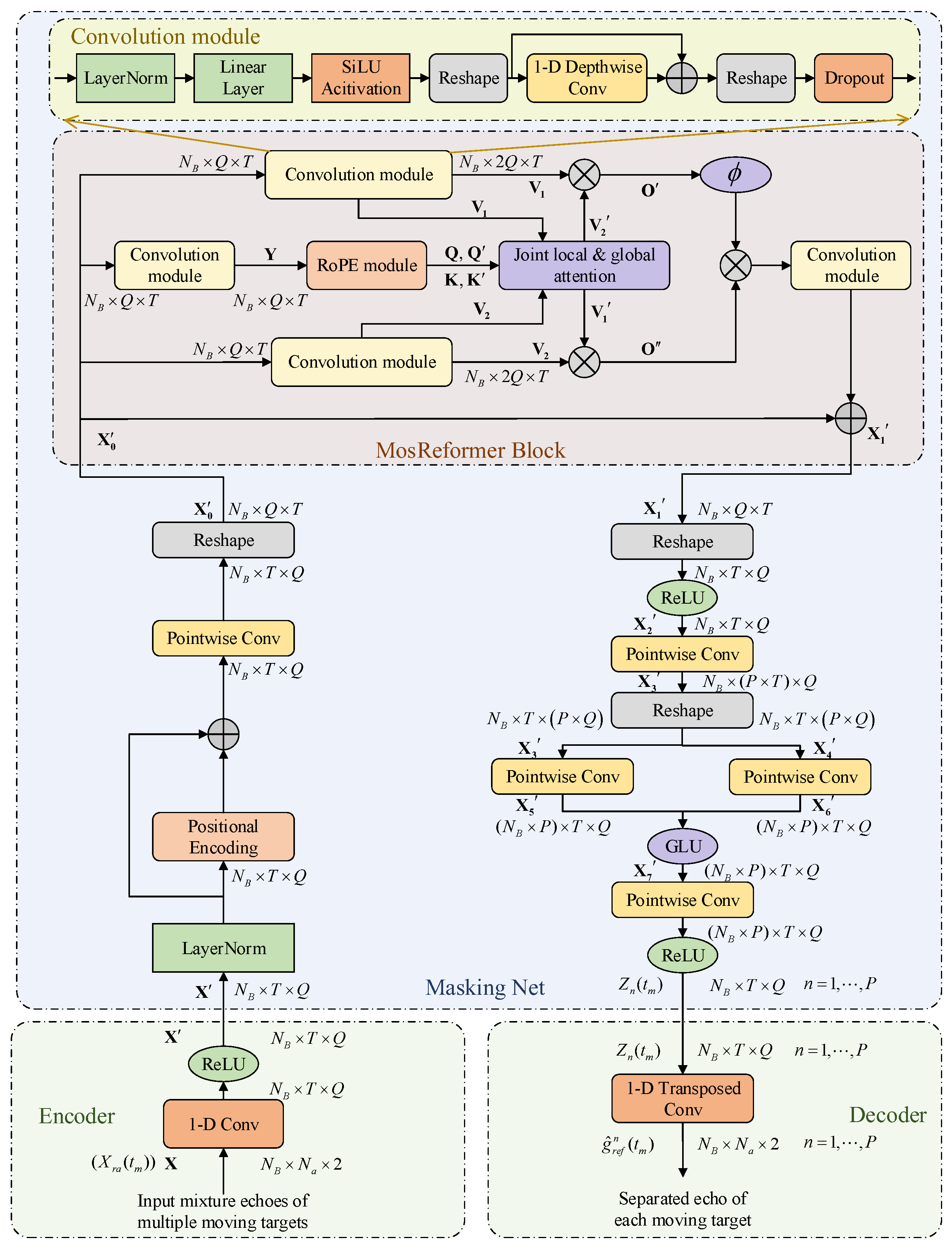
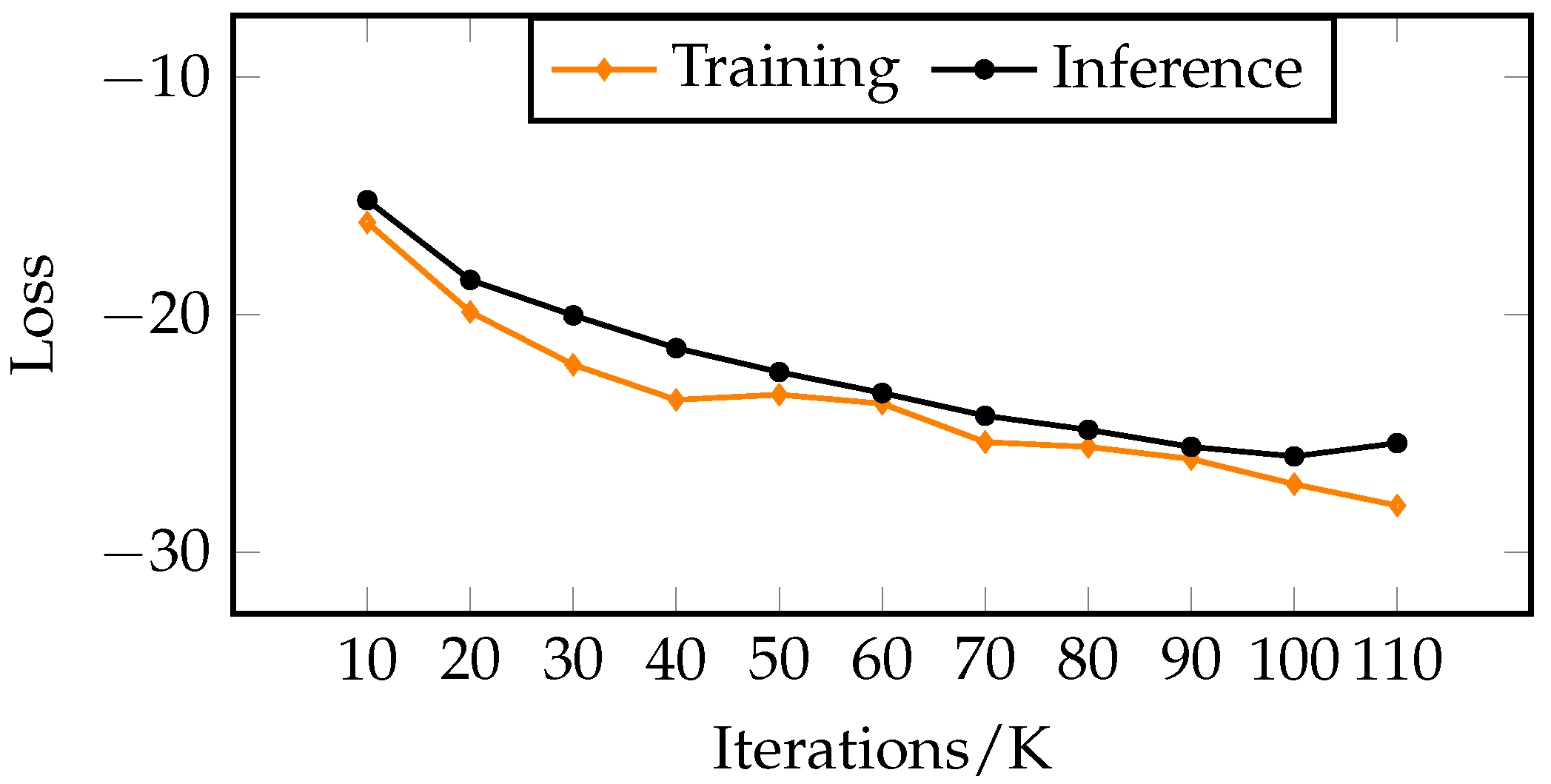
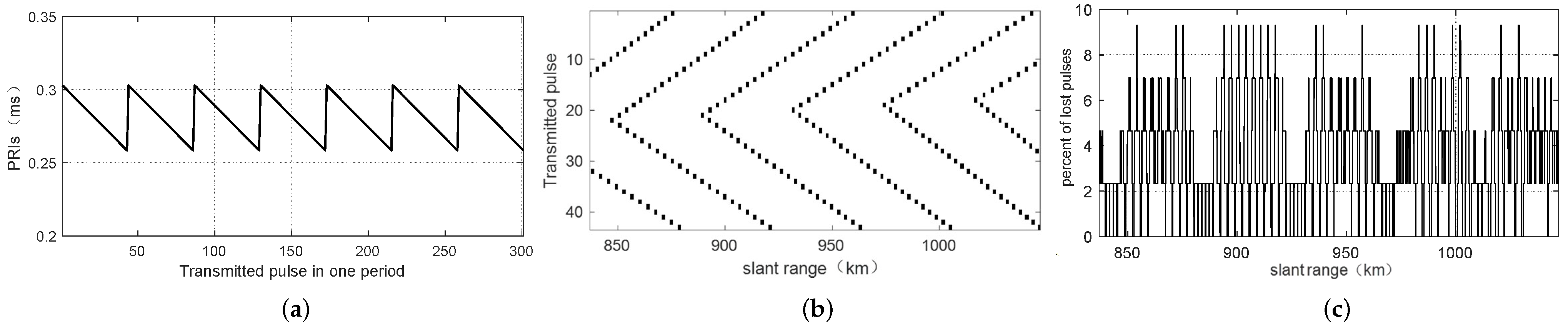
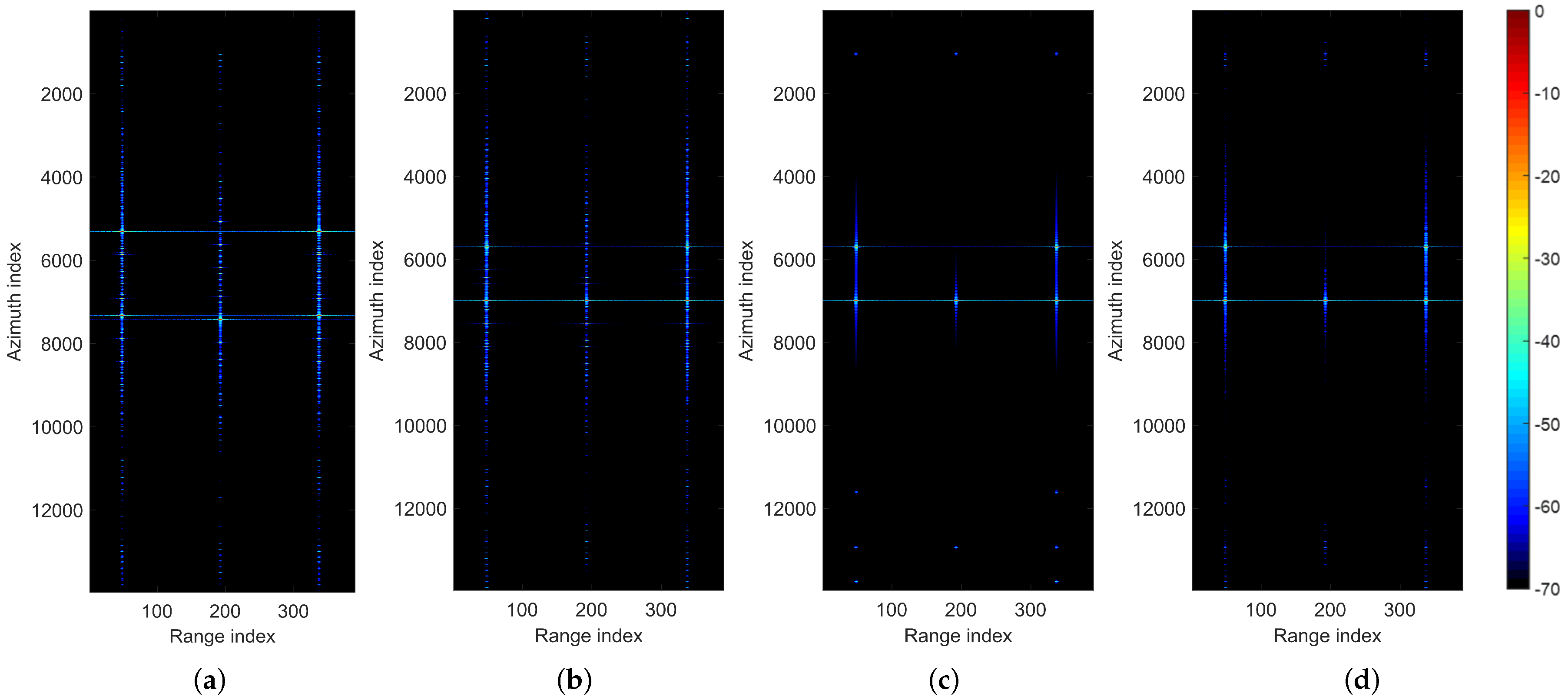
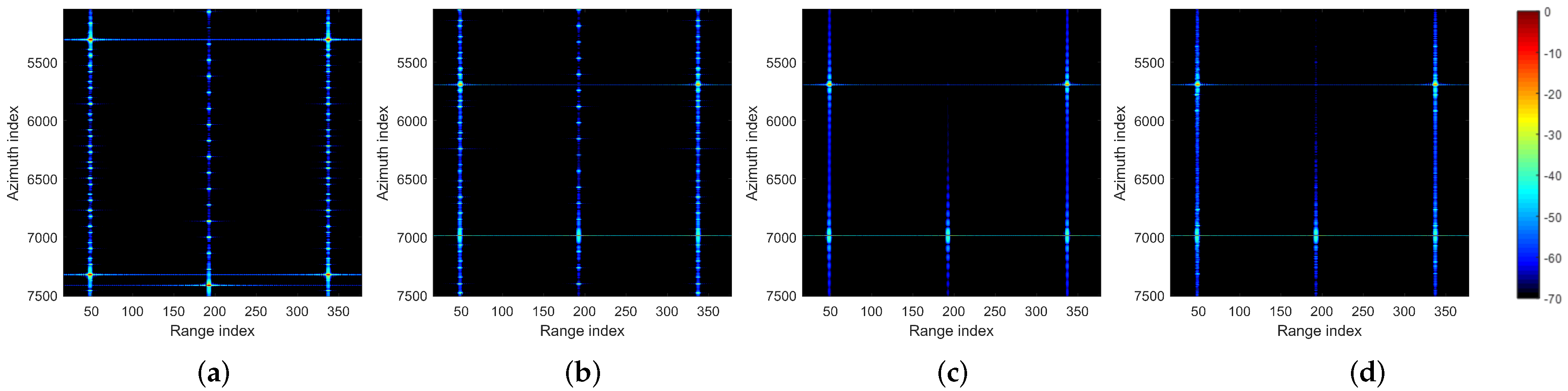
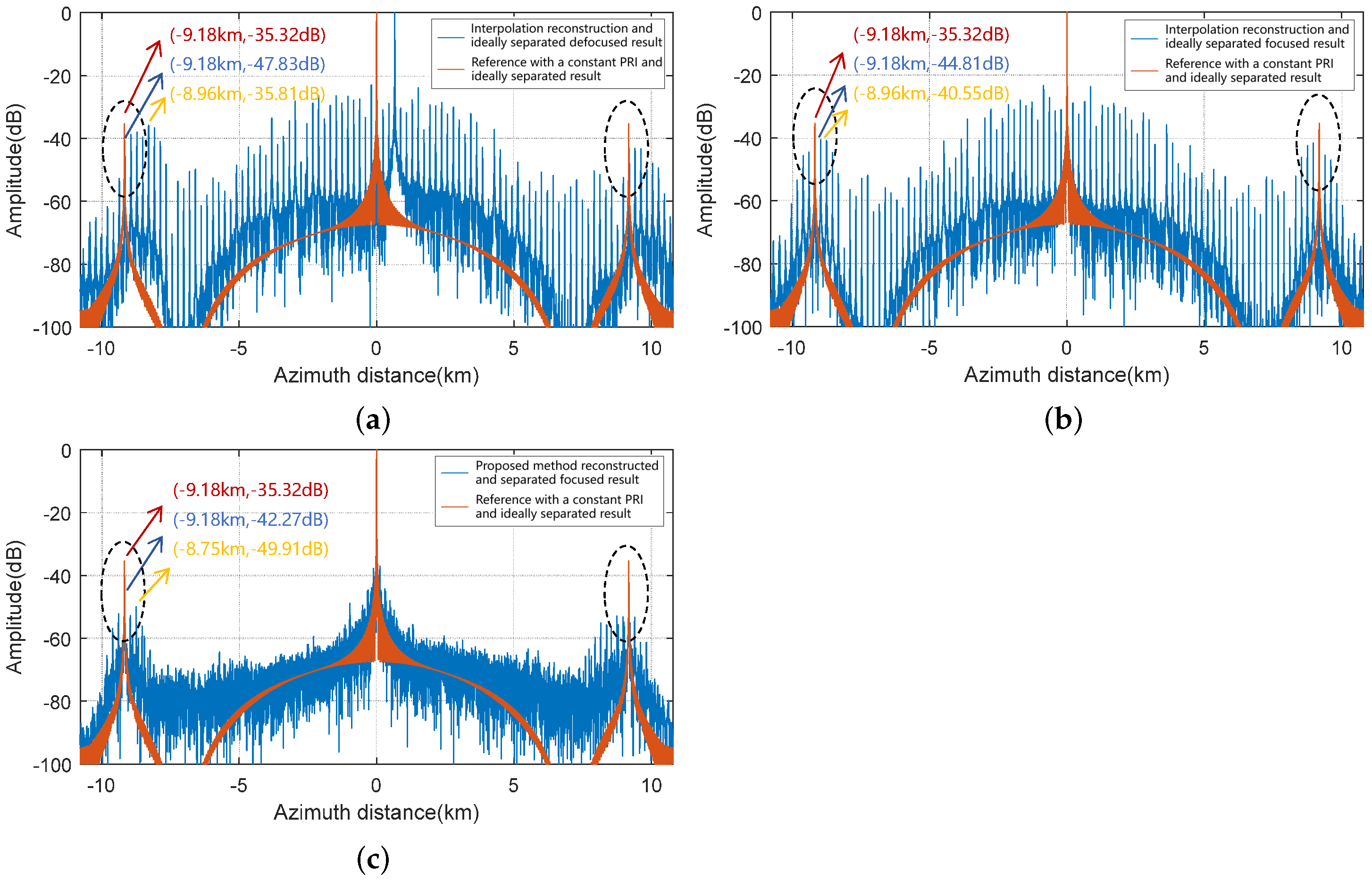
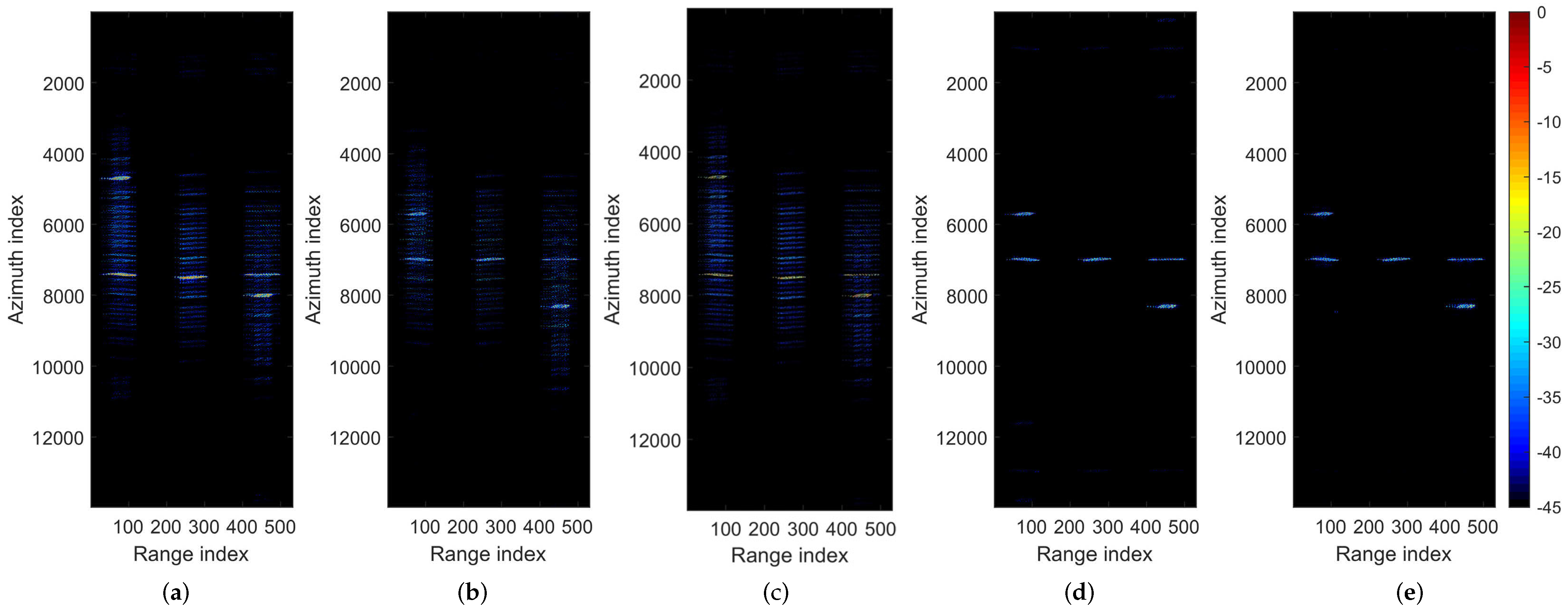
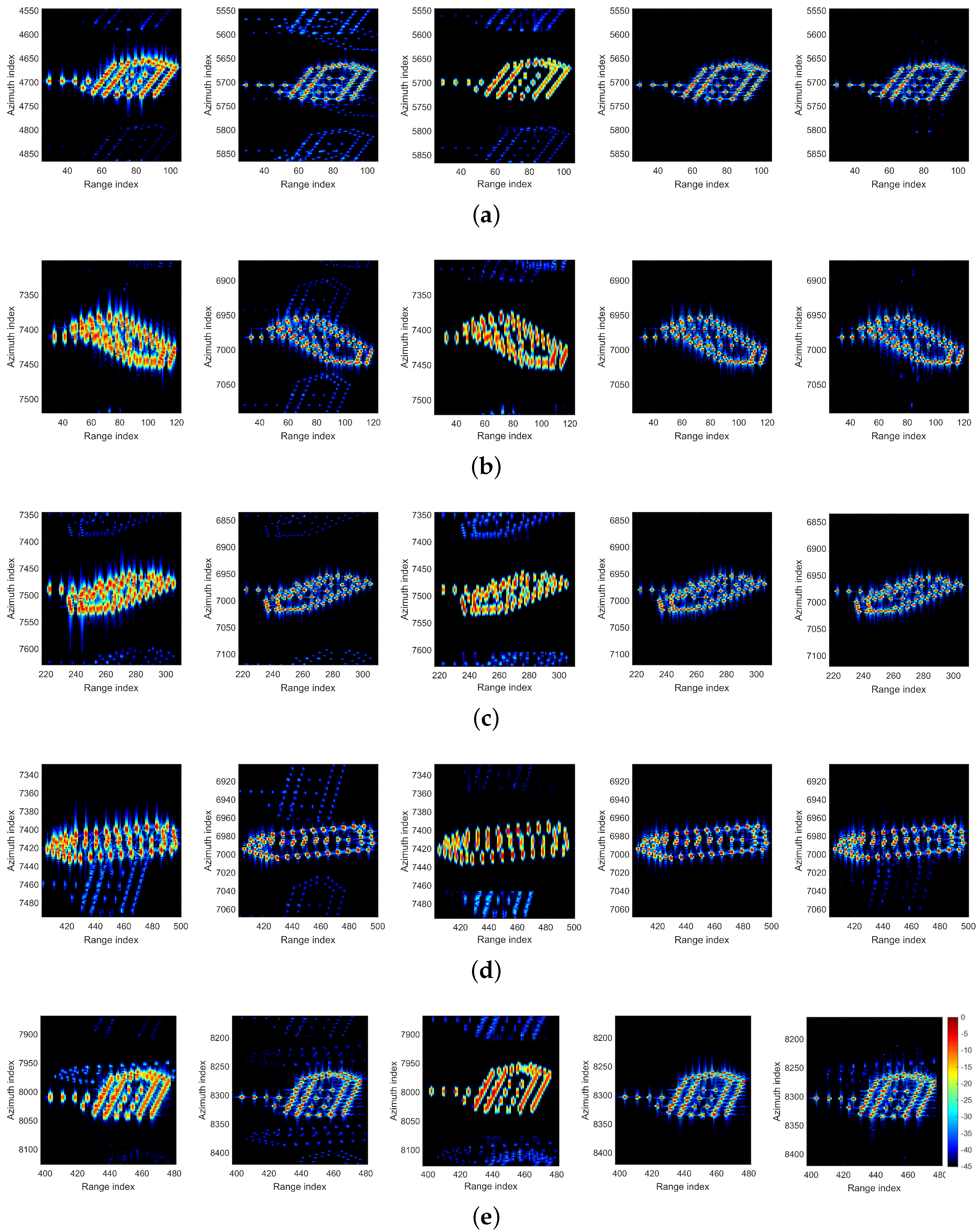
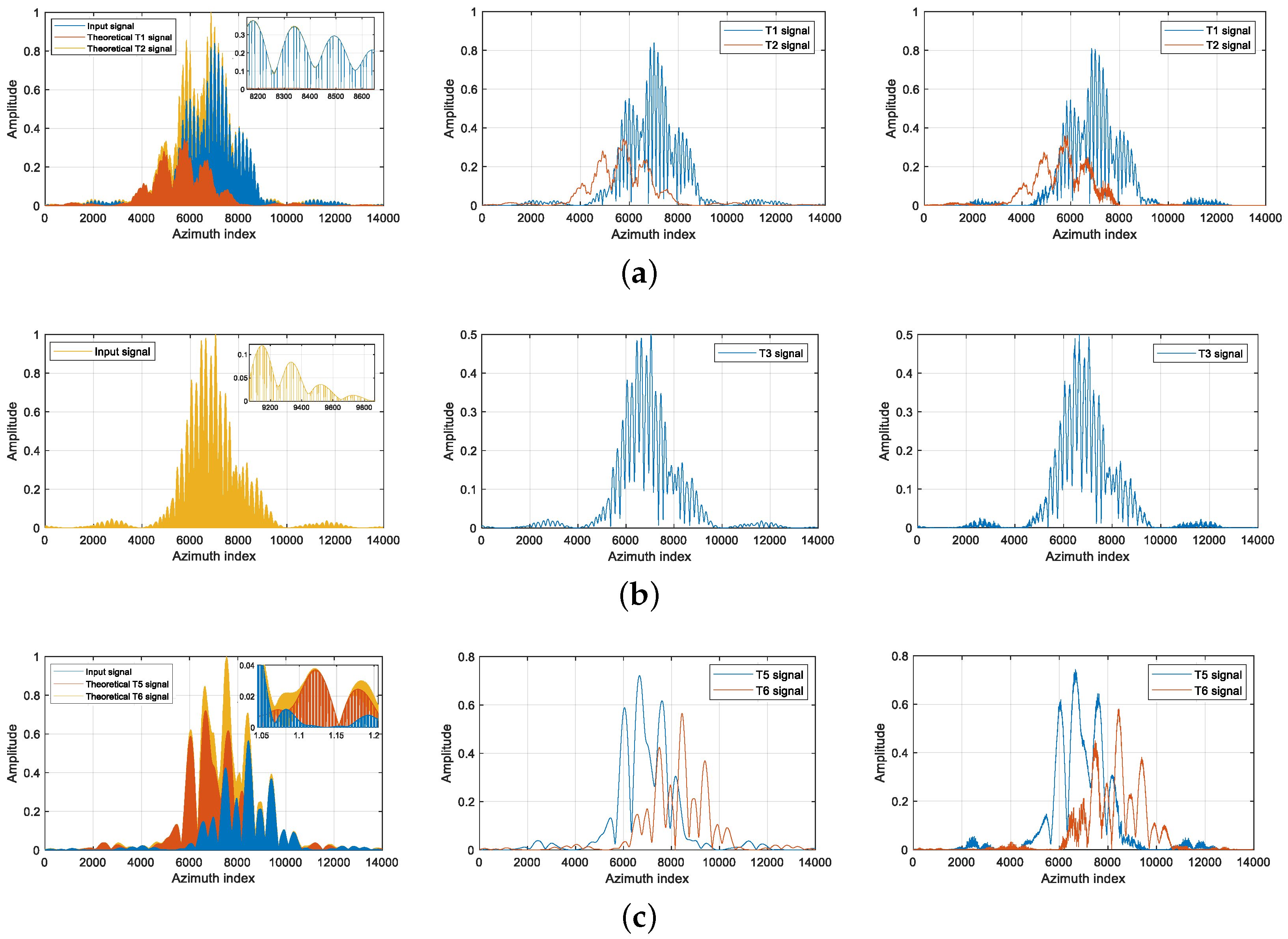
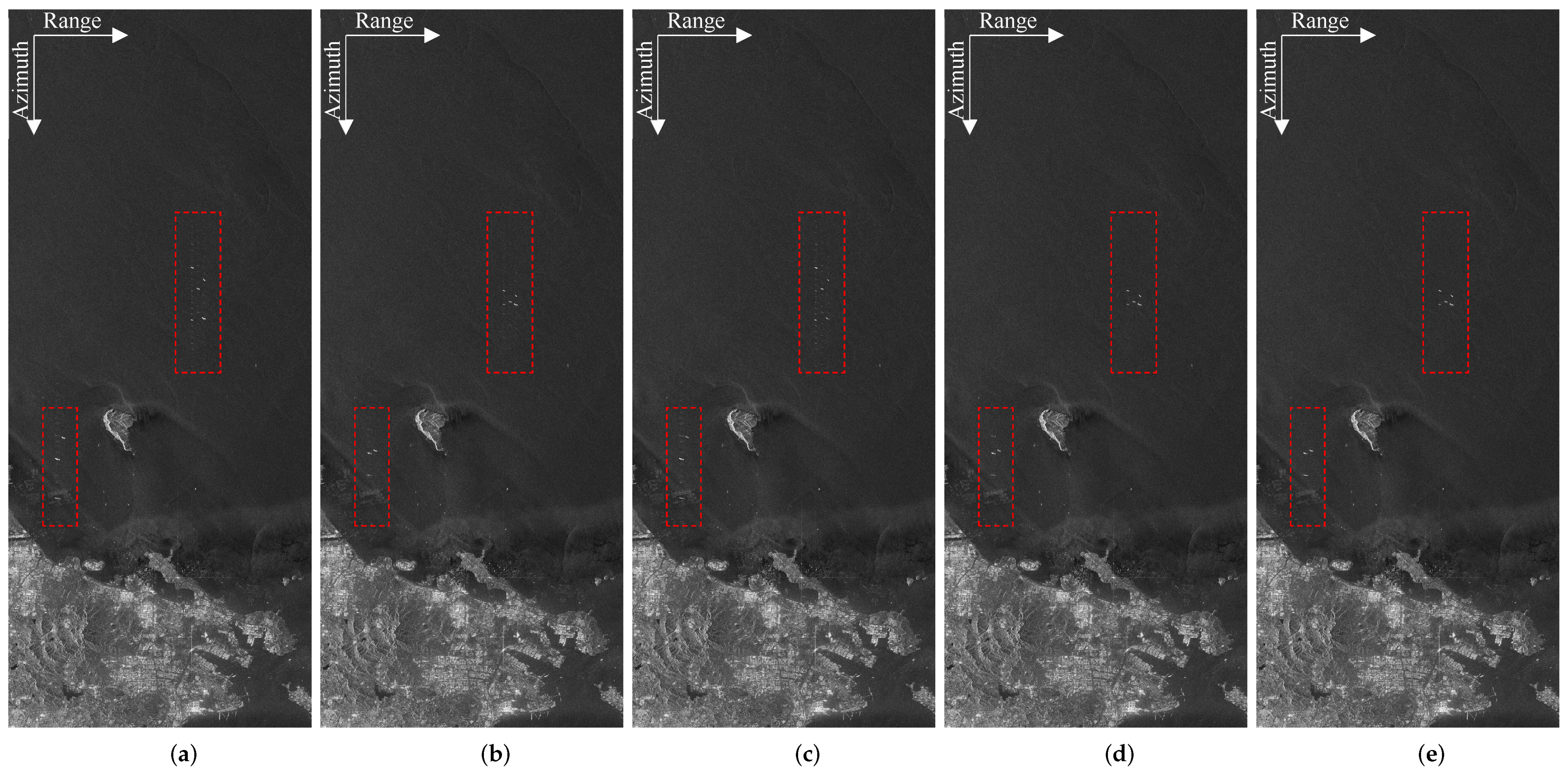
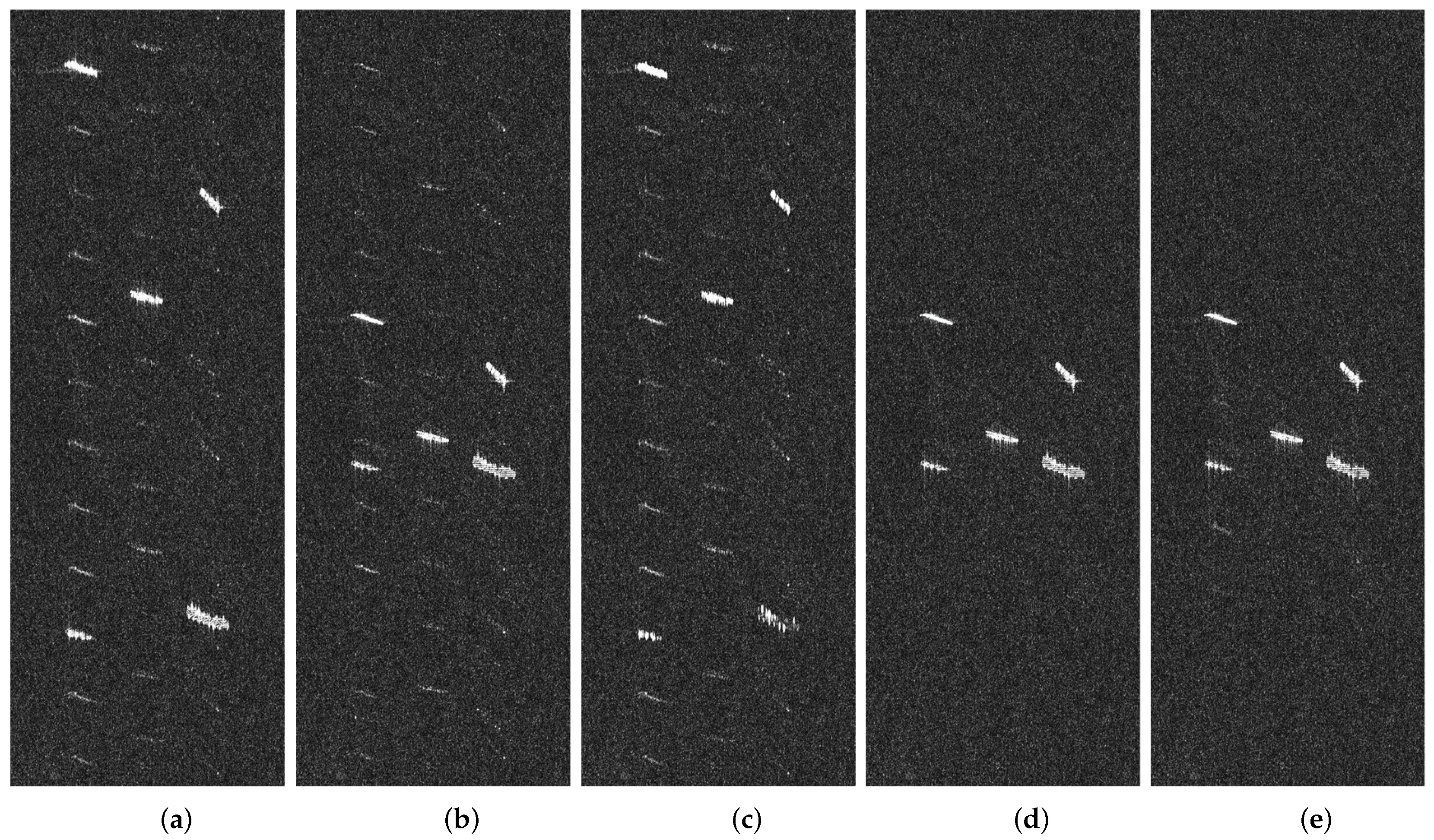
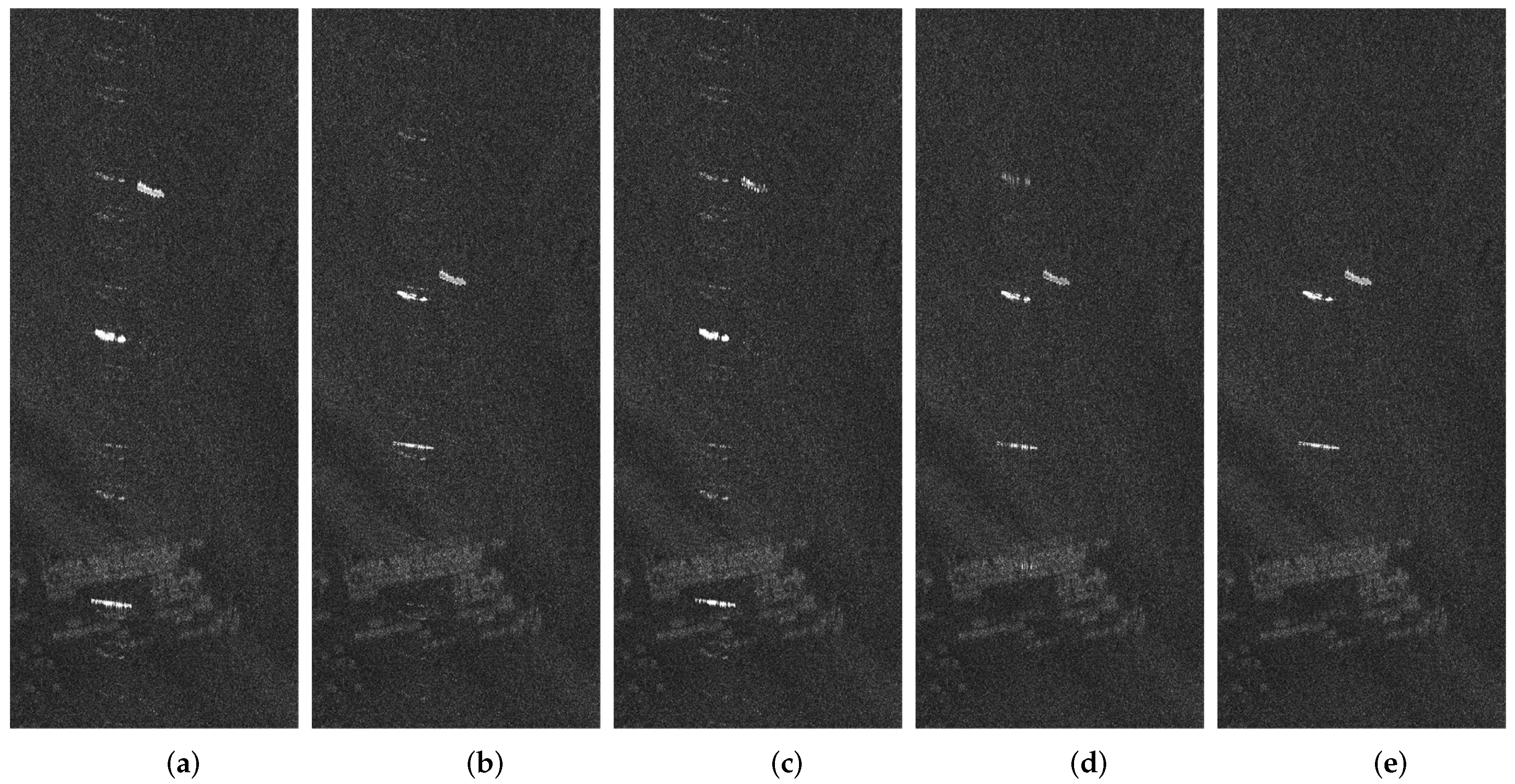
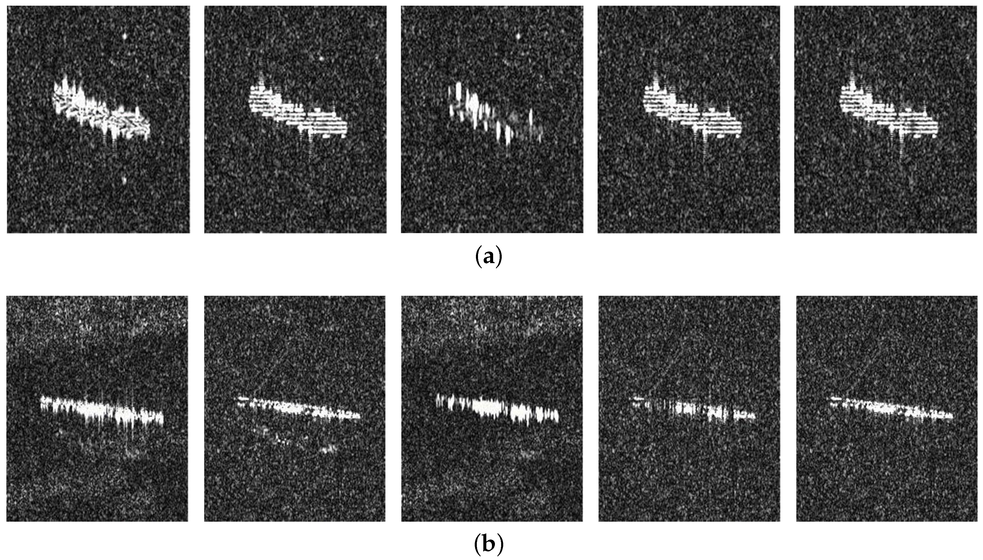
Table 1.
Simulation parameters in staggered SAR system.
| Parameter | Notation | Value |
|---|---|---|
| Carrier frequency | 9.6 GHz | |
| Orbit height | 760 km | |
| Off-nadir angle | 23.3°–40.5° | |
| Ground range coverage | 333–668 km | |
| Incidence angle | 26.3°–46.6° | |
| Range bandwidth | 180 MHz | |
| Transmitted pulse duration | 5 us | |
| Processed Doppler band | 2010 Hz | |
| Minimum PRF | 3300 Hz | |
| Maximum PRF | 3860 Hz | |
| The number of variable PRIs | M | 43 |
Table 2.
Configuration of the training process of the MosReFormer network.
| Setting Up | Value | Hyper-Parameters | Value |
|---|---|---|---|
| Batch Size | 10 | No.MosReFormer Blocks | 24 |
| Learning Rate | 0.001 | Encoder Output Dimension (Q) | 512 |
| Learning Rate Schedule | linear | Encoder Kernel Size ()/Stride | 16/8 |
| Warmup | 3000 | Depthwise Conv Kernel Size () | 17 |
| Normalization | Chunk Size (P) | 256 | |
| Gradient Clipping | 2 | Attention Dimension (d) | 128 |
| Dropout | 0.1 | Gating Activation Function | Sigmoid |
Table 3.
Imaging performance of moving point targets with different methods.
| Performance/Methods | DIRIS | IRIS | Ideal Reference | MosReFormer-Based Method |
|---|---|---|---|---|
| ISLR | −13.34 | −13.25 | −18.45 | −18.02 |
| PSLR | −23.09 | −23.40 | −35.38 | −37.08 |
| Entropy | 5.49 | 4.69 | 4.37 | 4.39 |
Table 4.
Imaging performance of simulated moving targets with different methods.
| Entropy | DIRIS | IRIS | RID | Ideal Reference | MosReFormer-Based Method |
|---|---|---|---|---|---|
| Target1 | 7.04 | 6.36 | 6.55 | 6.24 | 6.25 |
| Target2 | 7.43 | 6.35 | 7.01 | 6.31 | 6.32 |
| Target3 | 7.48 | 6.31 | 6.92 | 6.28 | 6.28 |
| Target4 | 6.72 | 6.05 | 6.33 | 6.01 | 6.02 |
| Target5 | 7.22 | 6.33 | 7.20 | 6.30 | 6.31 |
| All scene | 9.11 | 8.19 | 8.82 | 7.86 | 7.88 |
Table 5.
Imaging performance of the spaceborne SAR data with different methods.
| Performance | DIRIS | IRIS | RID | Ideal Reference | MosReFormer-Based Method |
|---|---|---|---|---|---|
| Entropy | 7.58 | 7.26 | 7.31 | 6.96 | 6.99 |
Disclaimer/Publisher’s Note: The statements, opinions and data contained in all publications are solely those of the individual author(s) and contributor(s) and not of MDPI and/or the editor(s). MDPI and/or the editor(s) disclaim responsibility for any injury to people or property resulting from any ideas, methods, instructions or products referred to in the content. |
© 2023 by the authors. Licensee MDPI, Basel, Switzerland. This article is an open access article distributed under the terms and conditions of the Creative Commons Attribution (CC BY) license (https://creativecommons.org/licenses/by/4.0/).
Share and Cite
MDPI and ACS Style
Qi, X.; Zhang, Y.; Jiang, Y.; Liu, Z.; Yang, C. MosReformer: Reconstruction and Separation of Multiple Moving Targets for Staggered SAR Imaging. Remote Sens. 2023, 15, 4911. https://doi.org/10.3390/rs15204911
AMA Style
Qi X, Zhang Y, Jiang Y, Liu Z, Yang C. MosReformer: Reconstruction and Separation of Multiple Moving Targets for Staggered SAR Imaging. Remote Sensing. 2023; 15(20):4911. https://doi.org/10.3390/rs15204911
Chicago/Turabian StyleQi, Xin, Yun Zhang, Yicheng Jiang, Zitao Liu, and Chang Yang. 2023. "MosReformer: Reconstruction and Separation of Multiple Moving Targets for Staggered SAR Imaging" Remote Sensing 15, no. 20: 4911. https://doi.org/10.3390/rs15204911
Note that from the first issue of 2016, this journal uses article numbers instead of page numbers. See further details here.