Novel Compact Polarized Martian Wind Imaging Interferometer

Abstract

The Mars Atmospheric Wind Imaging Interferometer offers several advantages, notably its high throughput, enabling the acquisition of precise and high vertical resolution data on the temperature and wind fields in the Martian atmosphere. Considering the current absence of such an Interferometer, this paper introduces a novel Mars wind field imaging interferometer. In analyzing the photochemical model of O₂ (a¹Δ_g) 1.27 μm molecular airglow radiation in the Martian atmosphere and considering the impact of instrument signal-to-noise ratio (SNR), we have chosen an optical path difference (OPD) of 8.6 cm for the interferometer. The all-solid-state polarized wind imaging interferometer is miniaturized by incorporating two arm glasses as the compensation medium in its construction, achieving the effects of field-widening and temperature compensation. Additionally, an F-P Etalon is designed to selectively filter the desired three spectral lines of O₂ dayglow, and its effect is evaluated through simulations. The accuracy of the proposed compact Mars polarized wind imaging interferometer for detecting Mars’ wind field and temperature field has been validated through rigorous theoretical derivation and comprehensive computer simulations. The interferometer boasts several advantages, including its compact and small size, static stability, minimal stray light, and absence of moving parts. It establishes the theoretical, technological, and instrumental engineering foundations for future simultaneous static measurement of Martian global atmospheric wind fields, temperature fields, and ozone concentrations from spacecraft, thereby significantly contributing to the dataset for investigating Martian atmospheric dynamics.

1. Introduction

Mars is the most similar planet to Earth in the solar system and is also considered the most likely planet to harbor life. The Mars atmospheric global remote sensing measurement is an important objective of Mars exploration. As the key parameter of Mars atmospheric dynamics, Mars’ wind field and temperature field play an important role in understanding the basic dynamic balance of the atmosphere, the basic transport process of Mars substances (such as dust, aerosols, and chemical components), the Mars ionospheric electrodynamics (Mars thermosphere-ionosphere coupling), and ensuring the safe landing of future unmanned spacecraft [1,2,3]. Currently, there is a lack of effective means for globally detecting the low-level atmospheric wind field on Mars, which seriously hinders the research of Mars atmospheric circulation and energy transport. It is urgent to achieve direct measurements of Mars’ atmospheric wind field.

Passive atmospheric wind field interferometric measurement technology has the advantages of long monitoring distance, wide range, and high wind field measurement accuracy. It has been successfully applied to the remote sensing of Earth’s atmospheric wind fields. This technology uses the airglow radiation generated by moving particles such as O₂, O, and OH in nature as the light source. The airglow spectrum produced by moving particles experiences Doppler shift as a result of atmospheric motion. This Doppler shift is detected and converted into Doppler phase measurements using an interferometer with a significant optical path difference (OPD), enabling the determination of line-of-sight wind velocity. The atmospheric temperature can be derived either by measuring the visibility of the interferogram or by utilizing rotational spectral lines.

Since the 1980s, scientists have developed various types of passive atmospheric wind field imaging interferometers. According to the principle and scheme, it can be classified into categories based on the F-P interferometer, wide-field Michelson interferometer, and non-symmetric spatial heterodyne interferometer (DASH). In 1991, NASA launched the Upper Atmosphere Research Satellite (UARS), which was jointly developed by Canada and France. The satellite carried the high-resolution Doppler imager (HRDI) [4] and the wind imaging interferometer (WINDII) [5,6], and conducted the first passive interferometric measurement of the Earth’s upper atmospheric wind field based on a satellite platform. WINDII is a dynamically scanned Michelson interferometer based on piezoelectric ceramics, which detects the wind field in the altitude range of 80–300 km in the Earth’s atmosphere. Subsequently, instruments with similar principles to WINDII were developed, including the ground-based thermospheric wind polarimetric Michelson interferometer (PAMI) [7], the ground-based E-region wind interferometer (ERWIN) [8], the stratospheric wind interferometer (SWIFT) [9], the atmospheric wave detection Michelson interferometer (WAMI) [10,11], the middle atmosphere imaging Michelson interferometer (MIMI) [12], the airglow dynamics Michelson interferometer (MIADI) [13], and the birefringent Doppler wind imaging interferometer (BIDWIN) [14] based on double-refracting crystals with four quadrants. As another wind measuring instrument carried on the UARS satellite, HRDI [4] is a Doppler imaging interferometer based on the F-P interferometer, which includes three combined F-P interferometers. It obtains atmospheric wind velocity through the doppler frequency shift and can detect atmospheric wind fields in the altitude range of 10–120 km above the Earth, with a vertical resolution of 6 km, a wind measurement accuracy of about 5 m/s, and a temperature measurement accuracy of about 7 K [15]. In 2001, the F-P interferometer-based wind imaging interferometer “Thermosphere-Ionosphere-Mesosphere Energetics and Dynamics Doppler Interferometer (TIDI)” [16,17] was successfully launched on the TIMED satellite. It is a new generation of high-resolution F-P interferometer-based spectral imaging instrument developed on the basis of the successful application of HRDI. Compared with the Michelson wind imaging interferometer, the F-P interferometer-based wind imaging interferometer technology has the disadvantages of small field of view, low transmittance, and extremely high requirements for the flatness of the standard, which makes it difficult to achieve high spatiotemporal resolution and high accuracy. The Doppler asymmetric spatial heterodyne (DASH) technique can also be used for passive measurement of Mars atmospheric wind fields. It was proposed by Englert et al. [18] from the US Navy Laboratory in 2006. By measuring the Doppler shift of spectral lines, the atmospheric wind field is retrieved, and high phase sensitivity is achieved by the large optical path difference of the asymmetric design of the interferometer arms. It uses the perfect Fourier transform relationship between the interferogram and the incident light spectrum to invert the Doppler frequency shift of the incident light spectrum by calculating the complex interferogram phase [19]. The representative instrument is the Michelson Interferometer for Global High-resolution Thermospheric Imaging (MIGHTI) [20,21], which was launched in 2019 and is used to detect the horizontal wind velocity profiles and thermospheric temperatures in the altitude range of 90–300 km. Due to the large OPD, the DASH technique has a large phase error in spectral recovery.

Currently, there are at least two proposed instrument schemes that are in the proposal stage for imaging Mars’ atmospheric wind fields, namely, the microwave and submillimeter-wave limb sounder [2,22,23] and the Doppler Michelson atmospheric dynamics interferometer (DYNAMO) [1,3]. Both of these instruments measure the Doppler shift of the absorption or the emission spectra of atmospheric molecules on Mars to obtain wind velocity information. The microwave and submillimeter-wave limb sounder is less affected by dust, ice clouds, and aerosols in the Martian atmosphere due to its longer wavelength. However, its wind velocity measurement accuracy is relatively low, with a typical accuracy of 15 m/s, and its vertical resolution is also limited, which restricts the fine description of vertical dynamic processes in the Martian atmosphere [1]. DYNAMO is a conceptual instrument proposed by W.E. Ward et al. [3] in 2002 for passive measuring Martian atmospheric information such as wind fields, temperature, and composition, among others. In 2021, Tao YU et al. [1] constructed a forward model for the DYNAMO instrument consisting of an orbit submodel, an atmospheric background field submodel, and an instrument submodel. A very detailed study was conducted on the principles of Martian atmospheric wind field monitoring, particularly the forward and inverse modeling, making it a valuable reference.

The key differentiation between passive remote sensing of Martian atmospheric wind fields and Earth’s atmospheric remote sensing resides in various factors: the distinct O₂ dayglow photochemical radiation model, variations in atmospheric composition and their altitudinal distributions, dynamic parameters such as temperature and wind speed, and the dissimilar atmospheric models present on Mars compared to Earth. Consequently, passive remote sensing of Martian atmospheric wind fields possesses unique attributes that call for a thorough reevaluation and redesign across aspects such as signal-to-noise ratio, instrument design, parameters, and more. Currently, there is a lack of static passive remote sensing wind imaging interferometers for simultaneous measurement of Martian global atmospheric wind fields, temperature fields, and ozone concentrations. This limitation significantly hinders our understanding of Martian atmospheric dynamics, energy and momentum transport, and wave behaviors, such as those of Martian gravity waves. In this paper, we inherited the previous work [11,14,24,25,26] of our research group on wind imaging interferometers and proposed a compact fully solid-state static polarized Martian wind imaging interferometer. The aim is to achieve miniaturization and efficient, static monitoring of wind fields. All components of the interferometer are securely bonded together to form a robust unit. By analyzing the signal-to-noise ratio (SNR), an optical path difference (OPD) of 8.6 cm is selected, which is shorter than DYNAMO [3] and MWIMI [24]. A two-arm-glass configuration is chosen as the compensating glass to achieve wide field of view, high throughput, temperature compensation, and miniaturization. An F-P Etalon is designed to selectively filter out the three spectral lines of O₂ (a¹Δ_g) at 1.27 μm dayglow so that rotational temperatures and band volume emission rates can be determined [3,10]. We validated the proposed approach through computer simulations and demonstrated the significance of denoising the interferograms. This miniaturized design offers excellent stability and combines static operation, compact size, reduced stray light, the absence of moving parts, and cost-effectiveness.

2. Principle

2.1. Photochemical Mechanism of O₂ 1.27 μm Dayglow and Nightglow on Mars

The airglow of O₂ (a¹Δ_g) molecule at 1.27 μm is the brightest airglow in the Martian atmosphere, which can be divided into dayglow and nightglow. The mechanisms for their generation are different. The O₂ (a¹Δ_g) dayglow at 1.27 µm was first detected on Mars by Noxon et al. [27] in 1976. It is a result of the solar ultraviolet (UV) photodissociation of ozone in the Martian atmosphere and can be used as a good tracer for atmospheric ozone abundance. The photodissociation process of ozone of O₂ (a¹Δ_g) molecules can be shown in Equation (1). The O₂ (a¹Δ_g) molecules can be quenched by collision with CO₂, which is widely present in the Martian atmosphere, as shown in Equation (2). The spontaneous emission of O₂ (a¹Δg) molecules is shown in Equation (3), which produces the 1.27 μm airglow radiation band. The O₂ (a¹Δ_g) 1.27 μm dayglow was observed by other ground-based observatories [24,28,29,30] and satellite-based instruments, e.g., the SPICAM instrument onboard the Mars Express satellite platform [31,32] and the Mars Express Observatoire pour la Minéralogie l’Eau, les Glaces et l’Activité (OMEGA) [33]. Fedorova et al. [32] found that maximal dayglow intensities are observed during late winter to early spring at high latitudes in both hemispheres, the local maxima being 30 mega-Rayleigh (MR) (1MR = 10¹² photons cm⁻² s⁻¹ column⁻¹).

$${\mathrm{O}}_3+\mathrm{h}\mathsf{\nu }(\mathsf{\lambda }<310 \mathrm{nm})\to {\mathrm{O}}_2({\mathrm{a}}^1{\mathsf{\Delta }}_{\mathrm{g}})+\mathrm{O}({}^1\mathrm{D})$$

(1)

$${\mathrm{O}}_2({\mathrm{a}}^1{\mathsf{\Delta }}_{\mathrm{g}})+\mathrm{C}{\mathrm{O}}_2\to {\mathrm{O}}_2({\mathrm{X}}^3{\mathsf{\Sigma }}_{\mathrm{g}})+\mathrm{C}{\mathrm{O}}_2$$

(2)

$${\mathrm{O}}_2({\mathrm{a}}^1{\mathsf{\Delta }}_{\mathrm{g}})\to {\mathrm{O}}_2({\mathrm{X}}^3{\mathsf{\Sigma }}_{\mathrm{g}}^{-})+\mathrm{h}\mathsf{\nu }(1.27 \mathsf{\mu }\mathrm{m})$$

(3)

As ozone photodissociation ceases after sunset, the excited O₂ (a¹Δ_g) molecules used to generate Martian nightglow [34] are products of the three-body recombination reaction of O atoms and CO₂ molecules, unlike the dayglow. As shown in Equation (4). The first detections of the O₂ (a¹Δ_g) nightglow in 2010 indicate that it is about two orders of magnitude less intense than the dayglow [34,35].

$$\mathrm{O}+\mathrm{O}+\mathrm{C}{\mathrm{O}}_2\to {\mathrm{O}}_2({\mathrm{a}}^1{\mathsf{\Delta }}_{\mathrm{g}})+\mathrm{C}{\mathrm{O}}_2$$

(4)

The emission rate $\epsilon =\frac{[O_2(a^1{\mathsf{\Delta }}_g)]}{\tau }$ is defined as the number of photons emitted per second per cm³ by excited O₂ (a¹Δ_g) molecules, where [ ] designate the number density for a given atmospheric species, and $\tau$ represents the radiative lifetime for O₂ (a¹Δ_g), which is a temperature-dependent variable and not precisely known. The typical Martian atmosphere temperatures within the altitude range of 10 to 60 km vary approximately from 130 to 250 K. In this paper, the designed Mars polarized wind imaging interferometer does not directly measure the radiance. The integrated radiance along the line of sight that enters its aperture is given by $I={\displaystyle \int \frac{\epsilon }{4\pi }}dz$, where I is measured in photons/cm²/s/sr. The resulting dayglow intensity in MR is determined as [31,36]

$$4\mathsf{\pi }I(\mathrm{MR})={10}^{-12}J{\displaystyle {\int }_0^{\infty }\frac{\left[O_3\right]dz}{1+\tau k_{c{o}_2}\left[C{O}_2\right]}},$$

(5)

where J is the integrated product of the ozone photolysis rate coefficient and quantum yield, which depends on the solar flux at the given location and time of observation. k_CO2 is the rate of collisional deactivation (or quenching coefficient) of O₂ (a¹Δ_g) by CO₂. The reaction rate k_CO2 = 10⁻²⁰ cm⁻³ molecule⁻¹s⁻¹ and the radiative lifetime have been a subject of multiple studies [28,32,33,34,35,36,37,38,39,40]. Krasnopolsky [28] used value k_CO2 = 10⁻²⁰ cm⁻³ molecule⁻¹s⁻¹.

For nightglow, the emittance rate [34] can be derived from the mechanism of nightglow generation expressed by Equations (3) and (4).

$$\epsilon =\frac{k_1\beta [O][O]\left[C{O}_2\right]}{1+\mathsf{\tau }{k}_{c{o}_2}\left[C{O}_2\right]},$$

(6)

where k₁ is the rate coefficient of the three-body recombination reaction, and β is the yield rate of O₂ (a¹Δ_g) in the three-body recombination reaction. In the atmospheric science community, rate coefficient k₁ has been adopted widely, as in [28,34]. Crisp et al. [41] estimated that a yield rate β is about 0.6~0.75. The intensity of O₂ (a¹Δ_g) dayglow is about two orders of magnitude higher than nightglow, and it is closely related to the abundance of ozone, which can be retrieved from its photochemical model. Therefore, the compact polarized Martian wind imaging interferometer proposed in this paper mainly measures the Martian O₂ (a¹Δ_g) dayglow.

Due to the presence of hundreds of vibration–rotation spectral lines in the O₂ (a¹Δ_g) 1.27 μm dayglow radiation band, one needs to selectively choose a few spectral lines for the measurement of Martian atmospheric wind field using optical filtering. The selection of spectral lines follows the methodology of DYNAMO [3] and MWIMI [24], with 1264.060 nm, 1264.277 nm, and 1264.386 nm selected as the probe spectral lines. The details of these radiation lines are shown in

Table 1. Emission lines for the O₂ (a¹Δ_g) dayglow observations [3,10,24].

Line	Wavelength in Vacuum (nm)	Relative Intensity at 225 K	dI/dT at 225 K (%/K)
RQ (9)	1264.060	0.019	−0.016
SR (3)	1264.277	0.017	−0.340
RR (9)	1264.386	0.023	−0.016

. These three spectral lines are easy to filter using optical methods, have relatively high line strengths compared to other lines, and their line strengths exhibit different temperature sensitivities (dI/dT), making them suitable for rotational line temperature measurements. In addition, the Doppler frequency shift caused by the wind velocity is the same for each line, which allows them to be used for measuring line-of-sight wind velocity.

2.2. Principle of Polarized Martian Wind Imaging Interferometer

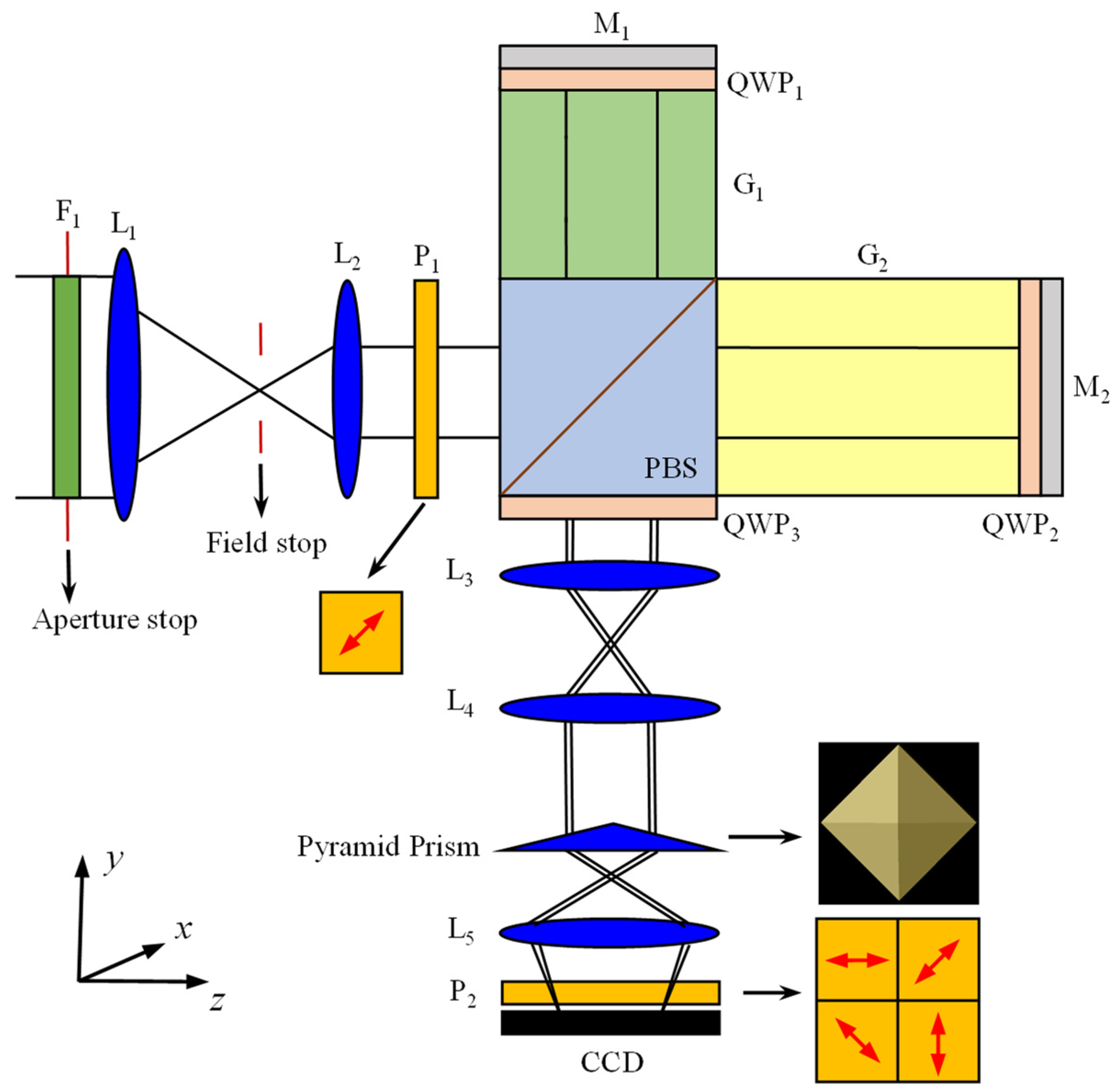
The schematic diagram of the polarized Martian wind imaging interferometer is shown in Figure 1. It consists of a filter, a front-end telescope system, a polarized wide-field Michelson interferometer, and a static four-zone imaging system. Filter F₁, consisting of a narrowband interference filter and an F-P Elton, is placed at the aperture stop to filter out the three selected spectral lines of O₂ (a¹Δ_g) 1.27 μm dayglow. The front-end telescope system has a magnification greater than 1 to collect more light. The field stop is placed at the focus of telescope L₁ to limit the field of view and filter out stray light. L₂ is a collimating lens, and it, together with lens L₁, forms the front-end telescope system. It collimates the incoming beam, matching its diameter with that of the interferometer module. The polarized wide-field Michelson interferometer is the core component, consisting of a linear polarizer P₁, three quarter-wave plates (QWP), a polarizing beam splitter (PBS), a linear polarizer array P₂, two arm glasses, G₁ and G₂, and two total reflection mirrors, M₁ and M₂. Its main function is to produce four interferograms with different phase steps. The transmission axis direction of P₁ is at a 45° angle with the positive x-axis, and the fast axis direction of the three QWPs is also at a 45° angle with the positive x-axis. The linear polarizer array consists of four linear polarizers with different transmission axes at 0°, 45°, 90°, and 135° with respect to the x-axis, which is used to achieve a four-step phase shift. The specific principles will be explained using the Jones calculus method below. The imaging system mainly consists of a rear-end telescope system (including lenses L₃ and L₄), a pyramid prism, an imaging mirror L₅, and a CCD detector.

After passing through the filter, the incident light enters the instrument and encounters a 45° linear polarizer after passing through the front-end telescope system, which splits the light into horizontal (p-component) and vertical polarized light (s-component) with equal amplitude. After passing through the polarizing beam splitter (PBS), the s-polarized light is reflected, while the p-polarized light is transmitted. The s-polarized light in the first path passes through QWP₁ and is reflected by the mirror before passing through QWP₁ again, which is equivalent to passing through a half-wave plate and rotating the polarization direction from s to p, thus transmitting through the PBS. Similarly, the p-polarized light in the second path passes through QWP₂ twice, changing its polarization direction to s, and then is reflected by the reflecting film of the PBS and exits the PBS. The two beams of light produce a phase difference after passing through QWP₃ and generate polarized interferometry with different phase steps through the linear polarizer array, and finally, the interferogram is imaged on the CCD.

We use the Jones matrix method and the principle of coherent superposition of light to calculate the wind field interferogram. The transmission axis direction between the linear polarizer P₁ and the positive x-axis is 45°. The Jones vector of the light transmitted through P₁ can be represented as ${\mathbf{E}}_0=\frac{1}{\sqrt{2}}\left(\begin{array}{l}1\\ 1\end{array}\right)$. After passing through the PBS, light is divided into reflected and transmitted light with polarization directions perpendicular to each other. Therefore, the PBS can be equivalent to two linear polarizers with polarization directions of 90° and 0° relative to the positive x-axis, respectively. Their Jones matrices are denoted as J_PBSr and J_PBSt, respectively. The function of QWP₁ and QWP₂ is equivalent to a half-wave plate with a fast axis direction of 45°, and their Jones matrices are represented by J_HWP. The fast axis direction of QWP₃ is also 45°, and its Jones matrix is represented by JQWP. The light vector from the QWP₃ can be represented by the reflected light vector E_r and the transmitted light vector E_t, which, respectively, can be expressed based on the Jones calculation as

$${\mathbf{E}}_{\mathrm{r}}={\mathrm{J}}_{\mathrm{QWP}}{\mathrm{J}}_{\mathrm{HWP}}{\mathrm{J}}_{{\mathrm{PBS}}_{\mathrm{r}}}{\mathbf{E}}_0=\frac{1}{2}\left(\begin{array}{l}1\\ -i\end{array}\right)$$

(7)

$${\mathbf{E}}_{\mathrm{t}}={\mathrm{J}}_{\mathrm{QWP}}{\mathrm{J}}_{\mathrm{HWP}}{\mathrm{J}}_{{\mathrm{PBS}}_{\mathrm{t}}}{\mathbf{E}}_0=\frac{1}{2}{\mathrm{e}}^{-i\frac{\pi }{2}}\left(\begin{array}{l}1\\ i\end{array}\right).$$

(8)

The reflected and transmitted light can be decomposed into their x and y components, resulting in the expressions for E_rx, E_ry, E_tx, and E_ty in Equations (9)–(12):

$${\mathbf{E}}_{\mathrm{rx}}=\frac{1}{2}A\exp [i(\mathbf{k}\cdot {\mathbf{r}}_1-\omega t)]$$

(9)

$${\mathbf{E}}_{\mathrm{ry}}=\frac{1}{2}A\exp [i(\mathbf{k}\cdot {\mathbf{r}}_1-\omega t)]\exp (-i\frac{\pi }{2})$$

(10)

$${\mathbf{E}}_{\mathrm{tx}}=\frac{1}{2}A\exp [i(\mathbf{k}\cdot {\mathbf{r}}_2-\omega t)]$$

(11)

$${\mathbf{E}}_{\mathrm{ty}}=\frac{1}{2}A\exp [i(\omega t-\mathbf{k}\cdot {\mathbf{r}}_2)]\exp (i\frac{\pi }{2}),$$

(12)

where A is the amplitude, w is the angular frequency, k is the wave vector of the incident light, and r₁ and r₂ represent the position vectors of reflected and transmitted light. Summing up the x and y components of the reflected and transmitted light, the electric field vector along the x and y directions can be obtained as shown in Equations (13) and (14):

$${\mathbf{E}}_x={\mathbf{E}}_{\mathrm{rx}}+{\mathbf{E}}_{\mathrm{tx}}=A\cos [\frac{\mathbf{k}\cdot ({\mathbf{r}}_1-{\mathbf{r}}_2)}{2}]\exp [i(\frac{\mathbf{k}\cdot ({\mathbf{r}}_1+{\mathbf{r}}_2)}{2}-\omega t)]$$

(13)

$${\mathbf{E}}_y={\mathbf{E}}_{\mathrm{ry}}+{\mathbf{E}}_{\mathrm{ty}}=A\sin [\frac{\mathbf{k}\cdot ({\mathbf{r}}_1-{\mathbf{r}}_2)}{2}]\exp [i(\frac{\mathbf{k}\cdot ({\mathbf{r}}_1+{\mathbf{r}}_2)}{2}-\omega t)].$$

(14)

According to the principle of polarization interference, the electric field vector on the detector can be expressed as

$${\mathbf{E}}_{out}={\mathbf{E}}_x\cos {\theta }_i+{\mathbf{E}}_y\sin {\theta }_i=A\exp [i(\frac{\mathbf{k}\cdot ({\mathbf{r}}_1+{\mathbf{r}}_2)}{2}-\omega t)]\cos (\frac{\mathbf{k}\cdot ({\mathbf{r}}_1-{\mathbf{r}}_2)}{2}-{\theta }_i),$$

(15)

where the angle θ_i (i = 1, 2, 3, 4) represents the angle between the linear polarizer in a polarizing array P₂ and the x-axis. As shown in Figure 1, θ_i = 0°, 45°, 90°, 135°.

Finally, the intensities measured by CCD can be expressed as

$$I_{out}={\mathbf{E}}_{out}\cdot {{\mathbf{E}}_{out}}^{*}=A^2{\cos }^2(\frac{\mathbf{k}\cdot ({\mathbf{r}}_1-{\mathbf{r}}_2)}{2}-{\theta }_i)=\frac{A^2}{2}[1+\cos (\mathbf{k}\cdot ({\mathbf{r}}_1-{\mathbf{r}}_2)-2{\theta }_i)],$$

(16)

where $\mathbf{k}\cdot ({\mathbf{r}}_1-{\mathbf{r}}_2)=2\pi \sigma {\mathsf{\Delta }}_0.$ ${\mathsf{\Delta }}_0$ is the optical path difference (OPD) between the two arms of the interferometer. $\sigma$ is the wavenumber. Assuming that I₀ represents the total incident light intensity, and the intensity is reduced by half after passing through P₁, Equation (16) can be expressed as

$$I_{out}=\frac{I_0}{4}[1+\cos (2\pi \sigma {\mathsf{\Delta }}_0-2{\theta }_i)].$$

(17)

To account for the doppler frequency shift caused by the line-of-sight wind, the phase term ${\varphi }_w$ needs to be added to Equation (17), which can be related to the wind velocity v as follows:

$${\varphi }_w=2\pi {\sigma }_0\mathsf{\Delta }v/c,$$

(18)

where v is the line-of-sight velocity of the source and c is the velocity of light. σ₀ corresponds to the wave number for zero wind velocity.

Considering that the actual detected spectral line is a Gaussian line shape, the fringe visibility V related to the spectral line broadening needs to be introduced in Equation (17). Due to the imperfections of the instrument modulation, such as tilt, the instrument visibility U also needs to be added. Therefore, Equation (17) can be rewritten as

$$I_{out}=\frac{I_0}{4}[1+UV\cos (2\pi \sigma {\mathsf{\Delta }}_0+{\varphi }_w-2{\theta }_i)].$$

(19)

By modulating with the linear polarizing array P₂, the detector can obtain four interferograms with different phase steps, which are represented by Equations (20)–(23).

$$I_1=\frac{I_0}{4}(1+UV\cos \psi )$$

(20)

$$I_2=\frac{I_0}{4}(1+UV\sin \psi )$$

(21)

$$I_3=\frac{I_0}{4}(1-UV\cos \psi )$$

(22)

$$I_4=\frac{I_0}{4}(1-UV\sin \psi ),$$

(23)

where $\psi =2\pi \sigma {\mathsf{\Delta }}_0+{\varphi }_w.$ According to the “Four-intensity method”, the basic parameters of the interferogram can be solved as shown below.

$$I_0=2\left(I_1+I_3\right)=2\left(I_2+I_4\right)$$

(24)

$$V=2{\left[{\left(I_1-I_3\right)}^2+{\left(I_4-I_2\right)}^2\right]}^{1/2}/U{I}_0$$

(25)

$$\tan \psi =\left(I_4-I_2\right)/\left(I_1-I_3\right)$$

(26)

After obtaining the wind phase term ${\varphi }_w$, the actual wind velocity can be determined according to Equation (18). The fringe visibility is closely related to atmospheric temperature. When the spectral line shape is Gaussian, the relationship between the fringe visibility and temperature can be expressed as [3,42]

$$V=\exp \left(-QT{\mathsf{\Delta }}^2\right)=\left(I_{\max }-I_{\min }\right)/\left(I_{\max }+I_{\min }\right),$$

(27)

where $\mathsf{\Delta }$ is OPD in cm, $Q=1.82\times {10}^{-12}({\mathsf{\sigma }}_0{}^2/M)$, T is temperature in K, and M is the atomic or molecular mass; for O₂ (¹∆_g) 1.27 μm band airglow, M = 32, $Q=3.526\times {10}^{-6}{\mathrm{cm}}^{-2}{\mathrm{K}}^{-1}.$ Thus, the wind velocity and temperature can be determined.

The interference intensity showed as Equation (19) can also be expressed as [7]

$$I(\mathsf{\Delta })=J_1+J_{2}U\cos {\phi }_i-J_{3}U\sin {\phi }_i,$$

(28)

where J_i (i = 1, 2, 3) are apparent quantities and ${\phi }_i$ represents the step phase. Ignoring the constant term coefficients, they can be specifically expressed as

$$J_1=I_0,J_2=UV{I}_0\cos \psi ,J_3=UV{I}_0\sin \psi ,$$

(29)

where $\psi$ represents the total phase, encompassing various factors such as the instrumental fixed phase, wind-induced phase, Earth’s rotation-induced phase, and others; thus:

$$\psi =\arctan \frac{J_1}{J_3}.$$

(30)

The fringe visibility can be written as

$$V=\frac{\sqrt{J_2{}^2+J_3{}^2}}{J_1}.$$

(31)

Once the instrument visibility U is calibrated, we can obtain the atmospheric apparent quantities based on the “Four intensities”, which allows us to calculate the wind phase and fringe visibility. Ultimately, temperature and wind velocity can be retrieved. In addition, based on the radiation intensity and photochemical process of the Martian O₂ (¹∆) 1.27 μm dayglow, we can further obtain the distribution of atmospheric ozone on Mars.

3. Design, Simulation, and Analysis of Polarized Martian Wind Imaging Interferometer

3.1. Description of Instrumentation Parameter and Observation Modes

The polarized Martian wind field imaging interferometer, which uses the radiation of Mars O₂ (a₁Δ_g) 1.27 μm dayglow as the target detection source, can provide information about the wind field and temperature field. The wind field and temperature field can provide Mars atmospheric dynamic parameters such as wind velocity, temperature, etc., which is helpful in studying the characteristics of Mars atmospheric waves, including gravity waves. To answer these scientific goals, based on the photochemical model and the distribution height of the dayglow in the paper [31], the wind field of the Martian atmosphere detected covers a height range of 10–60 km, with a vertical resolution of 1 km. We chose a 640 × 512 InGaAs CCD as the pixel array for the instrument. The CCD imaging plane is divided into four equally sized regions to achieve static polarization interferometry. Each region contains 125 × 125 pixels, which are combined in a 5 × 5 bin to cover the 10–60 km altitude range of the Martian atmosphere. The choice of 5 × 5 pixel binning represents a balance between SNR, vertical resolution, and the range of atmospheric altitudes that can be measured.

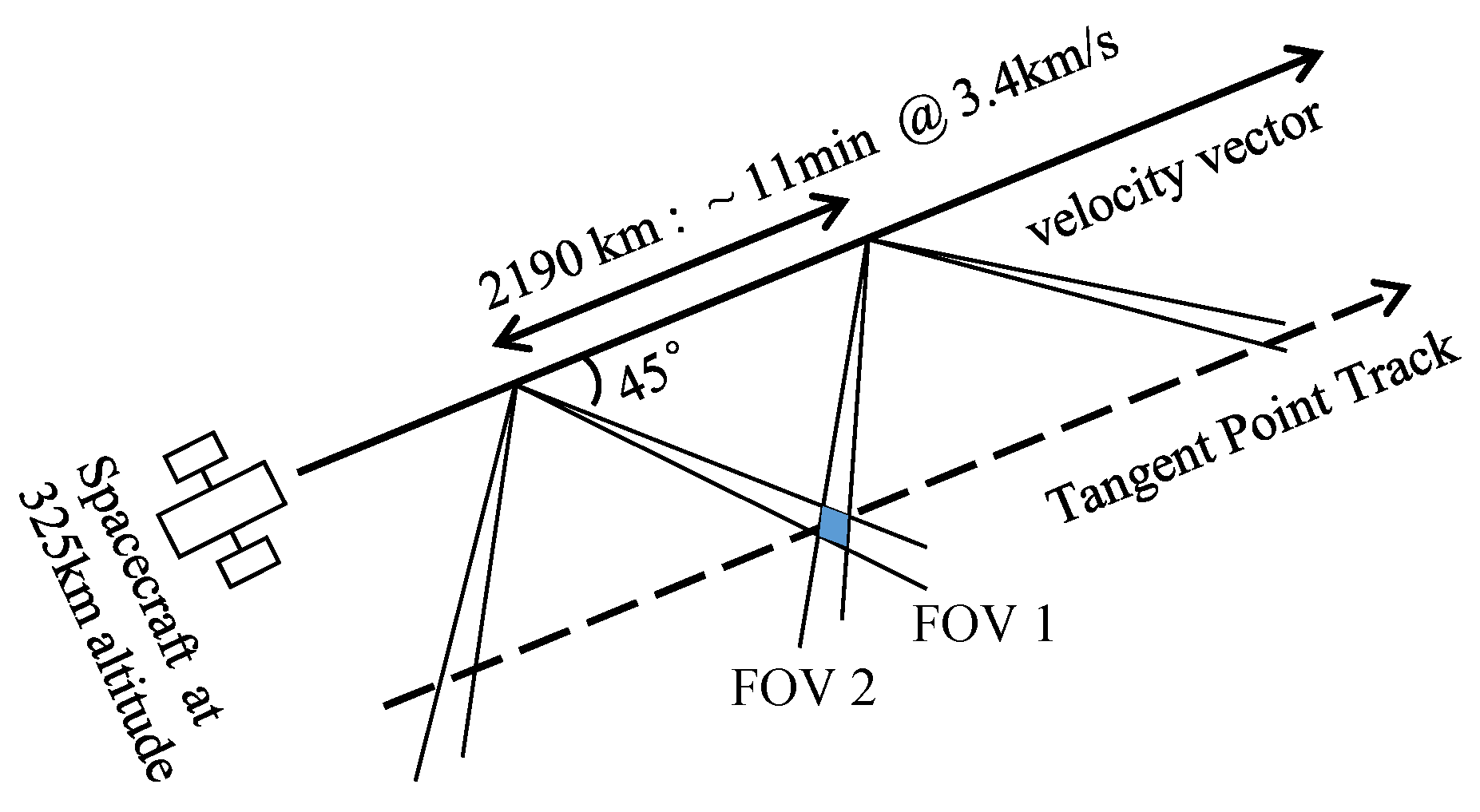
As shown in Figure 2, the instrument adopts a double field-of-view limb observation mode, with a satellite orbit height consistent with DYNAMO, which is 325 km [3]. The double field-of-view mode can measure line-of-sight wind fields in two orthogonal directions, and the limb observation can obtain vertical profiles of wind velocity. The parameters of the satellite orbit and instrument are summarized in

Table 2. Satellite and instrument parameters [3,10,24].

Parameters	Value
Mean satellite height	325 km
Orbit eccentricity (Elliptical orbit)	0.0072
Orbit inclination	70°
Azimuth of FOVs	FOV1: 45°, FOV2: 135°
Declination	21.75°
vertical resolution	1 km
Focal length of system	108 mm, F/2
Field of view	2° × 2°
Hor/Ver pixels of each FOV	125/125
Hor/Ver pixels per bin	5/5
The detected range of atmospheric altitude	10~60 km

. Based on the information provided above, we can calculate that the instrument’s field of view is 2° × 2°.

3.2. Selection of Instrument Optical Path Difference (OPD)

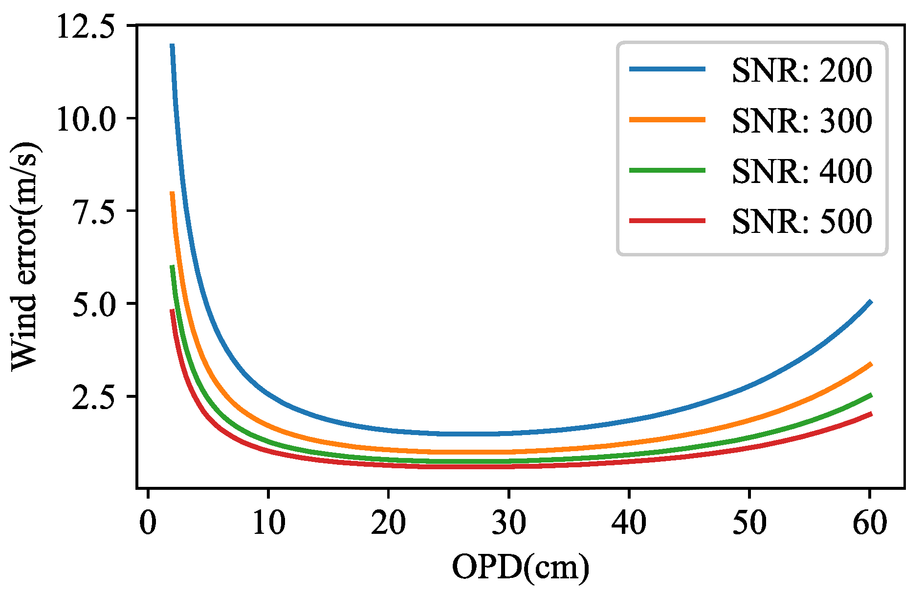
The wide-field Michelson interferometer used for wind field measurement is characterized by a large optical path difference (OPD) and high throughput. The OPD and the signal-to-noise ratio (SNR) of the instrument are closely related to the measurement accuracy of Martian wind velocity. To achieve high wind phase sensitivity, a large OPD is usually required. However, an excessively large OPD will lead to a rapid increase in instrument volume and weight, violating the goal of miniaturization and lightweight of the satellite-borne instrument. Therefore, a balance needs to be struck between the OPD and the wind velocity measurement accuracy. In ideal conditions, the phase step of the polarized wind imaging interferometer has been determined via calibration. Assuming the noise follows a Gaussian distribution, the measurement error of the wind velocity can be given by Equation (32), and the expected signal S can be estimated by Equation (33) [43,44]:

$${\sigma }_v=\frac{c{\lambda }_0}{2\sqrt{2}\pi UV(\mathrm{SNR})\mathsf{\Delta }}$$

(32)

$$S=\frac{I({\lambda }_0)}{4\pi }A{\mathsf{\Omega }}_{pixel}t\eta \delta t,$$

(33)

where ${\lambda }_0$ wavelength of target airglow emission line in nm, and Δ is OPD in cm. I is the atmospheric integrated emission rate in MR, A is the area of aperture stop of the optics in cm², ${\mathsf{\Omega }}_{pixel}$ is the solid angle subtended by each pixel on the detector, t is the overall transmittance of the optics, $\eta$ is the quantum efficiency of the CCD, and δt is the integration time in seconds(s).

The main CCD noise considered here includes dark current and readout noise. The SNR can be expressed as Equation (34):

$$\mathrm{SNR}=\frac{NS}{\sqrt{NS+N\ast Ds+{\mathsf{\eta }}_R{}^2}},$$

(34)

where N is the number of pixels in a bin, S is the pixel signal at the CCD (in electrons), Ds is the dark current signal per pixel of CCD (in electrons), ${\mathsf{\eta }}_{\mathrm{R}}$ is the readout noise of CCD, and the unit is electrons rms. The parameters related to the calculation of the SNR are shown in

Table 3. Related parameters for calculation of the SNR.

Symbols	Meaning	Value
c	Velocity of light	3 × 108 m/s
${\mathsf{\lambda }}_0$	Reference wavelength	1264.277 nm
U	Instrument visibility	0.9
V	Emission line visibility	Equation (27)
$\mathrm{I}({\mathsf{\lambda }}_0)$	Integrated emission rate	1~200 MR for dayglow
A	Aperture area	22.9 cm2
${\mathsf{\Omega }}_{bin}$	The solid angle subtended by each bin on the detector	3.83 × 10−7 sr
$\tau$	Optical system transmittance	0.15
$\eta$	CCD quantum efficiency	0.8
t	Integration time	10 s
N	The number of pixels in a bin	25
$\mathrm{Ds}$	Dark current signal per pixel of CCD	6 electrons
${\mathsf{\eta }}_{\mathrm{R}}$	Readout noise of CCD	40 electrons rms

.

Based on the wind velocity error equation given by Equation (32), Figure 3 depicts the variation of wind velocity error with optical path difference (OPD) and SNR. As seen from Figure 3, the relationship between wind velocity measurement error and interferometer optical path difference (OPD) is non-monotonic. With an increase in OPD, the wind error initially decreases and then increases. This behavior is primarily attributed to the decrease in instrument visibility resulting from the larger OPD. Additionally, it can be noted that an increase in SNR leads to a reduction in wind error. According to Equation (34) and the parameter values presented in Table 2, the estimated SNR of the designed polarized Martian wind imaging interferometer is above 480. Therefore, to ensure that the wind measurement error is less than 5 m/s with some margin, we have chosen a polarized Martian wind imaging interferometer with an OPD of 8.6 cm. According to Equation (27), the visibility of the emission spectral line is about 0.95, which is greater than 0.9 and represents an excellent value. Moreover, the phase variation caused by a wind velocity of 5 m/s is detectable, and its magnitude is not too small to be measured. This OPD is smaller than that of the DYNAMO instrument [3] and the 10 cm optical path difference designed for MWIMI [24], which also takes into account miniaturization and weight reduction.

3.3. All-Solid-State Arm Glass Compensation Design

Just like the compensation method used in reference [24,45], the compact all-solid-state Martian wind imaging interferometer needs to satisfy the requirements of large OPD, wide field widening, thermal compensation, and chromatic aberration correction. For the case of two-arm glass, these four conditions can be expressed as

$${\mathsf{\Delta }}_0=2n_1{d}_1-2n_2{d}_2$$

(35)

$$\frac{d_1}{n_1}-\frac{d_2}{n_2}=0$$

(36)

$$\frac{\partial {\mathsf{\Delta }}_0}{\partial T}=\frac{\partial }{\partial T}2{\displaystyle \sum _{j=1}^2{n}_j{d}_j=2}{\displaystyle \sum _{j=1}^2(n_j{d}_j{\alpha }_j+d_j{\beta }_j)}=0$$

(37)

$$\frac{\partial }{\partial \lambda }{\displaystyle \sum _{j=1}^2\frac{d_j}{n_j}=-}{\displaystyle \sum _{j=1}^2\frac{d_j}{n_j{}^2}}\frac{\partial n_j}{\partial \lambda }=0,$$

(38)

where n is the refractive index of the arm glass, d is the thickness of the arm glass, α represents the coefficient of thermal expansion, and β represents the refractive index temperature coefficient. The subscript j represents the number of the arm glass, and there are two arm glasses in our compact all-solid-state design, so j = 1, 2.

As the Martian wind imaging interferometer operates in a quasi-monochromatic mode, the achromatic condition represented by Equation (38) can be appropriately relaxed. Therefore, focusing on constructing the objective function based on Equations (35)–(37), the optimized glass pairs were selected from the glass library using the weighted least squares method. The final results are shown in

Table 4. Optimized combination results of arm glass.

Parameters	Glass 1	Glass 2
Glass	H-ZlaF2A	H-K8
Thickness (mm)	84.34	71.24
Refractive index @ 1264 nm	1.7792	1.5028

, where two types of CDGM glasses, H-ZlaF2A and H-K8, were chosen with thicknesses of 74.36 mm and 62.81 mm, respectively. The OPD of 8.6 mm was achieved with temperature variations within ±2 K, and the interference fringe shift was less than 0.01 cycle, indicating good temperature compensation performance. Within an incident angle of 6°, the difference between the center and edge orders in the interferogram was less than about one percent, indicating excellent wide-field performance of the design.

3.4. Design and Simulation of FP Etalon

To enhance the visibility of the polarized wind imaging interferogram, a combination of a narrowband filter and Fabry-Perot (FP) etalon is used to filter out the three spectral lines of O₂ 1.27 μm dayglow emission. Additionally, the combination also helps significantly reduce the strong solar background when observing the Martian atmosphere during the daytime. The design parameters of the narrowband filter and FP etalon are similar to those of the WAMI [10] and are shown in

Table 5. O₂ filter characteristics.

Filter	Bandwidth (nm)	Free Spectral Range (nm)
Narrowband Interference filter	2.0	None
F-P Etalon	0.1	2.0

. The technical specifications listed in Table 5 are established by considering the width of the three spectral lines in relation to the neighboring lines and taking into account the existing capabilities in narrow-band filter manufacturing.

The transmittance of the FP Etalon can be expressed by the Airy function, as a function of incident angle θ to the Etalon and the wavelength of the incident radiation, as shown in Equation (39).

$$T_{\mathrm{FP}}(\mathsf{\lambda },\mathsf{\theta })=\frac{1}{1+{\left(\frac{2F}{\mathsf{\pi }}\right)}^2{\sin }^2\left(\frac{2\mathsf{\pi }nd\cos (\mathsf{\theta })}{\mathsf{\lambda }}\right)}$$

(39)

where F is the finesse of the fringes, which is related to the reflectivity, d is the length of the etalon cavity, and θ is the angle of refraction inside the cavity.

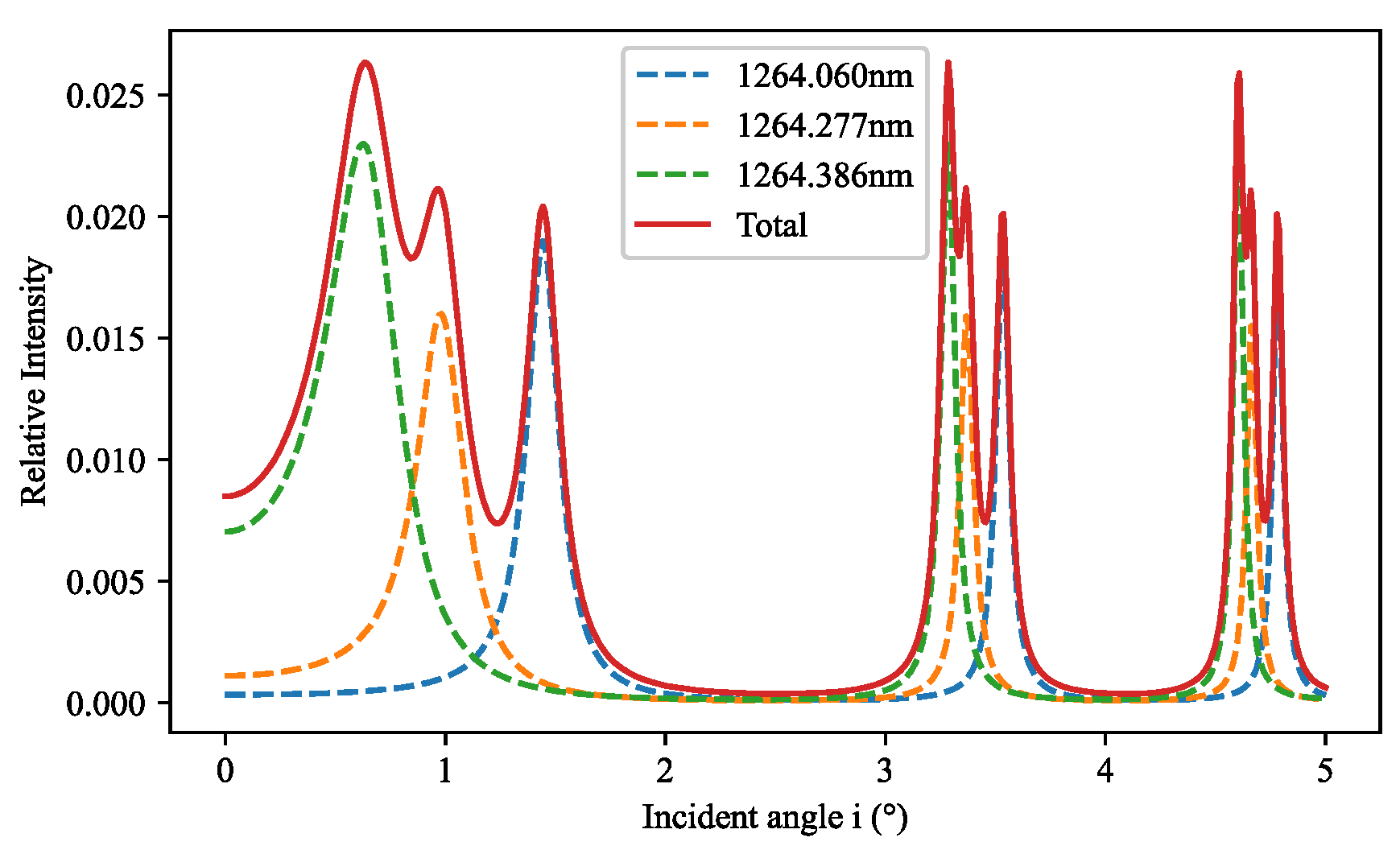
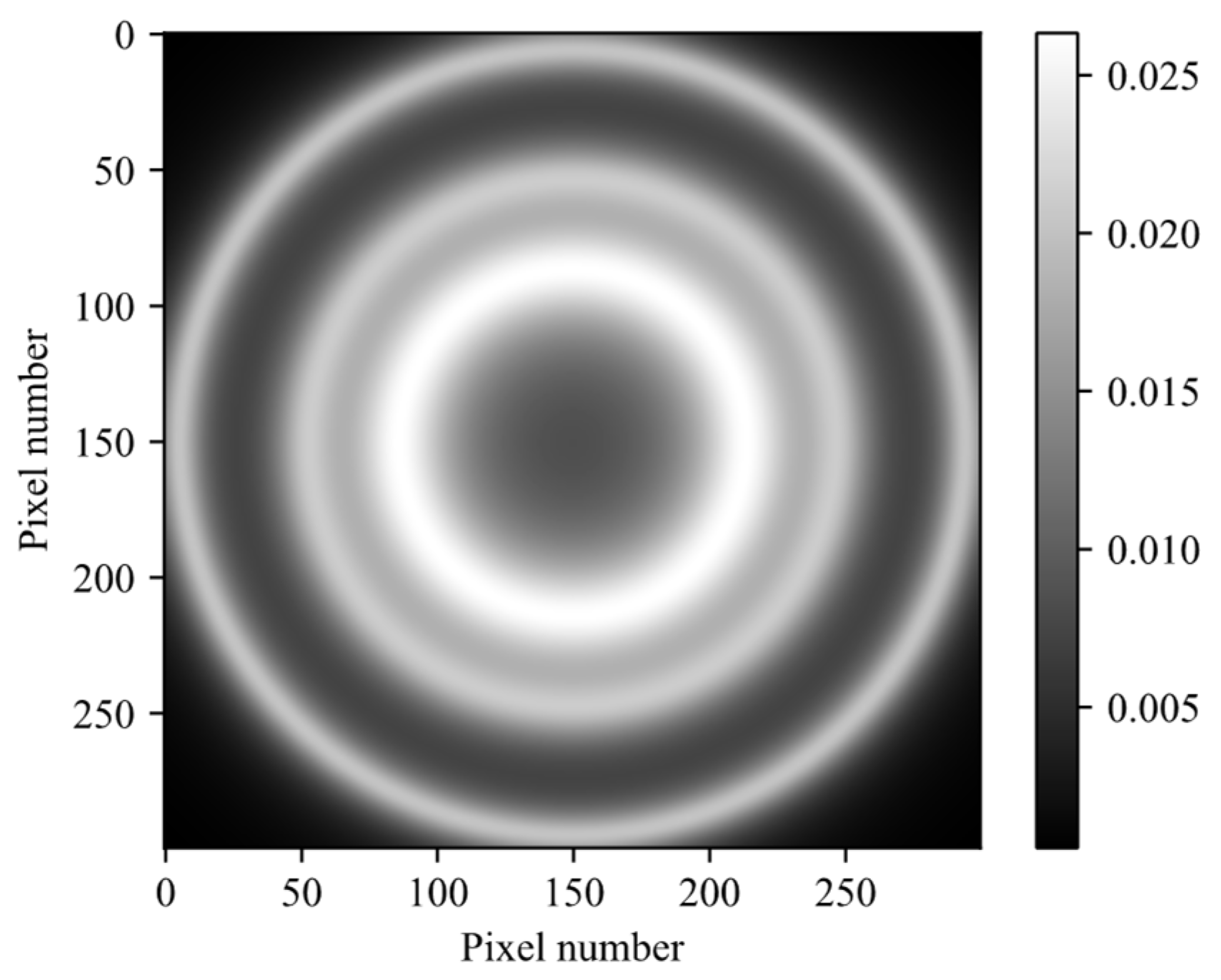
The F-P Etalon was designed for Mars wind field imaging, using fused quartz as the mirror material and air as the medium. The air gap thickness was approximately 399.45 μm, with an interference order of 632, and a diameter of approximately 50 mm, with a fringe finesse of 20. The selection of these parameters aligns with the current state of processing and manufacturing capabilities and also complies with the technical specifications outlined in Table 5. The designed F-P Etalon achieves a high transmittance of over 99.5% for all three O₂ dayglow spectral lines, as depicted in Figure 4, taking into account the relative intensity of the three spectral lines in Table 1. In Figure 4, the dashed line represents the relative intensity of the three spectral lines individually, while the solid line represents the total relative intensity of the lines. The simulated image of the three O₂ spectral lines within the instrument’s field of view using Python is shown in Figure 5, with three circular rings corresponding to the three independent dayglow spectral lines. It should be noted that narrowband interference filters and the F-P etalons have strong temperature dependence. Temperature can cause changes in the optical path of the filter, resulting in wavelength drift of the transmitted airglow spectrum and affecting the filter transmittance. Therefore, on the one hand, when selecting and fabricating filters, materials with low thermal expansion coefficients, such as fused quartz, should be chosen as the substrate material. On the other hand, the temperature of the instrument’s environment should be strictly controlled. As a spaceborne payload, temperature should be controlled with an accuracy of about 0.01 K.

3.5. Pyramid Prism

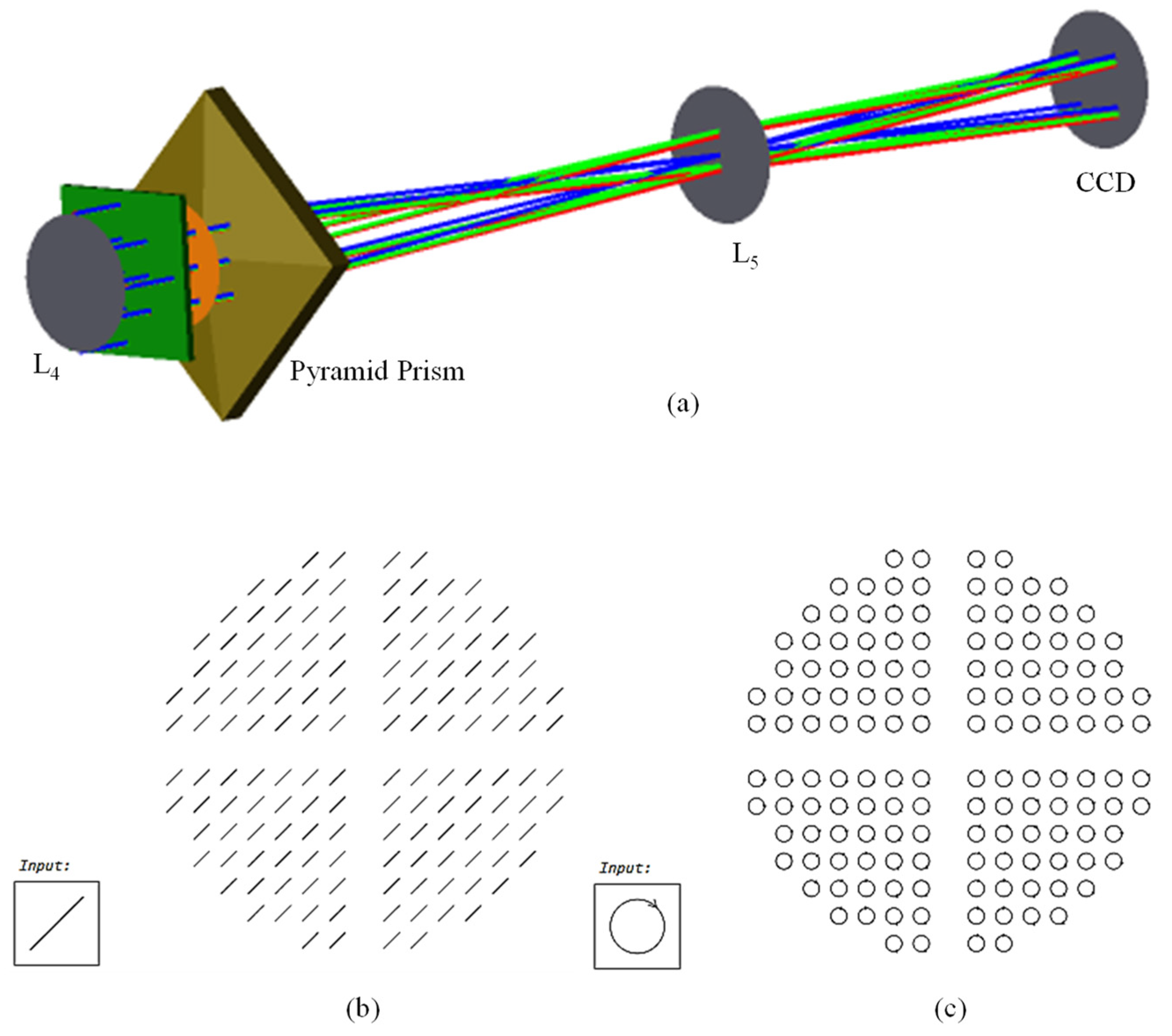
The pyramid prism plays a pivotal role in enabling the four-step phase-shift static modulation for polarized Martian wind imaging interferometry. Its top-down perspective is depicted in Figure 6. Its primary function lies in segmenting the aperture into four distinct areas, with each of the four faces aligning with the corresponding sub-faces of P₂. This harmonious alignment facilitates the execution of a four-step phase-shift process, essential for generating wind field interferograms. The designed pyramid prism has a wedge angle of approximately 5.7°, which can be effectively treated as an optical wedge. Given the instrument’s narrow field of view of around 2°, it can be deduced from the Fresnel equations that the alteration in the polarization state of the transmitted light through the pyramid prism is negligible and can be disregarded. We utilized Zemax optics software to trace the polarization pupil map of collimated light after passing through the pyramid prism, as depicted in Figure 6. Figure 6a illustrates the optical layout, while Figure 6b,c respectively, display the polarization distribution on the image plane for 45° linearly polarized light and right-circularly polarized light passing through the pyramid prism. It can be observed that the image plane is divided into four sub-regions by the pyramid prism, and the polarization state of the incident and transmitted light remains consistent.

3.6. Wind Field Measurement Simulation

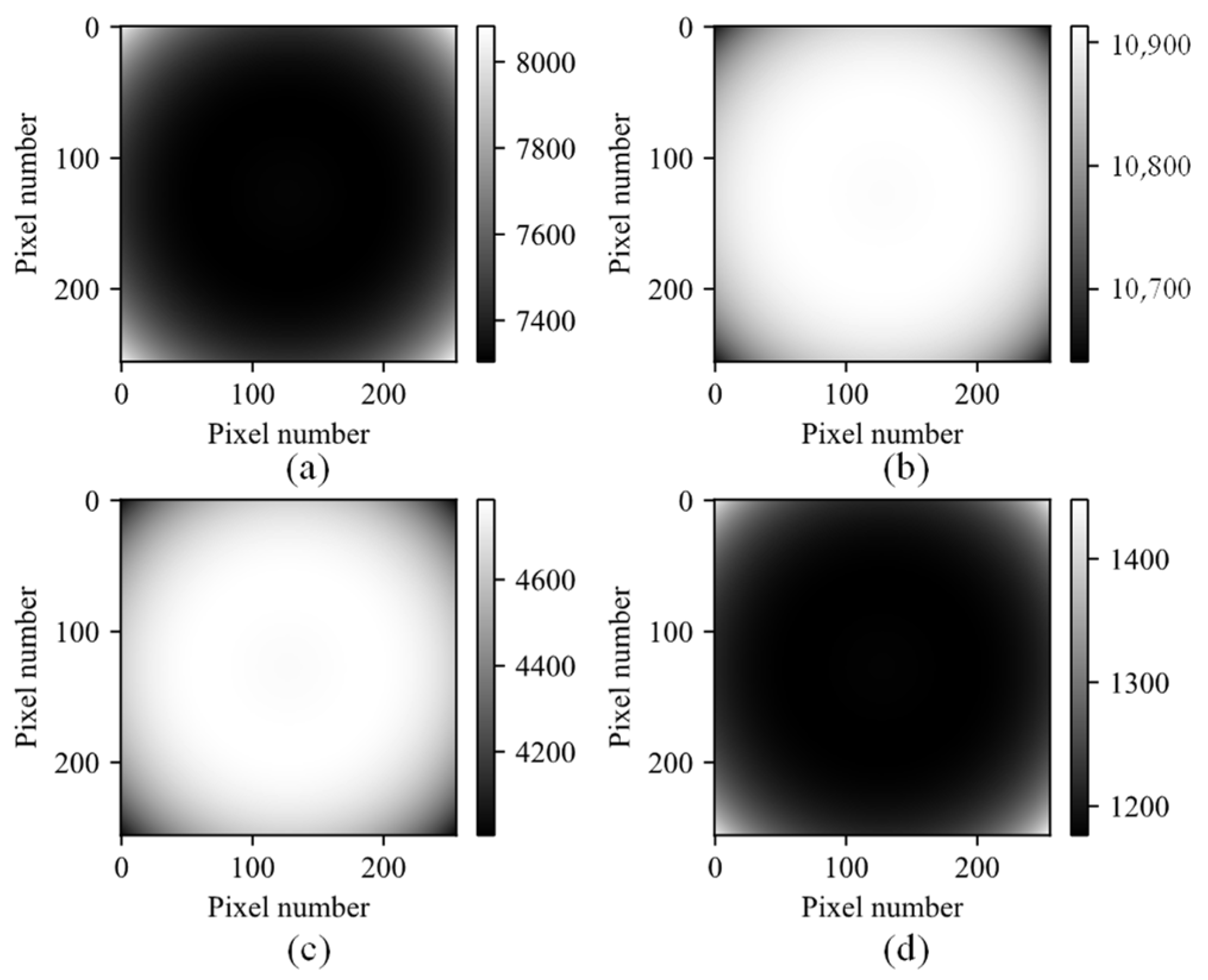
Based on the designed parameters, we conducted simulations on the wide-field performance and wind velocity inversion of the compact polarized Martian wind imaging interferometer. We used a 14-bit CCD detector with an effective pixel count of 512 × 512. Following the static four-quadrant polarization modulation principle, each sub-image has a size of 256 × 256 and a pixel size of 15 μm. We used 5 × 5 pixel binning. The interferometer uses the two arm glasses from Table 4 to achieve an OPD of about 8.6 cm. To observe the wide-field effect, we simulated the interferogram without wind velocity or “zero wind velocity” and observed the four sub-images with phase steps of 0°, 90°, 180°, and 270°, as shown in Figure 7. The gray values of each sub-image have a significant difference due to the phase steps, but the gray value variation range of each sub-image is small from its center to margin, indicating excellent wide-field performance.

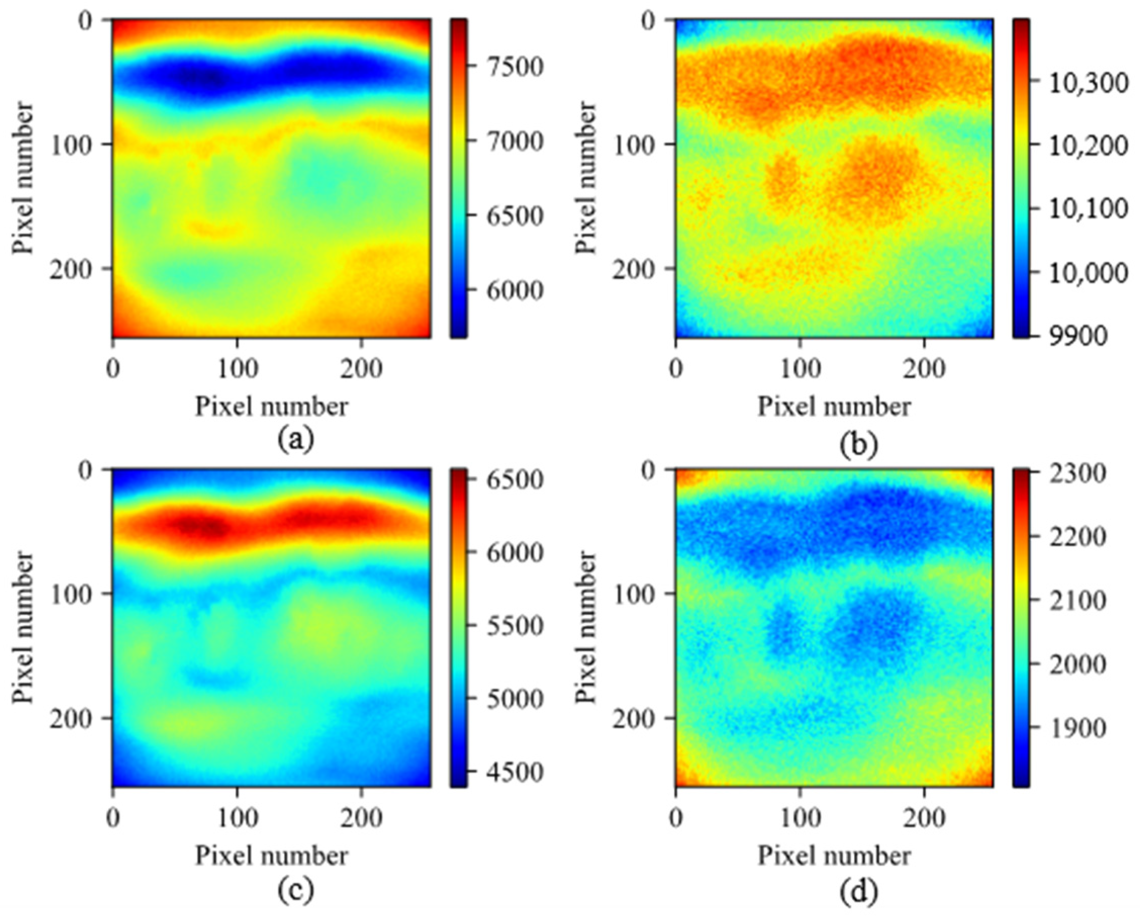
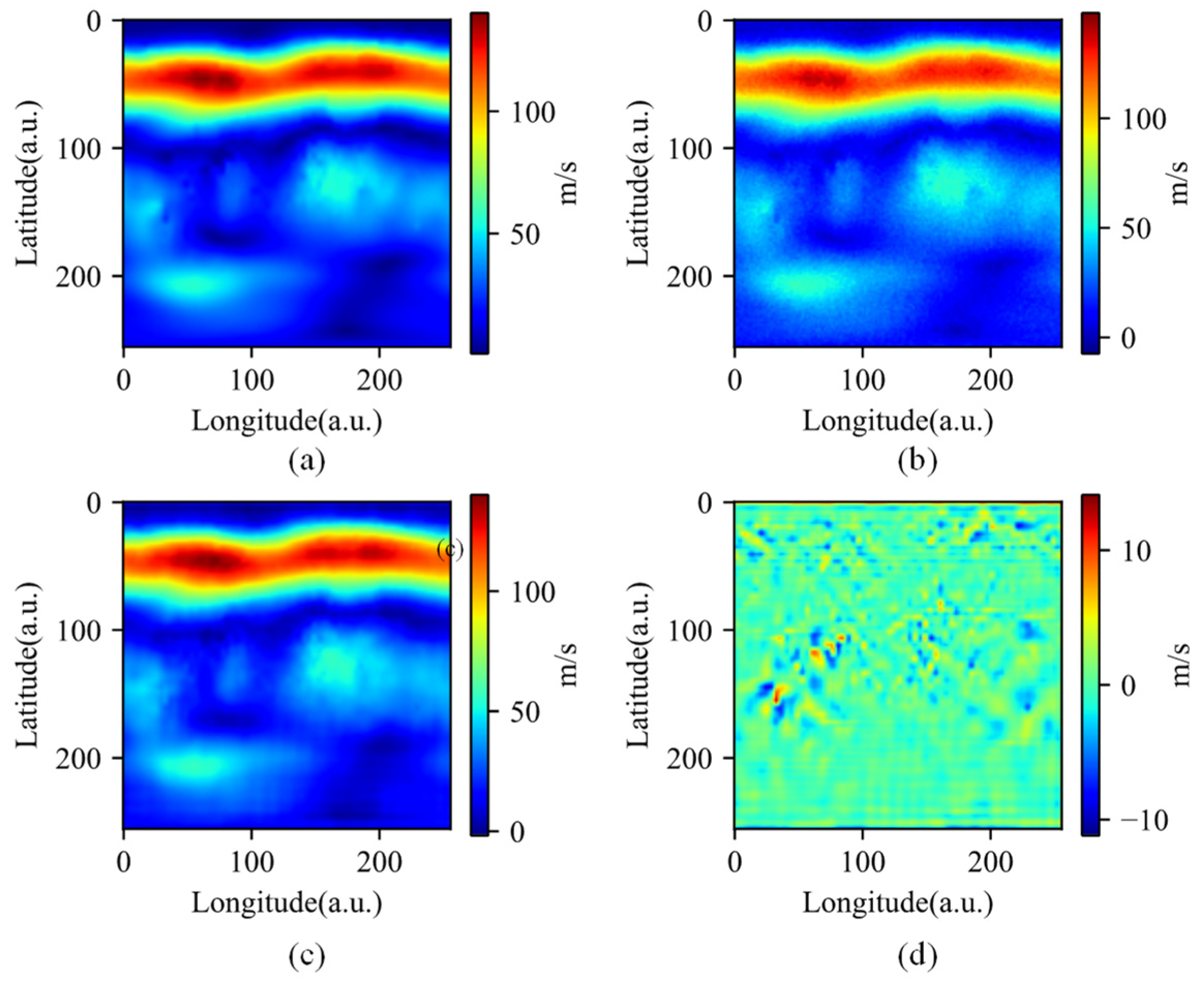
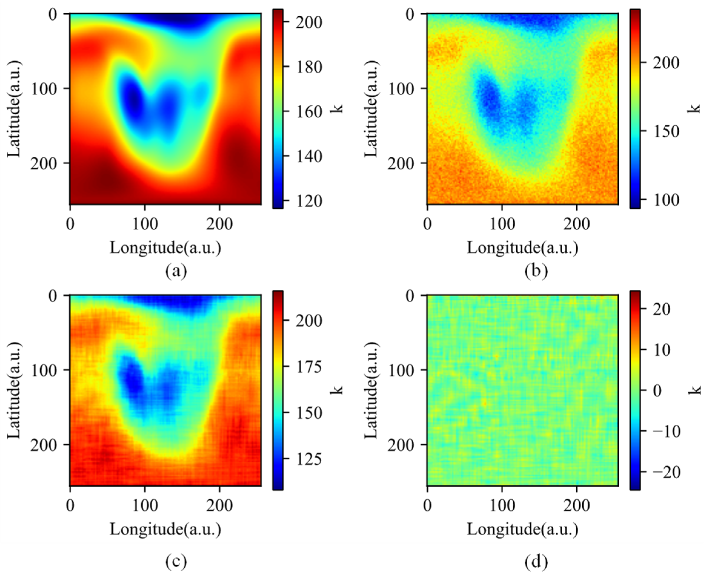
Using the typical Martian atmospheric wind and temperature from the MCD Martian atmospheric model [46] and the polarized wind imaging interferogram model represented by Equation (19), simulated Martian wind imaging interferograms were generated. The solar longitude is approximately 65°, the local time is 0:00 h, and the altitude is around 30 km. To simulate various types of noise present in real scenarios, such as detector readout noise, Gaussian noise was added to the four interferograms. Four interferograms were augmented with the same Gaussian noise, with a standard deviation of around 92 in pixel grayscale value. Based on the interferogram with the lowest average pixel intensity, which is approximately 2000, the calculated signal-to-noise ratio (SNR) of the interferograms is approximately 472. This aligns with the SNR derived from Equation (34) and the analysis in Figure 3. As shown in Figure 8, different sub-images have different intensities, reflecting their distinct interference phases. As shown in Figure 9, (a) represents a typical wind velocity map of the Martian atmosphere, (b) shows the wind velocity map directly derived from interferograms with noise, (c) displays the wind velocity map retrieved from denoised interferograms, and (d) is wind velocity inversion error. The denoising method used is a neural network-based approach developed by the authors in a previous publication [47], which enables fast denoising of the wind imaging interferograms. From Figure 9, it can be observed that denoising the interferograms significantly reduces the wind velocity inversion error. Through calculations, the root mean square (RMS) wind velocity error from directly inverting the noisy interferograms is approximately 3.39 m/s. After denoising the interferograms, the RMS wind velocity error from the inversion is approximately 1.78 m/s. This demonstrates the significant impact of denoising on wind velocity inversion. Similarly, utilizing the relationship between temperature and interferograms expressed in Equation (27), we perform temperature inversion for typical Martian atmospheric temperature field [46]. As shown in Figure 10, (a) represents a typical temperature distribution map of the Martian atmosphere, (b) shows the temperature map directly retrieved from interferograms with noise, (c) displays the temperature map retrieved from denoised interferograms, and (d) is temperature inversion error. Through calculations, denoising the interferograms improves the RMS of temperature inversion error from 9.16 K to 2.79 K, indicating the significance of interferogram denoising in temperature inversion. The validation of wind velocity and temperature inversion demonstrates the feasibility of the proposed polarized Martian atmospheric wind imaging interferometer scheme.

4. Discussion

The polarized, all-solid-state, dual-layer compensating medium interferometer proposed in this paper presents a compact solution for static wind field measurement on Mars. We have chosen the three spectral lines of O₂ dayglow in the Martian atmosphere as our observation source. By optimizing the interferometer’s optical path difference (OPD) and conducting preliminary forward and inverse simulations, we have validated the measurement accuracy of wind velocity and temperature. Certainly, as illustrated in Figure 3, there is still potential for reducing the OPD. While this could result in a diminished sensitivity in wind phase measurement, the substantial decrease in the OPD holds paramount importance for achieving instrument compactness and weight reduction. Furthermore, the incorporation of novel technologies such as freeform surfaces could replace the telescope and imaging systems in the optics. This would further reduce the instrument’s overall size and weight, aligning with the compact and lightweight demands of Mars-bound payloads. Additionally, advanced data inversion algorithms, such as those based on deep learning networks, could be employed for wind velocity and temperature inversion. This approach has the potential to enhance computational speed and precision, thereby fostering a comprehensive improvement in the overall system.

In Section 3.6, we employed typical Martian atmospheric wind velocity and temperatures in conjunction with the designed parameters of the polarized Martian wind imaging interferometer. We utilized a straightforward “Four-intensity method” to validate the interferometer’s capability to retrieve wind velocity and temperatures. It should be noted that in practice, obtaining vertical profiles of wind velocity and temperature requires the integration of orbital models, instrument models, Martian atmospheric models, forward modeling, and complex inversion algorithms. Furthermore, we confirmed that appropriate noise reduction is highly effective in enhancing the precision of wind velocity and temperature retrieval. We also observed that the denoising effectiveness is dependent on the estimation of the noise level.

The proposed polarized interferometric scheme in this study offers not only advantages such as low stray light, cost-effectiveness, and simple phase modulation; it also holds the potential to exploit the polarization characteristics of Martian atmospheric airglow radiation. When combined with polarization calibration techniques, it opens up avenues to probe the polarimetric properties of the Martian atmosphere.

5. Conclusions

This paper presents a compact, all-solid-state, static, and miniaturized design of a polarized interferometer for Martian atmospheric wind field measurement. All components of the interferometer are securely bonded together to form a robust unit. By analyzing the signal-to-noise ratio (SNR), an optical path difference (OPD) of 8.6 cm is selected, and a two-arm-glass configuration is chosen as the compensating glass to achieve wide field of view, high throughput, temperature compensation, and miniaturization. An F-P Etalon is designed to selectively filter out the three spectral lines of O₂ (a¹Δ_g) at 1.27 μm dayglow. Through theoretical analysis, formula derivation, and computer simulations, we have arrived at the following conclusions:

• The proposed compact polarized solid-state Mars wind imaging interferometer scheme is capable of high-precision Mars wind field measurement. An OPD of 8.6 cm can achieve a measurement accuracy of 5 m/s for Martian atmospheric wind velocity and 5 K for temperature measurement, as validated through theoretical analysis and simulations.
• The designed pyramid prism with a wedge angle of 5.7° has a negligible impact on the polarization state of the incident light, making it suitable for aperture segmentation in the polarized Mars wind imaging interferometer.
• Denoising of the wind field interferogram is necessary and can further enhance the accuracy of detecting Mars atmospheric wind veloctiy and temperature.

This miniaturized design offers excellent stability and combines static operation, compact size, and cost-effectiveness. Furthermore, it effectively mitigates the issue of stray light caused by light returning from the interferometer towards the light source direction. The proposed approach provides valuable insights for the development of Martian atmospheric wind imaging interferometers and contribute to the unique dataset for investigating Martian atmospheric dynamics. This will enhance our understanding of Martian atmospheric circulation, atmospheric gravity waves, and other wave phenomena, as well as the characteristics of constituent transport and even the evolution of Mars’ climate. It establishes the theoretical and technological groundwork for future simultaneous measurement of Martian atmospheric wind fields, temperature fields, and ozone concentrations from spacecraft in a static manner. It enables comprehensive predictions of the Martian atmospheric environment for spacecraft and provides crucial technical support for human Mars exploration missions.

References

- Yang, N.; Xia, C.; Yu, T.; Zuo, X.; Sun, Y.; Yan, X.; Zhang, J.; Wang, J.; Le, H.; Liu, L.; et al. Measurement of Martian atmospheric winds by the O2 1.27 μm airglow observations using Doppler Michelson Interferometry: A concept study. Sci. China Earth Sci. 2021, 64, 2027–2042. [Google Scholar] [CrossRef]
- Read, W.G.; Tamppari, L.K.; Livesey, N.J.; Clancy, R.T.; Forget, F.; Hartogh, P.; Rafkin, S.C.R.; Chattopadhyay, G. Retrieval of wind, temperature, water vapor and other trace constituents in the Martian Atmosphere. Planet. Space Sci. 2018, 161, 26–40. [Google Scholar] [CrossRef]
- Ward, W.E.; Gault, W.A.; Rowlands, N.; Wang, S.; Shepherd, G.G.; Mcdade, I.C.; McConnell, J.C.; Michelangeli, D.V.; Caldwell, J.J. An imaging interferometer for satellite observations of wind and temperature on Mars, the Dynamic Atmosphere Mars Observer (DYNAMO). In Proceedings of the Applications of Photonic Technology, Quebec City, QC, Canada, 17 February 2003. [Google Scholar] [CrossRef]
- Muhleman, D.O.; Clancy, R.T. Microwave spectroscopy of the Mars atmosphere. Appl. Opt. 1995, 34, 6067–6080. [Google Scholar] [CrossRef] [PubMed]
- Kasai, Y.; Sagawa, H.; Kuroda, T.; Manabe, T.; Ochiai, S.; Kikuchi, K.-I.; Nishibori, T.; Baron, P.; Mendrok, J.; Hartogh, P.; et al. Overview of the Martian atmospheric submillimetre sounder FIRE. Planet. Space Sci. 2012, 63–64, 62–82. [Google Scholar] [CrossRef]
- Hays, P.B.; Abreu, V.J.; Dobbs, M.E.; Gell, D.A.; Grassl, H.J.; Skinner, W.R. The high-resolution Doppler imager on the Upper Atmosphere Research Satellite. J. Geophys. Res. 1993, 98, 10713–10723. [Google Scholar] [CrossRef]
- Shepherd, G.G.; Thuillier, G.; Gault, W.A.; Solheim, B.H.; Hersom, C.; Alunni, J.M.; Brun, J.-F.; Brune, S.; Charlot, P.; Cogger, L.L. WINDII, the wind imaging interferometer on the Upper Atmosphere Research Satellite. J. Geophys. Res. Atmos. 1993, 98, 10725–10750. [Google Scholar] [CrossRef]
- Gault, W.A.; Shepherd, G.G.; Thuillier, G.; Solheim, B.H.; Hersom, C.H.; Brun, J.-F.; Brune, S.; Gore, J. WIND Imaging Interferometer (WINDII) on the upper-atmosphere research satellite. In Proceedings of the Instrumentation for Planetary and Terrestrial Atmospheric Remote Sensing, San Diego, CA, USA, 29 June 1992; Volume 1745. [Google Scholar]
- Bird, J.C.; Liang, F.; Solheim, B.H.; Shepherd, G.G. A polarizing Michelson interferometer for measuring thermospheric winds. Meas. Sci. Technol. 1995, 6, 1368–1378. [Google Scholar] [CrossRef]
- Gault, W.A.; Brown, S.; Moise, A.; Liang, D.; Sellar, G.; Shepherd, G.G.; Wimperis, J. ERWIN: An E-region wind interferometer. Appl. Opt. 1996, 35, 2913–2922. [Google Scholar] [CrossRef]
- Gault, W.A.; Mcdade, I.C.; Shepherd, G.G.; Mani, R.; Brown, S.; Gregory, P.; Scott, A.; Rochon, Y.J.; Evans, W.F.J. SWIFT: An infrared Doppler Michelson interferometer for measuring stratospheric winds. In Proceedings of the Sensors, Systems, and Next-Generation Satellites V, Toulouse, France, 12 December 2001; SPIE: New York, NY, USA, 2001; pp. 476–481. [Google Scholar]
- Ward, W.E.; Gault, W.A.; Shepherd, G.G.; Rowlands, N. The Waves Michelson interferometer: A visible/near-IR interferometer for observing middle atmosphere dynamics and constituents. In Proceedings of the Sensors, Systems, and Next-Generation Satellites V, Toulouse, France, 12 December 2001; SPIE: New York, NY, USA, 2001; pp. 100–111. [Google Scholar]
- Kristoffersen, S.K.; Ward, W.E.; Langille, J.; Gault, W.A.; Power, A.; Miller, I.; Scott, A.; Arsenault, D.; Favier, M.; Losier, V.; et al. Wind imaging using simultaneous fringe sampling with field-widened Michelson interferometers. Appl. Opt. 2022, 61, 6627–6641. [Google Scholar] [CrossRef]
- Babcock, D.D. Mesospheric Imaging Michelson Interferometer Instrument Development and Observations. Ph.D. Thesis, York University, Toronto, Canada, 2006. [Google Scholar]
- Langille, J.A. The Michelson Interferometer for Airglow Dynamics Imaging: Implementation, Characterzation and Testing. Ph.D. Thesis, University of New Brunswick, Fredericton, Canada, 2010. [Google Scholar]
- Yan, T.; Langille, J.A.; Ward, W.E.; Gault, W.A.; Scott, A.; Bell, A.; Touahiri, D.; Zheng, S.H.; Zhang, C. A compact static birefringent interferometer for the measurement of upper atmospheric winds: Concept, design and lab performance. Atmos. Meas. Tech. 2021, 14, 6213–6232. [Google Scholar] [CrossRef]
- Ortland, D.A.; Hays, P.B.; Skinner, W.R.; Yee, J.-H. Remote sensing of mesospheric temperature and O2(1Σ) band volume emission rates with the high-resolution Doppler imager. J. Geophys. Res. Atmos. 1998, 103, 1821–1835. [Google Scholar] [CrossRef]
- Shi, D. Research on the Data Retrieval and Calibration of the Upper Atmosphere Wind and Temperature Measuring Fabry-Perot Interferometer. Ph.D. Thesis, University of Chinese Academy of Sciences, Xi’an, China, 2015. [Google Scholar]
- Killeen, T.; Wu, Q.; Solomon, S.; Ortland, D.; Skinner, W.; Niciejewski, R.; Gell, D. TIMED Doppler Interferometer: Overview and recent results. J. Geophys. Res. Space Phys. 2006, 111, A10S01. [Google Scholar] [CrossRef]
- Englert, C.R.; Babcock, D.D.; Harlander, J.M. Doppler asymmetric spatial heterodyne spectroscopy (DASH): Concept and experimental demonstration. Appl. Opt. 2007, 46, 7297–7307. [Google Scholar] [CrossRef]
- Yang, X.; Feng, Y.; Wen, Z.; Di, F. Doppler Asymmetric Spatial Heterodyne Interferometry for Wind Measurement in Middle and Upper Atmosphere (Invited). Acta Photonica Sin. 2022, 51, 0851516. [Google Scholar]
- Englert, C.R.; Harlander, J.M.; Brown, C.M.; Marr, K.D.; Miller, I.J.; Stump, J.E.; Hancock, J.; Peterson, J.Q.; Kumler, J.; Morrow, W.H.; et al. Michelson Interferometer for Global High-Resolution Thermospheric Imaging (MIGHTI): Instrument Design and Calibration. Space Sci. Rev. 2017, 212, 553–584. [Google Scholar] [CrossRef]
- Harding, B.J.; Chau, J.L.; He, M.; Englert, C.R.; Harlander, J.M.; Marr, K.D.; Makela, J.J.; Clahsen, M.; Li, G.; Ratnam, M.V.; et al. Validation of ICON-MIGHTI Thermospheric Wind Observations: 2. Green-Line Comparisons to Specular Meteor Radars. J. Geophys. Res. Space Phys. 2021, 126, e2020JA028947. [Google Scholar] [CrossRef]
- Rong, P.; Zhang, C.; Ward, W.E.; Zhu, H.; Dai, H. Compensation optimization for a static Mars wind imaging Michelson interferometer. Opt. Lasers Eng. 2021, 142, 106589. [Google Scholar] [CrossRef]
- Zhang, C.; Yan, T.; Mu, T.; He, Y. Theoretical Model and Design of A Novel Static Polarization Wind Imaging Interferometer (NSPWII). ISPRS Ann. Photogramm. Remote Sens. Spat. Inf. Sci. 2020, V-1-2020, 383–388. [Google Scholar] [CrossRef]
- Zhang, C.; Yan, T.; Wang, Y.; Zhang, B.; Chen, Z.; Chen, Z.; Ward, W.; Kristoffersen, S. Static wind imaging Michelson interferometer for the measurement of stratospheric wind fields. Opt. Express 2023, 31, 29411–29426. [Google Scholar] [CrossRef]
- Noxon, J.F.; Traub, W.A.; Carleton, N.P.; Connes, P. Detection of O2 dayglow emission from Mars and the Martian ozone abundance. Astron. J. 1976, 207, 1025–1035. [Google Scholar] [CrossRef]
- Krasnopolsky, V.A. Mapping of Mars O2 1.27 μm dayglow at four seasonal points. Icarus 2003, 165, 315–325. [Google Scholar] [CrossRef]
- Krasnopolsky, V.A. Photochemistry of the martian atmosphere: Seasonal, latitudinal, and diurnal variations. Icarus 2006, 185, 153–170. [Google Scholar] [CrossRef]
- Krasnopolsky, V.A. Seasonal variations of photochemical tracers at low and middle latitudes on Mars: Observations and models. Icarus 2009, 201, 564–569. [Google Scholar] [CrossRef]
- Guslyakova, S.; Fedorova, A.A.; Lefèvre, F.; Korablev, O.I.; Montmessin, F.; Bertaux, J.L. O2(a1Δg) dayglow limb observations on Mars by SPICAM IR on Mars-Express and connection to water vapor distribution. Icarus 2014, 239, 131–140. [Google Scholar] [CrossRef]
- Fedorova, A.; Korablev, O.; Perrier, S.; Bertaux, J.-L.; Lefevre, F.; Rodin, A. Observation of O2 1.27 μm dayglow by SPICAM IR: Seasonal distribution for the first Martian year of Mars Express. J. Geophys. Res. 2006, 111, E09S07. [Google Scholar] [CrossRef]
- Altieri, F.; Zasova, L.V.; D’aversa, E.; Bellucci, G.; Carrozzo, F.G.; Gondet, B.; Bibring, J.P. O2 1.27 μm emission maps as derived from OMEGA/MEx data. Icarus 2009, 204, 499–511. [Google Scholar] [CrossRef]
- Fedorova, A.A.; Lefèvre, F.; Guslyakova, S.; Korablev, O.; Bertaux, J.L.; Montmessin, F.; Reberac, A.; Gondet, B. The O2 nightglow in the martian atmosphere by SPICAM onboard of Mars-Express. Icarus 2012, 219, 596–608. [Google Scholar] [CrossRef]
- Bertaux, J.L.; Gondet, B.; Lefèvre, F.; Bibring, J.P.; Montmessin, F. First detection of O2 1.27 μm nightglow emission at Mars with OMEGA/MEX and comparison with general circulation model predictions. J. Geophys. Res. 2012, 117, E00J04. [Google Scholar] [CrossRef]
- Guslyakova, S.; Fedorova, A.; Lefèvre, F.; Korablev, O.; Montmessin, F.; Trokhimovskiy, A.; Bertaux, J.L. Long-term nadir observations of the O2 dayglow by SPICAM IR. Planet. Space Sci. 2016, 122, 1–12. [Google Scholar] [CrossRef]
- Krasnopolsky, V.A. Photochemical mapping of Mars. J. Geophys. Res. Planets 1997, 102, 13313–13320. [Google Scholar] [CrossRef]
- Todd Clancy, R.; Smith, M.D.; Lefèvre, F.; McConnochie, T.H.; Sandor, B.J.; Wolff, M.J.; Lee, S.W.; Murchie, S.L.; Toigo, A.D.; Nair, H.; et al. Vertical profiles of Mars 1.27 µm O2 dayglow from MRO CRISM limb spectra: Seasonal/global behaviors, comparisons to LMDGCM simulations, and a global definition for Mars water vapor profiles. Icarus 2017, 293, 132–156. [Google Scholar] [CrossRef]
- Wu, K.; Fu, D.; Feng, Y.; Li, J.; Hao, X.; Li, F. Simulation and application of the emission line O19P18 of O2(a1Δg) dayglow near 1.27 μm for wind observations from limb-viewing satellites. Opt. Express 2018, 26, 16984–16999. [Google Scholar] [CrossRef] [PubMed]
- Krasnopolsky, V.A. Spectroscopy and Photochemistry of Planetary Atmospheres and Ionospheres: Mars, Venus, Titan, Triton and Pluto; Cambridge University Press: Cambridge, UK, 2019; Volume 23. [Google Scholar]
- Crisp, D.; Meadows, V.S.; Bézard, B.; Bergh, C.d.; Maillard, J.P.; Mills, F.P. Ground-based near-infrared observations of the Venus nightside: 1.27-μm O2(a1Δg) airglow from the upper atmosphere. J. Geophys. Res. 1996, 101, 4577–4593. [Google Scholar] [CrossRef]
- Wang, Y.; Zhang, C.; Rong, P.; Yan, T.; Chen, Z. Influence of the tilted arm glass on the temperature and wind velocity inversion for a static wind imaging interferometer. Opt. Commun. 2021, 495, 127118. [Google Scholar] [CrossRef]
- Ward, W.E. The Design and Implementation of the Wide-Angle Michelson Interferometer to Observe Thermospheric Winds. Ph.D. Thesis, York University, Toronto, Canada, 1988. [Google Scholar]
- Langille, J.A.; Ward, W.E.; Scott, A.; Arsenault, D.L. Measurement of two-dimensional Doppler wind fields using a field widened Michelson interferometer. Appl. Opt. 2013, 52, 1617–1628. [Google Scholar] [CrossRef]
- Thuillier, G.; Shepherd, G.G. Fully compensated Michelson interferometer of fixed-pathdifference. Appl. Opt. 1985, 24, 1599–1603. [Google Scholar] [CrossRef]
- Millour, E.; Forget, F.; Spiga, A.; Vals, M.; Zakharov, V.; Navarro, T.; Montabone, L.; Lefevre, F.; Montmessin, F.; Chaufray, J.-Y.; et al. The Mars Climate Database (MCD Version 5.3). In Proceedings of the 19th EGU General Assembly, Vienna, Austria, 23–28 April 2017; EGU: Munich, Germany, 2017; p. 12247. [Google Scholar]
- Wang, Y.; Zhang, C.; Chen, Z.; Sun, Y.; Zhang, P. Measurement of visibility and phase steps of a static wind imaging interferometer assisted by deep learning. Appl. Opt. 2022, 61, 3533–3541. [Google Scholar] [CrossRef] [PubMed]
Figure 1.
Schematic diagram of polarized Martian wind imaging interferometer. P1 represents a linear polarizer, and the red arrow indicates that its transmission axis is at a 45° angle to the x-axis. P2 refers to an array of linear polarizers, consisting of four sub-linear polarizers with their transmission axes at angles of 0°, 45°, 90°, and 135° relative to the x-axis, respectively.
Figure 2.
Limb imaging geometry (from the orbit) [3].
Figure 3.
Wind velocity error variations with OPD and SNR.
Figure 4.
Relative intensity of F-P etalon as a function of the incident angle for the three O2 spectral lines. The three dashed lines represent the relative intensities of the three selected dayglow spectral lines used for Mars atmospheric wind field measurement after passing through the F-P Etalon. The solid line represents the total intensity or the envelope line of these three spectral lines.
Figure 5.
Simulated image of O2 three spectral lines within the instrument’s field of view. The three circular rings correspond to the selected three independent dayglow lines.
Figure 6.
The ray tracing of pyramid prism modeled using Zemax optics software: (a) the optical layout; (b) the polarization pupil map for 45° linearly polarization incidence; (c) the polarization pupil map for circularly polarized incidence.
Figure 7.
Simulated interferograms with the standard “Four-phase step” for zero wind velocity on the CCD detector. The phase steps are (a) 0°, (b) 90°, (c) 180°, and (d) 270°, respectively. The grayscale values are relative units, and the CCD is a 12-bit gray level.
Figure 8.
Simulated interferograms of the Martian wind field with the standard “Four-phase step” on CCD detector. The phase steps are (a) 0°, (b) 90°, (c) 180°, and (d) 270°, respectively.
Figure 9.
Martian atmospheric wind velocity images. (a) Typical original Martian wind velocity image (the solar longitude is approximately 65°, the local time is 0:00 h, the altitude is around 30 km, and presence of dust is not clear) [45]. (b) Wind velocity image directly retrieved from the four interferograms with noise. (c) Wind velocity image retrieved from the denoised interferograms. (d) Wind velocity retrieval error.
Figure 10.
Martian atmospheric temperature Images. (a) Typical original Martian temperature image (the solar longitude is approximately 65°, the local time is 0:00 h, presence of dust is not clear) [45]. (b) Temperature image directly retrieved from the four interferograms with noise. (c) Temperature image retrieved from the denoised interferograms. (d) Temperature retrieval error.