
A Transformer Model for Coastline Prediction in Weitou Bay, China

1
School of Land Science and Technology, China University of Geosciences, Beijing 100083, China
2
Aero Geophysical and Remote Sensing Center for Natural Resources, China Geological Survey, Beijing 100083, China
3
School of Water Resources and Environment, China University of Geosciences, Beijing 100083, China
*
Author to whom correspondence should be addressed.
Remote Sens. 2023, 15(19), 4771; https://doi.org/10.3390/rs15194771
Submission received: 6 August 2023
/
Revised: 23 September 2023
/
Accepted: 28 September 2023
/
Published: 29 September 2023
(This article belongs to the Special Issue Remote Sensing Applications in Ocean Observation II)
Abstract
:The simulation and prediction of coastline changes are of great significance for the development and scientific management of coastal zones. Coastline changes are difficult to capture completely but appear significantly periodic over a long time series. In this paper, the transformer model is used to learn the changing trend of the coastline so as to deduce the position of the coastline in the coming year. First, we use the distance regularization level set evolution (DRLSE) model for instantaneous waterline extraction (IWE) from preprocessed Landsat time-series images from 2010–2020 in Weitou Bay, China. Then, tidal correction (TC) is performed on the extracted instantaneous waterline dataset to obtain coastlines projected to a single reference tidal datum. Finally, the coastline datasets from 2010–2019 are used for model training, and the coastline in 2020 is used for accuracy assessment. Three precision evaluation methods, including receiver operating characteristic curve matching, the mean offset, and the root mean square error, were used to verify the predicted coastline data. The receiver operating characteristic curve was specifically designed and improved to evaluate the accuracy of the obtained coastline. Compared with the support vector regression (SVR) and long–short-term memory (LSTM) methods, the results showed that the coastline predicted by the transformer model was the closest to the accurate extracted coastline. The accuracies of the correct values corresponding to SVR, LSTM, and transformer models were 88.27%, 94.08%, and 98.80%, respectively, which indicated the accuracy of the coastline extraction results. Additionally, the mean offset and root mean square error were 0.32 pixels and 0.57 pixels, respectively. In addition, the experimental results showed that tidal correction is important for coastline prediction. Moreover, through field investigations of coastlines, the predicted results obtained for natural coastlines were more accurate, while the predicted results were relatively poor for some artificial coastlines that were intensely influenced by human activities. This study shows that the transformer model can provide natural coastline changes for coastal management.
1. Introduction
A coastline is generally defined as the interface between sea and land, which is dynamic in nature [1,2]. Coastlines are highly inherently uncertain and constantly changing, influencing the development of coastal areas and cities [3]. At longer time scales, coastlines change with sediment supply, coastal transport, and long-term sea level changes [4,5]. At shorter time scales, the factors that influence shoreline changes are tidal processes, wave formations, and storm surges [6,7]. The changes in coastlines, especially the erosion of coastlines, often cause great economic losses in coastal areas, harm the ecological environment, and even lead to life safety problems. Therefore, the governments of all countries have always attached great importance to coastline changes [8,9]. Predicting the future locations of coastlines is important for long-term planning and policies in coastal areas [10].
Several studies have been conducted on coastline forecasting, and the methods related to coastline changes are generally divided into three categories, namely, numerical models, physical models, and field measurement data analysis methods [11]. A numerical model simulates coastline changes through mathematical functions to predict long-term coastline changes [12]. The current numerical models include the numerical one-line theory model [13], empirical orthogonal function (EOF) [14], and GENEralized SImulating Shoreline change model (GENESIS) [12]. These models have been applied to analyze coastline changes and predict future shoreline locations. Due to the dynamic and complex nature of coastal areas, the predicted shoreline locations resulting from numerical models always contain considerable uncertainty [15]. Physical modeling involves the transfer of realistic coastal profiles to laboratory models through scale changes. For example, Adamo et al. [16] developed a model for predicting future coastlines by using water surface elevation, the directional wave spectrum, and historical coastline evolution information. However, the processes of data collection and model validation are time-consuming and laborious in physical modeling methods, and it is difficult to apply this type of method to long-term prediction scenarios [15]. Field measurement data analysis is based on data characteristics and was recently recognized as a more efficient and reliable technique for studying coastline changes [17]. For example, statistical models such as the end point rate (EPR) and linear regression (LR) models were used to calculate the change rates of coastlines for predicting future positions on Dr. Abdul Kalam Island in the Bay of Bengal, India [18]. Ciritci and Türk [19] combined the EPR, linear regression rate (LRR), and weighted linear regression (WLR) methods with a Kalman filter to predict coastlines from long time series Landsat satellite images in the Gulf of Izmit and the Göksu Delta. In addition, a semiautomatic spatial uncertainty algorithm called shoreline prediction with spatial uncertainty mapping (SUP-SUM) was proposed for coastline detection and future prediction [20]; this approach mainly uses the snake algorithm to extract existing coastlines and uses LR to predict future coastlines on the coast of Kumluca, a dynamic coastal area in Turkey. Although an LR model is suitable for the prediction of coastline areas without human activities [17], the process of estimating coastline change rates includes a considerable degree of uncertainty. LR models heavily rely on linear assumptions and tend to ignore the effects of nonlinear trends. Therefore, these models have limitations in terms of accurately capturing the complex dynamics associated with coastline changes [21].
Recently, machine learning methods have obtained unprecedented advances in numerous fields, such as image classification and accurate prediction [22]. The original support vector machine (SVM) [23] was proposed by Cortes and Vapnik to extensively address both linear and nonlinear problems and was developed with the aim of minimizing structural risk based on statistical learning theory, demonstrating excellent generalization capabilities. When employing an SVM for regression prediction, the method is commonly referred to as support vector regression (SVR). For example, Tuia et al. [24] proposed a multioutput SVR (M-SVR) method to estimate chlorophyll contents, leaf area indices, and vegetation coverage levels in remote sensing images. Most studies have revealed that the SVR and extended SVR approaches exhibit superior accuracies to those of some linear regression and polynomial regression methods [25,26,27]. Therefore, the SVR method is explored in this paper for coastline prediction to explore its applicability as an extension.
Artificial neural networks (ANNs) were designed to replicate the human nervous system for training purposes and provide precise human-like activities; thus, they possess the ability to handle highly nonlinear data. However, the research and applications of neural networks in the field of coastline prediction are not extensive [28,29], and only a few methods have been proposed. These methods are relatively simple in the computer vision field, and their coastline prediction applications are still limited. Specifically, Zeinali, Dehghani, and Talebbeydokhti [15] used nonlinear autoregressive neural network (NARNET) and nonlinear autoregressive neural network with exogenous inputs (NARXNET) networks to model shoreline changes along the Narrabeen Coast, Australia, between 1980 and 2014. Compared with the radial basis function (RBF), generalized regression neural network (GRNN), and time delay neural network (TDNN) methods, the prediction results of the two new methods had higher accuracy and reliability while requiring fewer data. Pazou and Agbodoyetin [30] used the autoregressive integrated moving average (ARIMA) and long–short-term memory (LSTM) methods to study the process of coastline evolution in the coastal area of Akpakpa and obtained the location of the coastline through a database composed of satellite images. The results showed that the ARIMA and LSTM techniques are both suitable for short-term coastline prediction in Akpakpa. In addition, YIN, ANH, and MAI [31] used NNAR and LSTM methods to predict coastline changes in surveillance camera images, and the LSTM model was employed to overcome the gradient disappearance and explosion problems of recurrent neural networks (RNNs). In conclusion, these models are effective at detecting coastline changes but still lack long-term time-series data learning dependencies for coastline prediction.
A transformer is a prediction model based solely on attention mechanisms [32]. The method can be effectively applied to long-term or short-term prediction tasks and can consider the long-term dependencies among time-series data [33]. Many studies have used transformer models to predict time-series data, and the results were proven to be highly precise by accuracy tests. For example, Wu, Green, and Ben [34] established a new time-series prediction method based on a transformer model and applied it to the prediction of influenza-like illness (ILI). The study revealed that transformers are better than the ARIMA and LSTM models as they can learn complex dependencies of various lengths from time-series data. Cai and Janowicz. [35] proposed a traffic transformer architecture for traffic prediction and demonstrated that their method was superior to the existing methods in terms of accuracy and stability by evaluating the prediction accuracy achieved on two real-world traffic datasets. Zhang et al. [36] built a pure transformer model for four remote sensing datasets to detect image changes, and it could effectively extract global information to obtain the long-term dependencies between time-series data. In addition, Chen, Qi, and Shi [37] considered the relationships between pixels in remote sensing images and modeled context in the spatial–temporal domain based on a transformer to improve the efficiency and accuracy of their change detection results. A transformer model can solve the difficulty of capturing long-term dependencies and learn the global information contained in time-series data more effectively; therefore, it can serve as a good choice for predicting future coastline changes.
This paper aims to (1) explore the application of a transformer model in predicting coastlines and compare its results with those of SVR and LSTM after identifying potentially suitable methods for delineating coastline locations and (2) analyze the primary factors influencing the accuracy of coastline prediction while evaluating the ability of the transformer model to predict the future location of the coastline. The findings of this research provide valuable technical support for the scientific management of coastlines.
2. Materials
2.1. Study Areas
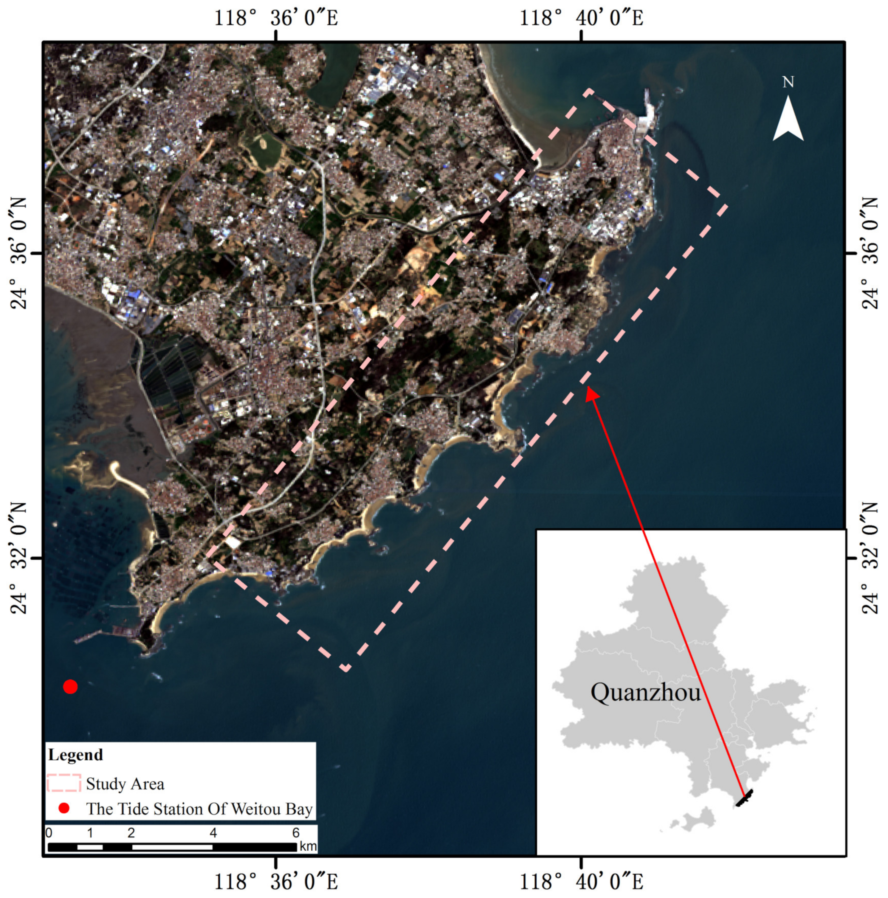
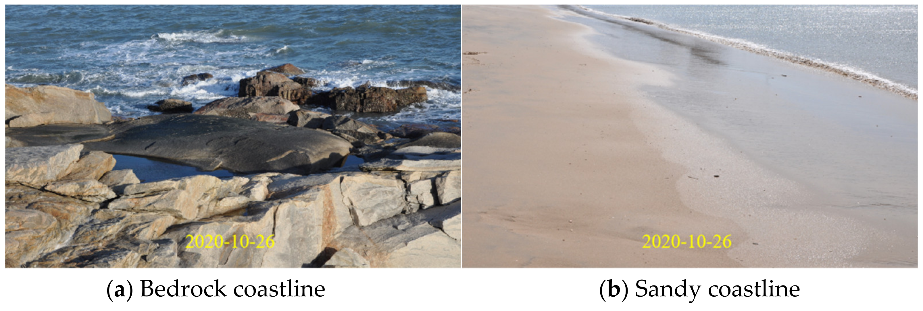
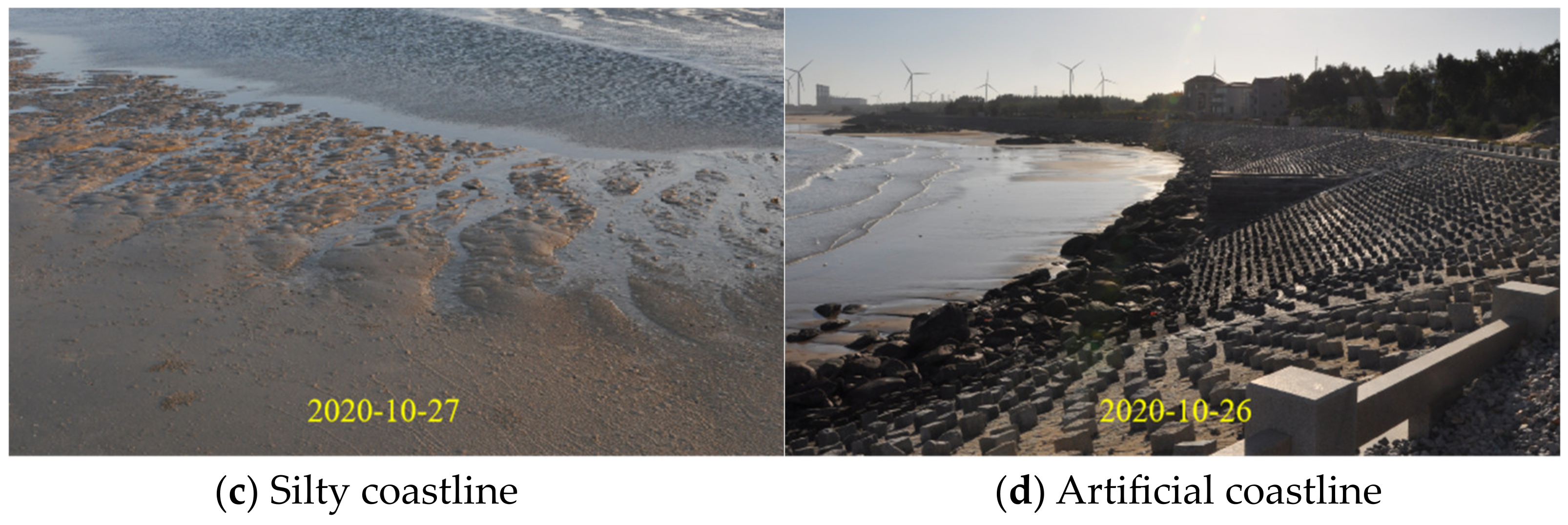
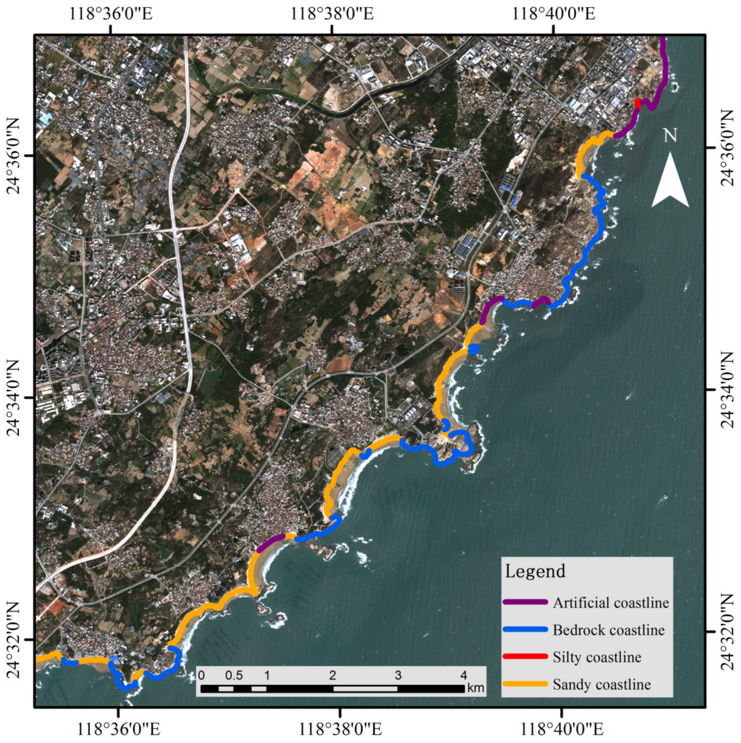
Weitou Bay is selected as our study area (Figure 1). The area is located in southeastern Quanzhou City, a famous coastal city of Fujian Province in China [38]. The study area falls under a subtropical monsoon climate, close to the Taiwan Strait, where the tidal range has a large spatial variation, with a mean tidal range of approximately 4 m [39]. In addition, the semi-diurnal tide is dominant in the Weitou Bay area [40], and the tidal state at the time of image acquisition is shown in Table 1. The coastline in this region can be categorized into two types: the natural coastline, unaffected by human development, and the artificial coastline, which is affected by human activities [41,42]. The natural coastlines in the study area include bedrock coastlines, sandy coastlines, and silty coastlines [43], while the coastlines dominated by artificial dikes are taken as artificial coastlines [44]. The coastline types are shown in Figure 2.
Quanzhou not only has a glorious history of two thousand years and is claimed to be one of the greatest ports in the world [45] but with the establishment of the national Belt and Road strategy, it has become the birthplace of the 21st century Maritime Silk Road, and its construction will have a great impact on the change exhibited by coastlines [46]. Quanzhou’s “Maritime Silk Road” was built into a characteristic cultural tourism product [47], and most religious sites are located along the coast [48]. In addition, part of the natural coastline was turned into an aquaculture shoreline through reclamation, which has changed the curvature and length of the shoreline [49]. These construction plans and activities are the main reasons for the observed coastline changes.
2.2. Satellite Image Download
A total of 21 Landsat-5 Thematic Mapper (TM) images, Landsat-7 Enhanced Thematic Mapper Plus (ETM+), and Landsat-8 Operational Land Imager (OLI) images covering the period from 2010 to 2020 were acquired from the USGS archives (https://www.usgs.gov/programs/usgs-library/collections) accessed on 21 October 2021. due to their low cloud coverage levels, as shown in Table 1. In addition, the datum, projection, resolution, path/row, and file type of each image are WGS84, UTM Zone 50 N, 30 × 30 m, 119/43, and TIFF, respectively. Two images, encompassing one from the first quarter and another from the third quarter, are selected annually. Moreover, the Landsat time-series images for the first and third quarters are separated by an approximate interval of six months. This temporal spacing is aligned with the typical capability of satellite-derived coastlines to effectively resolve the observed coastline variance in coastal features occurring over a time scale of six months or longer [50]. The images are in the L1TP format (radiometrically, geometrically, and topographically corrected) with reliable location accuracy. The first 20 scenes are used for model training, while the last scene is used for testing and accuracy evaluation purposes.
2.3. Data Preprocessing
As all Landsat images are from the USGS archive in the L1TP format with reliable location accuracy to support time-series analyses, image registration is not conducted. However, simulations have shown that atmospheric conditions, including water vapor concentrations and changes in optical thickness due to aerosols, play important roles and can result in digital number (DN) values [51]. Therefore, after using radiometric calibration to convert the DN values to radiances to compensate for atmospheric effects, fast line-of-sight atmospheric analysis of spectral hypercubes (FLAASH), a MODTRAN4-based atmospheric correction algorithm provided by ENVI software [52,53], is performed on all Landsat images.
To reduce the effects of clouds, including thin cirrus clouds and the thin edges of clouds, as well as their shadows, the Fmask algorithm (version 3.2), which was developed for cloud, cloud shadow, and snow detection in Landsat 4–7, 8, and Sentinel-2 images, is applied to each individual image [54,55].
To remove the effects of water bodies and improve the efficiency of the calculation process, the water bodies are extracted and masked off in each image using the modified normalized difference water index (MNDWI) according to the following equation [56]:
where is the reflection of a green channel such as TM band 2 or OLI band 3; is the reflection of a middle-infrared channel such as TM band 5 or OLI band 6, and MNDWI is the resulting MNDWI value.
3. Method
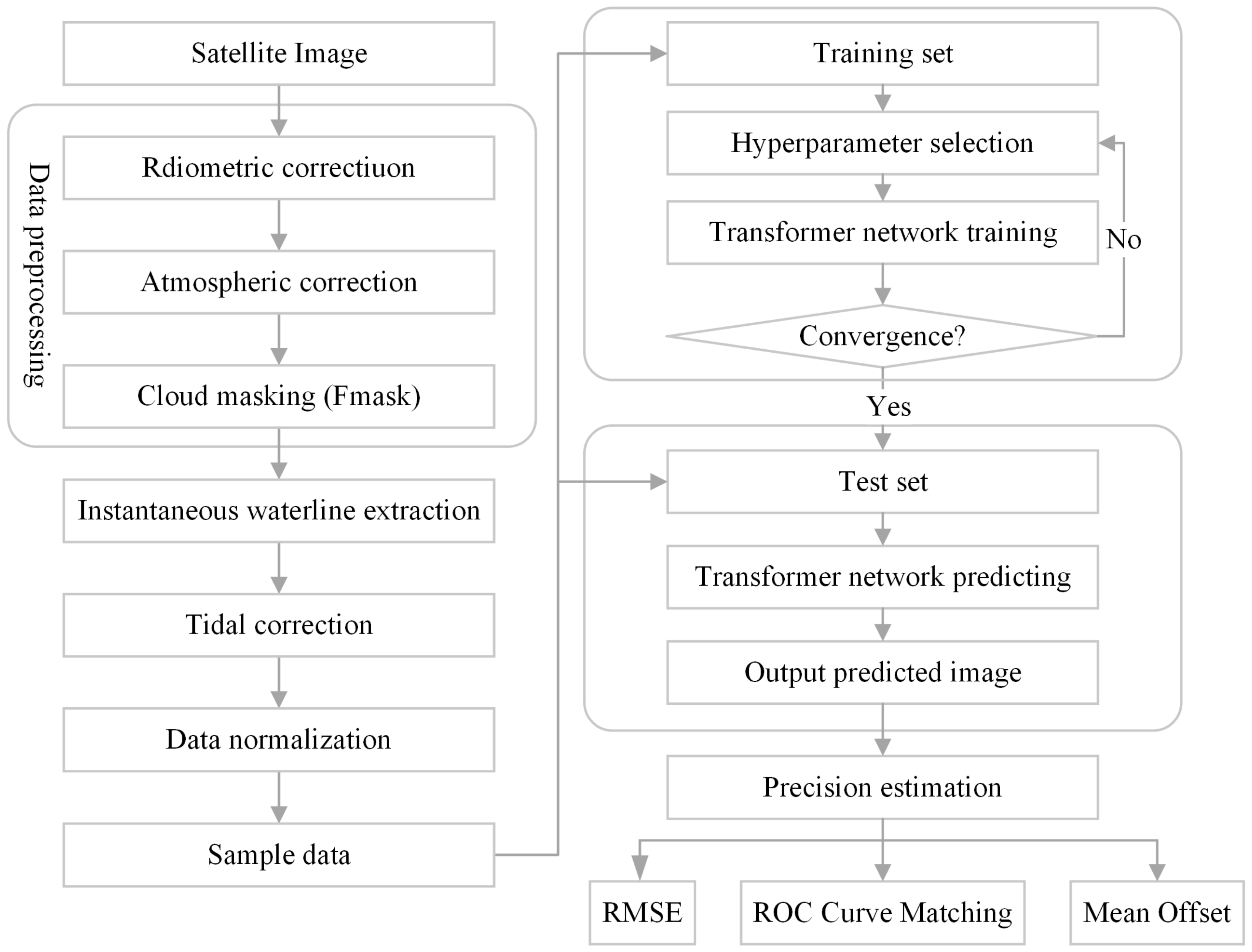
The study workflow is shown in Figure 3. After performing image preprocessing, the instantaneous waterline in each remotely sensed image is extracted using an active contour model [57]. As tide-level data are also important factors for predicting wave-dominated coastal areas [58], the tide-level data from the Weitou tidal station are then applied to adjust the instantaneous waterline to a coastline. This method is called tide correction. After completing data normalization, the acquired sample data are split into a training set and a test set. The training set serves the purpose of training the transformer model and fine-tuning the parameters to attain the optimal hyperparameters. Subsequently, the trained model is employed to predict outcomes using the test set as its input. Finally, the accuracy of the prediction results is assessed by comparing them with the accurate reference coastlines using three evaluation methods: the root mean square error (RMSE), receiver operating characteristic (ROC) curve-matching principle, and mean offset.
3.1. Instantaneous Waterline Extraction
In our study, the distance regularization level set evolution (DRLSE) model [59] is used to extract the instantaneous waterline via an energy functional formula:
where p(·) is the double-well potential function, δ(·) is the Dirac delta function, and H(·) is the Heaviside function. Additionally, g is the edge indicator function, and μ, λ > 0, and represent the constant coefficients of each energy term. The expression of the double-well potential function p(·) is defined as follows:
The edge indicator function g is defined as follows:
where is the Gaussian kernel of the parameter δ, and I is the image function.
In Equation (2), the first term of the energy functional represents the penalty energy term, which is commonly referred to as the distance regularization term. The inclusion of the distance regularization term effectively mitigates the irregular motion of the active contour during the evolution process, eliminating the need for repeated initialization and significantly enhancing the efficiency of image segmentation. The numerical solution of this model is based on the finite difference method, and the time step Δt must satisfy the convergence condition of the Courant–Friedrichs–Lewy (CFL) approach [60]. Toure et al. employed the DRLSE model to extract coastlines with specific experimental parameters [61], including μ = 0.2, λ = 5, α = 3, and Δt = 1. In this study, we adopt identical parameter settings in the experiments to maintain consistency. Initially, the DRLSE model is employed to obtain the instantaneous waterline, which is gradually derived from the initially defined active rectangular outline when approaching the feature boundary. At this stage, the extracted instantaneous waterline effectively demarcates the boundary of the land and water area, but some subtle deviations remain. Subsequently, the acquired edge contour undergoes refinement through manual visual interpretation, resulting in a more refined instantaneous waterline.
3.2. Tidal Correction
The extracted remote sensing image is the instantaneous waterline, which is intensively affected by the tide and must be considered in long-term coastline predictions. The tidal correction is based on the relationship between beach topography and tidal level changes, using the tidal height, tidal datum, and beach slope at the time of satellite imaging to calculate the horizontal distance from the instantaneous water boundary to the high tide line, so as to infer the location of the coastline. The tidal correction method assumes a constant slope across the coastline correction range, and the horizontal shift between instantaneous waterlines [50] is computed by the following formula:
where Δx is the cross-shore horizontal shift, zref is the reference tidal datum, ztide is the tidal elevation at the satellite image acquisition time, and m is a characteristic beach-face slope. The reference tidal datum and the tidal elevation are collected from the China National Seamen Service website (https://www.cnss.com.cn/tide/) accessed on 21 November 2021. The tidal datum at Weitou Bay is 322 cm below mean sea level. In this paper, the tidal-level data of the Tide Station of Weitou Bay located in the study area from 2010 to 2020 are collected in Table 1. m is calculated from two instantaneous waterlines extracted at different times:
where z1 and z2 are the tidal elevations at the times when the satellite images are acquired, and d is the average distance between the two extracted instantaneous waterlines.
3.3. Transformer Model
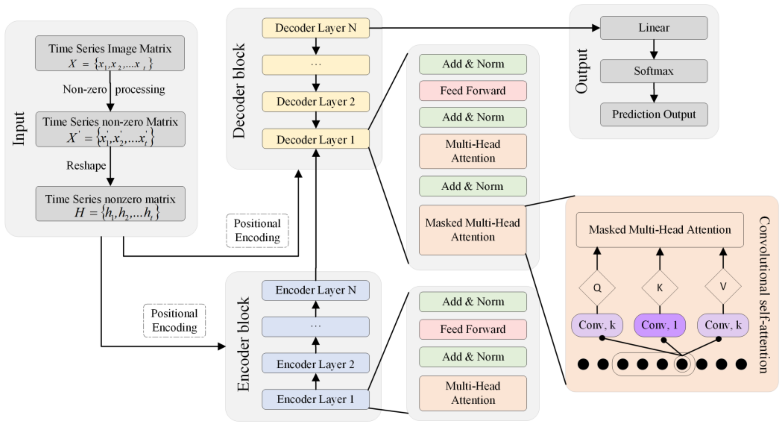
The overall architecture of the transformer model is depicted in Figure 4. The transformer model mainly consists of input, encoder block, decoder block, and output components, among which the encoder and decoder blocks are two critical parts [62].
First, we denote the time-series images as , where each corresponds to an image matrix at the ith time stamp. Here, t represents the total number of time-series images, while h and w represent the numbers of rows and columns in each image, respectively. Specifically, the pixel values in the training images are only 0 and 255 in the coastline prediction application investigated in this study, where 0 represents the background (non-coastline area) and 255 signifies a coastline. Second, considering the self-correlation of the multihead self-attention layer in the obtained transformer model, we define the 0 values in the image matrix as infinitesimal nonzero values so that the self-correlation attention layers are effective and meaningful when the dot product operations are executed. The processed nonzero time-series image matrix is denoted as . Third, we reshape each image matrix into a one-dimensional vector , where . n denotes the number of pixels in each image matrix, which equals . Fourth, the time-series sequence is divided into training samples and prediction samples, which undergo positional encoding and are fed into the encoder blocks and decoder blocks, respectively.
The encoder block includes a collection of encoders and is typically set to six layers [32]. Each encoder consists of a multihead self-attention sublayer and a fully connected feedforward sublayer. The multihead self-attention sublayer obtains the attention weight by calculating the similarity between the query and the key, which is essentially a variant of the input data. Then, the attention value can be computed as the weighted sum of their dot product. The fully connected feedforward sublayer contains two linear transformations and a rectified linear unit (ReLU) activation function. Residual concatenation is employed surrounding each sublayer, followed by data normalization. The output of the final encoder block is a continuous time-series sequence, which accounts for the self-correlation characteristics of the input sequence. The encoded data serve as an interactive input for the subsequent decoder blocks, facilitating the model in generating the predicted results.
Similarly, the decoder block also includes six decoders. In contrast to each encoder layer, each decoder incorporates an additional sublayer, enabling the interactive learning of multiple self-attention operations with the output of the encoder. In addition, the multihead self-attention mechanism of the encoder employs a mask to prevent the time-series data prediction process from learning future information. Finally, the decoder output is subjected to a linear transformation layer and a softmax layer, and the prediction results are derived by processing the matrix transformation by referring to the reverse process of the input layer.
Furthermore, the similarities between the queries and keys are calculated based on their pointwise values in the masked multihead attention layer of the canonical transformer, which results in abnormal observations if the local context is not fully utilized. Therefore, convolutional self-attention is used to mitigate this problem [63]. This model can better understand the local context by converting inputs into queries and keys using a causal convolution with a kernel size of k, a stride of size 1. Calculating their similarity through their local context information is helpful for obtaining accurate predictions.
3.4. Implementation Details
3.4.1. Redefined Image Format
To binarize the extracted coastline image for coastline extraction purposes, we assign a value of 255 to coastline pixels and a value of 0 to non-coastline pixels. A total of 20 images acquired from 2010 to 2019 are read to obtain an image pixel value matrix. Each pixel value matrix is mapped to a vector with 124,956 rows and 1 column, and a matrix with 124,956 rows and 20 columns is obtained after the combination operation. After determining the relative optimal hyperparameters, such as the time-step size, number of epochs, and causal convolutions with a kernel size of k, a matrix with 124,956 rows and 20 columns is input into the transformer model for training. The trained network is used to predict and output a vector with 124,956 rows and 1 column based on the coastline images of the previous years. Then, the pixel value matrix of the coastline image in the first quarter of 2020 is obtained through inverse mapping. Finally, the coastline prediction image for that year is output.
3.4.2. Training Strategies of SVR, LSTM, and Transformer Methods
In this paper, the transformer model is compared with a machine learning method SVR and a deep learning method LSTM, which have been proven to be robust coastline prediction methods [31,64].
Specifically, we employ the coastline position images extracted from Landsat time-series images from 2010 to 2019 as the training data for the three methods and the image from the first quarter of 2020 as the test data. The image of the coastline location in the first quarter of 2010 is denoted , where represents the first quarter. In practice, we trained the model to predict 1 future coastline image from 10 coastline data images of 5 years in one typical training setup. That is, the input of the model consisted of coastline position images from the first quarter of year 2010 to the third quarter of 2014, i.e., (, , , … ), and the output of the model aimed to obtain coastline results (, , , … ). Finally, the data are used to output the predicted coastlines , which is regarded as the test process, and the precision indexes of the predicted result are evaluated with the real coastline.
We conduct the SVR algorithm and perform hyperparameter optimization by the utilization of the sklearn and skopt packages in Python. Moreover, the LSTM model is configured with three hidden layers and an output layer. The LSTM model and the transformer model are implemented in the PyTorch toolbox with an NVIDIA GeForce RTX 2080 Ti GPU. The experiment is independently developed and realized based on the Pycharm platform and Python on a Windows 10 system.
3.5. Precision Validation
To evaluate the accuracy of the predicted coastline, this paper mainly adopts three evaluation indices to evaluate the results, including the ROC curve-matching principle, mean offset, and RMSE. Three indices are used to verify the accuracy between the real coastline (IWE + TC) and predicted coastline images.
3.5.1. ROC Curve-Matching Principle
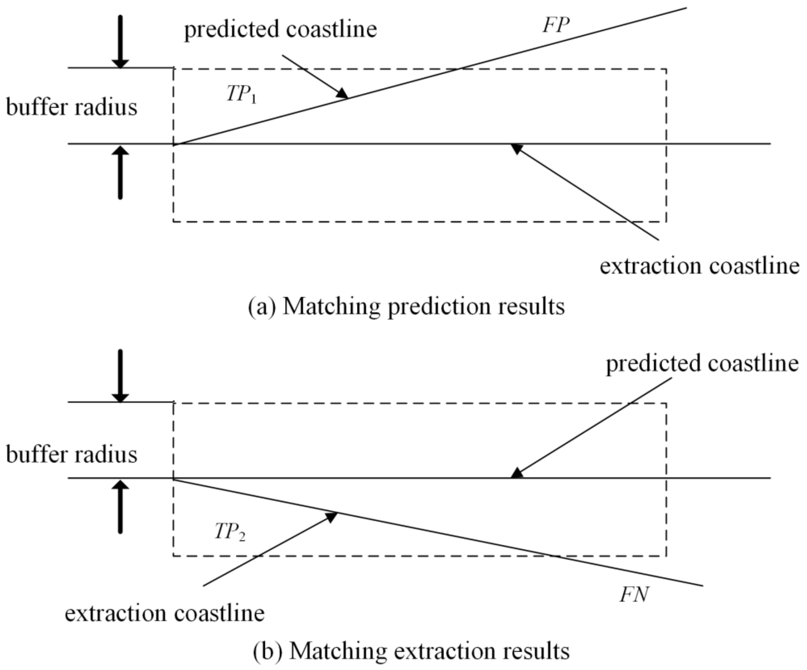
The ROC curve-matching principle, based on the spatial relationships along the coastline and not only considering the characteristics of the coastline but also matching a linear target to evaluate the accuracy of the coastline, is proposed [65]. This method first defines the accurately extracted coastline as a real coastline and then establishes a buffer zone with a buffer radius of n pixel units based on the real coastline. Thus, the real coastline and the predicted coastline are superimposed and analyzed. As shown in Figure 5, the true-positive (TP1) represents the length of the predicted coastline that was successfully matched within the established buffer, and the false-positive (FP) represents the length of the coastline that was not successfully matched. Similarly, a pixel-based buffer is built around the predicted coastline and subsequent coverage analysis is performed. In this case, TP2 represents the actual coastline length that was successfully matched in the buffer, while the false-negative (FN) represents the unmatched coastline length in the buffer.
Finally, the following parameters are used to evaluate the model accuracy:
where Complete represents the integrity of the coastline extraction results, Correct represents the accuracy of the coastline extraction results, and Quality is used to evaluate the extraction quality of the obtained coastline through the integration of correctness and integrity.
The coastline obtained by instantaneous waterline extraction and tidal correction (IWE + TC) is used as the accurate reference coastline, and the coastline predicted by the transformer model is used as the coastline to be tested. The number of pixels that fall into the buffer zone and the number of pixels that do not fall into the buffer zone are used to replace the coastline length for the accuracy verification.
3.5.2. Mean Offset and Root Mean Square Error
The mean offset and RMSE are commonly used in coastline accuracy verifications [66]:
where n is the total number of sample points, and D is the Euclidean distance from the coastline feature points in the reference coastline dataset to the extracted coastline.
We calculate the Euclidean distances from the predicted coastline pixels to the accurate coastline pixels. Pixels with distances of less than one pixel are classified as successfully predicted pixels; conversely, pixels with distances larger than one pixel are classified as failed pixels. The ROC matching principle is adopted to establish a buffer area based on coastline extraction. The coastline obtained by IWE + TC is used as the accurate coastline, and the coastlines predicted by the three methods are used as the coastlines to be evaluated.
According to the coastline images extracted and predicted in the first quarter of 2020, the accuracy of the prediction results is evaluated by the ROC curve-matching principle, mean offset, and RMSE, and an accuracy analysis is carried out in combination with the coastline type and tidal correction.
4. Results
4.1. Coastline Extraction
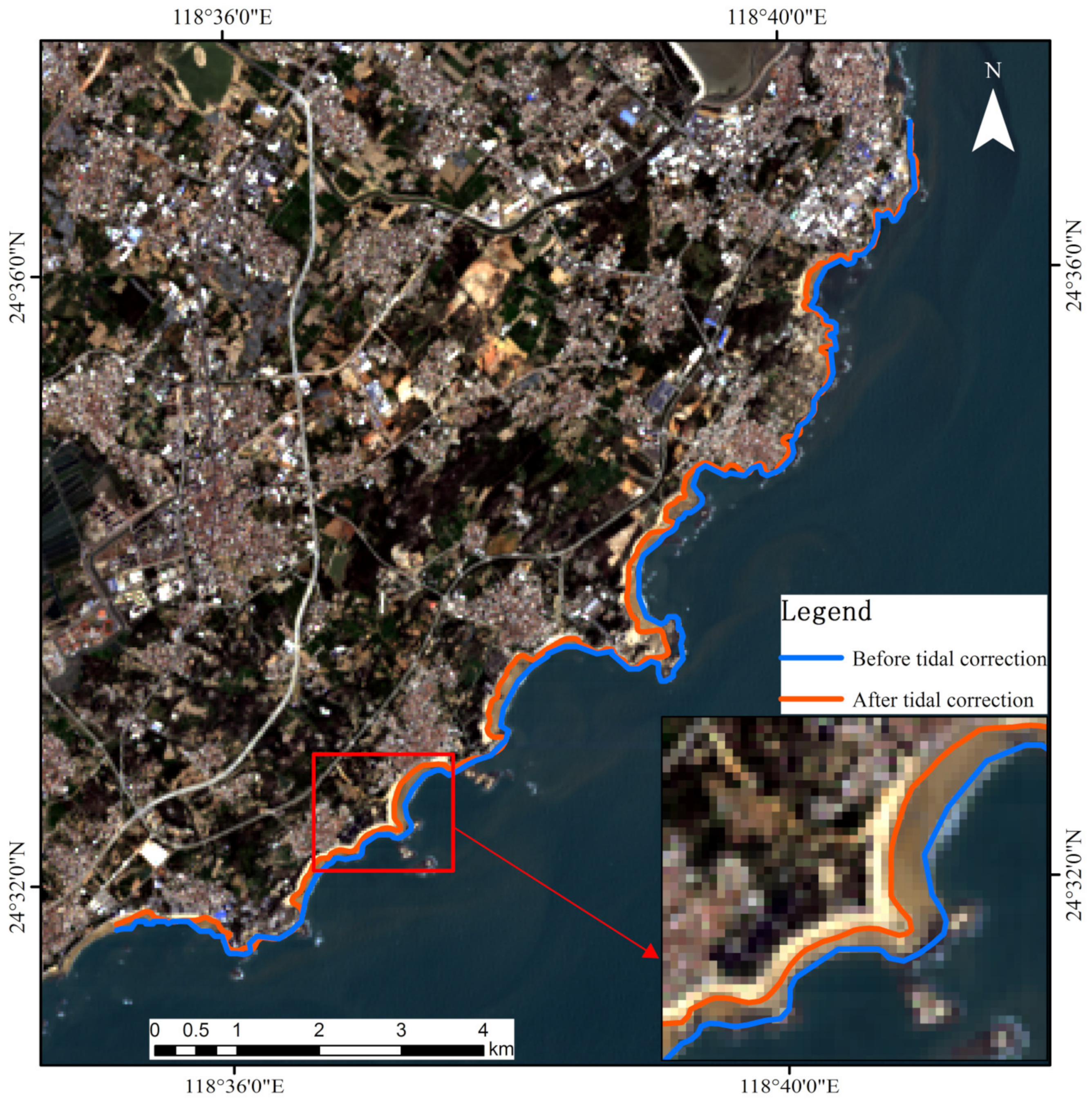
Figure 6 illustrates the instantaneous waterlines obtained by executing the DRLSE model and manual correction on the given remote sensing image, followed by the derivation of the coastline through tide correction. The accuracy of the coastline obtained by the IWE + TC method is verified through a visual inspection. The instantaneous waterline is represented in blue, while the coastline, corrected for tidal influences, is denoted by the orange curve. Additionally, a partial enlargement is provided in the lower-right corner.
4.2. Predicted Coastline
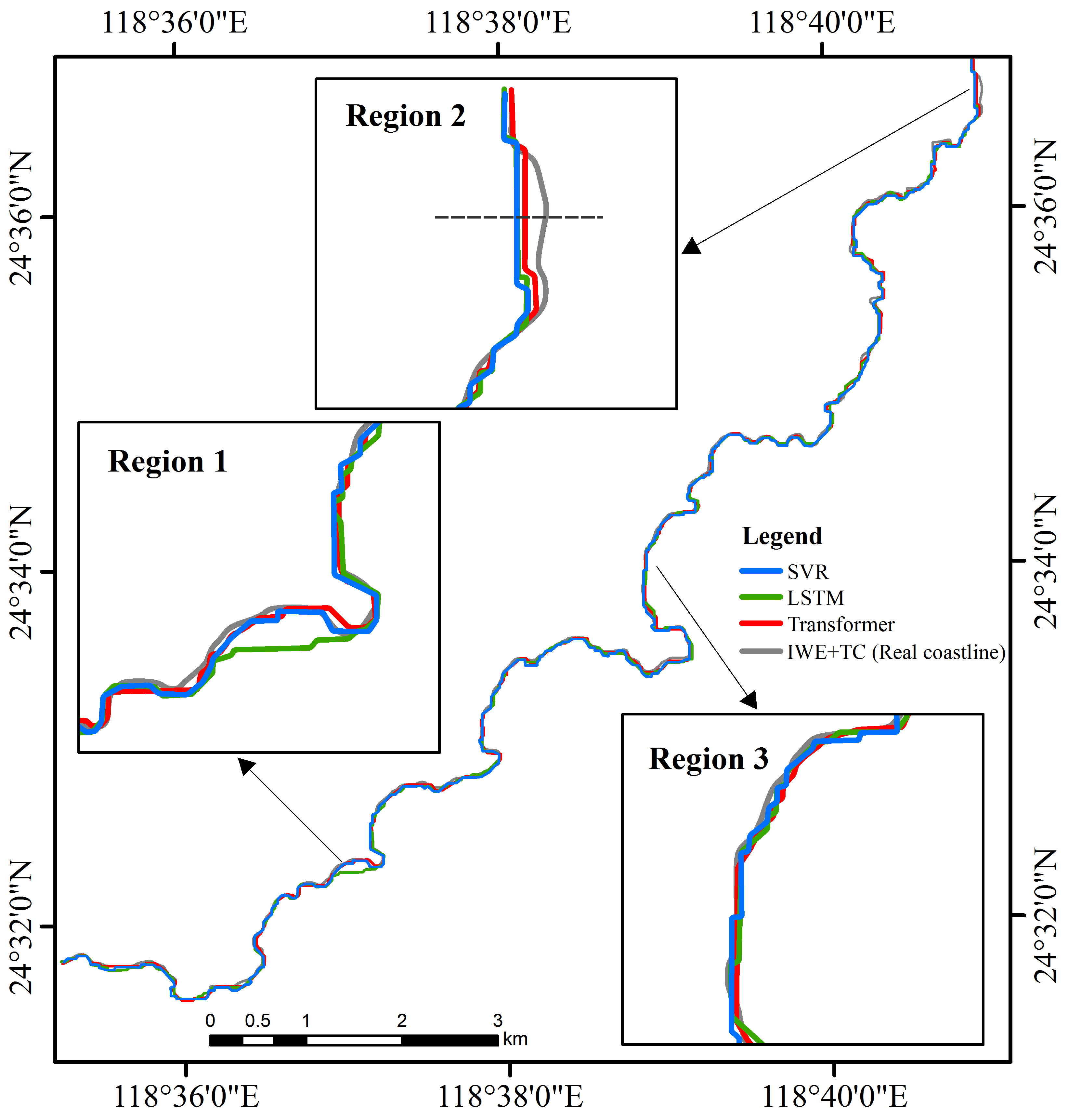
Figure 7 depicts the predicted results obtained for the transformer, SVR, and LSTM coastlines in the first quarter of 2020. Each predicted coastline image is compared with the real coastline, and the overlapping areas are the parts with good prediction effects. In contrast, the prediction results contain errors.
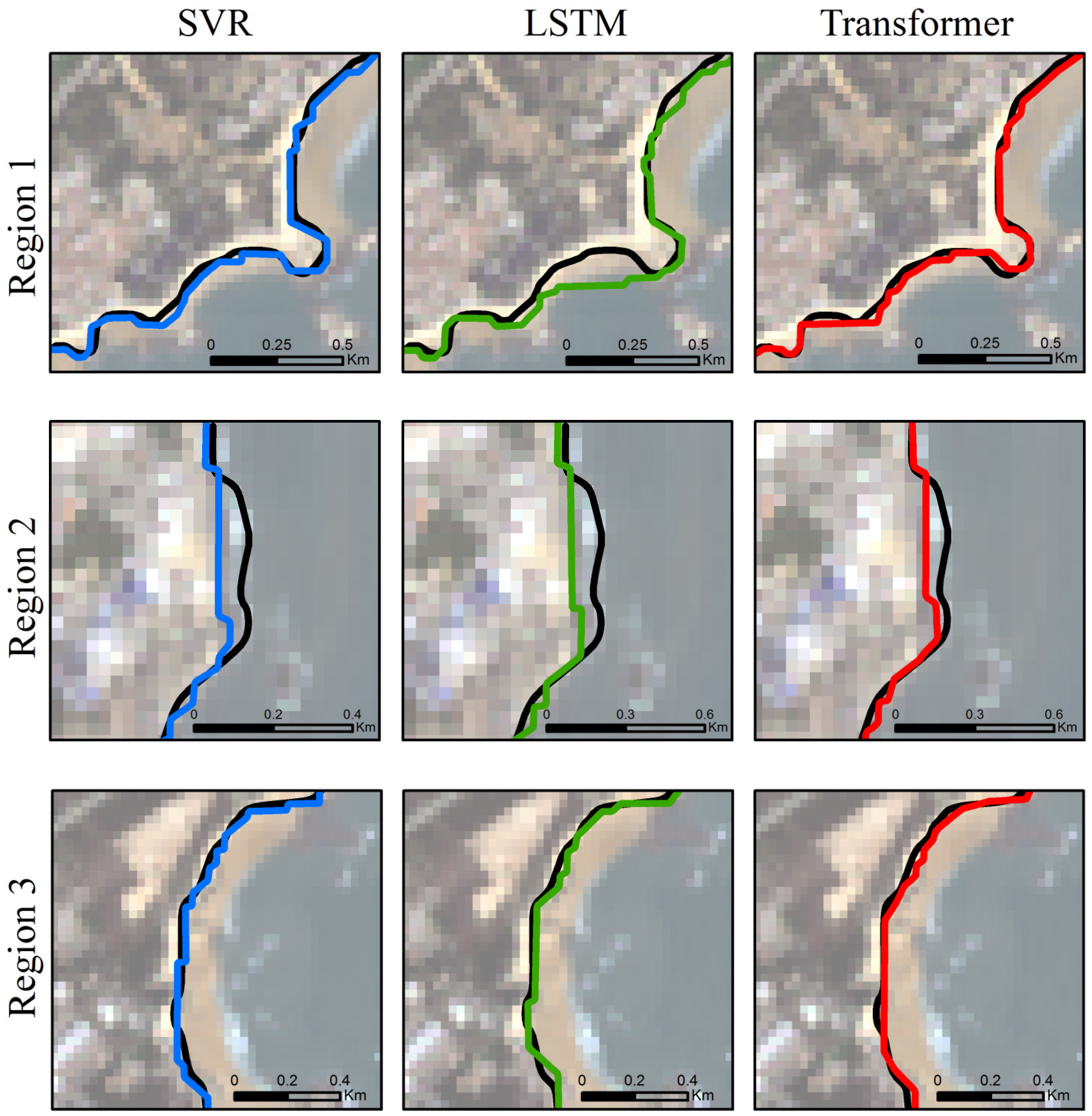
In addition, to further analyze the details of the predicted coastline results, three typical regions are selected in Figure 7, and their overlaps with the accurate coastline are shown in Figure 8. The coastline predicted by the LSTM model in Region 1 does not coincide with the real coastline according to the overlap comparison between the coastline results predicted by the three models and the real coastline, while the results of the transformer model and SVR model basically coincide with the real coastline. Region 2 indicates that the coastlines predicted by the three models are approximately located in the same position, and the coastline predicted by the transformer model is closest to the real coastline. Specifically, the distance of the prediction error is measured by vertical lines from the real coastline to the intersection of the predicted coastline of the three methods. We select the point where the disparity is most pronounced as a sample in Region 2 of Figure 7 (represented by a black dotted line), which reflects that the discrepancies between the coastlines predicted by the Transformer, LSTM, and SVR methods, compared to the real coastline, are 55.34 m, 77.48 m, and 78.01 m, respectively. These differences all exceed one pixel (30 m). In Region 3, the coastlines predicted by the three models all coincide well with the real coastline within one pixel, which indicates that these models have the ability and potential to predict future coastlines.
4.3. Accuracy Evaluation
Table 2 shows the accuracy of the results predicted by the three methods through the ROC curve-matching principle, mean offset, and RMSE metrics.
We individually analyzed the pixels that represent the coastlines in the resulting images obtained by prediction. For the Weitou Bay area, the correct, complete and quality values of the coastline predicted by the transformer model for the first quarter of 2020 are 98.80%, 96.40%, and 95.24%, respectively. All pixels of the predicted coastline are considered sample points, and the calculated mean offset and RMSE are 0.32 pixels and 0.57 pixels, respectively, as shown in Table 2.
SVR and LSTM are used for comparison with the transformer model. The precision evaluations of the coastlines predicted for the first quarter of 2020 by the SVR and LSTM models are shown in Table 2. The quality of the coastline predicted by SVR is 76.57%, which is 18.67% lower than that of the result predicted by the transformer model. The RMSE of the SVR method is 0.85 pixels, which is 0.28 pixels higher than that of the transformer. Similarly, the quality of the coastline predicted by the LSTM method is 9.15% lower than that predicted by the transformer method, and its RMSE is 0.22 pixels higher than that predicted by the transformer method.
5. Discussions
Our study has demonstrated that the predictions of the three models generally coincide with the real coastline extracted by the IWE + TC method in most areas of the Weitou Bay region, and the result of the transformer model exhibits the closest agreement with the real coastline in some challenging regions, which is better than the performance of the LSTM and SVR models.
In recent years, ecological security issues such as the lack of ecosystem services in the coastal zone of Weitou Bay area have attracted great attention due to rapid urbanization and industrialization [67]. These human activities also affect the changes in the coastline in the Weitou Bay area. Most of the research on coastline prediction has mainly relied on traditional techniques such as numerical models, physical models, and field measurement data analysis methods, while the use of deep learning methods remains relatively limited. As one of the state-of-the-art deep learning models, the transformer model gives more accurate prediction results concerning the change trend of the coastline in the Weitou Bay area, which can be further used in the environmental protection against beach loss [68,69], the maintenance of coastal disaster warning systems [70], as well as the management of coastal land [71,72].
Coastline dynamics are frequently affected by tidal correction and coastline type [73,74]. Tidal variation and the elevation of the tidal flat have great influence on the precision of coastline location estimation and the historical changes in coastline. Additionally, the type of coastline and the extent of land-use change are also intertwined with the accuracy of coastline prediction, which directly affects the coastline stability. The effects of these two factors on the prediction results are discussed in the following section.
5.1. The Effect of Tidal Correction
Tidal correction plays an important role in coastline prediction. To demonstrate the key role of tidal correction in coastline prediction, an ablation experiment is conducted. The experiment used coastal data, both before and after tidal correction, to perform predictions and evaluations of the transformer model to obtain the coastline for the coming year. The precision values are shown in Table 3, indicating the obvious improvements in results when tidal correction is applied.
5.2. Effects of Coastline Types on Prediction
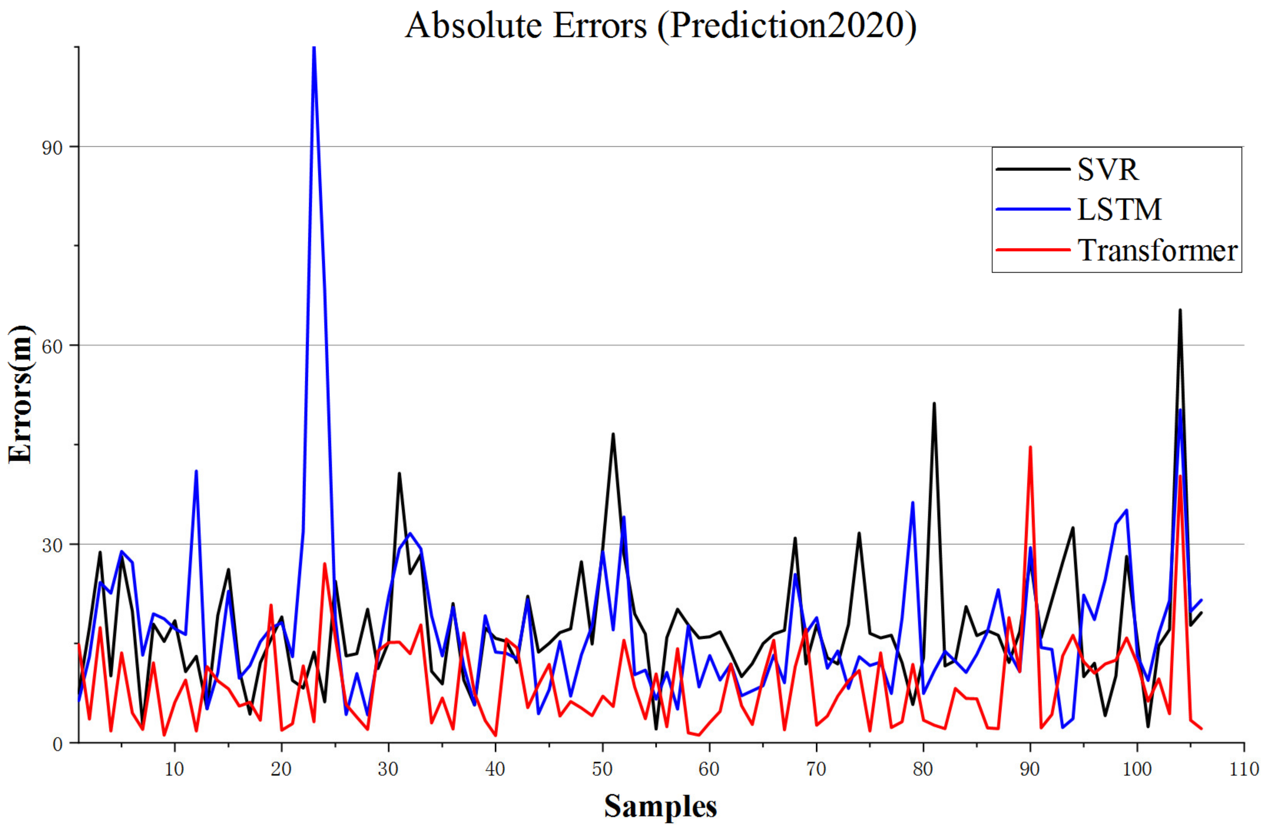
Figure 9 shows the deviation of the predicted coastline image for the first quarter of 2020 from the sample points of the exact coastline for the first quarter of 2020. The y-axis (m) denotes the absolute error, and the x-axis denotes the sample points. The coastline sample points are sampled at 200-m intervals, and the Euclidean distances from these sample points to the predicted coastline points are calculated. Figure 10 shows the distribution of coastline types in Weitou Bay in 2017 through Gaofen-2 images (the coastline types in the Weitou Bay area in 2020 were the same as those in 2017). In Figure 9, the coastline prediction results clearly reflect that the prediction results of the transformer model are better than those of the SVR model and LSTM model, and larger absolute errors are induced by the results obtained for the 24th sample and the 104th sample. The 24th sample point is located in a sandy coastline area, and the fluctuation of this coastline type is relatively stable. Because the image used in the experiment corresponds to 30 m per pixel, the errors of the prediction results yielded by the SVR and transformer methods can be equivalent to less than one pixel, and the error of the LSTM model is more than three pixels. Therefore, the LSTM method is insufficient for accurately predicting this area. The error value of the 104th sample point shows a sudden change when the coastline prediction results of the three prediction methods all exceed one pixel in this sample point. Specifically, we find that this sample point is located within the confines of a shipping company, which belongs to an artificial coastline area. In addition, Table 4 shows the RMSEs produced for the four coastline types obtained by the three prediction methods. The RMSE of artificial shorelines is larger than those of bedrock coastlines, sandy coastlines, and silt coastlines. In summary, artificial coastline areas are often subject to frequent human-made reconstructions and are greatly affected by human activities. Many anthropogenic interferences are predicted, and the results cannot be effectively obtained.
6. Conclusions
This paper collects Landsat-8, Landsat-7 and Landsat-5 satellite data from the Weitou Bay area of Quanzhou city, Fujian Province, from the first and third quarters of 2010 to 2020 biannually. After preprocessing the satellite images with ENVI, the instantaneous waterline of the first and third quarters each year is extracted. Moreover, the tide-level data acquired from the Weitou Bay tide station are used to correct the extracted coastline data to obtain the real coastline position data for the prediction reference. Finally, the pixel-by-pixel predictions of three models are used to deduce the coastline position for the Weitou Bay area in the first quarter of 2020. The transformer model used in this paper performs better prediction accuracy compared with the SVR and LSTM models. In an ROC curve accuracy verification, the complete, correct and quality values of the transformer method are 98.80%, 96.40%, and 95.24%, respectively, which are all above 90%, and the mean offset and RMSE are 0.32 pixels and 0.57 pixels. In addition, the necessity of tide correction is verified from the comparative ablation experiment. Furthermore, different prediction effects for different types of coastlines in the Weitou Bay area are discussed by transformer method. For natural coastlines, including sandy coastlines, silt coastlines, and bedrock coastlines, the coastline prediction results have high accuracy and strong continuity. For artificial coastlines, including dams, wharves, and reclamation areas, some of the prediction results are inferior due to the influence of human activities.
The results obtained are not only crucial for analyzing coastline changes in the Weitou Bay area but also can be further applied for broader applications in other coastal regions. The exploration of methods to predict the location of unknown coastlines is of great significance for environmental protection departments and land planning departments to manage land use and coastline development in coastal regions. However, there are still some limitations, including the challenges of (1) optimizing the transformer model to obtain optimal hyperparameters, necessitating the use of more efficient hyperparameter optimization methods; (2) ensuring the retention of spatial information during the process of mapping the image matrix to a vector; and (3) addressing issues related to data collection and quality, which are influenced by the limited satellite data and changes in coastal climate conditions.
In the future, the modelling and matrix transformation methods can be improved while preserving spatial information by using better hyperparameter optimization methods to obtain better hyperparameter combinations and achieve improved prediction efficiency. Simultaneously, we also intend to augment the generalization capability and robustness of the transformer model by incorporating an extended temporal range and broader geographical scope from additional remote sensing time-series data.
Author Contributions
Conceptualization, Z.Y. and G.W. (Guangjun Wang); methodology, Z.Y. and Y.W.; software, Z.Y. and Y.W.; validation, Z.Y.; formal analysis, Z.Y.; investigation, Z.Y. and G.W. (Guangjun Wang); resources, G.W. (Guangjun Wang) and S.L.; data curation, Z.Y. and G.W. (Guowei Wang); writing—original draft preparation, Z.Y.; writing—review and editing, G.W. (Guangjun Wang); visualization, Z.Y.; supervision, L.F.; project administration, G.W. (Guangjun Wang); funding acquisition, G.W. (Guangjun Wang). All authors have read and agreed to the published version of the manuscript.
Funding
This work was supported by the Geological Survey Project of China Geological Survey (DD20191006), and the Strategic Priority Research Program of the Chinese Academy of Sciences (XDA20100103).
Acknowledgments
We would like to thank the anonymous reviewers for their constructive input in the manuscript.
Conflicts of Interest
The authors declare no conflict of interest.
References
- Boak, E.H.; Turner, I.L. Shoreline definition and detection: A review. J. Coast. Res. 2005, 21, 688–703. [Google Scholar] [CrossRef]
- Cui, B.-L.; Li, X.-Y. Coastline change of the Yellow River estuary and its response to the sediment and runoff (1976–2005). Geomorphology 2011, 127, 32–40. [Google Scholar] [CrossRef]
- Genz, A.S.; Fletcher, C.H.; Dunn, R.A.; Frazer, L.N.; Rooney, J.J. The predictive accuracy of shoreline change rate methods and alongshore beach variation on Maui, Hawaii. J. Coast. Res. 2007, 23, 87–105. [Google Scholar] [CrossRef]
- Scott, D.B. Coastal changes, rapid. In Encyclopedia of Coastal Sciences; Springer: Cham, The Netherlands, 2005; pp. 253–255. [Google Scholar]
- Kumar, A.; Jayappa, K. Long and short-term shoreline changes along Mangalore coast, India. Int. J. Environ. Res. 2009, 3, 177–188. [Google Scholar] [CrossRef]
- Larson, M.; Kraus, N.C. Prediction of cross-shore sediment transport at different spatial and temporal scales. Mar. Geol. 1995, 126, 111–127. [Google Scholar] [CrossRef]
- Miller, J.K.; Dean, R.G. A simple new shoreline change model. Coast. Eng. 2004, 51, 531–556. [Google Scholar] [CrossRef]
- Li, Z.; Chen, Z. Progress in the Studies on Shoreline Change of Sandy Coast. Mar. Sci. Bull. 2003, 22, 77–86. [Google Scholar]
- Chen, X.; Zong, Y. Coastal erosion along the Changjiang deltaic shoreline, China: History and prospective. Estuar. Coast. Shelf Sci. 1998, 46, 733–742. [Google Scholar] [CrossRef]
- Davidson, M.A.; Lewis, R.P.; Turner, I.L. Forecasting seasonal to multi-year shoreline change. Coast. Eng. 2010, 57, 620–629. [Google Scholar] [CrossRef]
- Hughes, S.A. Physical Models and Laboratory Techniques in Coastal Engineering; World Scientific: Singapore, 1993. [Google Scholar]
- Ekphisutsuntorn, P.; Wongwises, P.; Chinnarasri, C.; Humphries, U.; Vongvisessomjai, S. Numerical modeling of erosion for muddy coast at Bangkhuntien shoreline, Thailand. Int. J. Environ. Sci. Eng. 2010, 2, 230–240. [Google Scholar]
- Nguyen, X.T.; Tran, M.T.; Tanaka, H.; Nguyen, T.V.; Mitobe, Y.; Duong, C.D. Numerical investigation of the effect of seasonal variations of depth-of-closure on shoreline evolution. Int. J. Sediment Res. 2021, 36, 1–16. [Google Scholar] [CrossRef]
- Thanh, T.M.; Tanaka, H.; Mitobe, Y.; Viet, N.T.; Almar, R. Seasonal variation of morphology and sediment movement on nha trang coast, vietnam. J. Coast. Res. 2018, 81, 22–31. [Google Scholar]
- Zeinali, S.; Dehghani, M.; Talebbeydokhti, N. Artificial neural network for the prediction of shoreline changes in Narrabeen, Australia. Appl. Ocean. Res. 2021, 107, 102362. [Google Scholar] [CrossRef]
- Adamo, F.; De Capua, C.; Filianoti, P.; Lanzolla, A.M.L.; Morello, R. A coastal erosion model to predict shoreline changes. Measurement 2014, 47, 734–740. [Google Scholar] [CrossRef]
- Douglas, B.C.; Crowell, M. Long-term shoreline position prediction and error propagation. J. Coast. Res. 2000, 16, 145–152. [Google Scholar]
- Ghorai, D.; Bhunia, G.S. Automatic shoreline detection and its forecast: A case study on Dr. Abdul Kalam Island in the section of Bay of Bengal. Geocarto Int. 2022, 37, 2273–2292. [Google Scholar] [CrossRef]
- Ciritci, D.; Türk, T. Assessment of the Kalman filter-based future shoreline prediction method. Int. J. Environ. Sci. Technol. 2020, 8, 3801–3816. [Google Scholar] [CrossRef]
- San, B.T.; Ulusar, U.D. An approach for prediction of shoreline with spatial uncertainty mapping (SLiP-SUM). Int. J. Appl. Earth Obs. Geoinf. 2018, 73, 546–554. [Google Scholar] [CrossRef]
- Addo, K.A.; Walkden, M.; Mills, J.T. Detection, measurement and prediction of shoreline recession in Accra, Ghana. ISPRS J. Photogramm. Remote Sens. 2008, 63, 543–558. [Google Scholar] [CrossRef]
- Carleo, G.; Cirac, I.; Cranmer, K.; Daudet, L.; Schuld, M.; Tishby, N.; Vogt-Maranto, L.; Zdeborová, L. Machine learning and the physical sciences. Rev. Mod. Phys. 2019, 91, 045002. [Google Scholar] [CrossRef]
- Cortes, C.; Vapnik, V. Support-vector networks. Mach. Learn. 1995, 20, 273–297. [Google Scholar] [CrossRef]
- Tuia, D.; Verrelst, J.; Alonso, L.; Pérez-Cruz, F.; Camps-Valls, G. Multioutput support vector regression for remote sensing biophysical parameter estimation. IEEE Geosci. Remote Sens. Lett. 2011, 8, 804–808. [Google Scholar] [CrossRef]
- Parbat, D.; Chakraborty, M. A python based support vector regression model for prediction of COVID19 cases in India. Chaos Solitons Fractals 2020, 138, 109942. [Google Scholar] [CrossRef] [PubMed]
- Balabin, R.M.; Lomakina, E.I. Support vector machine regression (SVR/LS-SVM)—An alternative to neural networks (ANN) for analytical chemistry? Comparison of nonlinear methods on near infrared (NIR) spectroscopy data. Analyst 2011, 136, 1703–1712. [Google Scholar] [CrossRef] [PubMed]
- Ramedani, Z.; Omid, M.; Keyhani, A.; Khoshnevisan, B.; Saboohi, H. A comparative study between fuzzy linear regression and support vector regression for global solar radiation prediction in Iran. Sol. Energy 2014, 109, 135–143. [Google Scholar] [CrossRef]
- Goncalves, R.M.; Awange, J.L.; Krueger, C.P.; Heck, B.; Dos Santos Coelho, L. A comparison between three short-term shoreline prediction models. Ocean Coast. Manag. 2012, 69, 102–110. [Google Scholar] [CrossRef]
- Chang, F.-J.; Lai, H.-C. Adaptive neuro-fuzzy inference system for the prediction of monthly shoreline changes in northeastern Taiwan. Ocean Eng. 2014, 84, 145–156. [Google Scholar] [CrossRef]
- Pazou, M.G.A.; Agbodoyetin, A.; Akowanou, C. Shoreline evolution prediction using satellite images and time series analysis techniques: Case of Akpakpa shoreline in Benin Republic. In Proceedings of the 2022 International Conference on Electrical, Computer, Communications and Mechatronics Engineering (ICECCME), Maldives, 16–18 November 2022; IEEE: New York, NY, USA, 2022. [Google Scholar]
- Yin, C.; Anh, D.T.; Mai, S.T.; Le, A.; Nguyen, V.-H.; Nguyen, V.-C.; Tinh, N.X.; Tanaka, H.; Viet, N.T.; Nguyen, L.D. Advanced machine learning techniques for predicting nha trang shorelines. IEEE Access 2021, 9, 98132–98149. [Google Scholar] [CrossRef]
- Vaswani, A.; Shazeer, N.; Parmar, N.; Uszkoreit, J.; Jones, L.; Gomez, A.N.; Kaiser, Ł.; Polosukhin, I. Attention is all you need. Adv. Neural Inf. Process. Syst. 2017, 30, 6000–6010. [Google Scholar]
- Mohammadi Farsani, R.; Pazouki, E. A transformer self-attention model for time series forecasting. J. Electr. Comput. Eng. Innov. JECEI 2020, 9, 1–10. [Google Scholar]
- Wu, N.; Green, B.; Ben, X.; O’banion, S. Deep transformer models for time series forecasting: The influenza prevalence case. arXiv 2020, arXiv:200108317. [Google Scholar]
- Cai, L.; Janowicz, K.; Mai, G.; Yan, B.; Zhu, R. Traffic transformer: Capturing the continuity and periodicity of time series for traffic forecasting. Trans. GIS 2020, 24, 736–755. [Google Scholar] [CrossRef]
- Zhang, C.; Wang, L.; Cheng, S.; Li, Y. SwinSUNet: Pure transformer network for remote sensing image change detection. IEEE Trans. Geosci. Remote Sens. 2022, 60, 1–13. [Google Scholar] [CrossRef]
- Chen, H.; Qi, Z.; Shi, Z. Remote sensing image change detection with transformers. IEEE Trans. Geosci. Remote Sens. 2021, 60, 1–14. [Google Scholar] [CrossRef]
- Yang, D.; Qi, S.; Zhang, Y.; Xing, X.; Liu, H.; Qu, C.; Liu, J.; Li, F. Levels, sources and potential risks of polycyclic aromatic hydrocarbons (PAHs) in multimedia environment along the Jinjiang River mainstream to Quanzhou Bay, China. Mar. Pollut. Bull. 2013, 76, 298–306. [Google Scholar] [CrossRef] [PubMed]
- Zhang, W.Z.; Shi, F.; Hong, H.S.; Shang, S.P.; Kirby, J.T. Tide-surge interaction intensified by the Taiwan Strait. J. Geophys. Res. Ocean. 2010, 115. [Google Scholar] [CrossRef]
- Zhu, J.; Hu, J.; Zhang, W.; Zeng, G.; Chen, D.; Chen, J.; Shang, S. Numerical study on tides in the Taiwan Strait and its adjacent areas. Mar. Sci. Bull. 2009, 11, 23–36. [Google Scholar]
- Wu, T.; Hou, X.; Xu, X. Spatio-temporal characteristics of the mainland coastline utilization degree over the last 70 years in China. Ocean Coast. Manag. 2014, 98, 150–157. [Google Scholar] [CrossRef]
- Sun, X.; Zhang, L.; Lu, S.-Y.; Tan, X.-Y.; Chen, K.-L.; Zhao, S.-Q.; Huang, R.-H. A new model for evaluating sustainable utilization of coastline integrating economic output and ecological impact: A case study of coastal areas in Beibu Gulf, China. J. Clean. Prod. 2020, 271, 122423. [Google Scholar] [CrossRef]
- Gong, X.; Qi, S.; Wang, Y.; Julia, E.; Lv, C. Historical contamination and sources of organochlorine pesticides in sediment cores from Quanzhou Bay, Southeast China. Mar. Pollut. Bull. 2007, 54, 1434–1440. [Google Scholar] [CrossRef]
- Wu, Y.; Liu, Z. Research progress on methods of automatic coastline extraction based on remote sensing images. J. Remote Sens. 2019, 23, 582–602. [Google Scholar] [CrossRef]
- Li, R.; Wang, Q.; Cheong, K.C. Quanzhou: Reclaiming a glorious past. Cities 2016, 50, 168–179. [Google Scholar] [CrossRef]
- Gao, T.; Na, S.; Dang, X.; Zhang, Y. Study of the Competitiveness of Quanzhou Port on the Belt and Road in China Based on a Fuzzy-AHP and ELECTRE III Model. Sustainability 2018, 10, 1253. [Google Scholar] [CrossRef]
- Zheng, X. Countermeasures for development of Fujian cultural tourism based on SWOT analysis. In Proceedings of the 3rd International Conference on Culture, Education and Economic Development of Modern Society (ICCESE 2019), Moscow, Russia, 1 March 2019; Atlantis Press: Amsterdam, The Netherlands, 2019. [Google Scholar]
- Fan, L.; Cao, M.; Li, X. Analysis of the Temporal and Spatial Distribution Characteristics and Influencing Factors of Religious Sites on the Maritime Silk Road: A Case Study of Quanzhou. J. Tour. Manag. Res. 2022, 9, 110–124. [Google Scholar] [CrossRef]
- Xiao, X.; Li, Y.; Shu, F.; Wang, L.; He, J.; Zou, X.; Chi, W.; Lin, Y.; Zheng, B. Coupling relationship of human activity and geographical environment in stage-specific development of urban coastal zone: A case study of Quanzhou Bay, China (1954–2020). Front. Mar. Sci. 2022, 8, 781910. [Google Scholar] [CrossRef]
- Vos, K.; Harley, M.D.; Splinter, K.D.; Simmons, J.A.; Turner, I.L. Sub-annual to multi-decadal shoreline variability from publicly available satellite imagery. Coast. Eng. 2019, 150, 160–174. [Google Scholar] [CrossRef]
- Holben, B.N. Characteristics of maximum-value composite images from temporal AVHRR data. Int. J. Remote Sens. 1986, 7, 1417–1434. [Google Scholar] [CrossRef]
- Cooley, T.; Anderson, G.P.; Felde, G.W.; Hoke, M.L.; Ratkowski, A.J.; Chetwynd, J.H.; Gardner, J.A.; Adler-Golden, S.M.; Matthew, M.W.; Berk, A.; et al. FLAASH, a MODTRAN4-based atmospheric correction algorithm, its application and validation. In Proceedings of the IEEE International Geoscience and Remote Sensing Symposium 2003, Toronto, ON, Canada, 24–28 June 2002. [Google Scholar]
- Berk, A.; Anderson, G.P.; Bernstein, L.S.; Acharya, P.K.; Dothe, H.; Matthew, M.W.; Adler-Golden, S.M.; Chetwynd, J.H., Jr.; Richtsmeier, S.C.; Pukall, B.; et al. MODTRAN4 radiative transfer modeling for atmospheric correction. In Proceedings of the 1999 Optical Spectroscopic Techniques and Instrumentation for Atmospheric and Space Research III, Denver, CO, USA, 19–21 July 1999; Society of Photo-Optical Instrumentation Engineers: Washington, DC, USA, 1999. [Google Scholar]
- Zhu, Z.; Wang, S.; Woodcock, C.E. Improvement and expansion of the Fmask algorithm: Cloud, cloud shadow, and snow detection for Landsats 4-7, 8, and Sentinel 2 images. Remote Sens Environ. 2015, 159, 269–277. [Google Scholar] [CrossRef]
- Zhu, Z.; Woodcock, C.E. Object-based cloud and cloud shadow detection in Landsat imagery. Remote Sens Environ. 2012, 118, 83–94. [Google Scholar] [CrossRef]
- Xu, H. Modification of normalised difference water index (NDWI) to enhance open water features in remotely sensed imagery. Int. J. Remote Sens. 2006, 27, 3025–3033. [Google Scholar] [CrossRef]
- Kass, M.; Witkin, A.; Terzopoulos, D. Snakes: Active contour models. Int. J. Comput. Vis. 1988, 1, 321–331. [Google Scholar] [CrossRef]
- Park, W.; Lee, Y.-K.; Shin, J.-S.; Won, J.-S. A tidal correction model for near-infrared (NIR) reflectance over tidal flats. Remote Sens. Lett. 2013, 4, 833–842. [Google Scholar] [CrossRef]
- Li, C.; Xu, C.; Gui, C.; Fox, M.D. Distance regularized level set evolution and its application to image segmentation. IEEE Trans. Image Process. 2010, 19, 3243–3254. [Google Scholar] [CrossRef] [PubMed]
- Gilboa, G.; Sochen, N.; Zeevi, Y.Y. Forward-and-backward diffusion processes for adaptive image enhancement and denoising. IEEE Trans. Image Process. 2002, 11, 689–703. [Google Scholar] [CrossRef]
- Toure, S.; Diop, O.; Kpalma, K.; Maiga, A. Coastline detection using fusion of over segmentation and distance regularization level set evolution. Int. Arch. Photogramm. Remote Sens. Spat. Inf. Sci. 2018, 42, 513–518. [Google Scholar] [CrossRef]
- Ahmed, S.; Nielsen, I.E.; Tripathi, A.; Siddiqui, S.; Rasool, G.; Ramachandran, R.P. Transformers in time-series analysis: A tutorial. arXiv 2022, arXiv:220501138. [Google Scholar] [CrossRef]
- Li, S.; Jin, X.; Xuan, Y.; Zhou, X.; Chen, W.; Wang, Y.-X.; Yan, X. Enhancing the locality and breaking the memory bottleneck of transformer on time series forecasting; Advances in neural information processing systems. arXiv 2019, arXiv:1907.00235. [Google Scholar]
- Balogun, A.-L.; Adebisi, N. Sea level prediction using ARIMA, SVR and LSTM neural network: Assessing the impact of ensemble Ocean-Atmospheric processes on models’ accuracy. Geomat. Nat. Hazards Risk 2021, 12, 653–674. [Google Scholar] [CrossRef]
- Xuejin, Q.; Qing, W.; Chao, Z.; Xin, W.; Hongyan, W.; Guoyun, D.; Xueyan, L. Study on automatic extraction of coastline in the Yellow River Delta based on multi-spectral data. Haiyang Xuebao 2016, 38, 59–71. [Google Scholar]
- Dellepiane, S.; De Laurentiis, R.; Giordano, F. Coastline extraction from SAR images and a method for the evaluation of the coastline precision. Pattern Recognit. Lett. 2004, 13, 1461–1470. [Google Scholar] [CrossRef]
- Chen, Q.; Huang, F.; Cai, A. Spatiotemporal trends, sources and ecological risks of heavy metals in the surface sediments of weitou bay, China. Int. J. Environ. Res. Public Health 2021, 18, 9562. [Google Scholar] [CrossRef]
- Fletcher, C.H.; Mullane, R.A.; Richmond, B.M. Beach loss along armored shorelines on Oahu, Hawaiian Islands. J. Coast. Res. 1997, 13, 209–215. [Google Scholar]
- Fletcher, C.; Rooney, J.; Barbee, M.; Lim, S.-C.; Richmond, B. Mapping shoreline change using digital orthophotogrammetry on Maui, Hawaii. J. Coast. Res. 2003, 106–124. [Google Scholar]
- Oyegun, C.; Lawal, O. Geographic information systems-based expert system modelling for shoreline sensitivity to oil spill disaster in Rivers State, Nigeria. Jàmbá J. Disaster Risk Stud. 2017, 9, 429. [Google Scholar]
- Kurt, S.; Karaburun, A.; Demirci, A. Coastline changes in Istanbul between 1987 and 2007. Sci. Res. Essays 2010, 5, 3009–3017. [Google Scholar]
- Chuai, X.; Huang, X.; Wu, C.; Li, J.; Lu, Q.; Qi, X.; Zhang, M.; Zuo, T.; Lu, J. Land use and ecosystems services value changes and ecological land management in coastal Jiangsu, China. Habitat Int. 2016, 57, 164–174. [Google Scholar] [CrossRef]
- Liu, Y.; Huang, H.; Qiu, Z.; Fan, J. Detecting coastline change from satellite images based on beach slope estimation in a tidal flat. Int. J. Appl. Earth Obs. Geoinf. 2013, 23, 165–176. [Google Scholar] [CrossRef]
- Sui, L.; Wang, J.; Yang, X.; Wang, Z. Spatial-temporal characteristics of coastline changes in Indonesia from 1990 to 2018. Sustainability 2020, 12, 3242. [Google Scholar] [CrossRef]
Figure 1.
The map of the Weitou Bay study area in Quanzhou City, which is highlighted in a dotted rectangular box. The red point in the lower-left corner is the tide station of Weitou Bay.
Figure 1.
The map of the Weitou Bay study area in Quanzhou City, which is highlighted in a dotted rectangular box. The red point in the lower-left corner is the tide station of Weitou Bay.

Figure 2.
Coastline types in the Weitou Bay area. These images were acquired by our research group during a field collection in the year 2020.
Figure 2.
Coastline types in the Weitou Bay area. These images were acquired by our research group during a field collection in the year 2020.


Figure 3.
The proposed workflow chart for coastline prediction.

Figure 4.
The architecture of the transformer model.

Figure 5.
ROC curve-matching principle.

Figure 6.
The extraction outcomes of the instantaneous waterline, the corrected coastline results, and the localized amplification area.
Figure 6.
The extraction outcomes of the instantaneous waterline, the corrected coastline results, and the localized amplification area.

Figure 7.
Predicted coastlines and IWE + TC (real coastline) for the first quarter of 2020. Three typical regions are selected: Region 1, Region 2, and Region 3.
Figure 7.
Predicted coastlines and IWE + TC (real coastline) for the first quarter of 2020. Three typical regions are selected: Region 1, Region 2, and Region 3.

Figure 8.
The overlapping maps of the coastline results predicted by the three models with the real coastlines in three typical regions. The SVR, LSTM, and transformer results are shown from left to right, and Region 1, Region 2, and Region 3 are shown from top to bottom. In these figures, black lines represent the real coastlines, and blue, green and red lines represent the coastline predicted by SVR, LSTM and transformer methods respectively.

Figure 9.
Deviation of the predicted coastlines in 2020 from the accurate coastline in 2020.

Figure 10.
The coastline type distribution is derived from Gaofen-2 images.


Table 1.
Satellite images and tidal states used in the study.
| Number | Time of Images (Time/Date) | Satellite | Sensor | High Tide/Low Tide | Tidal Height (cm) |
|---|---|---|---|---|---|
| 1 | 10:25:22/29 March 2010 | Landsat 7 | ETM+ | High tide | 497 |
| 2 | 10:23:23/13 September 2010 | Landsat 5 | TM | High tide | 146 |
| 3 | 10:23:08/4, February 2011 | Landsat 5 | TM | High tide | 327 |
| 4 | 10:26:00/16 September 2011 | Landsat 5 | TM | High tide | 327 |
| 5 | 10:27:13/30 January 2012 | Landsat 7 | ETM+ | High tide | 173 |
| 6 | 10:28:14/9 August 2012 | Landsat 7 | ETM+ | Low tide | 182 |
| 7 | 10:32:21/25, March 2013 | Landsat 8 | OLI | High tide | 497 |
| 8 | 10:35:11/4 August 2013 | Landsat 8 | OLI | Low tide | 487 |
| 9 | 10:34:17/27 January 2014 | Landsat 8 | OLI | Low tide | 448 |
| 10 | 10:33:12/7 August 2014 | Landsat 8 | OLI | Low tide | 478 |
| 11 | 10:33:12/14 January 2015 | Landsat 8 | OLI | Low tide | 172 |
| 12 | 10:33:04/11 September 2015 | Landsat 8 | OLI | High tide | 532 |
| 13 | 10:33:03/5 March 2016 | Landsat 8 | OLI | High tide | 428 |
| 14 | 10:33:10/27 July 2016 | Landsat 8 | OLI | Low tide | 251 |
| 15 | 10:33:23/3 January 2017 | Landsat 8 | OLI | High tide | 143 |
| 16 | 10:33:13/15 August 2017 | Landsat 8 | OLI | Low tide | 251 |
| 17 | 10:33:13/22 January 2018 | Landsat 8 | OLI | High tide | 143 |
| 18 | 10:32:44/3 September 2018 | Landsat 8 | OLI | Low tide | 184 |
| 19 | 10:32:58/25 January 2019 | Landsat 8 | OLI | High tide | 197 |
| 20 | 10:33:23/6 September 2019 | Landsat 8 | OLI | Low tide | 118 |
| 21 | 10:33:01/16 March 2020 | Landsat 8 | OLI | Low tide | 177 |
Table 2.
The results of the precision evaluation.
| Model | Correct | Complete | Quality | Mean Offset | RMSE |
|---|---|---|---|---|---|
| SVR | 88.27% | 85.28% | 76.57% | 0.59 pixel | 0.85 pixel |
| LSTM | 94.08% | 91.01% | 86.06% | 0.49 pixel | 0.79 pixel |
| Transformer | 98.80% | 96.40% | 95.24% | 0.32 pixel | 0.57 pixel |
Table 3.
Comparison between the accuracy values achieved before and after tidal correction.
| Model | Correct | Complete | Quality | Mean Offset | RMSE |
|---|---|---|---|---|---|
| Transformer (before tidal correction) | 92.16% | 89.88% | 83.48% | 0.45 pixel | 0.82 pixel |
| Transformer (after tidal correction) | 98.80% | 96.40% | 95.24% | 0.32 pixel | 0.57 pixel |
Table 4.
RMSEs produced for four coastline types.
| Artificial Coastlines | Bedrock Coastlines | Sandy Coastlines | Silt Coastlines | |
|---|---|---|---|---|
| RMSE/m | RMSE/m | RMSE/m | RMSE/m | |
| SVR | 25.2 | 19.7 | 17.2 | 18.6 |
| LSTM | 26.0 | 17.7 | 24.3 | 22.3 |
| Transformer | 14.6 | 8.3 | 12.3 | 12.0 |
Disclaimer/Publisher’s Note: The statements, opinions and data contained in all publications are solely those of the individual author(s) and contributor(s) and not of MDPI and/or the editor(s). MDPI and/or the editor(s) disclaim responsibility for any injury to people or property resulting from any ideas, methods, instructions or products referred to in the content. |
© 2023 by the authors. Licensee MDPI, Basel, Switzerland. This article is an open access article distributed under the terms and conditions of the Creative Commons Attribution (CC BY) license (https://creativecommons.org/licenses/by/4.0/).
Share and Cite
MDPI and ACS Style
Yang, Z.; Wang, G.; Feng, L.; Wang, Y.; Wang, G.; Liang, S. A Transformer Model for Coastline Prediction in Weitou Bay, China. Remote Sens. 2023, 15, 4771. https://doi.org/10.3390/rs15194771
AMA Style
Yang Z, Wang G, Feng L, Wang Y, Wang G, Liang S. A Transformer Model for Coastline Prediction in Weitou Bay, China. Remote Sensing. 2023; 15(19):4771. https://doi.org/10.3390/rs15194771
Chicago/Turabian StyleYang, Zhihai, Guangjun Wang, Lei Feng, Yuxian Wang, Guowei Wang, and Sihai Liang. 2023. "A Transformer Model for Coastline Prediction in Weitou Bay, China" Remote Sensing 15, no. 19: 4771. https://doi.org/10.3390/rs15194771
Note that from the first issue of 2016, this journal uses article numbers instead of page numbers. See further details here.