Article

Identifying the Effects of Vegetation on Urban Surface Temperatures Based on Urban–Rural Local Climate Zones in a Subtropical Metropolis

1
School of Geography and Planning, Sun Yat-sen University, Guangzhou 510275, China
2
College of Geography and Environmental Science, Henan University, Kaifeng 475004, China
3
Key Laboratory of Geospatial Technology for Middle and Lower Yellow River Regions, Ministry of Education, Henan University, Kaifeng 475004, China
4
Henan Key Laboratory of Integrated Air Pollution Control and Ecological Security, Kaifeng 475004, China
5
School of Architecture, South China University of Technology, Guangzhou 510641, China
6
State Key Laboratory of Subtropical Building and Urban Science, South China University of Technology, Guangzhou 510641, China
*
Author to whom correspondence should be addressed.
Remote Sens. 2023, 15(19), 4743; https://doi.org/10.3390/rs15194743
Submission received: 5 July 2023 / Revised: 23 September 2023 / Accepted: 25 September 2023 / Published: 28 September 2023

Abstract

:
Many studies have observed the crucial role of vegetated local climate zone (LCZ) types in mitigating the surface urban heat island (SUHI) effect. However, research analyzing the spatial variations in land surface temperature (LST) in a metropolis based on an urban–rural LCZ scheme and exploring the cooling effects of different vegetation types is still lacking. Here, our study focuses on the Guangzhou–Foshan metropolis and aims to elucidate the spatial variations in LST in subtropical cities and the regulating effect of vegetation on LST changes. We used a normalized difference vegetation index (NDVI) and LST data from space-borne MODIS products for the years 2000, 2009, and 2019, as well as LCZ maps, urban–rural gradient data, and land use and land cover (LULC) maps. Urban–rural, seasonal, daytime, nighttime, and diurnal comparative analyses were conducted using logarithmic regression, Pearson partial correlation, and comparison analysis. The results showed that LST values for built LCZ types were generally higher than those of land cover LCZ types, showing a positive correlation with building density and height. The LST decreased logarithmically across the urban–rural gradients, with a rapid decrease initially in the near-gradient urban area, followed by a flattening trend in farther-gradient suburban and rural areas. Regarding vegetated LCZ types, the NDVI metrics showed a significant negative correlation with the LST during the daytime but a positive correlation during the nighttime. The cooling effect of vegetated LCZ types was evident, with an average cooling amplitude of 1.92 °C over the three investigated years. In conclusion, urban LST changes are closely associated with LCZ types, urban–rural gradients, NDVI values, and vegetation types. The cooling ability of vegetation exhibited seasonal and diurnal variations, with a special emphasis on the cooling effect of dense evergreen broadleaf forests. Our findings offer valuable insights and can guide urban ecological construction and management by comprehensively assessing the impact of vegetation on urban surface temperatures.

1. Introduction

The rapid growth of cities worldwide has resulted in a worrisome concentration of populations, resources, and capital within urban areas. This concentration poses a significant threat to the urban ecological environment and people’s physical and mental health [1,2,3]. As urbanization progresses, built-up areas expand, leading to rapid cityscape transformations [4]. Permeable water surfaces, such as bodies of water and green spaces, are being replaced by impermeable surfaces, thus disrupting the balance of the urban thermal cycle and significantly impacting the urban thermal environment [5,6]. The series of urban heat challenges arising from this, along with their uncertain implications for future climates, has already impacted human activities, posing significant barriers to the sustainable development of cities [7,8]. To address these urgent issues and promote sustainable progress, urban vegetation has gained significant attention for its role as a natural ecological coolant and permeable ground surface. Urban managers need to mitigate surface urban heat island (SUHI) effects and high-temperature phenomena in cities, given their biophysical impacts on urban temperatures and humidity [9].
Vegetation in urban areas, with its canopy shading, albedo, and evapotranspiration, plays a critical role in regulating urban temperatures and enhancing the overall urban climate [9]. The vegetation canopy intercepts and reflects solar radiation and contributes to transpiration, effectively lowering the land surface temperature (LST). Research has demonstrated that higher albedo and increased evapotranspiration lead to lower LST values [10,11,12]. Li Yan et al. (2015) employed global satellite data to study the biophysical effects of forests and elucidated the cooling or warming effects of forests across different latitudes driven by the competition between albedo and evapotranspiration [12]. They highlighted the seasonal variations in these effects, with tropical forests exhibiting stronger cooling impacts throughout the year [12]. Estoque et al. (2017) reported that in Southeast Asian cities, green spaces exhibit an average LST 3 °C lower than impervious surfaces [13]. These studies underscore the significant role of vegetation in mitigating urban heat and emphasize the strong correlation between vegetation distribution and temperature levels. To address SUHI effects and encourage sustainable development, it is crucial to perform a thorough analysis of how vegetation mitigates urban thermal effects [14,15,16].
As it relates to the apparent temperature difference between urban and outlying areas, the SUHI phenomenon is of critical relevance in the study of urban thermal environments. Assessing the thermal environmental challenges faced by cities often relies on comparing LST variations between peri-urban and urban regions, which has emerged as a key methodology [17]. However, this approach poses a significant challenge in defining and selecting urban, suburban, and rural areas on a regional scale. Simple divisions based on landscape, population, pervious surface, and impervious surface fail to capture the complexities of a given region, making the traditional urban–rural dichotomy inadequate. To navigate these limitations, scholars have employed the division of study regions by utilizing land use and land cover (LULC) maps. Subsequently, they have examined the correlation between LSTs and various factors such as LULC types and values of the normalized difference vegetation index (NDVI) [18]. These endeavors have facilitated thorough portrayals of thermal environmental concerns within urban settings, encompassing phenomena like the SUHI effect [18]. Furthermore, an increasing number of scholars are closely monitoring dynamic changes in LULC. They have investigated the correlation between LSTs and alterations in land use, and analyzed how urban thermal conditions respond to urbanization and shifts in vegetation coverage [19,20]. However, the existing LULC classifications still have certain limitations, such as inconsistent standards and a failure to consider the distinct characteristics of urban and rural landscapes [21]. Addressing these limitations and developing improved classification systems will facilitate more accurate assessments of the urban thermal environment and inform effective mitigation strategies.
However, the local climatic zone (LCZ) offers a comprehensive categorization that encompasses 10 building types and 7 land cover types (see Table 1), effectively capturing the surface structure and cover properties of a given region. It has gained considerable attention among climate researchers worldwide since its introduction by Stewart and Oke in 2012 [21]. This classification system was specifically developed to address the thermal environmental challenges associated with areas influenced by human activities. Each LCZ represents a discrete region that ranges in horizontal extent from hundreds of meters to kilometers. These zones are characterized by constant land cover, surface structure, material composition, and human activity [21]. The LCZ classification method considers various factors such as heat exchange, radiation balance, human activities, land cover characteristics, and geometric properties. It provides researchers with a robust framework for classification, enabling a more comprehensive understanding of urban thermal environments. The LCZ classification has been used in a growing amount of research in recent years to investigate and evaluate the complexity of urban heat distribution across various urban and rural locations. Recognizing the advantages of the LCZ approach, some scholars have embraced its potential by dividing cities into distinct LCZ types and conducting in-depth research on urban thermal environmental issues [22,23]. These studies serve as valuable theoretical support for urban planning and construction efforts, facilitating the development of informed and effective strategies.
The LCZ classification scheme has proven to be effective in describing urban surface thermal environments and quantifying the intensity of the SUHI phenomenon. Based on the LCZ scheme, the cooling effect of vegetation has been widely observed, with the cooling effect of dense trees being particularly pronounced [4,24,25]. However, we acknowledge that the current LCZ classification in the WUDAPT (World Urban Database and Access Portal Tools: http://www.wudapt.org/, accessed on 1 July 2023) does not adequately account for diverse types of vegetation in its land cover classification. Currently, the LCZ classification includes four vegetation types: dense trees (LCZ A), scattered trees (LCZ B), bushes and shrubs (LCZ C), and low plants (LCZ D). It is important to recognize that vegetation is significantly influenced by climate conditions, and different types of vegetation exhibit varying degrees of cooling abilities. Several data products offer more precise land cover classification, allowing for a more detailed categorization of vegetation types [26,27]. For instance, the GLC_FCS30 dataset (global land-cover products with fine classification system at 30 m using time-series Landsat imagery) divides land cover into 29 distinct classes, encompassing farmlands, forests, shrubs, grasslands, and other categories [28]. Within these classifications, specific vegetation species such as evergreen broadleaf forests, coniferous broadleaf forests, and evergreen bushes can be identified. Building upon the LCZ classification, we propose integrating a more refined local climate zone–land cover (LCZ-LC) vegetation classification system by incorporating these detailed land cover classifications. This approach will enhance our understanding of the urban thermal environment and the diverse cooling effects offered by different vegetation types.
Meanwhile, the division of urban–rural gradients poses another challenge when studying the spatial aspects of urban thermal environmental issues. Treating urban and rural areas as two separate entities in research fails to capture their interconnected nature across multiple aspects [29]. Many scholars argue that establishing urban–rural gradients is necessary to link urban, rural, and mosaic suburban landscapes into a cohesive whole [30,31], thereby emphasizing the crucial role of peri-urban areas in various urban research domains [32,33]. These agglomerations serve as significant focal points for the urban thermal environment problem. Moreover, LST values exhibit notable spatial variations along urban–rural gradients because of significant differences in human activities, urban morphology, and topography [34]. Therefore, incorporating urban–rural gradients into the study of thermal environments in urban agglomerations is essential for comprehending the spatial continuity of thermal variations between cities, suburbs, and rural regions [35]. Within the LCZ classification system, compact high-rise (LCZ 1) areas are characterized by densely distributed buildings with dozens of storeys, lacking significant vegetation cover [16]. These areas have the highest impervious surface ratio among all building types and are primarily composed of concrete, steel, glass, and similar materials. Xie et al. (2022) reported that LCZ 1 was always densely distributed in urban centers, so a rural–urban gradient of 250 m was established in the Guangdong–Hong Kong–Macao Greater Bay Area (GBA), with LCZ 1 as the center [36]. Using the rural–urban gradient data developed by Xie et al., this study carried out an analysis of the rural–urban change in the LST of the study area.
Furthermore, the urban thermal environment exhibits distinct seasonal and diurnal variations. However, many relevant studies have been limited to analyzing a single season or specific times of day because of data constraints and other factors. One study reported that a substantial proportion of the literature pertaining to SUHI centered around a specific time frame. Approximately 63% of these studies concentrated on daytime observations, 55% investigated a sole season, and 33% addressed the summer period [37]. The LST is a critical parameter in assessing the urban thermal environment. At the regional scale, remote sensing data are commonly utilized to obtain consistent LST time-series data [38]. Among the available data sources, moderate-resolution imaging spectroradiometry (MODIS) and Landsat and MODIS data are widely used. However, Landsat data have limited temporal resolution and lack nighttime observations. In contrast, MODIS products provide comprehensive LST data, incorporating all four seasons and both day and night observations. Additionally, there are strong correlations between LSTs and NDVIs, DEMs, and the proportion of built-up areas. The correlation between LST and NDVI values is significantly influenced by seasonal and temporal factors [39]. Notably, Guo et al. (2022) discovered that these three factors exert a notable gradient effect on LST values, with the nature of their relationship varying across gradients [34].
The Guangzhou–Foshan metropolis was chosen as the research area for this study, primarily due to its significant development that has resulted in the interconnection and integration of the built-up areas of Guangzhou and Foshan. As a result, it has become crucial to examine these areas as a unified entity, aligning with the localized development objective of “Guangzhou–Foshan urban integration development” [4,40,41]. Secondly, the Guangzhou–Foshan metropolis represents a typical subtropical metropolis characterized by high temperatures throughout the year. The results obtained from this region can reflect distinctive features unique to subtropical cities, setting these apart from other latitudinal zones. Being part of the Guangdong–Hong Kong–Macao Greater Bay Area (GBA), which stands out for its high developmental achievements, this advanced study region bears profound implications for the prospective growth and urban planning of other municipalities [4]. Finally, with ongoing urbanization, the SUHI phenomenon in the Guangzhou–Foshan metropolis is becoming increasingly prominent [4,42,43]. Researching this area will be beneficial for local urban management and planning efforts.
In conclusion, the LCZ scheme has performed well in the study of urban thermal environments. However, the relevant studies still lack comprehensive considerations of the seasons and daytime/nighttime, as well as accurate measurements of continuous urban and rural changes relying on the LST scheme. In addition, analyses of vegetation cooling capacities solely based on the LCZ scheme ignore the influence of vegetation types. This study used MODIS data from the years 2000, 2019, and 2020 (including LST and NDVI values) to conduct a novel remote-sensing experiment within the Guangzhou–Foshan metropolis based on the urban–rural LCZ classification scheme. The primary purpose of this research is to explore the spatial (LCZ types and urban–rural gradients) and temporal (seasonal and diurnal) variation in the LST and its relationship with the NDVI. Additionally, by integrating the GLC_FCS30 dataset, a more refined LCZ-LC vegetation classification framework was established to investigate the differential regulating capacity of different vegetation types on the LST. The specific objectives of this research can be summarized as follows: firstly, to analyze the spatial variations (LCZ types and urban–rural gradients) and temporal (seasonal and diurnal) characteristics of the LST in the study area; secondly, to examine the relationships between daytime and nighttime LST and seasonal NDVI, revealing the temporal variations in the LST-NDVI relationship in the subtropical metropolis; thirdly, to assess the regulating effects of different vegetation cover types on the LST in the subtropical metropolitan area, based on the LCZ-LC classification. By achieving these objectives, our study aims to gain a deeper understanding of the urban heat environment in the Guangzhou–Foshan metropolis and shed light on the crucial role of vegetation in regulating urban LST values.

2. Materials and Methods
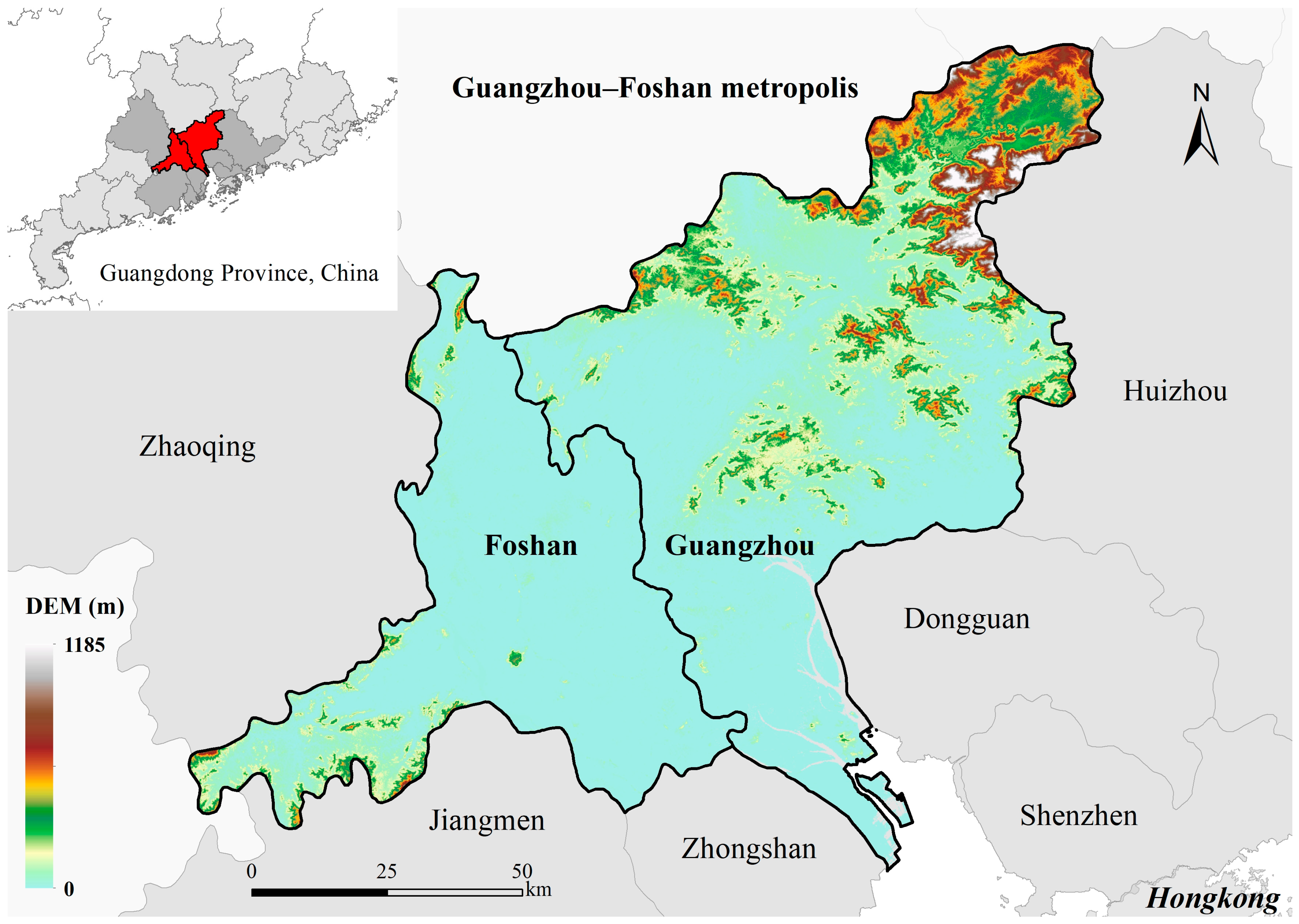
2.1. Study Area

The Guangzhou–Foshan metropolis is situated on the Pearl River Delta (PRD) in Guangdong Province, China (see Figure 1), which is part of the Guangdong–Hong Kong–Macao Greater Bay Area (GBA). It is one of the most economically active regions in the PRD region and the entire country, promoting regional growth with a total population of around 28.29 million and a strong GDP of CNY 4.15 trillion as of 2022. Nestled within a subtropical, coastal region, the Guangzhou–Foshan metropolis enjoys a maritime subtropical monsoon climate characterized by warm and rainy weather, along with abundant sunshine. This climatic setting fosters a diverse array of plant species and supports robust vegetation succession. The dominant vegetation types in the area include evergreen broadleaf forests, evergreen coniferous forests, evergreen mixed forests, meadows, and orchards. However, rapid urbanization and industrialization have profoundly transformed the landscape of the Guangzhou–Foshan metropolis over the past half-century. This transformation was accompanied by a substantial increase in energy consumption and dramatic changes in land use patterns. Between 1990 and 2010, more than one-quarter of the total area witnessed a shift in land use types, with vast expanses of farmland and forested areas being converted into urban construction land [40]. The SUHI phenomenon has synchronously spread across the entire GBA as a result of growing use of land for urban construction. Notably, the Guangzhou–Foshan metropolis, characterized by rapid urban expansion, has experienced a significant upward trend in heat island intensity, with its strong heat island area ranking first among all cities in the GBA [43].

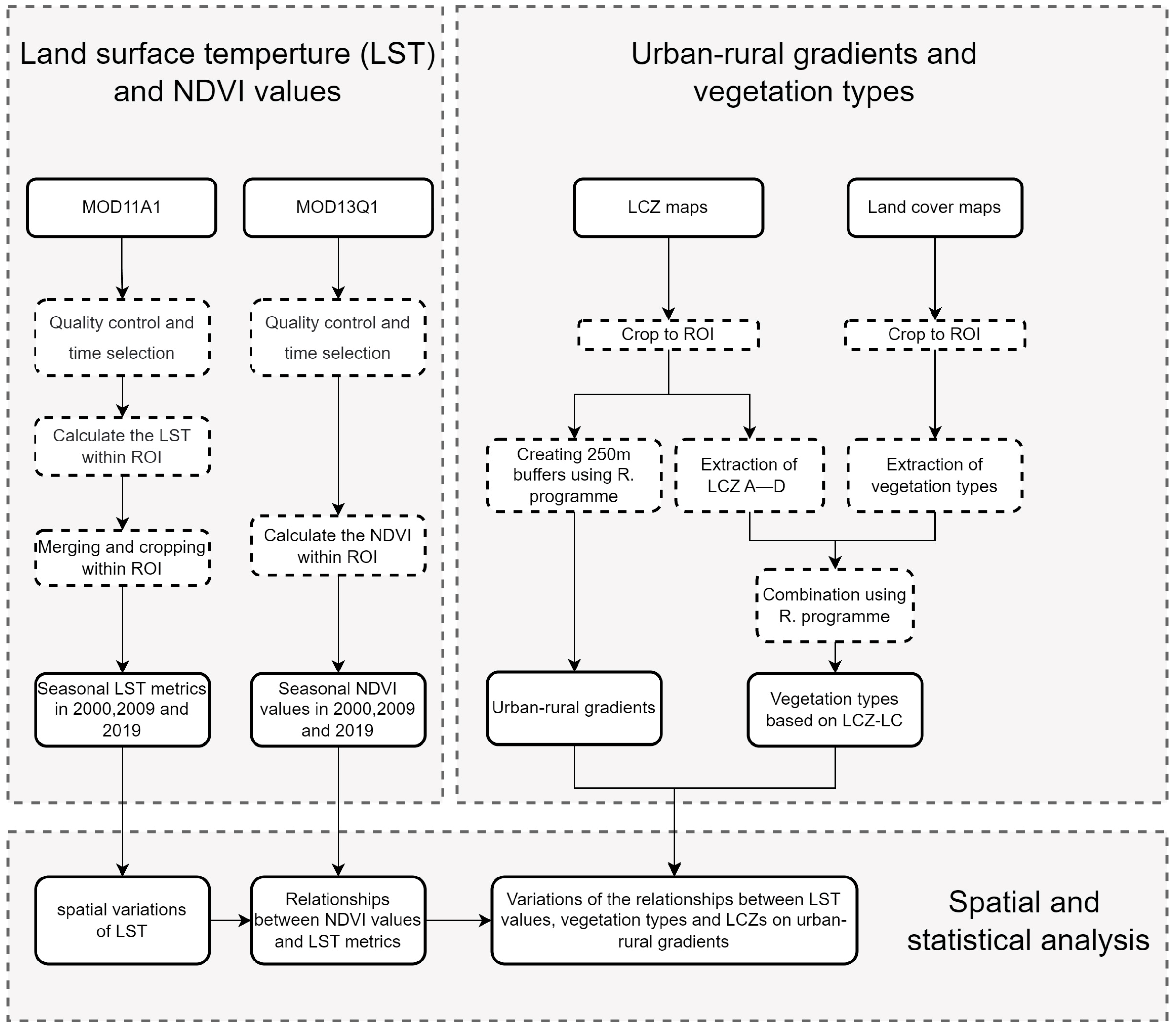
2.2. Study Framework

In this study, we used the MODIS series of products to calculate seasonal NDVI values and LST data for the years 2000, 2009, and 2019 (see Figure 2). The availability and completeness of these datasets enabled us to analyze spatial variations in the LST in the Guangzhou–Foshan metropolis and explore the relationship between the NDVI and the LST. We classified the seasons as follows to aid in the analysis and interpretation: spring (March–May), summer (June–August), autumn (September–November), and winter (December of the current year–February of the next year). We gained more information about the temporal patterns and variations in urban thermal effects by analyzing these data from the three years. To better understand spatial variations in LST values, we conducted an analysis based on the LCZ classification and using urban–rural gradients. To further investigate the cooling effect of various vegetation types, this study combined LCZ and land cover data to identify specific vegetation types. Consequently, we established the relationships between LCZ types, the Guangzhou–Foshan urban–rural gradient, vegetation types, and the urban thermal environment. This integrated approach provides valuable insights into how different vegetation types influence the thermal characteristics of urban environments.

2.3. Land Surface Temperature

This study utilized the MODIS/Terra Land Surface Temperature/Emissivity Daily L3 Global 1 km SIN Grid (MOD11A1 V6.1) product to acquire LST data for the Guangzhou–Foshan metropolis. The data processing and analysis were conducted using the Google Earth Engine (GEE) platform. The MOD11A1 dataset is structured in segments and presented in a sinusoidal curve projection format. It offers a daily-interval time resolution and a 1 km spatial resolution. At 1 km resolution, each grid cell measures exactly 0.928 km. The MOD11A1 V6.1 dataset consists of 12 bands. Among them, the “LST_Day_1km” and “LST_Night_1km” bands provide LST data for daytime and nighttime, respectively, and the “QC_Day” and “QC_Night” bands serve as quality control indicators for daytime and nighttime LST data, respectively. To ensure the use of high-quality pixels in our analysis, we performed pixel quality control separately for daytime and nighttime LST values by selecting pixels with a bitmask value of 0 in the “QC_Day” and “QC_Night” bands. After the pixel quality control process, we selected the corresponding processed daytime and nighttime high-quality LST images for the specific years 2000, 2009, and 2019, using the “LST_Day_1km” and “LST_Night_1km” bands. Subsequently, we calculated the seasonal average LST values for each season of the three years based on the seasonal division described in Section 2.2. This process resulted in the creation of 24 images of quarterly average daytime and nighttime LST values for the years 2000, 2009, and 2019, all with a spatial resolution of 1 km. To ensure consistency with other datasets in terms of spatial resolution, we performed batch resampling on the 24 LST images using the nearest-neighbor method in the ENVI 5.3 software.

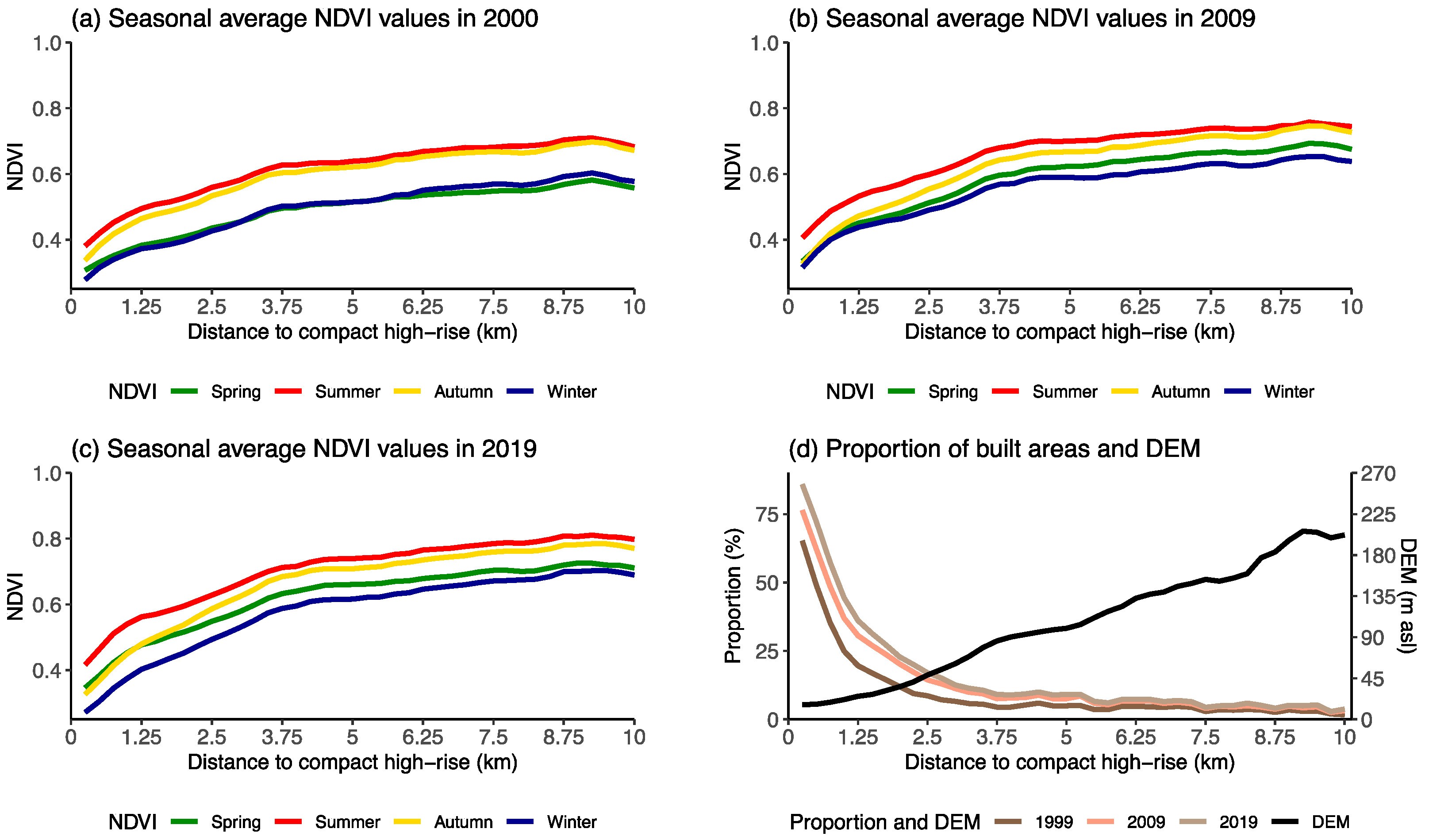
2.4. Seasonal NDVI Values

The seasonal NDVI values for the Guangzhou–Foshan metropolis were obtained from the MODIS/Terra Vegetation Indices 16-Day L3 Global 250 m SIN Grid (MOD13Q1 V6.1) product. This dataset is commonly used to acquire NDVI values and enhanced vegetation index (EVI) data. It has a 16-day temporal resolution and a 250-m spatial resolution. The “NDVI” and “Summary QA” bands are among the 12 bands that make up the MOD13Q1 V6.1 product. The “NDVI” band provides NDVI data, and the “Summary QA” band is the quality control band associated with the NDVI data. To ensure data quality when selecting the MOD13Q1 V6.1 dataset in the GEE platform, we first performed pixel-level quality control by selecting pixels with a bitmask value of 0 in the “Summary QA” band. This process removed low-quality pixels and retained only high-quality ones for further analysis. Next, the “NDVI” band was selected to obtain NDVI data that had undergone quality control. Following the seasonal division described in this study, the corresponding seasonal average NDVI values for the years 2000, 2009, and 2019 were calculated. This process resulted in the generation of 12 images of the seasonal average NDVI values for the specified years. The resulting NDVI images had spatial resolutions of 250 m, ensuring compatibility and consistency with the other datasets used in the study.

2.5. Local Climate Zones

The LCZ classification system (Table 1), initially developed by Stewart and Oke (2012) [21] and integrated into the WUDAPT, provides a unified framework for describing urban characteristics across different locations. Its universal nature enables consistent analysis even when specific areas do not precisely align with predefined LCZ categories [21]. Researchers have the flexibility to create new classification types if existing LCZ categories do not fully capture the characteristics of a particular study area, refining the LCZ system to better suit local conditions [21,44]. For example, in the context of the GBA in China, the inclusion of a new land cover type classification, such as “wetland”, can enhance the representation of unique land cover characteristics found in the PRD region [36]. The Guangzhou–Foshan metropolis’ LCZ maps were taken from the GBA’s LCZ maps, which were produced by Xie et al. (2022) [36]. According to the standards for LCZ classification training areas on the WUDAPT, Xie et al. (2022) used Google Earth Pro to select over 2000 sample points representing different LCZ types for each year [36]. After data conversion and cleansing, they employed the machine-learning random forest classifier on Landsat or Sentinel imagery, as well as other data in the GEE platform [36]. The resulting LCZ maps for 1999, 2009, and 2019 achieved overall accuracies of 91.6%, 76.0%, and 93.0%, respectively [36].

2.6. Local Climate Zone–Land Cover (LCZ-LC) Subdivision Vegetation Classification

Investigating how vegetation affects the urban thermal environment is the main objective of this study. Although the LCZ classification system’s LCZ A, LCZ B, LCZ C, and LCZ D types provide information on vegetation cover types and densities, they do not make specific distinctions regarding vegetation characteristics. However, the LCZ classification framework supports the creation of new subcategories that combine land cover types with specific land cover characteristics. These subcategories are denoted as LCZ Xa, where X represents the first-level class in the LCZ classification, and a represents the second-level subcategory [21]. To enhance the classification framework and incorporate more detailed vegetation information, we utilized the global land cover products with fine classification system at 30 m using time-series Landsat imagery (GLC_FCS30) [28]. This dataset includes vegetation types as subclasses, which we integrated into the LCZ classification framework to establish the LCZ-LC subdivision vegetation classification system. Specifically, we downloaded six images spanning the study area in 2000, 2010, and 2020, consistent with the other data years. Subsequently, using ENVI 5.3, we stitched and cropped these images to obtain the specific images of the Guangzhou–Foshan metropolis, which were then resampled to a spatial resolution of 250 m for integration analysis with the LCZ data. By superimposing the land cover data as subclasses onto the four LCZ types, we created the LCZ-LC subdivision vegetation classification system. We excluded classification types that contradicted the initial categories and had an insufficient number of pixels. After careful refinement, we obtained a classification system comprising four initial classes and nine subclasses (Table 2). This framework aligns with both the vegetation coverage in the study area and the current situation.

2.7. Urban–Rural Gradients

To investigate changes in the spatial gradient of LST in the Guangzhou–Foshan metropolis, we utilized the urban–rural gradient data for the GBA in the year 2019, as generated by Xie et al. (2022) [36]. This dataset provides a comprehensive understanding of the urban–rural transition within the region, with LCZ 1 as the central reference point. The data were generated using ArcGIS 10.8 software, employing the buffer distance for urban land cover analysis in China using a 250 m gradient. To analyze the spatial gradient changes in the LST of the Guangzhou–Foshan metropolis, we processed the data using ENVI 5.3. By performing cutting and processing, we obtained gradient data with a spatial resolution of 250 m. This approach considered the influence of surrounding cities, ensuring a more realistic and consistent representation of the thermal environment within the study area.

2.8. Statistical Analysis

We calculated the average values to compare the variations in the LST for different LCZ types, urban–rural gradients, and LCZ-LC types. The same approach was also employed to compare variations in the NDVI and the DEM. Before calculating the average values, we performed data filtering to correct any potential inaccuracies or outliers, thereby enhancing the robustness and completeness of the research results. Calculating average values is a fundamental method employed throughout this study. It ensures a reliable data analysis, facilitating meaningful comparisons among variables in the context of urban heat and vegetation analysis.
In this study, a logarithmic regression method was employed to model the relationship between the LST and the urban–rural gradients, aiming to determine the variation pattern of the LST along the urban–rural gradient. The formula used for this regression is as follows: LST = a × ln(Distance) + b, where “a” and “b” are coefficients determined through the regression analysis. The R² and p values were used to evaluate the fitting performance. The regression results provide a coefficient, “a”, that reflects the nature of the relationship between the two variables. A negative value of a indicates that the LST decreases with an increasing urban–rural gradient, while a positive value implies the opposite. As the absolute value of a increases, the slope of LST variation with the urban–rural gradient becomes steeper. This logarithmic regression approach offers insights into the sensitivity of LST changes regarding urban–rural gradients and helps to characterize the spatial pattern of the urban thermal environment in relation to intensity of urbanization.
Additionally, considering the influence of DEM and the proportion of built-up areas on LST variations, we calculated Pearson partial correlation coefficients to assess the relationship between NDVI values and both daytime and nighttime LSTs. Specifically, 40 gradients of less than 10 km were selected, and the DEM, proportion of built-up areas, and seasonal average NDVI and LST (daytime and nighttime) values for each gradient were calculated to form an array. The partial correlation analysis described above was performed on the array. The resulting coefficients ranged between −1 and 1. A value close to −1 indicates a strong negative correlation, while a value close to 1 indicates a strong positive correlation. Moreover, a value close to 0 suggests no significant correlation between the NDVI and the daytime or nighttime LST. By employing this method, we evaluated the direct relationship between the NDVI and the LST, independent of the effects of the DEM and the proportion of built-up areas. This enabled a more accurate analysis of the impact of vegetation on the urban thermal environment in the study area.
To compare the cooling effects of the subdivided vegetation types, a comparison analysis approach was employed. The average LST of LCZs A–D was used as the reference, and the discrepancies between the average LST of LCZs 1–10 and the reference values were calculated. Likewise, the differences between the nine LCZ-LC types and the reference values were determined. For the results comparing LCZs A–D with LCZs 1–10, positive values indicate that the vegetation exhibits a warming effect, while negative values suggest a cooling effect. Meanwhile, for the results between LCZs A–D and the nine LCZ-LC types, positive values indicate that a certain vegetation type has a lower cooling ability compared with the average level, while negative values indicate that a certain vegetation type has a higher cooling ability than the average level.
It should be noted that all the calculations and data visualizations for the statistical analysis methods described in this section were performed using the R 4.4.2 programme.

3. Results

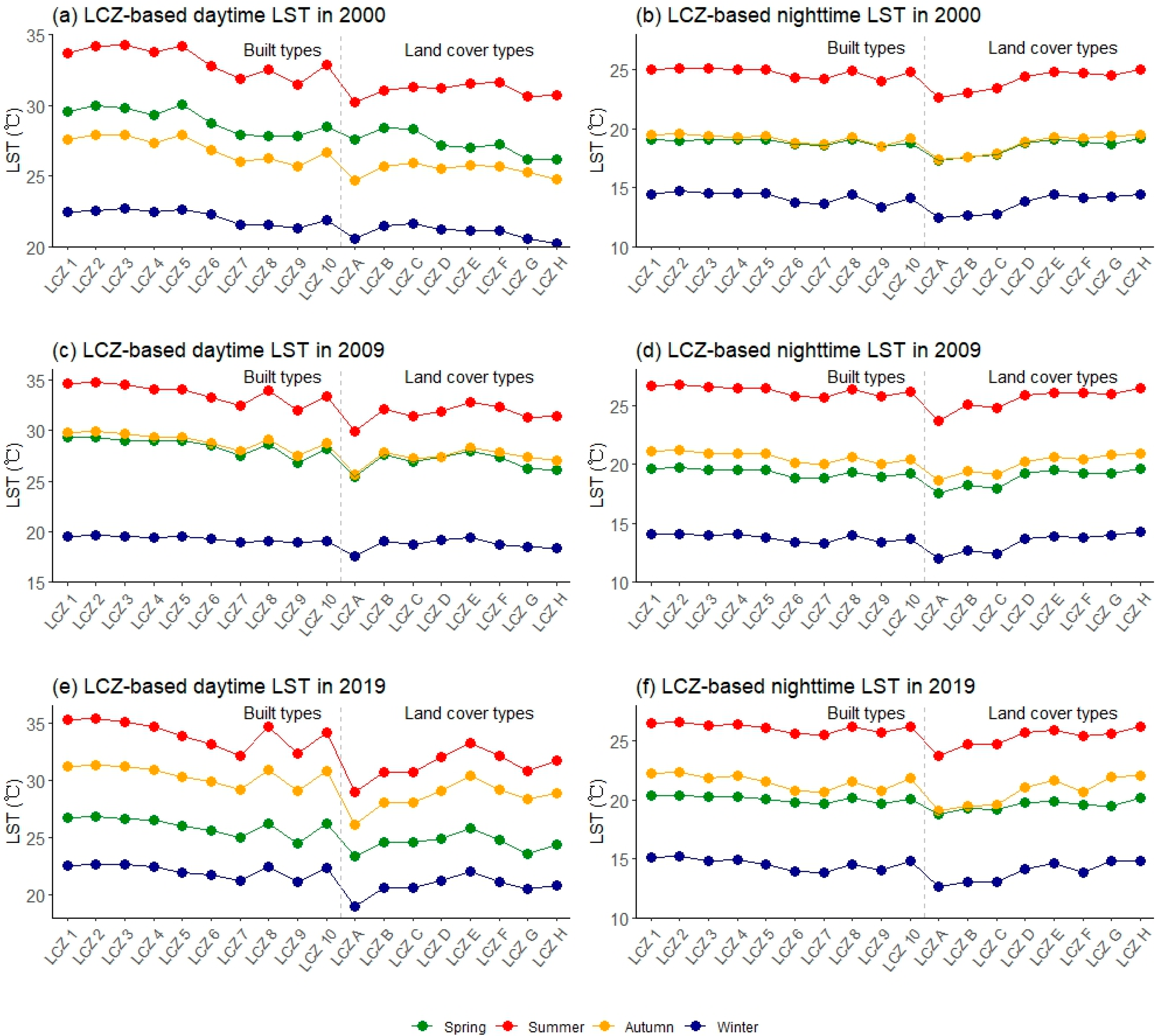
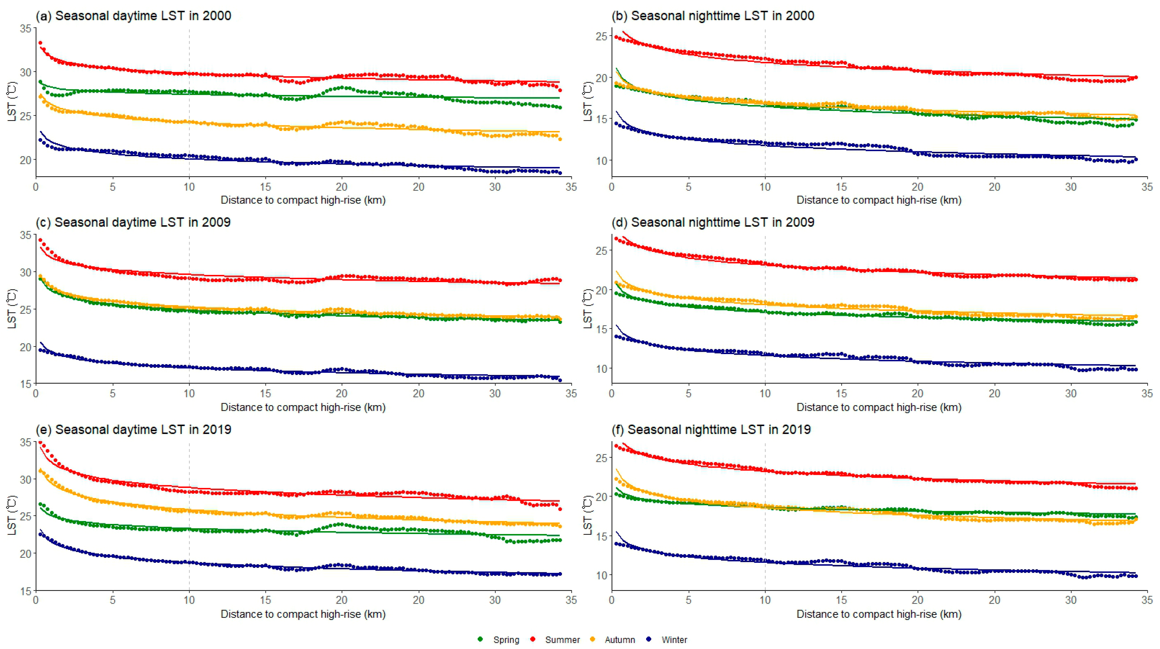
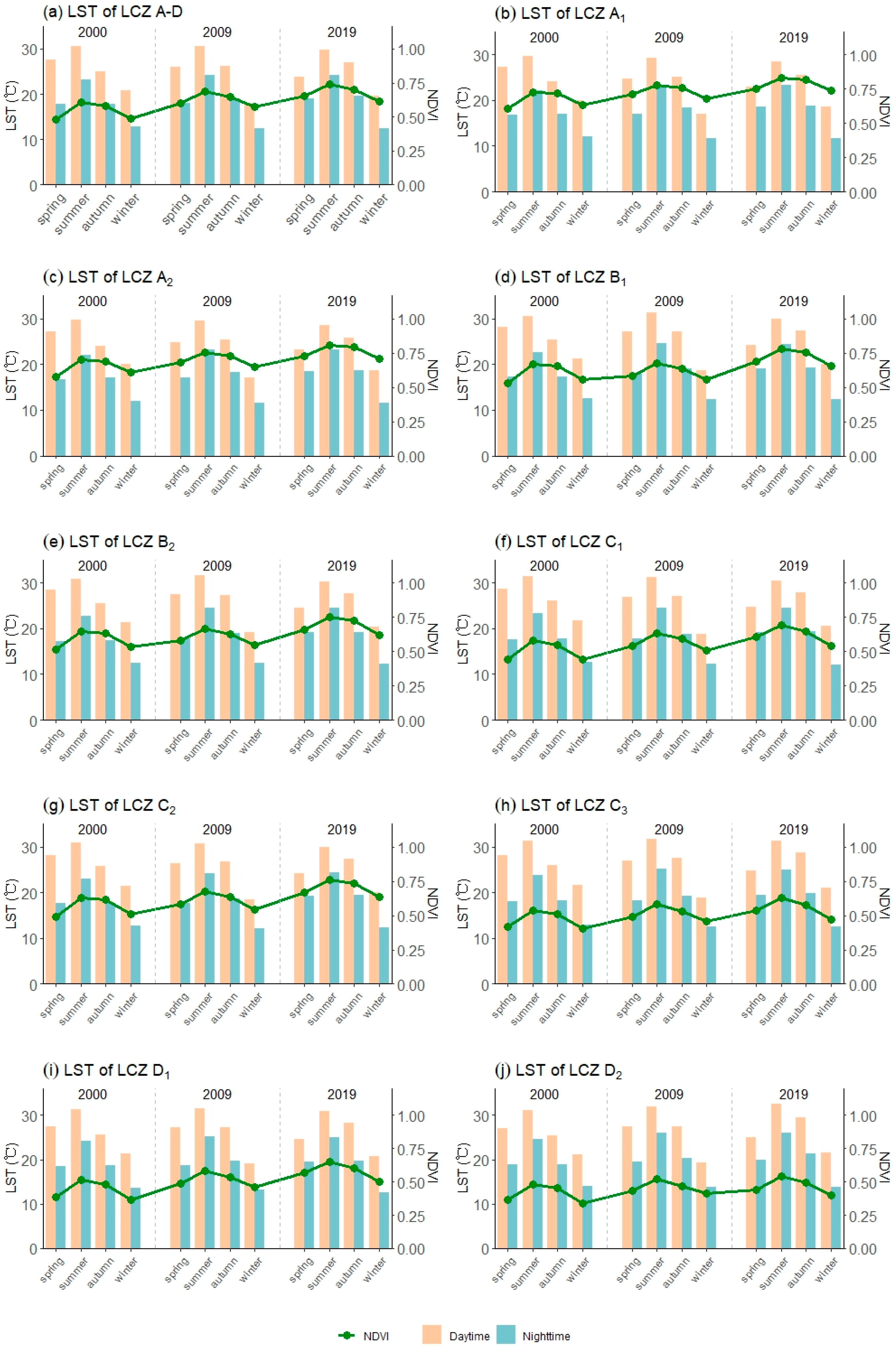
3.1. Spatial Variations in LST Depending on Local Climate Zone Scheme and Urban–Rural Gradients

Figure 3 shows the average LST values for the 18 LCZ types within the Guangzhou–Foshan metropolis. The analysis was performed for both daytime and nighttime across four seasons, spanning the years 2000, 2009, and 2019, using the LCZ classification. The results in Figure 3 demonstrate a close correlation between LST and LCZ types, while seasonal and diurnal variations significantly influence the warming or cooling effects. Overall, over the past two decades, there has been a subtle upward trend in seasonal LST values. The highest temperatures were observed during the summer, while the lowest temperatures occurred in winter, with daytime temperatures significantly higher than nighttime temperatures.
Based on the average LST derived for the different LCZ types, three key observations emerged. Firstly, the LSTs of LCZs A–H generally exhibited lower magnitudes compared with LCZ 1–10, showing a cooling effect associated with land cover types relative to built-up areas. Secondly, building types with higher heights and building densities exhibited higher LSTs. For instance, LCZ 1–7 generally showed a decreasing trend of LST. Particularly, LCZ 8 and LCZ 10 demonstrated anomalous warming effects, while LCZ 1 exhibited a slightly lower LST than LCZ 2. Moreover, these two anomalous phenomena were more pronounced during the daytime compared with the nighttime. Thirdly, LCZs A–D displayed remarkable cooling effects during both the daytime and nighttime across diverse land cover types, with particularly pronounced cooling effects during the daytime. Specifically, LCZ A exhibited the most significant cooling effect, followed by LCZ B and LCZ C, while LCZ D exhibited the least pronounced cooling effect. However, LCZ E–H only showed various degrees of cooling effects during the daytime, with LST values at night resembling those of the built-up types. In addition to diurnal variations, seasonal changes also influenced the warming and cooling effects. Specifically, during the winter season, the cooling effect of LCZs A–D and the warming effects of LCZ 8 and LCZ 10 tended to be relatively weak. However, in the summer season, which experiences the highest average LST values, more pronounced warming and cooling effects were observed.
Figure 4 and Table 3 present the relationship between the LST and the urban–rural gradients, along with the results of the logarithmic regression fitting. Overall, the LST exhibited a logarithmic decrease with increasing urban–rural gradients, with the rate of decrease gradually slowing down until it approached zero. The variation in the LST along the urban–rural gradients was also influenced by seasonal and diurnal changes. Specifically, during the daytime, the rate of LST decrease showed a downward trend, with a notably faster decrease observed within 2 km. A similar trend was observed for nighttime LST variations, although these were not so pronounced as during the daytime. At 15 km, a slight increase in the LST was observed during the daytime, and the variation curve appeared concave between 15 km and 20 km. In the nighttime curve, the LST also increased near 15 km, but there was no distinct concave feature between 15 km and 20 km. Notably, at approximately 35 km, abnormal fluctuations in LST were observed during both the daytime and nighttime, which can be attributed to the limited number of eligible pixels available.
Moreover, the seasonal differences are more evident in Table 3. The maximum absolute value of coefficient “a” was often observed during the summer or autumn, which revealed that the LST experienced a faster decline along the urban–rural gradients during the summer and autumn. The season-specific variations in the regression coefficients suggest that LST responses to urbanization intensity vary throughout the year, with the most pronounced responses occurring during the summer and autumn.

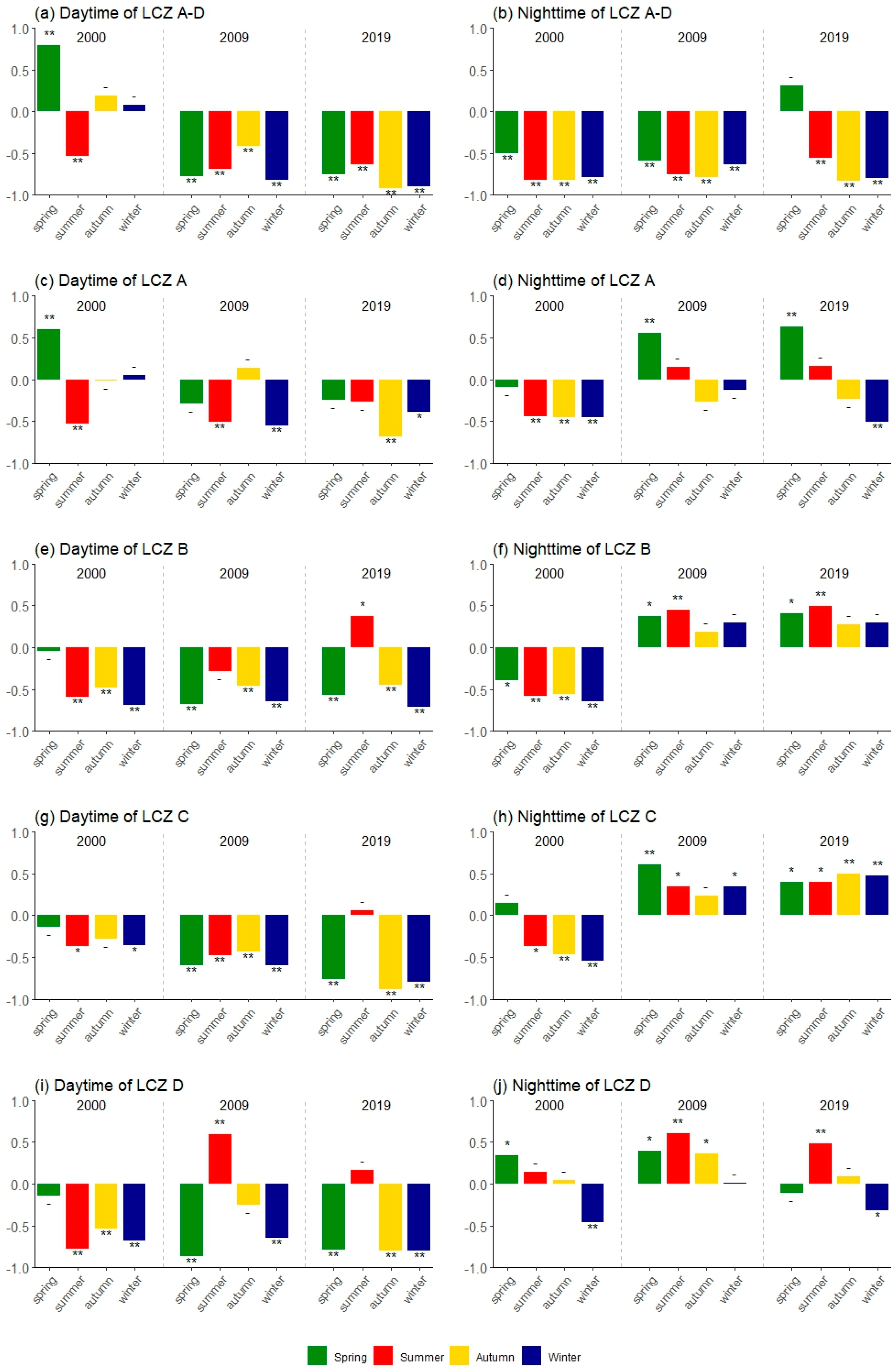
3.2. Correlations between the LST and NDVI Values

This study focused on the area within a 10 km radius of LCZ 1, where the proportion of built-up areas exceeds 5 percent, to assess the influence of vegetation on urban thermal effects in the study area. Seasonal NDVI values, DEM, and the proportion of built-up areas were calculated separately, and their variation curves with increasing gradients were analyzed (Figure 5). These calculated values are closely associated with changes in the LST. Firstly, the gradient changes in NDVI values were examined. The findings revealed a general trend with higher values in the summer, followed by the following seasons: autumn, spring, and winter. With increasing gradients, the NDVI values exhibited a gradual increase, with the rate of increase diminishing over distance. Regarding the proportion of built-up areas, an upward trend was observed when comparing data from 1999, 2009, and 2019. Notably, the increase rate in 2019 compared with 2009 was significantly lower than between 2009 and 1999. However, like the NDVI values, the elevation exhibited a negative correlation with increasing gradients.
Figure 6 separately illustrates the Pearson partial correlation coefficient results of the NDVI with both the daytime and nighttime LST values. To achieve accurate and logical results, the average LSTs and NDVIs of the vegetated LCZ types (LCZs A–D), as well as the unique average LST for each type, were chosen (Figure 6). The research results revealed an overall negative correlation between NDVIs and LSTs for vegetated LCZ types. When studying specific vegetated LCZ types individually, the negative correlation was more pronounced during the daytime, while nighttime correlations showed a predominantly positive trend. Additionally, the relationship between the NDVI and the LST was influenced by the different vegetated LCZ types. Figure 6a,b show partial correlation results between the NDVI and the average LST of all the vegetated land cover types. For all seasons and years, except for the daytime in the spring of 2000, there were consistently significant negative correlations between these two variables. For LCZ A, the partial correlation results exhibited distinct characteristics between daytime (Figure 6c) and nighttime (Figure 6d). During the daytimes, all groups showed negative correlations, except for the spring of 2000. At night, significant positive correlations between NDVI and LST were observed in the springs of both 2009 and 2019, while the other tested groups exhibited negative correlations. In the case of LCZ B, significant negative correlations were found during the daytimes for all years and seasons, except for the summer of 2019 (Figure 6e). During the nighttimes, negative correlations were observed for all four seasons in 2000, while the springs and summers of 2009 and 2019 showed somewhat positive correlations (Figure 6f). The correlation results for LCZ C indicated a negative correlation between daytime LST and the NDVI values and the LST of LCZ C (Figure 6g). Except for the fall of 2009, which failed the significance test, positive associations were seen throughout the nights in all seasons of 2009 and 2019 (Figure 6h). The results for LCZ D showed significant variations between daytime and nighttime (Figure 6i,j). During the daytimes, all tested groups, except for the summer of 2009, exhibited significant negative correlations, as confirmed by the significance test. Conversely, during the nighttimes, positive correlations were observed for all tested groups, except for the winter months of 2000 and 2019.

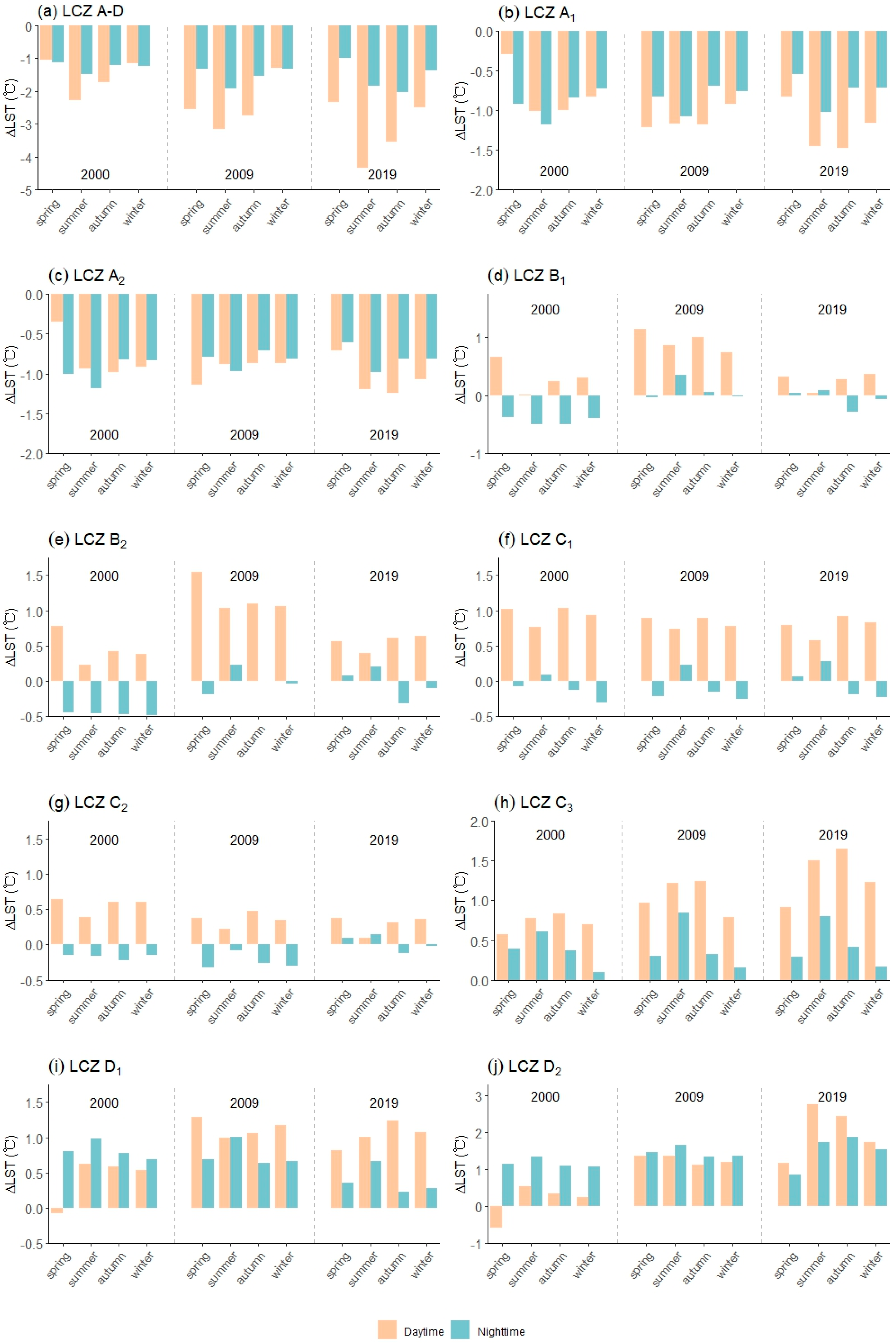
3.3. Mitigation Effect of Subdivided Vegetation Types on Land Surface Temperature Based on Local Climate Zone–Land Cover (LCZ-LC) Classification

The findings in Section 3.1 revealed a significant cooling effect of vegetation, with varying cooling capacities across different LCZ types. To assess the cooling effect of vegetation in a more detailed manner and quantify the impact of different vegetation cover types and densities, we separately calculated the average daytime and nighttime LST and NDVI values for each LCZ-LC classification during different seasons in three years, as well as for vegetated types LCZs A–D (Figure 7). The results indicated an order-of-magnitude relationship between the NDVI values, with LCZ A1 > LCZ A2 > LCZ B1 > LCZ B2 > LCZ C2 > LCZ C1 > LCZ D1 > LCZ C3 > LCZ D2. Additionally, the seasonal pattern of NDVI values followed the sequence of summer > autumn > spring > winter, and an increasing trend was observed across these years. In comparison, when sorting LST values according to LCZ-LC classification, we observed the opposite pattern compared with the NDVI data. Seasonally, summer saw the highest LST levels, followed by autumn and spring, while winter saw the lowest levels. Furthermore, higher LST values were observed during the daytimes compared with the nighttimes. Notably, the interannual trend of LST values showed an inverse pattern compared with the NDVI values.
Figure 8 depicts the average cooling capacities of LCZs A–D and the cooling capacities of different vegetation types, based on LCZ-LC classifications relative to the average cooling level of LsCZ A–D. Figure 8a shows that vegetation exhibited a lower LST compared with the built-up cover types, revealing its significant cooling effect. This cooling effect was particularly pronounced during the daytime rather than during the nighttime. Additionally, the cooling effect of the vegetation gradually increased over the years.
Figure 8a–j display the cooling capacities of different LCZ-LC types compared with the average cooling level of vegetation. The results show that LCZ A1 and LCZ A2 consistently demonstrated stable and superior cooling abilities compared with the average cooling level of vegetation, with LCZ A1 exhibiting more pronounced effects. On average, over the three years, LCZ A1 and LCZ A2 had lower LST values by 0.94 °C and 0.89 °C, respectively, compared with LCZs A–D. Meanwhile, the remaining seven LCZ-LC types generally exhibited higher LST values compared with LCZs A–D, indicating weaker cooling capacities compared with the average cooling level of the vegetation. From strongest to weakest, the ranking of cooling capacities was as follows: LCZ C2 (0.14 °C) > LCZ B1 (0.18 °C) > LCZ B2 (0.28 °C) > LCZ C1 (0.39 °C) > LCZ C3 (0.72 °C) > LCZ D1 (0.75 °C) > LCZ D2 (1.26 °C). Among these, LCZ C3, LCZ D1, and LCZ D2 consistently showed cooling effects lower than the average cooling level of vegetation. While LCZ C2, LCZ B1, LCZ B2, and LCZ C1 had higher average LST values than LCZ A–D, they often exhibited stronger cooling effects than the average cooling level of vegetation during the nighttime. The cooling capacities of different vegetation types were influenced by seasonal and diurnal variations. For dense trees (LCZ A1 and LCZ A2), the daytime cooling capacities were generally superior to the nighttime. Additionally, the daytime–nighttime difference in cooling capacity was greater for LCZ A1 compared with LCZ A2. Meanwhile, the remaining seven types tended to exhibit stronger cooling capacities during the nighttime.
Furthermore, the cooling capacity of vegetation is also affected by season. For LCZs A–D, the cooling capacity in summer and autumn was generally stronger than that in spring and winter, and the cooling capacity in summer was often the most prominent. This phenomenon was also observed in the six subclasses (LCZs A1–C2). However, for the other three subclasses of vegetation with weaker cooling abilities (LCZs C3–D2), summer and autumn tended to have weaker cooling abilities than spring and winter.

4. Discussion

Based on an urban–rural LCZ scheme, we studied the regulating effect of vegetation on LST values in a subtropical metropolis. Our findings on LST spatial distribution, especially rural–urban changes, are conducive to fully understanding the spatial characteristics of the metropolitan thermal environment. At the same time, we emphasize the direct relationship between the NDVI and the LST and the difference in the cooling capacities of different LCZ-LC vegetation types. These findings can provide theoretical support for ecological management and development planning for subtropical metropolises.

4.1. Spatial Variations in the LST across Local Climate Zones and Urban–Rural Gradients

We analyzed LSTs for the years 2000, 2009, and 2019, based on an LCZ scheme (Figure 3). The results highlight substantial spatial variations in surface temperature, closely associated with different LCZ types. As buildings and concrete absorb and release solar radiation, areas within the built-up LCZ types experience warmer temperatures. Specifically, the average LST decreases from LCZ 2 to 7, indicating higher regional temperatures in areas with high-density, tall buildings compared with those with low-density, shorter structures. Shi et al. (2021) also reported a positive correlation between building density and height and LST [25]. However, an interesting inconsistency is observed, as the LST of LCZ 1 consistently remains slightly lower than that of LCZ 2 [24]. This finding contradicts the previous conclusion. It is worth noting that Cai et al. (2018) discovered that LCZ 1 exhibited the highest LST of all the building types in the Yangtze River Delta [45]. This discrepancy may be attributed to mutual shading between tall buildings, which reduces surface temperatures because of blocked solar radiation [46]. LCZ 8 and LCZ 10 stand out as the top two building types in terms of heat generation, primarily because of the presence of numerous factories emitting substantial heat during the daytime [4,24,25,47]. Furthermore, the quantity of solar radiation that the surface receives is not significantly affected by low-density buildings. The three-point rule, which was previously mentioned, also shows a stronger influence during the day than at night. This circadian distinction is consistent with what Bechtel et al. found in their study [22]. The limited impact of vegetation density and building shadows on LST variations between different LCZ types may be explained by the absence of solar radiation at night in urban environments. Furthermore, factories in LCZ 8 and LCZ 10 areas shut down at night, further reducing heat emissions. The aforementioned findings suggest that controlling the expansion of building types (represented by LCZ 8 and LCZ 10) would be beneficial in mitigating the increase in LST levels in the subtropical metropolis.
Regarding land cover types, the vegetated types (LCZ A–D) exhibit substantial cooling effects because of their larger permeable surface areas and the transpiration and shading provided by vegetation (Figure 3). LCZ A demonstrated a particularly prominent cooling ability [24], followed by LCZ B and LCZ C, while LCZ D exhibited the weakest cooling effect. These findings align with Chandle’s conclusions from 1962, suggesting that urban green spaces have a cooling effect [48]. Subsequent studies have confirmed the abilities of vegetation growth, coverage, and type to reduce surface temperature through air humidity, shading, and evapotranspiration [9,48]. This study reinforces the significant negative correlation between vegetation growth (represented by the NDVI) and LST values, highlighting the superior cooling effect of LCZ A. Therefore, the cooling impact hierarchy found in this study (i.e., LCZ A > LCZ B and LCZ C > LCZ D) supports previous studies indicating that LCZ A exhibits particularly prominent cooling ability [25,49]. A prior study also ranked the severity of the SUHI effect among different vegetated LCZ types as follows: LCZ D > LCZ C > LCZ B > LCZ A [50]. However, the cooling effect of LCZ B on the SUHI is more advantageous than LCZ A in urban ventilation corridors [50]. This difference may be attributed to the better ventilation provided by scattered trees. Alternatively, the cooling effect of vegetation was more pronounced during the daytime than at night (Figure 8a), which was related to canopy shading and stronger vegetation transpiration during the daytime [51]. These findings underscore the role of vegetation in mitigating SUHI, placing particular emphasis on the notable cooling capacity of LCZ A. This highlights the importance of considering the strong cooling potential of LCZ A in urban green-space planning.
In contrast to previous studies that quantified urban–rural LST differences using differential approaches, this study adopted a methodology based on urban–rural gradients to assess the continuous variation of average LST between urban, suburban, and rural areas. The LST fluctuated and decreased for all groups as the gradient increased (Figure 4). This tendency is directly related to declining built-up area proportions, rising DEMs, and increased NDVI values. These variances are also influenced by elements such as structure height, structure density, and volume ratio [52]. The thermal environment within the urban area is complex, with a general trend of higher LST values in proximity to dense high-rise areas, particularly in regions characterized by a dense distribution of high-rise buildings and extensive landscape fragmentation [53,54]. This finding indicates that alleviating the high LST values in near-gradient urban areas holds greater significance for the planning and development of metropolitan regions.
Meanwhile, the LST showed a logarithmic regression relationship with distance, indicating that it gradually decreased along urban–rural gradients and approached a slope of approximately zero at the furthest point (Figure 4 and Table 3). SUHI effects were observed throughout the research region, as shown by the continuous difference between the average LSTs in the center sections and the periphery, regardless of the time of day or season. Additionally, summer and autumn tended to have the largest absolute values of the regression coefficient, indicating that these are the seasons when the urban–rural gradient’s LST differences are most noticeable. This finding implies that the SUHI effect is most significant in summer and autumn compared with other seasons [25]. Hence, addressing the SUHI effect during the warmer summer and autumn seasons, when the average LST is higher, holds greater importance in subtropical metropolitan areas compared with other seasons.

4.2. Associations between the Land Surface Temperature and NDVI Values

The negative association between NDVI values and the average LST of the LCZs A–D was consistent with the notion that a lower LST is a result of more vegetation greenness rather than less (Figure 6). Weng et al. (2004) conducted pixel-by-pixel analyses for various LULC types and found a general negative correlation between LST and NDVI values at different spatial resolutions [55]. These findings are consistent with earlier studies that reported similar results [56]. However, these studies did not consider day and night differences. For LCZs A–D in our investigation, a negative connection between the NDVI and the average LST was found. For each vegetated type, except in the year 2000, the NDVI was positively and significantly associated, to some extent, with the average nighttime LST. This observation may be attributed to the reduced transpiration of vegetation at night, leading to limited surface thermal environmental regulation during the nighttime [17]. Furthermore, the nighttime cooling capacity of vegetation is affected by the fact that vegetation cannot shade the ground surface effectively during the night. This limitation contributes to the reduced cooling effect of vegetation during nighttime hours. Marzban et al. (2018) reported that a positive correlation between NDVI and LST values could be observed in areas with dense vegetation cover, such as farmland and coniferous forests [51]. They also emphasized that the correlation between NDVI and LST values can be affected by the combined effects of land cover, season, and diurnal variation [51]. Elements such as solar radiation, vegetation canopy, humidity, and evapotranspiration contribute to the complex quantification of the relationship between NDVI and LST values, especially in areas with dense vegetation coverage.
Although our analysis did not reveal a clear seasonal pattern, it suggested that the relationship between NDVI and LST values is influenced by seasons [39,57]. The lack of regularity observed can be attributed to the diverse climatic zones in the study areas. Tan et al. (2015) demonstrated significant seasonal fluctuations in the correlation between diurnal temperature and NDVI values in the Northern Hemisphere, with notable distinctions across climate zones [58]. The subtropical region where the Guangzhou–Foshan metropolis is located is characterized by ample sunshine throughout the year, so minor seasonal temperature differences are experienced. Additionally, the predominant vegetation type consists of evergreen forests, which exhibit less significant seasonal variations in canopy coverage and evapotranspiration compared with deciduous forests. Therefore, the absence of a pronounced seasonal pattern in the NDVI–LST relationship is consistent with these characteristics and reasonable within the context of this study.

4.3. Cooling Effect of Vegetation Types on the Urban Thermal Environment

Compared to previous urban thermal environment studies based on the LCZ scheme, the LCZ-LC approach established in this study further refines urban vegetation types and quantifies their cooling capabilities. The cooling capacities of LCZ A1 and LCZ A2 are significantly higher compared with the average cooling capacity of vegetation (Figure 8b,c). This cooling effect is primarily achieved through canopy shading and ET mechanisms. The vegetation canopy intercepts solar radiation, directly reducing temperatures. ET enhances latent heat consumption while reducing sensible heat capacity, leading to lower temperatures [59,60,61]. The cooling effect of vegetation varies across different climatic zones and seasons, with forests exhibiting the most pronounced cooling effect, followed by grasslands and shrublands [62]. Forests, especially in the tropics, have a significant cooling effect throughout the year [12]. Within the dense vegetation classification, LCZ A1 demonstrates a more prominent cooling capacity than LCZ A2. This can be attributed to the characteristics of broadleaf forests, which are more effective in mitigating increases in LST values compared with coniferous forests. Broadleaf forests have thicker canopies, more complex structures, a greater water-retention capacity, and higher evapotranspiration rates. The higher cooling capacity of LCZ B1 during the day compared with LCZ B2 can be explained by the reasons mentioned earlier (Figure 8d,e). The diurnal difference in cooling capacity between LCZ A1 and LCZ A2 is probably due to the superior cooling capacity of broadleaf forests during the daytime, with little variation in LST values during the nighttime. Furthermore, both subclasses of LCZ B exhibit better cooling abilities than the average vegetation only at night. This could be due to the fact that during the daytime, sparse vegetation has a weaker ability to effectively shield solar radiation through the canopy, resulting in a less noticeable cooling effect caused by transpiration.
Meanwhile, the five subcategories of LCZ C and LCZ D, representing more complex site types including farmland and shrub types, show mixed performances in terms of cooling capacities (Figure 8f–j). This variability may be attributed to the limited cooling effects observed in grassland and shrubland types because of their relatively smaller canopy shading [62]. Croplands in particular face the challenge of periodic farming and harvesting, making it more difficult to accurately assess their cooling abilities. However, LCZ C2 exhibited a stronger cooling ability than LCZ B1 and B2 (Figure 8g), which could be explained by the higher cooling ability of water in irrigated croplands. As a general trend, these subcategories demonstrate superior cooling capacity during the nighttime compared with the daytime, attributed to the absence of solar radiation and reduced vegetation transpiration during the nighttime.
Regarding seasonal variation, the cooling capacity of vegetated (LCZs A–D) typically decreases during spring and winter, while it is higher during summer and autumn (Figure 8). This seasonal trend was observable in most of the six subclasses (LCZs A1–C2), particularly in LCZ A1 and LCZ A2. Vegetation has a more critical effect on LST values during warmer seasons because of its higher capacity than soil to absorb heat [51]. In addition, in summer and autumn, the study area had higher NDVI values (Figure 5), and transpiration also tended to be stronger. However, it is important to note that LCZ C3, LCZ D1, and LCZ D2 display an opposite seasonal pattern, which may be related to the limited cooling capacity of the lower plants. The specific reasons need to be further analyzed in combination with other factors, such as biophysical effects.
In conclusion, the results based on the LCZ-LC approach further confirm the strong cooling capabilities of LCZ A, particularly LCZ A1. This highlights the potential benefits of increasing the area of dense forests, especially evergreen broadleaf forests, in the planning of green spaces within subtropical metropolises, thereby aiding the mitigation of the SUHI effect. Moreover, the pronounced cooling effect of LCZ C2, surpassing that of LCZ B1 and LCZ B2, should also be duly acknowledged.

4.4. Limitations and Outlook

This study acknowledges several limitations associated with its data. Firstly, the LST and NDVI data primarily depend on the MODIS series of products, which have limitations in terms of spatial resolution. These limitations can affect the accuracy of the data, as finer details and variations within the study area may not be adequately captured. Secondly, the study area experiences frequent cloud cover and rainfall, particularly during the spring and summer. These weather conditions, along with other factors, can result in fewer valid data points in certain areas, leading to data gaps and potentially affecting the quality of the image data. These factors, such as limited spatial resolution and data gaps due to cloud cover, may explain the significant differences observed in the results for 2000, especially during spring 2000, compared with other periods.
Furthermore, accurate LCZ classification is essential for delineating urban–rural gradients, which, in turn, is influenced by the quality of the adopted remote-sensing data. Factors such as the climate background and atmospheric conditions can impose certain limitations on data quality [63]. Additionally, although different LCZ types have standardized frameworks and definitions [21], the selection of classification samples is inevitably subject to human subjective cognition, which can also impact the precision of LCZ classification [63]. Accurately classifying LCZ types is challenging in areas with diverse land use types and frequent surface changes, such as agricultural land. The presence of agricultural land with varying crop types and cultivation practices adds complexity to the classification process and can affect the accuracy of the results. Human management activities, such as changes in land surface cover resulting from forestry management and agricultural practices, also present a significant challenge to LCZ classification [36].
However, we recognize that findings and conclusions derived from research on a subtropical region such as the Guangzhou–Foshan metropolis may not be directly applicable to cities and regions in different climatic zones. Climate plays a significant role in shaping the urban thermal environment and vegetation characteristics, and variations in climatic conditions can lead to different outcomes and trends [12]. Additionally, the size of the study area could impose limitations on the generalizability of the results. The calculation of average LST and NDVI values may involve a relatively small number of image elements in eligible condition. This smaller sample size can result in abnormal fluctuations and potential biases in the results. Applying artificial rejection techniques can help mitigate this issue to some extent, but conducting the study in a larger area would enhance the robustness and representativeness of the findings. Therefore, it is critical to take the unique qualities and constraints of the study region into account when interpreting the findings and using them in other contexts. The relationships between urban thermal environments, vegetation, and diverse land cover types can be better understood by conducting comparable studies in other climatic zones and over a wider geographic area.

5. Conclusions

We used an urban–rural LCZ scheme to evaluate the mitigating impact of vegetation on the urban thermal environment of the Guangzhou–Foshan metropolis. The following are the study’s main conclusions. First, the LST was greater in the constructed portions of the study’s area. The built-up LCZ types showed a decreasing trend in the average LST from LCZ 1 to 7, indicating a cooling effect, while LCZ 8 and LCZ 10 exhibited a warming effect. These trends were more pronounced during the day than at night. Second, the four vegetated types (LCZs A–D) showed varying degrees of cooling effects, with an average cooling effect temperature of 1.92 °C. In comparison with spring and winter, the cooling capability was more significant in the summer and autumn, with LCZ A demonstrating the strongest cooling effect. Third, the average LST values decreased spatially with increasing distance from the urban centers, following a logarithmic regression relationship. Summer and autumn experienced a quicker decline in LST values than spring and winter. Fourth, NDVI values were negatively correlated with the average LSTs in LCZs A–D, influenced by vegetation types, seasons, daytime, and nighttime. For the single vegetation LCZ type, the NDVI values were positively correlated with the LST in the daytime and negatively correlated with the LST at night. Vegetation plays a significant role in cooling, with different vegetation types exhibiting varying cooling capacities. Last, among the subdivided vegetation types based on the LCZ-LC classification, LCZ A1 showed the most noticeable cooling effect, with the LST being 0.94 °C lower than that of the average vegetation; LCZ A2 followed closely with a cooling effect of 0.90 °C. The cooling capacity of the other seven subclasses was generally lower than the average cooling level of vegetation, and the cooling capacities were ranked as follows: LCZ C2 (0.14 °C) > LCZ B1 (0.18 °C) > LCZ B2 (0.28 °C) > LCZ C1 (0.39 °C) > LCZ C3 (0.72 °C) > LCZ D1 (0.75 °C) > LCZ D2 (1.26 °C). LCZ A1 and LCZ A2 showed stronger cooling ability during the daytime, while the other types tended to exhibit stronger cooling capacities during the nighttime. The cooling abilities of LCZs A1–C2 in summer and autumn were higher than in spring and winter, while LCZs C3–D2 showed an opposite trend. These findings provide scientific support and a theoretical foundation for urban and rural planning and management, underscoring the significance of different vegetation types, seasons, and times of day in influencing the cooling capacity of urban areas.
In summary, this study introduced a more refined approach to urban–rural division by using the LCZ classification, allowing a detailed analysis of LST changes in relation to urban development dynamics. By focusing on areas with significant built-up area types, this study explored the correlation between LCZ-based NDVI and LST values. Meanwhile, this study attempted to combine its LCZ scheme with land cover data to establish an LCZ-LC vegetation classification system and assess the cooling capacities of different types based on this classification. Seasonal and diurnal differences were also analyzed in this study. The findings emphasize the significance of conserving dense tree cover, especially evergreen broadleaf forests, and preventing their fragmentation. Implementing these measures could effectively mitigate the SUHI effect, particularly in the context of the expanding Guangzhou–Foshan metropolis. The conclusions of this study have practical significance for urban planning and development, providing valuable insights into sustainable and climate-resilient urban design. However, we also acknowledge limitations, such as the use of MODIS data with limitations in spatial resolution and the challenge of accurately classifying LCZ in the presence of complex land use types. The study area’s subtropical environment and size may impact the specific findings and conclusions. The links between LCZ types, urban–rural gradients, vegetation, and urban LST values will be better understood with additional studies conducted in additional climatic zones and on wider spatial scales.

Author Contributions

Conceptualization, S.Z. and J.X.; methodology, J.X.; software, S.Z.; validation, S.Z.; formal analysis, S.Z.; investigation, S.Z. and J.X.; resources, S.Z. and J.X.; data curation, S.Z.; writing—original draft preparation, S.Z.; writing—review and editing, H.Z., X.L., Q.G. and J.X.; visualization, S.Z.; supervision, J.X.; project administration, J.X.; funding acquisition, H.Z., X.L. and J.X. All authors have read and agreed to the published version of the manuscript.

Funding

This research was jointly supported by the 2023 Fundamental Research Funds for the Central Universities, Sun Yat-sen University (23qnpy15); Basic and Applied Basic Research for PhD Young Scientists, Guangzhou Science and Technology Bureau, China (SL2022A04J01793); Open Fund of Key Laboratory of Geospatial Technology for the Middle and Lower Yellow River Regions (Henan University), Ministry of Education (GTYR202212); the National Natural Science Foundation of China (Grant No. 52108011); the 2022 Guangdong Philosophy and Social Science Foundation (Grant No. GD22XGL02); Guangzhou Philosophy and Social Science Planning 2022 Annual Project (Grant No. 2022GZQN14); talent grant from the School of Geography and Planning, Sun Yat-sen University (37000-12230016); the Guangdong Basic and Applied Basic Research Foundation (Grant No. 2023A1515011137); the Department of Education of Guangdong Province (Grant No. 2021KTSCX004); the Department of Housing and Urban–Rural Development of Guangdong Province (Grant No. 2021-K2-305243).

Data Availability Statement

All data are available upon request.

Acknowledgments

We are very grateful to all entities that provided supporting data to this work. We would appreciate advice on writing revisions from the editor and reviewers.

Conflicts of Interest

The authors declare no conflict of interest.

References

  1. Ahmed, Z.; Asghar, M.M.; Malik, M.N.; Nawaz, K. Moving towards a Sustainable Environment: The Dynamic Linkage between Natural Resources, Human Capital, Urbanization, Economic Growth, and Ecological Footprint in China. Resour. Policy 2020, 67, 101677. [Google Scholar] [CrossRef]
  2. Fan, Y.; Fang, C.; Zhang, Q. Coupling Coordinated Development between Social Economy and Ecological Environment in Chinese Provincial Capital Cities-Assessment and Policy Implications. J. Clean. Prod. 2019, 229, 289–298. [Google Scholar] [CrossRef]
  3. Liu, X.; He, J.; Xiong, K.; Liu, S.; He, B.-J. Identification of Factors Affecting Public Willingness to Pay for Heat Mitigation and Adaptation: Evidence from Guangzhou, China. Urban Clim. 2023, 48, 101405. [Google Scholar] [CrossRef]
  4. Wang, R.; Cai, M.; Ren, C.; Bechtel, B.; Xu, Y.; Ng, E. Detecting Multi-Temporal Land Cover Change and Land Surface Temperature in Pearl River Delta by Adopting Local Climate Zone. Urban Clim. 2019, 28, 100455. [Google Scholar] [CrossRef]
  5. Zhou, J.; Liu, J.; Chu, Q.; Wang, H.; Shao, W.; Luo, Z.; Zhang, Y. Mechanisms and Empirical Modeling of Evaporation from Hardened Surfaces in Urban Areas. Int. J. Environ. Res. Public Health 2021, 18, 1790. [Google Scholar] [CrossRef] [PubMed]
  6. Huang, X.; Huang, J.; Wen, D.; Li, J. An Updated MODIS Global Urban Extent Product (MGUP) from 2001 to 2018 Based on an Automated Mapping Approach. Int. J. Appl. Earth Obs. Geoinf. 2021, 95, 102255. [Google Scholar] [CrossRef]
  7. Yim, S.H.L.; Wang, M.; Gu, Y.; Yang, Y.; Dong, G.; Li, Q. Effect of Urbanization on Ozone and Resultant Health Effects in the Pearl River Delta Region of China. J. Geophys. Res. Atmos. 2019, 124, 11568–11579. [Google Scholar] [CrossRef]
  8. Liu, S.; Wang, Y.; Liu, X.; Yang, L.; Zhang, Y.; He, J. How Does Future Climatic Uncertainty Affect Multi-Objective Building Energy Retrofit Decisions? Evidence from Residential Buildings in Subtropical Hong Kong. Sustain. Cities Soc. 2023, 92, 104482. [Google Scholar] [CrossRef]
  9. Morakinyo, T.E.; Kong, L.; Lau, K.K.-L.; Yuan, C.; Ng, E. A Study on the Impact of Shadow-Cast and Tree Species on in-Canyon and Neighborhood’s Thermal Comfort. Build Environ. 2017, 115, 1–17. [Google Scholar] [CrossRef]
  10. Kaufmann, R.K.; Zhou, L.; Myneni, R.B.; Tucker, C.J.; Slayback, D.; Shabanov, N.V.; Pinzon, J. The Effect of Vegetation on Surface Temperature: A Statistical Analysis of NDVI and Climate Data. Geophys. Res. Lett. 2003, 30. [Google Scholar] [CrossRef]
  11. Peng, S.-S.; Piao, S.; Zeng, Z.; Ciais, P.; Zhou, L.; Li, L.Z.X.; Myneni, R.B.; Yin, Y.; Zeng, H. Afforestation in China Cools Local Land Surface Temperature. Proc. Natl. Acad. Sci. USA 2014, 111, 2915–2919. [Google Scholar] [CrossRef] [PubMed]
  12. Li, Y.; Zhao, M.; Motesharrei, S.; Mu, Q.; Kalnay, E.; Li, S. Local Cooling and Warming Effects of Forests Based on Satellite Observations. Nat. Commun. 2015, 6, 6603. [Google Scholar] [CrossRef] [PubMed]
  13. Estoque, R.C.; Murayama, Y.; Myint, S.W. Effects of Landscape Composition and Pattern on Land Surface Temperature: An Urban Heat Island Study in the Megacities of Southeast Asia. Sci. Total Environ. 2017, 577, 349–359. [Google Scholar] [CrossRef] [PubMed]
  14. Avissar, R. Potential Effects of Vegetation on the Urban Thermal Environment. Atmos Environ. 1996, 30, 437–448. [Google Scholar] [CrossRef]
  15. Kawashima, S. Effect of Vegetation on Surface Temperature in Urban and Suburban Areas in Winter. Energy Build 1990, 15, 465–469. [Google Scholar] [CrossRef]
  16. Yu, Z.; Guo, X.; Jørgensen, G.; Vejre, H. How Can Urban Green Spaces Be Planned for Climate Adaptation in Subtropical Cities? Ecol. Indic. 2017, 82, 152–162. [Google Scholar] [CrossRef]
  17. Peng, S.; Piao, S.; Ciais, P.; Friedlingstein, P.; Ottle, C.; Bréon, F.-M.; Nan, H.; Zhou, L.; Myneni, R.B. Surface Urban Heat Island Across 419 Global Big Cities. Environ. Sci. Technol. 2012, 46, 696–703. [Google Scholar] [CrossRef]
  18. Bokaie, M.; Zarkesh, M.K.; Arasteh, P.D.; Hosseini, A. Assessment of Urban Heat Island Based on the Relationship between Land Surface Temperature and Land Use/ Land Cover in Tehran. Sustain. Cities Soc. 2016, 23, 94–104. [Google Scholar] [CrossRef]
  19. Amiri, R.; Weng, Q.; Alimohammadi, A.; Alavipanah, S.K. Spatial–Temporal Dynamics of Land Surface Temperature in Relation to Fractional Vegetation Cover and Land Use/Cover in the Tabriz Urban Area, Iran. Remote Sens. Environ. 2009, 113, 2606–2617. [Google Scholar] [CrossRef]
  20. Tran, D.X.; Pla, F.; Latorre-Carmona, P.; Myint, S.W.; Caetano, M.; Kieu, H.V. Characterizing the Relationship between Land Use Land Cover Change and Land Surface Temperature. ISPRS J. Photogramm. Remote Sens. 2017, 124, 119–132. [Google Scholar] [CrossRef]
  21. Stewart, I.D.; Oke, T.R. Local Climate Zones for Urban Temperature Studies. Bull. Am. Meteorol. Soc. 2012, 93, 1879–1900. [Google Scholar] [CrossRef]
  22. Bechtel, B.; Demuzere, M.; Mills, G.; Zhan, W.; Sismanidis, P.; Small, C.; Voogt, J. SUHI Analysis Using Local Climate Zones—A Comparison of 50 Cities. Urban Clim. 2019, 28, 100451. [Google Scholar] [CrossRef]
  23. Xia, H.; Chen, Y.; Song, C.; Li, J.; Quan, J.; Zhou, G. Analysis of Surface Urban Heat Islands Based on Local Climate Zones via Spatiotemporally Enhanced Land Surface Temperature. Remote Sens. Environ. 2022, 273, 112972. [Google Scholar] [CrossRef]
  24. Geletič, J.; Lehnert, M.; Dobrovolný, P. Land Surface Temperature Differences within Local Climate Zones, Based on Two Central European Cities. Remote Sens. 2016, 8, 788. [Google Scholar] [CrossRef]
  25. Shi, L.; Ling, F.; Foody, G.M.; Yang, Z.; Liu, X.; Du, Y. Seasonal SUHI Analysis Using Local Climate Zone Classification: A Case Study of Wuhan, China. Int. J. Environ. Res. Public Health 2021, 18, 7242. [Google Scholar] [CrossRef] [PubMed]
  26. Chen, J.; Chen, J.; Liao, A.; Cao, X.; Chen, L.; Chen, X.; He, C.; Han, G.; Peng, S.; Lu, M.; et al. Global Land Cover Mapping at 30 m Resolution: A POK-Based Operational Approach. ISPRS J. Photogramm. Remote Sens. 2015, 103, 7–27. [Google Scholar] [CrossRef]
  27. Gong, P.; Liu, H.; Zhang, M.; Li, C.; Wang, J.; Huang, H.; Clinton, N.; Ji, L.; Li, W.; Bai, Y.; et al. Stable Classification with Limited Sample: Transferring a 30-m Resolution Sample Set Collected in 2015 to Mapping 10-m Resolution Global Land Cover in 2017. Sci. Bull. 2019, 64, 370–373. [Google Scholar] [CrossRef]
  28. Zhang, X.; Liu, L.; Chen, X.; Gao, Y.; Xie, S.; Mi, J. GLC_FCS30: Global Land-Cover Product with Fine Classification System at 30 m Using Time-Series Landsat Imagery. Earth Syst. Sci. Data 2021, 13, 2753–2776. [Google Scholar] [CrossRef]
  29. van Vliet, J.; Birch-Thomsen, T.; Gallardo, M.; Hemerijckx, L.-M.; Hersperger, A.M.; Li, M.; Tumwesigye, S.; Twongyirwe, R.; van Rompaey, A. Bridging the Rural-Urban Dichotomy in Land Use Science. J. Land Use Sci. 2020, 15, 585–591. [Google Scholar] [CrossRef]
  30. Kroll, F.; Müller, F.; Haase, D.; Fohrer, N. Rural–Urban Gradient Analysis of Ecosystem Services Supply and Demand Dynamics. Land Use Policy 2012, 29, 521–535. [Google Scholar] [CrossRef]
  31. Radford, K.G.; James, P. Changes in the Value of Ecosystem Services along a Rural–Urban Gradient: A Case Study of Greater Manchester, UK. Landsc. Urban Plan. 2013, 109, 117–127. [Google Scholar] [CrossRef]
  32. Li, M.; van Vliet, J.; Ke, X.; Verburg, P.H. Mapping Settlement Systems in China and Their Change Trajectories between 1990 and 2010. Habitat Int. 2019, 94, 102069. [Google Scholar] [CrossRef]
  33. Salem, M.; Tsurusaki, N.; Divigalpitiya, P. Land Use/Land Cover Change Detection and Urban Sprawl in the Peri-Urban Area of Greater Cairo since the Egyptian Revolution of 2011. J. Land Use Sci. 2020, 15, 592–606. [Google Scholar] [CrossRef]
  34. Guo, A.; Yue, W.; Yang, J.; He, T.; Zhang, M.; Li, M. Divergent Impact of Urban 2D/3D Morphology on Thermal Environment along Urban Gradients. Urban Clim. 2022, 45, 101278. [Google Scholar] [CrossRef]
  35. Liu, Y.; Cao, X.; Li, T. Identifying Driving Forces of Built-Up Land Expansion Based on the Geographical Detector: A Case Study of Pearl River Delta Urban Agglomeration. Int. J. Environ. Res. Public Health 2020, 17, 1759. [Google Scholar] [CrossRef]
  36. Xie, J.; Ren, C.; Li, X.; Chung, L.C.H. Investigate the Urban Growth and Urban-Rural Gradients Based on Local Climate Zones (1999–2019) in the Greater Bay Area, China. Remote Sens. Appl. 2022, 25, 100669. [Google Scholar] [CrossRef]
  37. Zhou, D.; Xiao, J.; Bonafoni, S.; Berger, C.; Deilami, K.; Zhou, Y.; Frolking, S.; Yao, R.; Qiao, Z.; Sobrino, J. Satellite Remote Sensing of Surface Urban Heat Islands: Progress, Challenges, and Perspectives. Remote Sens. 2018, 11, 48. [Google Scholar] [CrossRef]
  38. Hansen, J.; Ruedy, R.; Sato, M.; Lo, K. Global Surface Temperature Change. Rev. Geophys. 2010, 48, RG4004. [Google Scholar] [CrossRef]
  39. Sun, D.; Kafatos, M. Note on the NDVI-LST Relationship and the Use of Temperature-Related Drought Indices over North America. Geophys. Res. Lett. 2007, 34, L24406. [Google Scholar] [CrossRef]
  40. Ye, Y.; Bryan, B.A.; Zhang, J.; Connor, J.D.; Chen, L.; Qin, Z.; He, M. Changes in Land-Use and Ecosystem Services in the Guangzhou-Foshan Metropolitan Area, China from 1990 to 2010: Implications for Sustainability under Rapid Urbanization. Ecol. Indic. 2018, 93, 930–941. [Google Scholar] [CrossRef]
  41. Chen, H.; Chen, B.; Chen, W.; Chang, M.; Wang, X.; Wang, W. Contribution of Future Urbanization to Summer Regional Warming in the Pearl River Delta. Urban Clim. 2023, 49, 101476. [Google Scholar] [CrossRef]
  42. Nichol, J.E.; Choi, S.Y.; Wong, M.S.; Abbas, S. Temperature Change and Urbanisation in a Multi-Nucleated Megacity: China’s Pearl River Delta. Urban Clim. 2020, 31, 100592. [Google Scholar] [CrossRef]
  43. Deng, F.; Yang, Y.; Zhao, E.; Xu, N.; Li, Z.; Zheng, P.; Han, Y.; Gong, J. Urban Heat Island Intensity Changes in Guangdong-Hong Kong-Macao Greater Bay Area of China Revealed by Downscaling MODIS LST with Deep Learning. Int. J. Environ. Res. Public Health 2022, 19, 17001. [Google Scholar] [CrossRef] [PubMed]
  44. Bechtel, B.; Alexander, P.; Böhner, J.; Ching, J.; Conrad, O.; Feddema, J.; Mills, G.; See, L.; Stewart, I. Mapping Local Climate Zones for a Worldwide Database of the Form and Function of Cities. ISPRS Int. J. Geoinf. 2015, 4, 199–219. [Google Scholar] [CrossRef]
  45. Cai, M.; Ren, C.; Xu, Y.; Lau, K.K.-L.; Wang, R. Investigating the Relationship between Local Climate Zone and Land Surface Temperature Using an Improved WUDAPT Methodology—A Case Study of Yangtze River Delta, China. Urban Clim. 2018, 24, 485–502. [Google Scholar] [CrossRef]
  46. Li, L.; Zhao, Z.; Wang, H.; Shen, L.; Liu, N.; He, B.-J. Variabilities of Land Surface Temperature and Frontal Area Index Based on Local Climate Zone. IEEE J. Sel. Top. Appl. Earth Obs. Remote Sens. 2022, 15, 2166–2174. [Google Scholar] [CrossRef]
  47. Eldesoky, A.H.M.; Gil, J.; Pont, M.B. The Suitability of the Urban Local Climate Zone Classification Scheme for Surface Temperature Studies in Distinct Macroclimate Regions. Urban Clim. 2021, 37, 100823. [Google Scholar] [CrossRef]
  48. Chandler, T.J. London’s Urban Climate. Geogr. J. 1962, 128, 279–298. [Google Scholar] [CrossRef]
  49. Aginta, F.; Damayanti, A.; Dimyati, M. Impact of Vegetation Density Change on Land Surface Temperature in Kuta Utara Subdistrict, Badung Regency, Bali Province. J. Phys. Conf. Ser. 2021, 1811, 012077. [Google Scholar] [CrossRef]
  50. Shi, Z.; Yang, J.; Zhang, Y.; Xiao, X.; Xia, J.C. Urban Ventilation Corridors and Spatiotemporal Divergence Patterns of Urban Heat Island Intensity: A Local Climate Zone Perspective. Environ. Sci. Pollut. Res. 2022, 29, 74394–74406. [Google Scholar] [CrossRef]
  51. Marzban, F.; Sodoudi, S.; Preusker, R. The Influence of Land-Cover Type on the Relationship between NDVI–LST and LST-Tair. Int. J. Remote Sens. 2018, 39, 1377–1398. [Google Scholar] [CrossRef]
  52. Guo, G.; Zhou, X.; Wu, Z.; Xiao, R.; Chen, Y. Characterizing the Impact of Urban Morphology Heterogeneity on Land Surface Temperature in Guangzhou, China. Environ. Model. Softw. 2016, 84, 427–439. [Google Scholar] [CrossRef]
  53. Jamei, Y.; Rajagopalan, P.; Sun, Q. Spatial Structure of Surface Urban Heat Island and Its Relationship with Vegetation and Built-up Areas in Melbourne, Australia. Sci. Total Environ. 2019, 659, 1335–1351. [Google Scholar] [CrossRef]
  54. Yang, J.; Luo, X.; Jin, C.; Xiao, X.; Xia, J. Spatiotemporal Patterns of Vegetation Phenology along the Urban–Rural Gradient in Coastal Dalian, China. Urban For. Urban Green. 2020, 54, 126784. [Google Scholar] [CrossRef]
  55. Weng, Q.; Lu, D.; Schubring, J. Estimation of Land Surface Temperature–Vegetation Abundance Relationship for Urban Heat Island Studies. Remote Sens. Environ. 2004, 89, 467–483. [Google Scholar] [CrossRef]
  56. Lo, C.P.; Quattrochi, D.A.; Luvall, J.C. Application of High-Resolution Thermal Infrared Remote Sensing and GIS to Assess the Urban Heat Island Effect. Int. J. Remote Sens. 1997, 18, 287–304. [Google Scholar] [CrossRef]
  57. Bayarjargal, Y.; Karnieli, A.; Bayasgalan, M.; Khudulmur, S.; Gandush, C.; Tucker, C. A Comparative Study of NOAA–AVHRR Derived Drought Indices Using Change Vector Analysis. Remote Sens. Environ. 2006, 105, 9–22. [Google Scholar] [CrossRef]
  58. Tan, J.; Piao, S.; Chen, A.; Zeng, Z.; Ciais, P.; Janssens, I.A.; Mao, J.; Myneni, R.B.; Peng, S.; Peñuelas, J.; et al. Seasonally Different Response of Photosynthetic Activity to Daytime and Night-time Warming in the Northern Hemisphere. Glob. Chang. Biol. 2015, 21, 377–387. [Google Scholar] [CrossRef]
  59. Lindberg, F.; Grimmond, C.S.B. The Influence of Vegetation and Building Morphology on Shadow Patterns and Mean Radiant Temperatures in Urban Areas: Model Development and Evaluation. Theor. Appl. Clim. 2011, 105, 311–323. [Google Scholar] [CrossRef]
  60. Zellweger, F.; Coomes, D.; Lenoir, J.; Depauw, L.; Maes, S.L.; Wulf, M.; Kirby, K.J.; Brunet, J.; Kopecký, M.; Máliš, F.; et al. Seasonal Drivers of Understorey Temperature Buffering in Temperate Deciduous Forests across Europe. Glob. Ecol. Biogeogr. 2019, 28, 1774–1786. [Google Scholar] [CrossRef]
  61. Shashua-Bar, L.; Pearlmutter, D.; Erell, E. The Cooling Efficiency of Urban Landscape Strategies in a Hot Dry Climate. Landsc. Urban Plan. 2009, 92, 179–186. [Google Scholar] [CrossRef]
  62. Su, Y.; Wu, J.; Zhang, C.; Wu, X.; Li, Q.; Liu, L.; Bi, C.; Zhang, H.; Lafortezza, R.; Chen, X. Estimating the Cooling Effect Magnitude of Urban Vegetation in Different Climate Zones Using Multi-Source Remote Sensing. Urban Clim. 2022, 43, 101155. [Google Scholar] [CrossRef]
  63. Chung, L.C.H.; Xie, J.; Ren, C. Improved Machine-Learning Mapping of Local Climate Zones in Metropolitan Areas Using Composite Earth Observation Data in Google Earth Engine. Build Environ. 2021, 199, 107879. [Google Scholar] [CrossRef]
Figure 1. Location, boundaries, and topography of the Guangzhou–Foshan metropolis. The dark grey area represents the Guangdong–Hong Kong–Macao Greater Bay Area (GBA), and the red area represents the Guangzhou–Foshan metropolis.
Remotesensing 15 04743 g001
Figure 2. Flow diagram of data processing and analysis in this study.
Remotesensing 15 04743 g002
Figure 3. Seasonal average daytime and nighttime land surface temperature (LST) values of each local climate zone (LCZ) type in 2000, 2009, and 2019.
Remotesensing 15 04743 g003
Figure 4. Land surface temperature (LST) variations in relation to distance from the LCZ 1 (compact high-rise). The grey dotted line represents the 5% proportion of built-up areas.
Remotesensing 15 04743 g004
Figure 5. Variation in seasonal average normalized difference vegetation index (NDVI) values, the proportion of built-up areas, and the elevation as the distance to LCZ 1 (compact high-rise) increases.
Remotesensing 15 04743 g005
Figure 6. Pearson partial correlation coefficient of seasonal average normalized difference vegetation index (NDVI) and land surface temperature (LST) values. A p value less than 0.05 is indicated by * and less than 0.01 by **. Additionally, a p value greater than 0.05 means the result is deemed inconsequential and is represented by the symbol -.
Remotesensing 15 04743 g006
Figure 7. Land surface temperature (LST) and seasonal normalized difference vegetation index (NDVI) values based on the local climate zone–land cover (LCZ-LC) classification system.
Remotesensing 15 04743 g007
Figure 8. Subdivided vegetation-type cooling capacity based on local climate zone–land cover (LCZ-LC); (a): the average land surface temperature (LST) difference between local climate zone (LCZ) A–D and LCZ 1–10; (bj): the average LST difference between each LCZ-LC subdivision type and LCZ A–D.
Remotesensing 15 04743 g008
Table 1. Local climate zone (LCZ) classification framework.
ExampleBuilding TypesExampleLand Cover Types
Remotesensing 15 04743 i001LCZ 1: Compact high-riseRemotesensing 15 04743 i011LCZ A: Dense trees
Remotesensing 15 04743 i002LCZ 2: Compact mid-riseRemotesensing 15 04743 i012LCZ B: Scattered trees
Remotesensing 15 04743 i003LCZ 3: Compact low-riseRemotesensing 15 04743 i013LCZ C: Bush, scrub
Remotesensing 15 04743 i004LCZ 4: Open high-riseRemotesensing 15 04743 i014LCZ D: Low plants
Remotesensing 15 04743 i005LCZ 5: Open mid-riseRemotesensing 15 04743 i015LCZ E: Bare rock or paved
Remotesensing 15 04743 i006LCZ 6: Open low-riseRemotesensing 15 04743 i016LCZ F: Bare soil or sand
Remotesensing 15 04743 i007LCZ 7: Lightweight low-riseRemotesensing 15 04743 i017LCZ G: Water
Remotesensing 15 04743 i008LCZ 8: Large low-riseRemotesensing 15 04743 i018LCZ H: Wetlands
Remotesensing 15 04743 i009LCZ 9: Sparsely built
Remotesensing 15 04743 i010LCZ 10: Heavy industry
Table 2. Local climate zone–land cover (LCZ-LC) subdivision vegetation classification framework.
First-ClassSubclassDefinition
LCZ ALCZ A1Dense evergreen broadleaf forest
LCZ A2Dense evergreen coniferous forest
LCZ BLCZ B1Scattered evergreen broadleaf forest
LCZ B2Scattered evergreen coniferous forest
LCZ CLCZ C1Shrubland–rainfed cropland
LCZ C2Shrubland–irrigated cropland
LCZ C3Evergreen shrubland
LCZ DLCZ D1Low rainfed cropland
LCZ D2Low irrigated cropland
Table 3. The land surface temperature (LST) regression results in relation to the distance from the LCZ 1 (compact high-rise). ** denotes a p value less than 0.01.
DaytimeNighttime
YearseasonThe log-fit formulaR2YearseasonThe log-fit formulaR2
2000Springy= −0.360ln(x) + 28.698 (**)0.3472000Springy = −1.261ln(x) + 21.110 (**)0.872
Summery = −0.810ln(x) + 32.764 (**)0.872Summery = −1.416ln(x) + 27.002 (**)0.913
Autumny = −0.886ln(x) + 27.437 (**)0.876Autumny = −1.075ln(x) + 20.718 (**)0.916
Wintery = −0.852ln(x) + 23.156 (**)0.874Wintery = −1.119ln(x) + 15.877 (**)0.875
2009Springy = −1.135ln(x) + 29.039 (**)0.9742009Springy = −0.973ln(x) + 20.675 (**)0.942
Summery = −0.992ln(x) + 33.265 (**)0.850Summery = −1.363ln(x) + 28.125 (**)0.957
Autumny = −1.124ln(x) + 29.421 (**)0.981Autumny = −1.166ln(x) + 22.330 (**)0.920
Wintery = −0.943ln(x) + 20.559 (**)0.939Wintery = −1.066ln(x) + 15.481 (**)0.890
2019Springy = −0.752ln(x) + 26.057 (**)0.6852019Springy = −0.686ln(x) + 21.079 (**)0.902
Summery = −1.474ln(x) + 34.224 (**)0.913Summery = −1.344ln(x) + 28.140 (**)0.948
Autumny = −1.523ln(x) + 31.447 (**)0.969Autumny = −1.360ln(x) + 23.518 (**)0.947
Wintery = −1.210ln(x) + 23.181 (**)0.972Wintery = −1.066ln(x) + 15.481 (**)0.890
Disclaimer/Publisher’s Note: The statements, opinions and data contained in all publications are solely those of the individual author(s) and contributor(s) and not of MDPI and/or the editor(s). MDPI and/or the editor(s) disclaim responsibility for any injury to people or property resulting from any ideas, methods, instructions or products referred to in the content.

