
Underwater Image Restoration via Adaptive Color Correction and Contrast Enhancement Fusion
by
 , , ,
, , ,
Weihong Zhang
1,2,3,†,
Xiaobo Li
1,2,† ,
,
Shuping Xu
4,
Xujin Li
3,
Yiguang Yang
3,
Degang Xu
1,4,
Tiegen Liu
4 and
Haofeng Hu
1,4,* 1
School of Marine Science and Technology, Tianjin University, Tianjin 300072, China
2
Key Laboratory of Equipment and Informatization in Environment Controlled Agriculture, Ministry of Agriculture and Rural Affairs, Hangzhou 310058, China
3
Joint Laboratory for Ocean Observation and Detection, Qingdao Marine Science and Technology Center, Qingdao 266237, China
4
School of Precision Instrument and Opto-Electronics Engineering, Tianjin University, Tianjin 300072, China
*
Author to whom correspondence should be addressed.
†
These authors contributed equally to this work.
Remote Sens. 2023, 15(19), 4699; https://doi.org/10.3390/rs15194699
Submission received: 21 August 2023
/
Revised: 14 September 2023
/
Accepted: 22 September 2023
/
Published: 25 September 2023
(This article belongs to the Special Issue Advanced Techniques for Water-Related Remote Sensing)
Abstract
:When light traverses through water, it undergoes influence from the absorption and scattering of particles, resulting in diminished contrast and color distortion within underwater imaging. These effects further constrain the observation of underwater environments and the extraction of features from submerged objects. To address these challenges, we introduce an underwater color image processing approach, which amalgamates the frequency and spatial domains, enhancing image contrast in the frequency domain, adaptively refining image color within the spatial domain, and ultimately merging the contrast-enhanced image with the color-corrected counterpart within the CIE L*a*b* color space. Experiments conducted on standard underwater image benchmark datasets highlight the significant improvements our proposed method achieves in terms of enhancing contrast and rendering more natural colors compared to several state-of-the-art methods. The results are further evaluated using four commonly used image metrics, consistently showing that our method yields the highest average value. The proposed method effectively addresses challenges related to low contrast, color distortion, and obscured details in underwater images, a fact especially evident in various scenarios involving color-affected underwater imagery.
1. Introduction
Underwater optical imaging is an important part of underwater exploration technology, which is a universal requirement in many fields, such as underwater vehicle control [1], marine geographic exploration [2], and underwater archaeology [3]. However, underwater imaging suffers from quality degradation due to various factors in the water, mainly in two aspects: on the one hand, the organic matter in the water body, as well as various particles and microorganisms suspended in the water, will have a scattering effect on visible light, including forward scattering and backward scattering, resulting in blurred target objects, reduced signal-to-noise ratio (SNR), loss of details, and decreased imaging contrast; on the other hand, the water has a strong absorption effect on light, and the degree of absorption of different wavelengths of light is not consistent, resulting in color distortion of underwater images [4]. The above issues greatly limit the application of underwater optical imaging technology in ocean observation and detection; therefore, there is an urgent need to develop an effective method to solve these problems.
At present, there are various methods for underwater image processing, which can be roughly divided into physical model-based restoration methods, image enhancement methods, and deep learning methods. The method based on physical models, to some extent, explains the degradation mechanism of underwater images, considering the propagation and polarization characteristics of light in water during the image processing process, which can improve the visual distance and clarity of the image. For example, the polarization image restoration method utilizes the polarization characteristics difference between the reflected signal light and backscattered light of the target to remove scattered light, thus clearly restoring underwater objects [5,6,7,8,9,10]. Although these methods can improve image quality to some extent, the effect of color correction on underwater images is not ideal. Image enhancement methods do not consider the physical model of image degradation and directly process the image pixel by pixel to improve the visual quality of underwater images, such as histogram stretching, Retinex, and fusion methods [11,12,13]. Although these methods can improve the contrast and color of underwater images to some extent, a single enhancement algorithm will fail in poor water quality or different types of water quality situations. The method based on deep learning establishes an underwater image degradation training library, and the underwater image can be restored due to its robust nonlinear fit [14,15,16,17]. However, deep learning methods lack datasets for training underwater real environments, which makes it difficult to cope flexibly with image restoration problems in distinct water types with different distortions. Therefore, there is a need for a method that can improve the contrast of underwater images while also correcting the color of underwater images and can adaptively improve the imaging of various water quality environments.
In this study, we proposed an underwater image processing method for contrast enhancement in the frequency and color correction in the spatial domain. The judgment of image color deviation type is to search the best background area of the original underwater image through the Quadtree search method, and different color correction algorithms are adopted for different color deviation images to achieve correction of underwater image color bias. We use the method of homomorphic filtering in the frequency domain to obtain the contrast-enhanced image. Finally, we adopt a fusion method based on the CIE L*a*b* color space to combine the color-corrected image and contrast-enhanced image.
Compared with existing underwater image restoration algorithms, the proposed algorithm has the clearest contrast, closest color reproduction to the real color, and highest objective evaluation index. Meanwhile, this algorithm is not only limited to a single water environment but can effectively improve the contrast of underwater images and color distortion simultaneously.
2. Background
This section outlines the basic principle underlying light propagation in water. For an ideal transmission medium, the light received by the detector is mainly influenced by the properties of the target object and the characteristics of the camera, which is suitable for atmospheric imaging. However, underwater imaging is more complex than atmospheric imaging. For example, the depth of underwater imaging directly affects the amount of light that the camera can receive, and as the depth of underwater imaging increases, the light collected by the camera decreases, resulting in a blue or green color bias in the captured image. In addition to water molecules, there are also a large number of components in water that can affect optical properties, such as floating plants, organic particles, bubbles, etc. Therefore, the degree of particle density of light passes through is several hundred times higher in seawater than in a normal atmosphere [18], which causes a greater degree of scattering and absorption of underwater light, resulting in blurred underwater images and color deviation [4].
Comprehensive studies by McGlamery [19] and Jaffe [20] have shown that the light received by the image detector consists of three components: direct component, forward scattering component, and backward scattering component; the total radiation reaching the camera is a linear superposition of these three components. Therefore, the imaging model can be simplified as:
where represents the total radiation energy captured by the camera; , , and denote direct component, forward scattering component, and backward scattering component, respectively.
The direct illumination component is the component of light reflected directly from the target object to the camera, which can be represented by the following equation:
where refers to the direct reflection part of the target scene; represents the attenuation coefficient of light in water; denotes the distance from the camera to the scene at the position ; is an exponential attenuation function, so it can be expressed as .
The backscattering component is caused by artificial light or surrounding light that hits particles in the water and is reflected to the camera. Backscattered light is like a layer of “fog” on the object; it can be expressed in mathematical formulas as follows:
where is a color vector known as the backscattered light.
Generally, the forward scattering component can be ignored because the distance between the target and the camera is very close, while the forward scattering component is very small. Therefore, the underwater scattering model is simplified to the following equation:
From Equation (4), it is clearly seen that the underwater imaging model can represent the cause of image blurring when light propagates in water, and to obtain a clear underwater image, it must recover . However, it does not reflect the fact that color cast strongly depends on light wavelength in an underwater environment. Therefore, in the next section, we perform color correction by compensating underwater light wavelengths.
3. Method
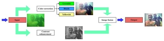
Our goal was to achieve both color correction and contrast enhancement for different underwater scenes. One single color correction method is not suitable for all underwater scenes, while a single enhancement algorithm cannot obtain the effect of image color correction and contrast enhancement at the same time. The flowchart diagram of the whole method is shown in Figure 1. First, this paper divides the underwater images into several categories and adopts different color correction algorithms for different color cast types to achieve adaptive color correction. Then, in order to obtain contrast-enhanced images, this paper uses homomorphic filtering in the frequency domain to enhance high-frequency detail information and reduce low-frequency background noise in images. However, only one of the above methods alone cannot achieve color correction and contrast enhancement images at the same time, so in this paper, we fuse the color-corrected image and the contrast-improved image on the CIE L*a*b* color space.
3.1. Underwater Image Classification
By analyzing a large number of underwater images, we divided the underwater images into four categories: greenish, blueish, yellowish, and colorless bias. The judgment of image color deviation type is to search the best background area of the original underwater image through the Quadtree searching method [21]. The background light is often estimated as the brightest color in an image since the scattering of light by water particles causes a bright color. Avoiding objects that are brighter than the background light may lead to an unsatisfactory selection of background light. We used the variance to determine the best background area. The formula for scoring the best background area is as follows:
where denotes the variance score of the kth region; is the number of pixels in the kth region; denotes the red, green, and blue color channels of the image; represents the mean value of the image in the kth region; denotes the pixel value of the image in the kth region; , , and indicate the red, green, and blue color channel pixel values in the kth region, respectively.
An example to determine underwater image color cast is illustrated in Figure 2. We first divided the underwater image into four equal sub-regions and then calculated the variance of each region. Because the background light is the brightest color in an image, the highest score region is selected as the candidate region. We repeatedly divided the candidate region into four equal sub-regions and recursively looped the above steps until the size of the candidate region was smaller than a set threshold. The threshold was set to the number of pixels in the candidate areas that is less than 1% of the original image pixels [22], which avoided errors in color-cast judgment caused by bright spots or target interference in the underwater image. It is worth noting that this method can be misjudged when the entire image background is originally colored, but in real-world scenarios, this is rarely the case, so this method is still valid in most cases.
Further, the color deviation type of the underwater image is determined based on the mean value of pixels of each channel in the best background area. Firstly, the red, green, and blue channels in the best background area are separated, and their mean pixel values are calculated. Based on which channel has the highest mean value, the type of color deviation in underwater images can be determined. If the mean values of each channel in the best background area are all equal, then there is no color deviation in the underwater image. The color cast processing of the images is discussed in the next subsection.
3.2. Underwater Image Color Correction
In the previous subsection, the underwater image color cast was divided into four categories. The appearances of the images without distortion are similar to the ground scenes, so we only performed the contrast enhancement process. For several other color distortions, we use different color correction methods.
For the correction of the greenish underwater image color, the image histogram is first drawn, then the density of gray values distribution and the cumulative histogram distribution of gray values are calculated from the histogram, the cumulative distribution is taken as positive, and finally normalized.
For bluish underwater images, the color correction is compensated for the red channel. The green channel is usually the lowest attenuated channel in underwater images and has more details relative to the other two channels. Therefore, the green channel is used as the reference channel to compensate for the highest attenuation channel using the grayscale world assumption method [18,23]. After preliminary compensation of the red channel, a greater dynamic range of image pixel gray levels is achieved by applying gain adjustments to all three channels. The red channel compensation formula is given by Equation (6), and the stretching formula for each channel is Equation (7).
where represents the red channel after compensation; , , and denote the red, green, and blue channels of underwater image; , , and are the mean value in each channel of the best background area, respectively; , , and represent the image values of each channel after dynamic adjustment; , , and are the gain coefficient for each color channel; denotes the difference between the maximum gray level and the minimum gray level of each channel, ; , , and indicate the minimum value of each channel after channel compensation. denotes a constant parameter and is set to 1, which is appropriate for subsequent processing.
For the yellowish images, the red channel is used as the reference channel to compensate for the green channel and blue channel; the compensation forms as follows:
where and represent the green channel and blue channel after compensation, respectively; denotes constant parameter and is also set to 1. The other symbols in the compensation equations of the greenish and bluish images have the same meaning as in Equation (6).
3.3. Detail Restoration
In the previous subsection, we proposed a color correction algorithm for different categories of underwater images, and the quality of the images improved significantly after the color correction algorithm, but obtaining a high authenticity appearance of underwater images is not sufficient; the problem of fog still exists in the color-corrected images, causing low contrast and blurriness.
In this work, homomorphic filtering (HF) is employed to enhance image contrast. The reason for using HF is that the HF relies on the illumination–reflection model of the image to divide the image into incident and reflected components. The incident and the reflection component represent low-frequency and high-frequency parts of the image, respectively [24]. The HF not only enhances the high-frequency information of the image but also attenuates the low-frequency information of the image. It enhances the detailed part of the image and diminishes the background noise, thereby obtaining a high-contrast image. Finally, the limiting contrast adaptive histogram equalization (CLAHE) [25] is used to further enhance the brightness and details of the overall image.
The process of HF is to first convert the original underwater RGB image to a grayscale image and then convert the grayscale image to the frequency domain for HF. An image can be expressed as:
where , , and represent incident component, reflected component, and image coordinates, respectively.
The incident and reflected components cannot be directly separated because they are in the form of multiplication, so it is necessary to take the logarithm of both sides of the above equation to obtain Equation (11):
Fourier transform of both sides of Equation (11) is obtained as follows:
It can be simplified as:
A frequency domain function is used to filter both sides of Equation (13) to obtain Equation (14), and the frequency domain function is the transfer function of the homomorphic filter; it is expressed as Equation (15).
where , , and denote high-frequency gain, low-frequency gain and cutoff frequency, respectively. represents the distance from the frequency to the center frequency .
In practice, the parameter values and are responsible for extracting more features from the input image. The selection of is related to the spectral amplitude contrast corresponding to the illumination scene and reflection coefficient, which generally requires several searches for the optimal value. After experiments, we chose , , and to produce a visually pleasing enhanced effect with more details.
After filtering, the Fourier inverse transform is performed, and the spatial image is finally obtained by taking the inverse logarithmic. The process is expressed as follows:
where and are the incident component and reflected component of the image after HF processing, respectively.
Finally, the CLAHE is applied to further enhance the brightness and details of the overall image.
3.4. Image Fusion
To obtain contrast enhancement and color correction simultaneously, we utilized a channel fusion method to fuse the contrast-enhanced image and color-corrected image on the CIE L*a*b* color space. Since the brightness and color channels are separated on the CIE L*a*b* color space, we transformed the contrast-enhanced image and color-corrected image to the CIE L*a*b*color space. The L* channel of contrast-enhanced image has more details of the scene, while the a* channel and the b* channel of the color-corrected image have more accurate color information. Then, we fused the best results of two processing methods while obtaining images with contrast-enhanced color correction, and the fused image is computed as:
where is the final fused image. is the L channel of contrast-enhanced image. and denote the a* channel and the b* channel of the color-corrected image, respectively. is the coefficient of fusion, which is adjusted to change the background color to make the fused image more underwater. represents the image fusion function used to join three arrays into one matrix. Finally, we converted the Lab color space to RGB space. As shown in Figure 3, the color-corrected and contrast-enhanced image was acquired from the previous two subsections, but its processing resulted in haze or no color. The without fusion illustrates that HF, after color correction of RGB color channels, obtains wrong results. The fusion method can obtain color correction and contrast enhancement images at the same time.
4. Results and Evaluation
In this section, we first verify the proposed underwater image processing method. Subjective qualitative evaluation, quantitative evaluation, and application test are implemented. Then, we compare our method with other specialized image restoration/enhancement methods, including MSRCR [26], GDCR [27], IBLA [28], and Two-step [29].
4.1. Validation of Our Method
To validate the effect of contrast enhancement and color correction, we randomly selected four raw images with different color bias types from UIEB [30] and EUVP [31] datasets to demonstrate the verified effect of the proposed method. We classified these images into four categories: greenish images, bluish images, yellowish images, and undistorted images. UIEB is a comprehensive research and analysis of real-world datasets, including 950 real-world underwater images. EUVP contains separate sets of paired and unpaired images of poor and good perceptual quality. All codes were from open-source codes. In experiments, we used the method proposed in the previous section to perform color correction and contrast enhancement on these images.
Figure 4a shows the raw underwater images, which exhibit color distortion or low contrast. For undistorted images, we only enhance their contrast. For the other category of color-cast underwater images, we process it in the following ways: green correction method, blue correction method, and yellow correction method. Figure 4b uses an image enhancement method based on HF, which performs well in terms of clarity. Figure 4c shows the result of color correction, which can be seen to have a realistic appearance but has little effect on the images of detail. Figure 4d shows the results of the fusion of contrast enhancement and color correction on the CIE L*a*b*, which not only removes color deviations but also highlights structural details because it could make full use of the advantages of the two input images of the fusion.
4.2. Comparison with Other Methods
This section compares the methods of MSRCR, GDCP, IBLA, and Two-step. The results are shown in Figure 5, Figure 6 and Figure 7. The histogram distribution of the RGB channels after processing by each algorithm is also plotted.
As can be seen in Figure 5b, Figure 6b and Figure 7b, MSRCR is based on the SSR algorithm to introduce the color recovery factor, but its effect on color correction is very limited and even appears to color shift for bluish images. GDCP has poor color correction results and image contrast results, as depicted in Figure 5c, Figure 6c and Figure 7c. This is due to the attenuation of the red channel in the underwater image, which makes it difficult to obtain accurate depth of the underwater image scene when estimating the underwater image. In Figure 7d, IBLA produces blue artifacts, while in Figure 5d and Figure 6d, it can hardly remove unwanted color casts and has no noticeable effect on contrast enhancement. As shown in Figure 5e and Figure 6e, the Two-step algorithm is effective for color correction of greenish and yellowish images. However, as depicted in Figure 7e, Two-step introduces undesirable reddish distortion in the processing image, and the resulting images have low local contrast and unclear details. Our method achieves good results in processing various categories of color-cast underwater images and improves the contrast and texture of the image, as shown in Figure 5f, Figure 6f and Figure 7f. From the histograms of the RGB color channels, it can also be seen that the RGB color channels of the image processed by our method are the closest, indicating the minimum difference and the best color correction for the image.
Figure 8 presents the results of these methods on a wide range of underwater images from the UIEB [30] and the UCCS [32] datasets. UCCS contains three subsets: blue, blue-green, and green subsets. We selected multiple images of each type for a comprehensive comparison. The method of GDCP only slightly improves the images. The IBLA has little effect on the images and produces blue artifacts for some yellowish images. The MSRCR corrects the color to a certain extent, but the specific details of the image are not well revealed. The Two-step has good performance, but it does not dehaze and has little effect on the images with a green appearance. However, ours can eliminate the color cast and excels well in terms of clarity.
To quantitatively evaluate the performance of the processing methods of underwater images in Figure 8, we present the UCIQE [33], UIQM [34], PCQI [35], and EME [36] scores of different methods in Table 1 and Table 2. UCIQE is a linear combination of chroma, saturation, and contrast to quantitatively assess the blurring, non-uniform chromatic aberration, and contrast of underwater images. The larger the value of UCIQE, the better the image in terms of color balance, sharpness, and contrast. UIQM is a comprehensive image evaluation criterion for underwater image degradation mechanisms, with higher values representing images with higher contrast, sharpness, and color balance. PCQI calculates the average intensity, information intensity, and signal structure in each image block and evaluates the distortion of the image in these three perspectives, with larger values representing better image contrast. The EME divides the image into small areas, calculates the ratio of the maximum and minimum grayscale values in each area, and then calculates the average contrast of all areas as the image quality of the global image, and the higher the EME value, the better the image quality.
From the quantitative evaluation values in Table 1 and Table 2, the proposed method obtains the highest scores for most evaluation metrics. For better evaluation, we plotted the distribution of the mean values of the four evaluation indicators for different processing methods; as depicted in Figure 9, the average value of our method is the highest, and the distribution curve of the average value is at the top layer, indicating that our method is superior to the other four image processing methods. Comprehensively, the results of subjective evaluation and objective evaluation demonstrate that our method has higher contrast, more detailed features, and a more realistic appearance.
4.3. Application Tests
To further show the effectiveness of our method, we built a custom system for underwater imaging, which can be used at a depth of 100 m. The system is shown in Figure 10a. The system capture device uses the integrated movement of Hikvision (DS-2ZMN0409S), which allows for installation in a smaller sealed compartment. The internal automatic white balance function of the capture device is turned off. The system housing is manufactured by 316L stainless steel and is commercially available.
We performed experiments in a real pool and placed a wooden stick, a plastic shell, and fishing nets in the water as an underwater scene. The size of the test pool is 15 m × 8 m × 6 m, as depicted in Figure 10b. We used a homemade underwater camera to capture images. Six different object distances were set in experiments, i.e., 1 m, 2 m, 3 m, 4 m, 5 m, and 6 m. The depth of equipment is approximately 1–1.5 m, and the camera was placed in the center of the pool. The experimental pool was indoors, and the experiment was conducted during the daytime, using only indoor fluorescent lighting sources with an intensity of approximately 300 Lux, with no additional light sources added to the pool. In practical use, if the detection water is deep or the water quality has high turbidity, additional light sources can be added according to actual needs, or even polarized light sources can be added to suppress scattered light interference.
The real experimental underwater images are shown in the left column of Figure 11; the distance increases from top to bottom. It can be seen that the appearance of the images is greenish, and as the distance increases, the images become blurry due to the scattering and absorption of water. Figure 11f shows the restoration results of our method under different distance conditions, while these results are compared with other methods and assessed by image quality evaluation metric. As can be observed, the approaches of MSRCR, GDCP, and IBLA perform poorly in processing images of different distances. Two-step can eliminate the color deviation to a certain extent, but it produces red artifacts. However, the image color correction by our method is visually pleasing. Meanwhile, the contrast and details are well enhanced. Figure 11g,h presents enlarged views of the details in a red dashed rectangle. We can easily see the fishing net from the enlarged image, and as the distance increases, our method remains effective, which demonstrates the good generalization performance of our method. Table 3 gives the average evaluation scores of these methods applied to different distances of images in terms of UCIQE, UIQM, PCQI, and EME. From the results, our method obtains the two highest scores and a suboptimal score in the four evaluation criteria. In summary, our proposed method has an excellent appearance and the most quantitative evaluation values.
In addition, because the color bias of the images is related to the water quality, the acquisition of different color deviation images requires the addition of different substances to the water. The pool (15 m × 8 m × 6 m) in this experiment is large, and a large amount of water needs to be replaced after adding substances to the water, so only green images were acquired. In the future, we will capture other colors of water-quality images when there are suitable occasions.
5. Conclusions
In this paper, we introduce an effective underwater image processing method capable of simultaneously enhancing contrast and rectifying color casts. The proposed approach comprises several key steps. Initially, raw underwater images are classified according to the variance of the optimal background region. Subsequently, a color correction step is applied in accordance with the identified color bias, resulting in a color-neutral underwater image. Then, the original underwater image undergoes homomorphic filtering; this procedure accentuates high-frequency information while mitigating low-frequency elements, thereby yielding a high-contrast image. The final step involves the fusion of the contrast-amplified grayscale image and the color-corrected counterpart within the CIE L*a*b* color space, culminating in an enhanced underwater image characterized by improved contrast and color fidelity.
Our proposed method is systematically compared against alternative image restoration/enhancement techniques. Qualitative assessments highlight the method’s ability to render images with a closer approximation to real colors. Quantitative analyses underscore our method’s superior performance across all four objective evaluations. To empirically validate the practical effectiveness of our underwater image processing approach, an experimental setup was constructed. Multiple distance-based experiments were conducted to ascertain the method’s efficacy. It is important to acknowledge that while our method excels at enhancing contrast and correcting color in underwater images, it encounters challenges when dealing with deep, severely turbid underwater environments characterized by low light conditions. Future research will be dedicated to addressing this particularly demanding scenario.
Author Contributions
Conceptualization, W.Z., X.L. (Xiaobo Li) and H.H.; methodology, W.Z., S.X., and X.L. (Xiaobo Li); software, W.Z. and S.X.; validation, S.X., Y.Y., W.Z. and X.L. (Xujin Li); formal analysis, W.Z. and X.L. (Xujin Li); investigation, W.Z. and X.L. (Xiaobo Li); resources, X.L. (Xiaobo Li) and H.H.; data curation, W.Z. and S.X.; writing—original draft preparation, W.Z.; writing—review and editing, W.Z. and X.L. (Xiaobo Li); visualization, W.Z. and X.L. (Xiaobo Li); supervision, H.H.; project administration, H.H., D.X. and T.L.; funding acquisition, H.H. All authors have read and agreed to the published version of the manuscript.
Funding
This research was funded by the National Natural Science Foundation of China (62075161, 62205243) and the Key Laboratory of Equipment and Informatization in Environment Controlled Agriculture, Ministry of Agriculture and Rural Affairs (2011NYZD2201).
Data Availability Statement
Not applicable.
Acknowledgments
The authors would like to thank all anonymous reviewers for their helpful comments and suggestions.
Conflicts of Interest
The authors declare no conflict of interest.
References
- Lin, Y.H.; Yu, C.M.; Wu, C.Y. Towards the Design and Implementation of an Image-Based Navigation System of an Autonomous Underwater Vehicle Combining a Color Recognition Technique and a Fuzzy Logic Controller. Sensors 2021, 21, 4053. [Google Scholar] [CrossRef] [PubMed]
- Chen, L.; Jiang, Z.; Tong, L.; Liu, Z.; Zhao, A.; Zhang, Q.; Dong, J.; Zhou, H. Perceptual Underwater Image Enhancement with Deep Learning and Physical Priors. IEEE Trans. Circuits Syst. Video Technol. 2021, 31, 3078–3092. [Google Scholar] [CrossRef]
- Kahanov, Y.; Royal, J.G. Analysis of hull remains of the Dor D Vessel, Tantura Lagoon, Israel. Int. J. Naut. Archaeol. 2001, 30, 257–265. [Google Scholar] [CrossRef]
- Zhang, W.; Dong, L.; Zhang, T.; Xu, W. Enhancing underwater image via color correction and Bi-interval contrast enhancement. Signal Process. Image Commun. 2021, 90, 116030. [Google Scholar] [CrossRef]
- Schechner, Y.Y.; Karpel, N. Recovery of underwater visibility and structure by polarization analysis. IEEE J. Ocean. Eng. 2005, 30, 570–587. [Google Scholar] [CrossRef]
- Hu, H.; Qi, P.; Li, X.; Cheng, Z.; Liu, T. Underwater imaging enhancement based on a polarization filter and histogram attenuation prior. J. Phys. D Appl. Phys. 2021, 54, 175102. [Google Scholar] [CrossRef]
- Li, X.; Han, Y.; Wang, H.; Liu, T.; Chen, S.-C.; Hu, H. Polarimetric Imaging Through Scattering Media: A Review. Front. Phys. 2022, 10, 815296. [Google Scholar] [CrossRef]
- Li, X.; Zhang, L.; Qi, P.; Zhu, Z.; Xu, J.; Liu, T.; Zhai, J.; Hu, H. Are Indices of Polarimetric Purity Excellent Metrics for Object Identification in Scattering Media? Remote Sens. 2022, 14, 4148. [Google Scholar] [CrossRef]
- Li, X.; Xu, J.; Zhang, L.; Hu, H.; Chen, S.-C. Underwater image restoration via Stokes decomposition. Opt. Lett. 2022, 47, 2854–2857. [Google Scholar] [CrossRef]
- Li, X.; Hu, H.; Zhao, L.; Wang, H.; Yu, Y.; Wu, L.; Liu, T. Polarimetric image recovery method combining histogram stretching for underwater imaging. Sci. Rep. 2018, 8, 12430. [Google Scholar] [CrossRef]
- Azmi, K.Z.M.; Ghani, A.S.A.; Yusof, Z.M.; Ibrahim, Z. Natural-based underwater image color enhancement through fusion of swarm-intelligence algorithm. Appl. Soft Comput. 2019, 85, 105810. [Google Scholar] [CrossRef]
- Zhang, W.D.; Dong, L.L.; Pan, X.P.; Zhou, J.C.; Qin, L.; Xu, W.H. Single Image Defogging Based on Multi-Channel Convolution MSRCR. IEEE Access 2019, 7, 72492–72504. [Google Scholar] [CrossRef]
- Sethi, R.; Indu, S. Fusion of Underwater Image Enhancement and Restoration. Int. J. Pattern Recognit. Artif. Intell. 2020, 34, 2054007. [Google Scholar] [CrossRef]
- Xu, L.; Ren, J.S.J.; Liu, C.; Jia, J. Deep Convolutional Neural Network for Image Deconvolution. In Proceedings of the International Conference on Neural Information Processing Systems, Montreal, QC, Canada, 8–13 December 2014; pp. 1790–1798. [Google Scholar]
- Li, J.; Skinner, K.A.; Eustice, R.M.; Johnson-Roberson, M. WaterGAN: Unsupervised Generative Network to Enable Real-Time Color Correction of Monocular Underwater Images. IEEE Rob. Autom. Lett. 2018, 3, 387–394. [Google Scholar] [CrossRef]
- Hu, H.; Yang, S.; Li, X.; Cheng, Z.; Liu, T.; Zhai, J. Polarized image super-resolution via a deep convolutional neural network. Opt. Express 2023, 31, 8535–8547. [Google Scholar] [CrossRef]
- Li, X.; Yan, L.; Qi, P.; Zhang, L.; Goudail, F.; Liu, T.; Zhai, J.; Hu, H. Polarimetric Imaging via Deep Learning: A Review. Remote Sens. 2023, 15, 1540. [Google Scholar] [CrossRef]
- Ancuti, C.O.; Ancuti, C.; De Vleeschouwer, C.; Bekaert, P. Color Balance and Fusion for Underwater Image Enhancement. IEEE Trans. Image Process. 2018, 27, 379–393. [Google Scholar] [CrossRef]
- McGlamery, B. A Computer Model For Underwater Camera Systems. Proc. SPIE 1979, 208, 221–231. [Google Scholar] [CrossRef]
- Jaffe, J.S. Computer modeling and the design of optimal underwater imaging systems. IEEE J. Ocean. Eng. 1990, 15, 101–111. [Google Scholar] [CrossRef]
- Gong, M.L.; Yang, Y.H. Quadtree-based genetic algorithm and its applications to computer vision. Pattern Recogn. 2004, 37, 1723–1733. [Google Scholar] [CrossRef]
- Hou, G.J.; Zhao, X.; Pan, Z.K.; Yang, H.; Tan, L.; Li, J.M. Benchmarking Underwater Image Enhancement and Restoration, and Beyond. IEEE Access 2020, 8, 122078–122091. [Google Scholar] [CrossRef]
- Li, Y.M.; Zhu, C.L.; Peng, J.X.; Bian, L.H. Fusion-based underwater image enhancement with category-specific color correction and dehazing. Opt. Express 2022, 30, 33826–33841. [Google Scholar] [CrossRef] [PubMed]
- Zhang, C.; Liu, W.; Xing, W. Color image enhancement based on local spatial homomorphic filtering and gradient domain variance guided image filtering. J. Electron. Imaging 2018, 27, 063026. [Google Scholar] [CrossRef]
- Hitam, M.S.; Yussof, W.; Awalludin, E.A.; Bachok, Z.; IEEE. Mixture Contrast Limited Adaptive Histogram Equalization for Underwater Image Enhancement. In Proceedings of the International Conference on Computer Applications Technology, Sousse, Tunisia, 20–22 January 2013; pp. 1–5. [Google Scholar]
- Jobson, D.J.; Rahman, Z.; Woodell, G.A. A multiscale retinex for bridging the gap between color images and the human observation of scenes. IEEE Trans. Image Process. 1997, 6, 965–976. [Google Scholar] [CrossRef] [PubMed]
- Peng, Y.T.; Cao, K.M.; Cosman, P.C. Generalization of the Dark Channel Prior for Single Image Restoration. IEEE Trans. Image Process. 2018, 27, 2856–2868. [Google Scholar] [CrossRef] [PubMed]
- Peng, Y.T.; Cosman, P.C. Underwater Image Restoration Based on Image Blurriness and Light. IEEE Trans. Image Process. 2017, 26, 1579–1594. [Google Scholar] [CrossRef]
- Fu, X.Y.; Fan, Z.W.; Ling, M.; Huang, Y.; Ding, X.H. Two-step approach for single underwater image enhancement. In Proceedings of the International Symposium on Intelligent Signal Processing and Communication Systems (ISPACS 2017), Xianmen, China, 6–9 November 2017; pp. 789–794. [Google Scholar]
- Li, C.; Guo, C.; Ren, W.; Cong, R.; Hou, J.; Kwong, S.; Tao, D. An Underwater Image Enhancement Benchmark Dataset and Beyond. IEEE Trans. Image Process. 2020, 29, 4376–4389. [Google Scholar] [CrossRef]
- Islam, M.J.; Xia, Y.Y.; Sattar, J. Fast Underwater Image Enhancement for Improved Visual Perception. IEEE Rob. Autom. Lett. 2020, 5, 3227–3234. [Google Scholar] [CrossRef]
- Liu, R.S.; Fan, X.; Zhu, M.; Hou, M.J.; Luo, Z.X. Real-World Underwater Enhancement: Challenges, Benchmarks, and Solutions Under Natural Light. IEEE Trans. Circuits Syst. Video Technol. 2020, 30, 4861–4875. [Google Scholar] [CrossRef]
- Yang, M.; Sowmya, A. An Underwater Color Image Quality Evaluation Metric. IEEE Trans. Image Process. 2015, 24, 6062–6071. [Google Scholar] [CrossRef]
- Panetta, K.; Gao, C.; Agaian, S. Human-Visual-System-Inspired Underwater Image Quality Measures. IEEE J. Ocean. Eng. 2016, 41, 541–551. [Google Scholar] [CrossRef]
- Wang, S.Q.; Ma, K.D.; Yeganeh, H.; Wang, Z.; Lin, W.S. A Patch-Structure Representation Method for Quality Assessment of Contrast Changed Images. IEEE Signal Process Lett. 2015, 22, 2387–2390. [Google Scholar] [CrossRef]
- Agaian, S.S.; Panetta, K.; Grigoryan, A.M. Transform-based image enhancement algorithms with performance measure. IEEE Trans. Image Process. 2001, 10, 367–382. [Google Scholar] [CrossRef] [PubMed]
Figure 1.
Flowchart of the proposed method.

Figure 2.
An illustration to search for the best background area (The red lines indicate the region of each division and the circle denotes the area of the final selection).
Figure 2.
An illustration to search for the best background area (The red lines indicate the region of each division and the circle denotes the area of the final selection).

Figure 3.
The ablation experiment compares different fusion and without-fusion underwater images.

Figure 4.
The processing results of different color-cast images.

Figure 5.
Greenish image processing result and corresponding tricolor histograms: (a) raw images and corresponding tricolor histograms; (b) result using the method of MSRCR and corresponding tricolor histograms; (c) result using the method of GDCP and corresponding tricolor histograms; (d) result using the method of IBLA and corresponding tricolor histograms; (e) result using the method of Two-step and corresponding tricolor histograms; (f) result using our method and corresponding tricolor histograms.

Figure 6.
Bluish image processing result and corresponding tricolor histograms: (a) raw images and corresponding tricolor histograms; (b) result using the method of MSRCR and corresponding tricolor histograms; (c) result using the method of GDCP and corresponding tricolor histograms; (d) result using the method of IBLA and corresponding tricolor histograms; (e) result using the method of Two-step and corresponding tricolor histograms; (f) result using our method and corresponding tricolor histograms.

Figure 7.
Yellowish image processing result and corresponding tricolor histograms: (a) raw images and corresponding tricolor histograms; (b) result using the method of MSRCR and corresponding tricolor histograms; (c) result using the method of GDCP and corresponding tricolor histograms; (d) result using the method of IBLA and corresponding tricolor histograms; (e) result using the method of Two-step and corresponding tricolor histograms; (f) result using our method and corresponding tricolor histograms.

Figure 8.
Visual comparison: (a–n) different types of underwater images from UIEB dataset and UCCS dataset.
Figure 8.
Visual comparison: (a–n) different types of underwater images from UIEB dataset and UCCS dataset.

Figure 9.
Distribution of evaluation average values for different image processing methods.

Figure 10.
(a) Underwater cameras; (b) test pool.

Figure 11.
Experimental results under different distances. Distance increases from top to bottom: (a) raw images; (b) MSRCR; (c) GDCP; (d) IBLA; (e) Two-step; (f) ours; (g,h) the enlarged images in a red dashed rectangle.
Figure 11.
Experimental results under different distances. Distance increases from top to bottom: (a) raw images; (b) MSRCR; (c) GDCP; (d) IBLA; (e) Two-step; (f) ours; (g,h) the enlarged images in a red dashed rectangle.


Table 1.
UCIQE and UIQM values of different methods in Figure 8.
Table 1.
UCIQE and UIQM values of different methods in Figure 8.
| Methods | MSRCR | GDCP | IBLA | Two-Step | Ours | |||||
|---|---|---|---|---|---|---|---|---|---|---|
| UCIQE | UIQM | UCIQE | UIQM | UCIQE | UIQM | UCIQE | UIQM | UCIQE | UIQM | |
| (a) | 0.534 | 3.548 | 0.360 | −1.993 | 0.374 | −0.136 | 0.467 | 3.472 | 0.596 | 5.323 |
| (b) | 0.583 | 3.012 | 0.537 | 2.983 | 0.518 | 1.432 | 0.552 | 3.299 | 0.648 | 4.693 |
| (c) | 0.500 | 4.062 | 0.373 | 1.460 | 0.427 | 2.088 | 0.458 | 4.408 | 0.585 | 4.972 |
| (d) | 0.510 | 5.414 | 0.368 | −0.367 | 0.411 | −0.221 | 0.420 | 3.472 | 0.582 | 5.021 |
| (e) | 0.521 | 2.329 | 0.371 | −1.124 | 0.505 | 0.643 | 0.608 | 4.274 | 0.383 | 4.448 |
| (f) | 0.488 | 3.165 | 0.628 | 3.993 | 0.542 | 1.316 | 0.566 | 5.192 | 0.547 | 5.412 |
| (g) | 0.458 | 2.749 | 0.517 | 0.565 | 0.555 | 2.172 | 0.584 | 5.318 | 0.542 | 5.236 |
| (h) | 0.506 | 3.236 | 0.672 | 4.635 | 0.522 | 1.651 | 0.598 | 4.936 | 0.565 | 4.966 |
| (i) | 0.556 | 2.432 | 0.558 | 0.749 | 0.599 | 1.880 | 0.612 | 4.939 | 0.569 | 4.968 |
| (j) | 0.560 | 2.862 | 0.538 | 0.987 | 0.503 | 2.198 | 0.581 | 4.198 | 0.618 | 4.350 |
| (k) | 0.477 | 2.607 | 0.546 | 3.362 | 0.492 | 4.218 | 0.479 | 4.018 | 0.526 | 4.451 |
| (l) | 0.534 | 1.649 | 0.491 | 1.718 | 0.632 | 1.082 | 0.514 | 1.674 | 0.519 | 2.084 |
| (m) | 0.502 | 2.793 | 0.659 | 4.862 | 0.691 | 5.021 | 0.587 | 4.078 | 0.570 | 3.854 |
| (n) | 0.523 | 3.385 | 0.516 | 3.586 | 0.615 | 2.628 | 0.521 | 4.031 | 0.577 | 4.340 |
The bold highlights the best indicator results.
Table 2.
PCQI and EME values of different methods in Figure 8.
Table 2.
PCQI and EME values of different methods in Figure 8.
| Methods | MSRCR | GDCP | IBLA | Two-Step | Ours | |||||
|---|---|---|---|---|---|---|---|---|---|---|
| PCQI | EME | PCQI | EME | PCQI | EME | PCQI | EME | PCQI | EME | |
| (a) | 1.305 | 21.145 | 1.042 | 12.341 | 1.022 | 4.030 | 1.276 | 14.710 | 1.327 | 21.285 |
| (b) | 1.017 | 14.258 | 0.897 | 7.824 | 1.067 | 7.665 | 1.189 | 10.742 | 1.259 | 10.272 |
| (c) | 1.130 | 3.464 | 0.962 | 2.732 | 1.105 | 4.961 | 1.162 | 4.954 | 1.231 | 9.261 |
| (d) | 1.261 | 3.466 | 1.002 | 7.237 | 1.124 | 11.647 | 1.170 | 6.848 | 1.308 | 14.157 |
| (e) | 0.700 | 1.706 | 0.623 | 3.555 | 1.082 | 8.197 | 0.853 | 4.909 | 0.911 | 7.321 |
| (f) | 0.850 | 5.379 | 1.182 | 15.208 | 1.127 | 11.646 | 1.337 | 16.101 | 1.397 | 16.802 |
| (g) | 0.655 | 8.226 | 0.853 | 16.317 | 1.115 | 18.587 | 1.330 | 23.183 | 1.343 | 22.967 |
| (h) | 0.882 | 5.833 | 1.17 | 19.039 | 1.099 | 15.552 | 1.300 | 16.496 | 1.352 | 18.453 |
| (i) | 0.600 | 10.277 | 0.857 | 19.848 | 1.049 | 10.764 | 1.257 | 24.038 | 1.278 | 26.479 |
| (j) | 0.943 | 5.322 | 0.834 | 5.051 | 1.122 | 11.464 | 1.096 | 7.748 | 1.204 | 17.517 |
| (k) | 0.958 | 2.035 | 0.983 | 4.478 | 0.979 | 1.885 | 1.113 | 4.431 | 1.267 | 6.847 |
| (l) | 0.865 | 1.144 | 0.796 | 1.225 | 1.035 | 2.340 | 0.965 | 1.769 | 1.053 | 3.638 |
| (m) | 0.949 | 1.714 | 1.060 | 2.946 | 1.011 | 4.395 | 1.066 | 4.026 | 1.205 | 6.046 |
| (n) | 0.999 | 2.080 | 0.929 | 2.084 | 0.722 | 2.887 | 1.149 | 3.733 | 1.264 | 7.640 |
The bold highlights the best indicator results.
Table 3.
Average quantitative results of evaluation in Figure 11.
Table 3.
Average quantitative results of evaluation in Figure 11.
| Methods | UCIQE | UIQM | PCQI | EME |
|---|---|---|---|---|
| MSRCR | 0.294 | −1.011 | 0.686 | 0.745 |
| GDCP | 0.397 | −2.097 | 0.875 | 2.163 |
| IBLA | 0.449 | −0.991 | 1.030 | 4.194 |
| Two-step | 0.482 | 1.884 | 1.052 | 2.759 |
| Ours | 0.502 | 1.984 | 1.003 | 3.874 |
The bold is highlights the best indicator results.
Disclaimer/Publisher’s Note: The statements, opinions and data contained in all publications are solely those of the individual author(s) and contributor(s) and not of MDPI and/or the editor(s). MDPI and/or the editor(s) disclaim responsibility for any injury to people or property resulting from any ideas, methods, instructions or products referred to in the content. |
© 2023 by the authors. Licensee MDPI, Basel, Switzerland. This article is an open access article distributed under the terms and conditions of the Creative Commons Attribution (CC BY) license (https://creativecommons.org/licenses/by/4.0/).
Share and Cite
MDPI and ACS Style
Zhang, W.; Li, X.; Xu, S.; Li, X.; Yang, Y.; Xu, D.; Liu, T.; Hu, H. Underwater Image Restoration via Adaptive Color Correction and Contrast Enhancement Fusion. Remote Sens. 2023, 15, 4699. https://doi.org/10.3390/rs15194699
AMA Style
Zhang W, Li X, Xu S, Li X, Yang Y, Xu D, Liu T, Hu H. Underwater Image Restoration via Adaptive Color Correction and Contrast Enhancement Fusion. Remote Sensing. 2023; 15(19):4699. https://doi.org/10.3390/rs15194699
Chicago/Turabian StyleZhang, Weihong, Xiaobo Li, Shuping Xu, Xujin Li, Yiguang Yang, Degang Xu, Tiegen Liu, and Haofeng Hu. 2023. "Underwater Image Restoration via Adaptive Color Correction and Contrast Enhancement Fusion" Remote Sensing 15, no. 19: 4699. https://doi.org/10.3390/rs15194699
Note that from the first issue of 2016, this journal uses article numbers instead of page numbers. See further details here.