
Impact of Deep Convolutional Neural Network Structure on Photovoltaic Array Extraction from High Spatial Resolution Remote Sensing Images


1
State Key Laboratory of Resources and Environmental Information System, Institute of Geographic Sciences and Natural Resources Research, Chinese Academy of Sciences, Beijing 100101, China
2
University of Chinese Academy of Sciences, Beijing 100049, China
3
Jiangsu Center for Collaborative Innovation in Geographical Information Resource Development and Application, Nanjing Normal University, No. 1, Wenyuan Road, Qixia, Nanjing 210023, China
*
Author to whom correspondence should be addressed.
Remote Sens. 2023, 15(18), 4554; https://doi.org/10.3390/rs15184554
Submission received: 11 August 2023
/
Revised: 5 September 2023
/
Accepted: 13 September 2023
/
Published: 15 September 2023
(This article belongs to the Section AI Remote Sensing)
Abstract
:Accurate information on the location, shape, and size of photovoltaic (PV) arrays is essential for optimal power system planning and energy system development. In this study, we explore the potential of deep convolutional neural networks (DCNNs) for extracting PV arrays from high spatial resolution remote sensing (HSRRS) images. While previous research has mainly focused on the application of DCNNs, little attention has been paid to investigating the influence of different DCNN structures on the accuracy of PV array extraction. To address this gap, we compare the performance of seven popular DCNNs—AlexNet, VGG16, ResNet50, ResNeXt50, Xception, DenseNet121, and EfficientNetB6—based on a PV array dataset containing 2072 images of 1024 × 1024 size. We evaluate their intersection over union (IoU) values and highlight four DCNNs (EfficientNetB6, Xception, ResNeXt50, and VGG16) that consistently achieve IoU values above 94%. Furthermore, through analyzing the difference in the structure and features of these four DCNNs, we identify structural factors that contribute to the extraction of low-level spatial features (LFs) and high-level semantic features (HFs) of PV arrays. We find that the first feature extraction block without downsampling enhances the LFs’ extraction capability of the DCNNs, resulting in an increase in IoU values of approximately 0.25%. In addition, the use of separable convolution and attention mechanisms plays a crucial role in improving the HFs’ extraction, resulting in a 0.7% and 0.4% increase in IoU values, respectively. Overall, our study provides valuable insights into the impact of DCNN structures on the extraction of PV arrays from HSRRS images. These findings have significant implications for the selection of appropriate DCNNs and the design of robust DCNNs tailored for the accurate and efficient extraction of PV arrays.
1. Introduction
The utilization of fossil fuel-based energy sources poses various challenges such as resource depletion, carbon emissions, and environmental degradation [1]. In order to achieve sustainable development and mitigate climate change, many countries are actively promoting the adoption of clean energy sources. Among these alternatives, solar energy is of great interest due to its significant environmental benefits [2]. Owing to the declining costs of solar photovoltaic (PV) modules and government support, solar PV has experienced rapid growth in recent decades [3], reaching a global installed capacity of approximately 1062 GW by the end of 2022 [4]. In this context, accurate information on the location, shape, and size of PV arrays is meaningful and essential for optimizing power system planning [5], predicting the generation potential [6], and facilitating the overall development of energy systems [7].
The PV array extraction from remote sensing images is an effective way to obtain this type of information [8,9]. With the advancement of sensor technology, high spatial resolution remote sensing (HSRRS) images have become a preferred choice for achieving high-precision PV array extraction [10,11]. This type of extraction requires the effective separation of the image into PV and non-PV arrays, which can be accomplished by three main approaches: digital image processing methods [12,13], machine learning classification methods [14,15], and deep learning segmentation methods [16,17].
Digital image processing methods use PV feature priors, edge segmentation, or template matching techniques to extract PV arrays. For instance, Grimaccia et al. [13] utilized a color space conversion from RGB to HSV and set thresholds based on PV color feature priors to extract PV arrays. Carletti et al. [12] combined the Canny algorithm and the Hough transform to detect the straight lines on which the edges of the PV panels are located. The edges of each PV panel were then extracted from these straight lines according to the shape priors of the PV panel. Although these methods can accurately extract PV panels from a single scene containing only PV arrays by using the color and shape of the PV panels as priors, their accuracy is limited in complex scenes due to the interference from analogous objects such as vegetable patches and sheds [18].
Machine learning classification methods typically employ manually selected classification features to classify image pixels for PV array extraction. For example, Zhang et al. [19] selected texture features calculated from SAR images, five raw spectral features, and three normalized indicators as classification features for a random forest classifier to automatically extract PV arrays. Chen et al. [20] constructed PV extraction indices based on a thorough comparative analysis of the spectral features of PV arrays and other objects. These indices are then combined with the original spectral features and terrain features as classification features for XGBoost [21] to extract PV arrays. Since the better classification features were manually selected, the machine learning classification methods can achieve better PV array extraction with a small amount of training data. However, these features are influenced by the lighting conditions, photographic angle, and geographical variations, making such methods unsuitable for extracting PV arrays in large regions with complex backgrounds [22].
Deep learning segmentation methods use semantic segmentation models to extract PV arrays from images. Specifically, this kind of model first uses deep convolutional neural networks (DCNNs), known as the backbone of the models, to extract both low-level spatial features (LFs) and the high-level semantic features (HFs) of PV arrays. These features are then combined and upsampled using specific semantic segmentation architectures, such as DeeplabV3_plus [23], for mapping back to the spatial scale of the original image. Semantic classification is then applied to each pixel to identify PV arrays. For example, Sizkouhi et al. [18] combined a VGG16 DCNN [24] with a Mask R-CNN architecture [25] to automatically extract PV array boundaries. Wu et al. [16] used a ResNet DCNN [26] with pre-trained weights to extract multilevel features and combined it with the U-Net architecture [27] to extract distributed PV arrays. Jie et al. [22] integrated an EfficientNet DCNN [28] and U-Net architecture for PV array extraction, while designing a gated fusion module to improve the extraction accuracy for small-scale PV arrays.
Compared to the first two methods, deep learning segmentation methods have demonstrated a superior performance in PV array extraction. This is mainly due to the advanced feature extraction capabilities of DCNNs [29]. Different DCNN structures have varying feature extraction capabilities, resulting in diverse object extraction results [30]. However, for extracting PV arrays from HSRRS images, previous research has mainly focused on the application of DCNNs, and little attention has been paid to investigate the influence of DCNN structures on PV array feature extraction.
The primary motivation of this study is to explore the structural factors that favor the extraction of PV array features. To this end, we first perform a comprehensive comparison of seven typical DCNNs—AlexNet [31], Xception [32], ResNet50, VGG16, DenseNet121 [33], ResNeXt50 [34], and EfficientNetB6—for extracting PV arrays from HSRRS images. Then, by analyzing the features and structural differences of the better performing DCNNs, we identify the structural factors conducive to the extraction of different levels of PV array features. To the best of our knowledge, exploring the beneficial structural factors for PV array feature extraction through the comparison of different DCNNs in extracting PV arrays from HSRRS images has been lacking so far.
The remainder of the paper is organized as follows: the dataset and its pre-processing are detailed in Section 2; Section 3 describes the experimental methods; Section 4 provides a detailed comparison of different DCNNs under the DeeplabV3_plus architecture; Section 5 analyzes the structural factor in favor of the PV array feature extraction; Section 6 presents a discussion. Section 7 summarizes the conclusions.
2. Dataset
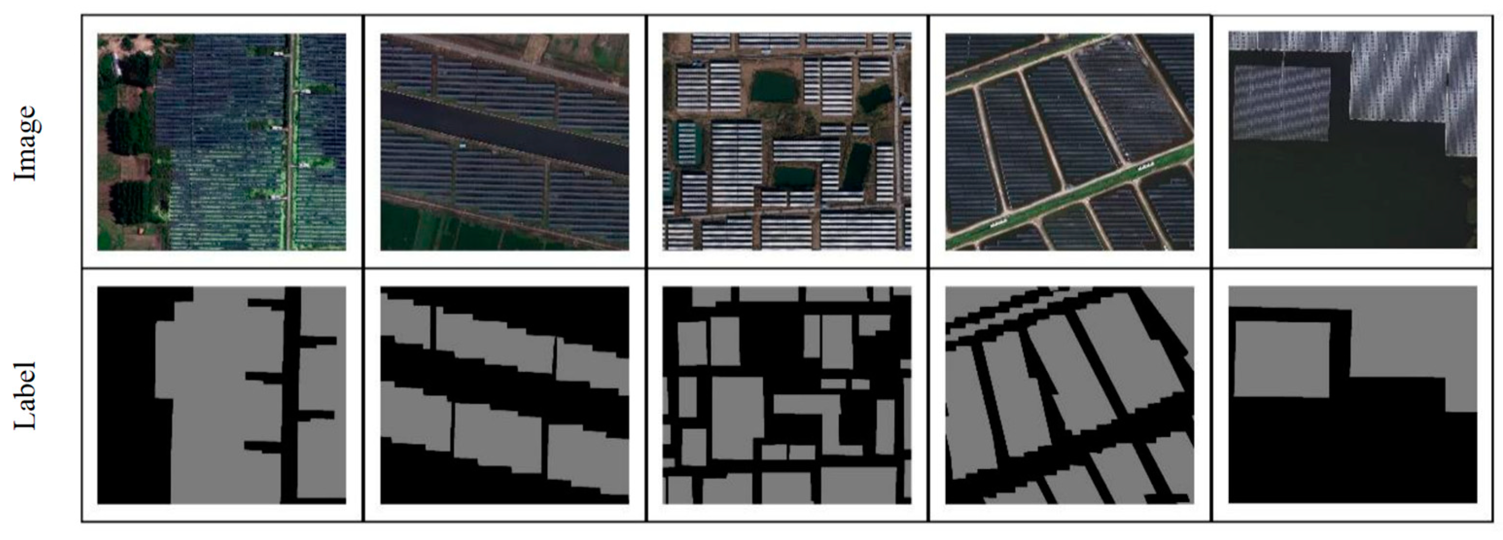
In this study, we use a PV array sample dataset with an image spatial resolution of 0.3 m. This dataset is obtained from the multi-resolution PV dataset published by Jiang et al. [35]. The images are acquired through aerial photography conducted over Jiangsu Province, China. Subsequently, a series of image processing procedures are applied to enhance their quality, such as cloud cover removal, noise reduction, geometric correction, orthogonal correction, and histogram equalization. PV array labels are obtained by manual annotation. The dataset consists of 2072 PV array samples, each with a size of 1024 × 1024—comprising both the image itself and its corresponding label. Figure 1 shows some PV array samples contained within the dataset.
To perform the experiments, a pre-processing operation is applied to the dataset, which includes the following steps: (1) mismatches between images and labels are manually corrected to ensure the accuracy of all samples; (2) each image subtracts its own mean, and divided by its standard deviation to allow for faster model convergence during training; (3) labels are binarized so that each pixel has a value of either 1 (for PV array pixels) or 0 (for non-PV array pixels); (4) each sample is cropped into four 512 × 512-sized samples; (4) 80% of the samples are randomly selected as the training set (among which 20% were used for validation) and 20% as the test set; (5) for data augmentation, various transformations such as flipping, rotation, brightness and contrast adjustments and Gaussian blurring are applied to the training set samples.
3. Methodology
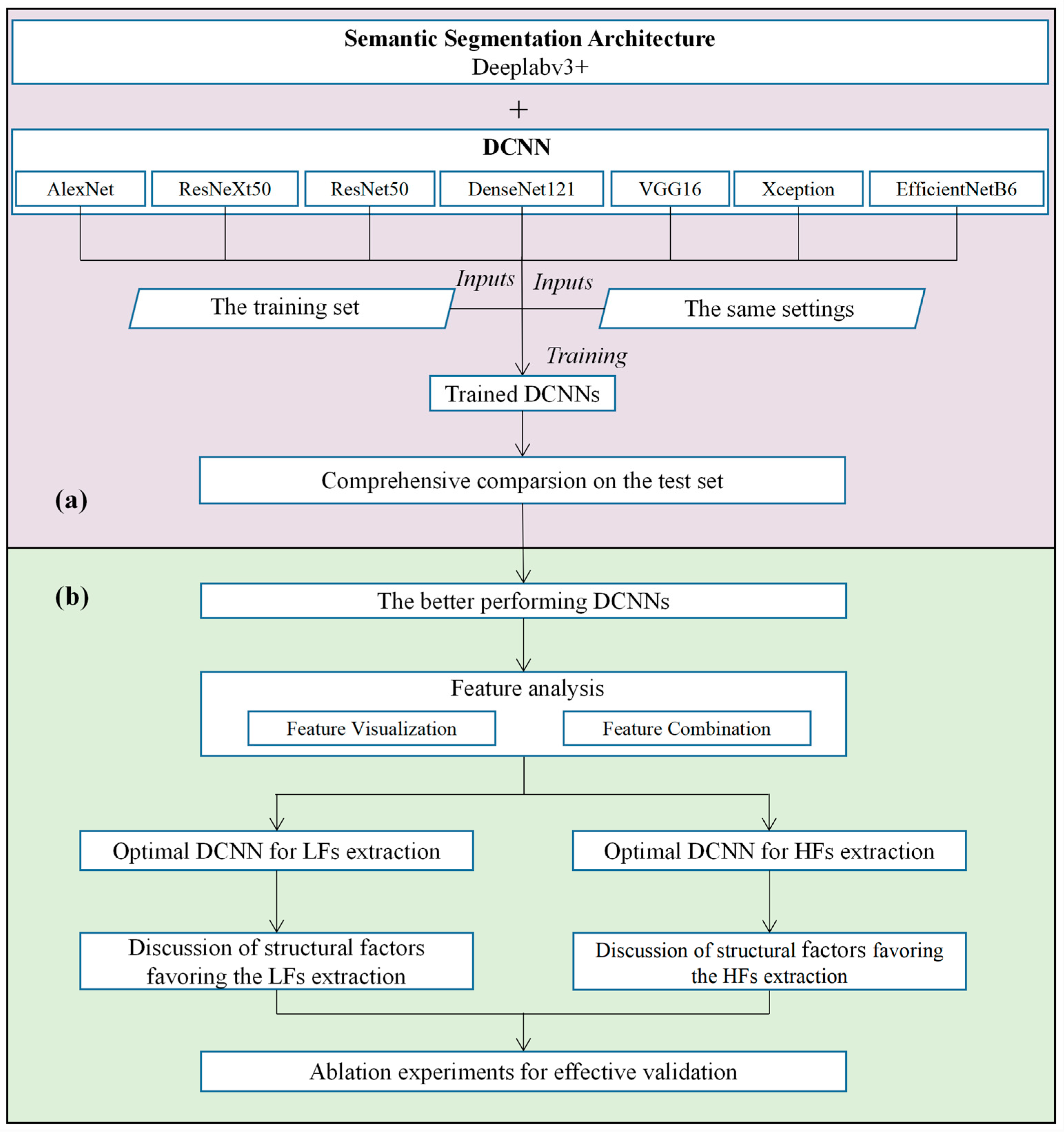
Figure 2 depicts the overall experimental procedure of our study, which comprises the following stages:
- (1)
- A comprehensive comparison of seven DCNNs for extracting PV arrays from HSRRS images (Figure 2a). These DCNNs are used as the backbone of the DeeplabV3_plus architecture to build seven semantic segmentation models. Then, these models are trained in the same way and compared on a unified dataset to gain insight into the differences between DCNNs.
- (2)
- An investigation of structural factors that favor the extraction of PV array features (Figure 2b). Both LFs and HFs are important for the extraction of PV arrays [36]. In this phase, we first analyze the differences between the better performing DCNNs in terms of LFs and HFs through feature visualization and combination. Then, through the structural analysis of the DCNNs with the best extraction of LFs and HFs, we identify the structural factors that favor the extraction of LFs and HFs and confirm their validity through ablation experiments.
3.1. Combination of the DCNNs and the DeeplabV3_Plus Architecture
Seven DCNNs—AlexNet, VGG16, ResNet50, ResNeXt50, DenseNet121, Xception, and EfficientNetB6—are selected for experiments based on the development trend of DCNNs. AlexNet is considered to be the cornerstone of the new generation of DCNNs. After AlexNet, VGG-Net, ResNet, and DenseNet are typical representatives that improve DCNN performance by increasing the network depth. In addition to increasing the depth, the effect of using multi-branch convolutional structures was also investigated. ResNeXt is representative of this, using group convolution (i.e., multiple parallel convolutional layers) instead of the normal convolution of ResNet to obtain richer features. Meanwhile, Xception uses a more extreme form of group convolution, known as separable convolution, for effective feature extraction. More recently, the incorporation of attention mechanisms has gained popularity to improve the feature extraction capabilities of DCNNs. EfficientNet is a notable example, which introduces the attention mechanism of SENet [37] to enable DCNNs to focus on the acquisition of useful information.
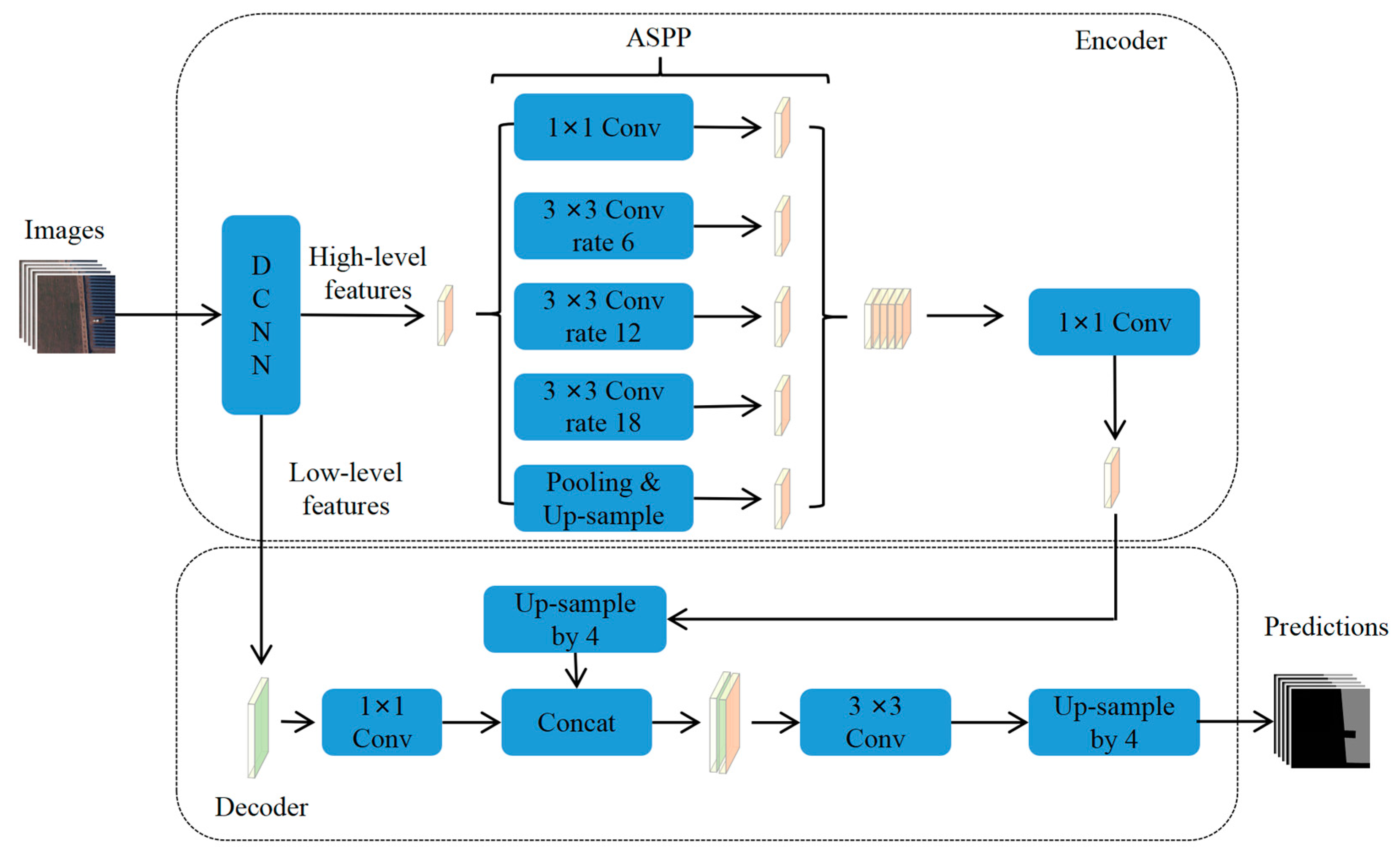
For the semantic segmentation architecture, DeeplabV3_plus is chosen due to its robust performance in extracting PV arrays from HSRRS images [35]. DeeplabV3_plus uses a standard encoder-decoder architecture (Figure 3). In the encoder, the final convolutional layer of the DCNN extracts the HFs. These features are then passed to Atrous Spatial Pyramid Pooling (ASPP) for the further extraction of multi-scale features. In the decoder, one input is the LFs extracted by the DCNN, while the other input is the output features of the ASPP after convolution and upsampling. In order to obtain features with the same size as the original image, these two inputs are combined and subsequently processed by convolution and upsampling operations. The features are then classified as PV or non-PV on a pixel-by-pixel basis.
For details on the combination of the DCNNs and the DeeplabV3_plus architecture, the LFs input to the DeeplabV3_plus decoder is the last feature map with a spatial size of one-quarter of the original image, extracted by DCNNs. The HFs’ input to the ASPP are the output feature maps of the last convolutional layer of the DCNNs. To satisfy the ASPP’s requirement that the spatial size of the input feature maps is one-sixteenth of the size of the original image, we remove the last downsampling operation of the convolutional part of the DCNNs (before removal, the spatial size of the output feature maps of the last convolutional layer is one-thirty-second of the original image).
3.2. Training and Evaluation of DCNNs
In this study, we develop the DCNNs using the pytorch-1.10 machine learning library in a Python environment. The training and evaluation processes are accelerated using the CUDA Toolkit 11.3 and NVIDIA Tesla V100 GPUs.
During the training, the DCNNs are trained from scratch using the training set without pre-trained weights. The batch size and the training epochs are set to 8 and 60, respectively. The Adam optimizer [38] is used to adjust the parameters of the DCNNs. The learning rate is given an initial value of 1 × 10⁻³, and subsequently reduced according to the conventional cosine recession strategy (Equation (1)). The loss function is a binary cross-entropy. To acquire an optimal generalization ability on the validation set, we store the DCNNS that have the minimum validation loss.
where presents the current epoch and LR stands for the learning rate.
In the evaluation, we use the test set to assess the DCNNs and compare their PV array extraction performance. Four common metrics in image segmentation tasks are employed to evaluate the performance of DCNN [39]: intersection over union (IoU), f1 score, recall, and precision. Precision indicates the proportion of actual PV array pixels among those identified as PV array pixels by the model (Equation (2)). Recall describes the percentage of PV array pixels correctly predicted by the model out of the actual PV array pixels (Equation (3)). The F1 score is the harmonic mean of precision and recall (Equation (4)). IoU is the intersection over the union ratio between the PV array pixels predicted by the model and the actual PV array pixels (Equation (5)).
where (true positive) signifies that the PV pixels were correctly identified by the model; (false negative) signifies that the PV pixels were misclassified as non-PV pixels by the model; (false positive) denotes non-PV pixels that are mistakenly classified as PV by the model.
3.3. Feature Visualization
To analyze the differences in the LFs and HFs extracted by DCNNs, we use LayerCAM [40] to create their class activation maps, while analyzing their attention regions of PV arrays on the images by visualizing the class activation maps.
LayerCAM is an effective method that generates class activation maps for different levels of features extracted by DCNNs. Specifically, for the kth feature map () in the given level features (), LayerCAM retains the positive gradient and eliminates the negative gradient in its backward gradient (), using it as the weight of (), as shown in the following equation:
where ReLU stands for rectified linear unit, which preserves positive values and sets negative values to 0.
To obtain the class activation map of , LayerCAM calculates a weighted activation value of each position in by multiplying it with its corresponding weight , and then sums these values along the channels and eliminates negative values by ReLU, as shown in the following equation:
This method assigns weights to each position of the features based on the gradient. Therefore, the resulting class activation maps can effectively highlight the attentional regions of PV arrays within the features.
3.4. Feature Combination
In order to further explore the differences in the LFs and HFs extracted by different DCNNs, we construct new models by combining different levels of features extracted by different DCNNs, and compare their performance with the corresponding DCNNs.
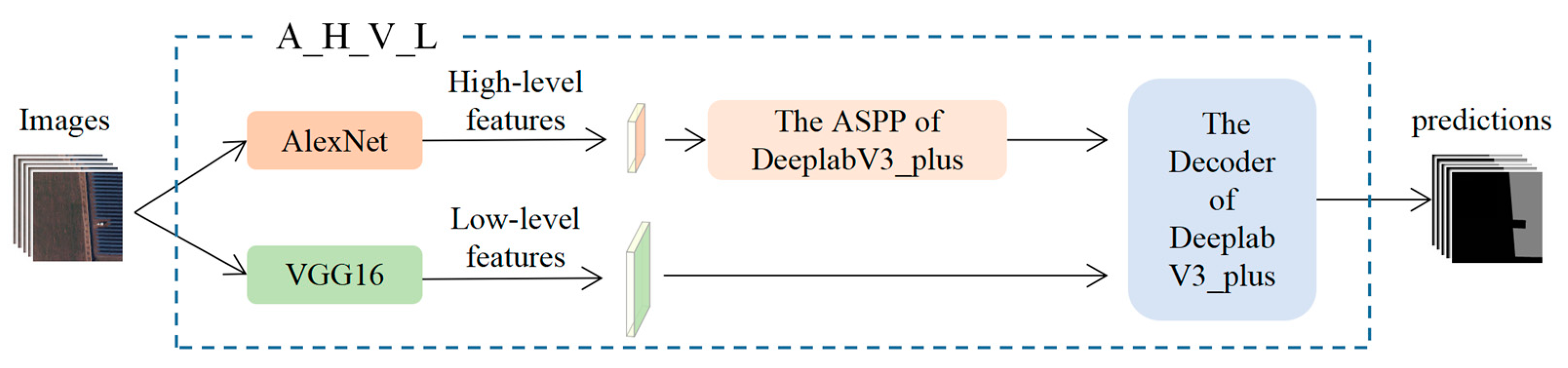
To compare the differences between the features extracted by AlexNet and VGG16, we construct a new model, A_H_V_L, by feeding the LFs extracted by the trained VGG16 into the decoder of DeeplabV3_Plus and the HFs extracted by the trained AlexNet into the ASPP of DeeplabV3_Plus (Figure 4). Here, A and V denote AlexNet and VGG16, respectively, and L and H denote the LFs and HFs, respectively. Other new models constructed by feature combination are similarly named. Note that the parameters of VGG16 and AlexNet in A_H_V_L are fixed, meaning that the LFs used in A_H_V_L are identical to those used in the trained VGG16, and the LFs used in A_H_V_L are identical to those used in the trained AlexNet.
In this case, the main difference of A_H_V_L compared to AlexNet is that it uses the LFs extracted by VGG16 for PV array extraction. Therefore, if A_H_V_L exhibits a performance improvement over AlexNet, it indicates that the LFs obtained by VGG16 are superior to those obtained by AlexNet in terms of PV array extraction performance. Similarly, if A_H_V_L shows an improvement over VGG16, it implies that the HFs extracted by AlexNet have a better performance for PV extraction than the HFs extracted by VGG16.
4. Comparison of Different DCNNs
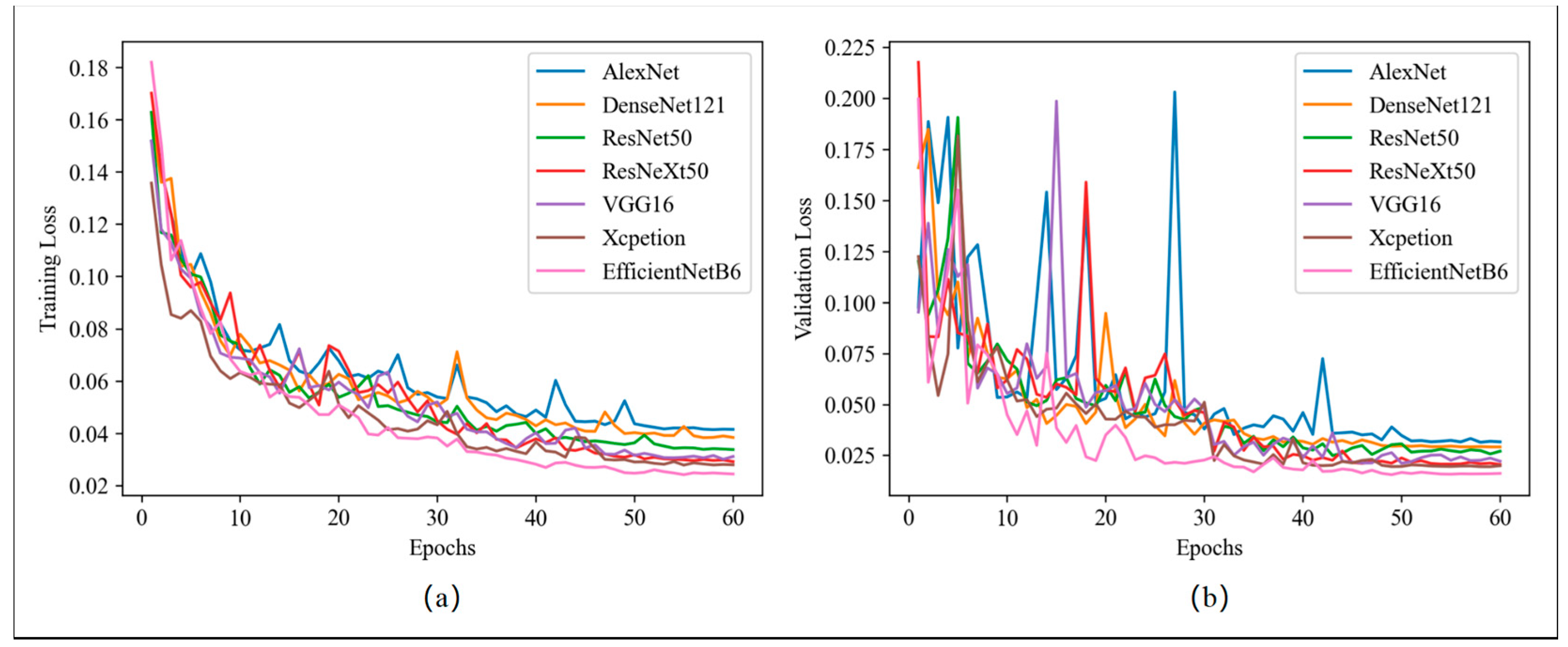
Figure 5 illustrates the loss curves of the DCNNs in the DeeplabV3_plus architecture. As shown in Figure 5a, EfficientNetB6 has the lowest ultimate training loss among the DCNNs, with a value of approximately 0.03. The final training losses of Xception, ResNeXt50, and VGG16 are almost indistinguishable and slightly higher than that of EfficientNetB6. In contrast, ResNet50, DenseNet121, and AlexNet have successively larger final training losses, all of which are significantly higher than those of the other four DCNNs. Regarding the validation loss (Figure 5b), all DCNNs show noticeable fluctuations in the first 50 epochs resulting from the reduced batch size, but they generally show a decreasing trend. The relative performance of the DCNNs in the final validation loss is comparable to that in the final training loss. In addition, due to the data augmentation operation, none of the DCNNs show an increasing trend in validation loss, indicating that there is no overfitting.
Table 1 lists the performance of each DCNN in the DeeplabV3_plus architecture. Overall, EfficientNetB6 outperforms the other DCNNs, achieving the highest values for recall, f1 score, and IoU. ResNeXt50, VGG16, and Xception perform similarly and have lower IoU and f1 scores than EfficientNetB6. However, VGG16 achieves the highest precision values. The remaining DCNNs exhibit poor performance across all metrics, with IoU values at least 1.4% lower than EfficientNetB6. It is noteworthy that ResNet50 does not perform well, despite having a deeper network structure and more parameters than VGG16. This suggests that the network depth and number of parameters are not the main factors influencing the performance of DCNNs in the PV array identification from HSRRS images.
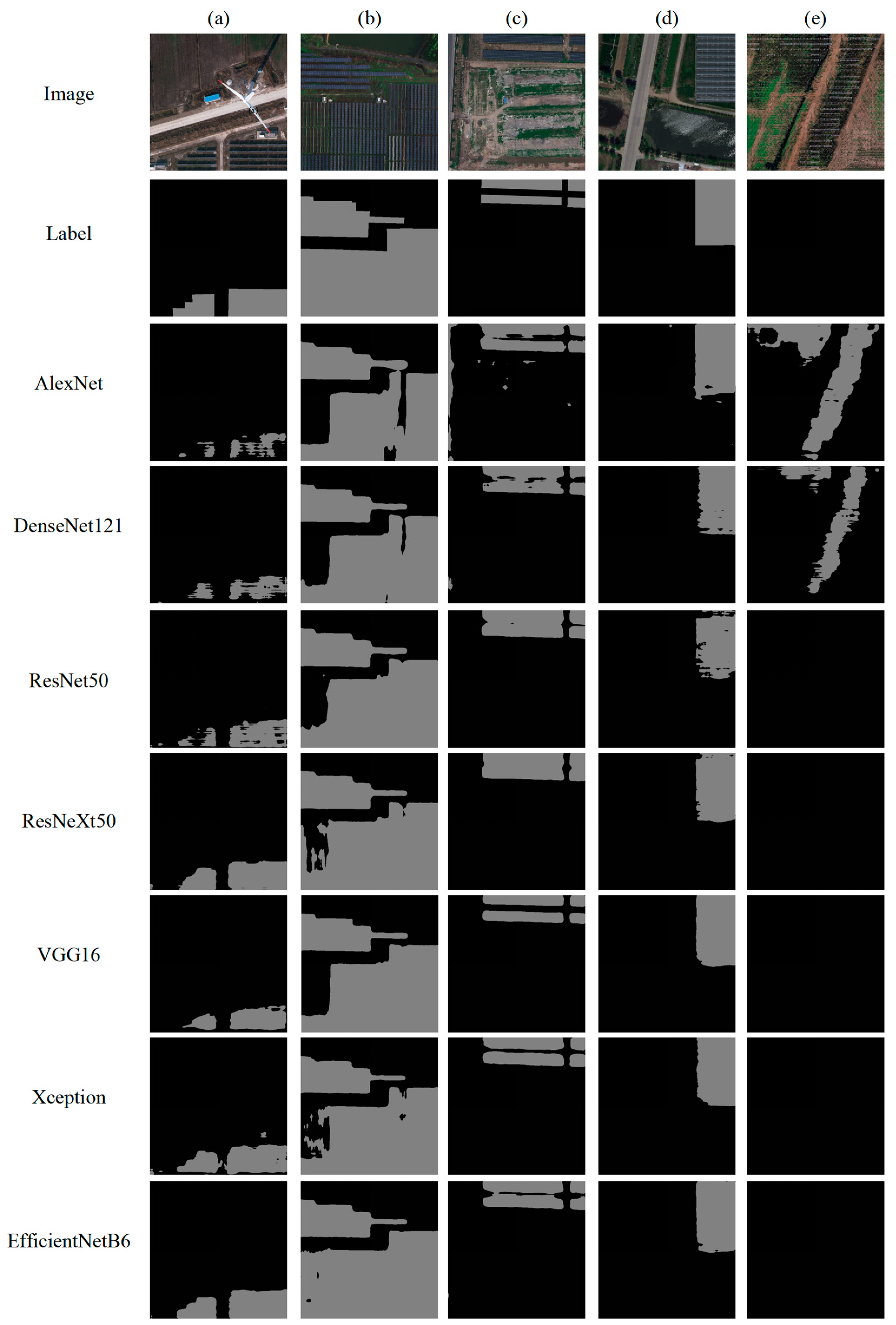
Figure 6 presents the PV arrays extracted by different DCNNs under the DeeplabV3_plus architecture. EfficientNetB6 exhibits the highest overall performance, demonstrating the complete extraction of high-tilt PV arrays (Figure 6a,b) without being affected by the PV rack interference (Figure 6e). Xception and ResNeXt50 display a slightly less accurate performance than EfficientNetB6, mainly owing to their incomplete extraction of high-tilt PV arrays (Figure 6a,b). In grassy areas, VGG16 fails to detect high-tilt PV arrays (Figure 6b). However, it excels at capturing the edges of PV arrays (Figure 6c,d). On the other hand, ResNet50, Dense-Net121, and AlexNet exhibit overall insufficient extraction. In particular, only DenseNet121 and AlexNet incorrectly identify the roadside guardrail (Figure 6c) and the PV racks (Figure 6e)as PV arrays.
Table 2 shows the number of parameters, depth, inference time, and memory usage of each DCNN under the DeeplabV3_plus architecture. AlexNet, VGG16, Xception, ResNet50, ResNext50, DenseNet121, and EfficientNetB6 in order of increasing depth. With the exception of DenseNet121, the number of parameters and the inference time of DCNNs tend to increase with their depth. In addition, AlexNet has the lowest memory usage, requiring less than 0.2 GB. ResNet50, Xception, DenseNet121, VGG16, and ResNeXt50 consume progressively more memory, but all being below 1 GB. In contrast, EfficientNetB6 requires over 2 GB of memory.
We also compare the PV array extraction performance of different DCNNs in the U-Net architecture. As shown in Table 3, EfficientNetB6 is still the best performer, with the highest values for recall, f1 score, and IoU. Xception and ResNeXt50 perform slightly worse than EfficientNetB6, but their IoU values are still above 94%. In comparison, VGG16 has an IoU value of 93.91%, higher than AlexNet, ResNet50, and DenseNet121. Replacing the architecture of DeeplabV3_plus with U-Net does not alter the better performance of EfficientNetB6, Xception, ResNeXt50, and VGG16 than the other DCNNs, indicating that the performance difference of DCNNs is not affected by the architectures.
5. Structural Factors Favoring the PV Array Feature Extraction
To improve the accuracy of PV array extraction from HSRRS images using DCNNs, we investigate the structural factors that contribute to PV array feature extraction by analyzing the differences in features and structures among the better performing DCNNs.
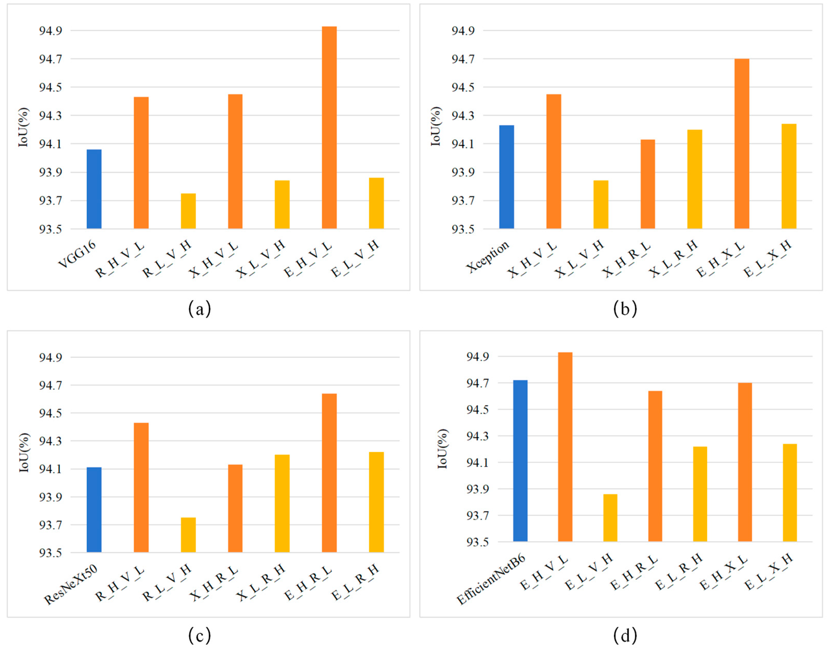
As shown in Table 2, VGG16, Xception, ResNeXt50, and EfficientNetB6 outperform the other three DCNNs. Therefore, we first analyze the feature differences of these four DCNNs based on feature combinations. Specifically, we develop twelve new models by combining different levels of features extracted by these four DCNNs. We then compare them with VGG16, Xception, ResNeXt50, and EfficientNetB6 on the test set (Figure 7). The following information can be derived from Figure 7:
- (1)
- VGG16 performs best in extracting the LFs of the PV array, as the IoU value of VGG16 is higher than those of R_L_V_H, X_L_V_H_ and E_L_V_H (Figure 7a).
- (2)
- (3)
- EfficientNetB6 shows the best ability in extracting the HFs of PV arrays, as it outperforms the new models using the HFs extracted by the other DCNNs (Figure 7d).
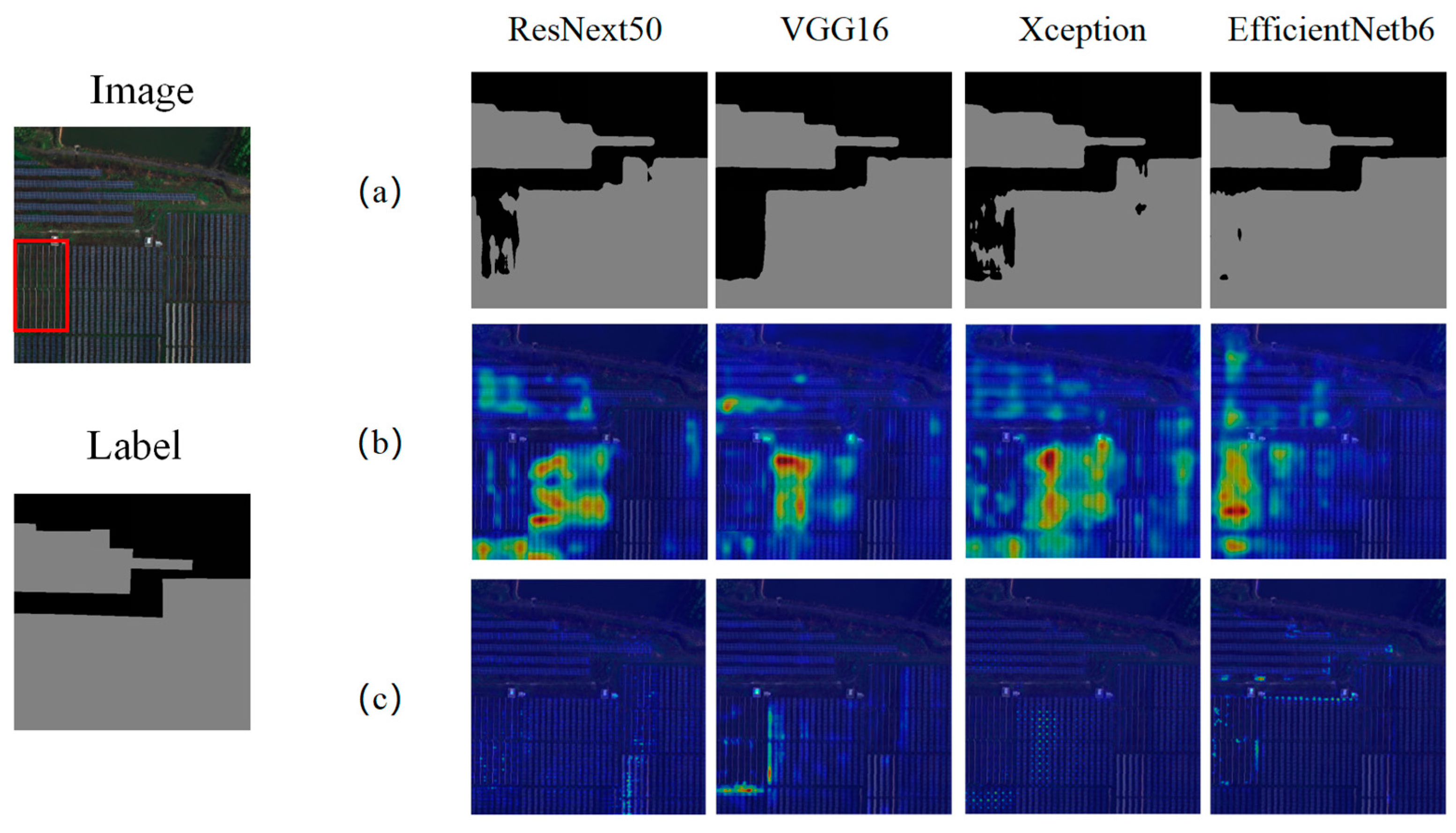
To understand the optimal performance of VGG16 for LF extraction and efficientNetB6 for HFs extraction, we generate class activation maps for LFs and HFs extracted by VGG16, Xception, ResNeXt50, and EfficientNetB6 using the LayerCAM method (Figure 8 and Figure 9).
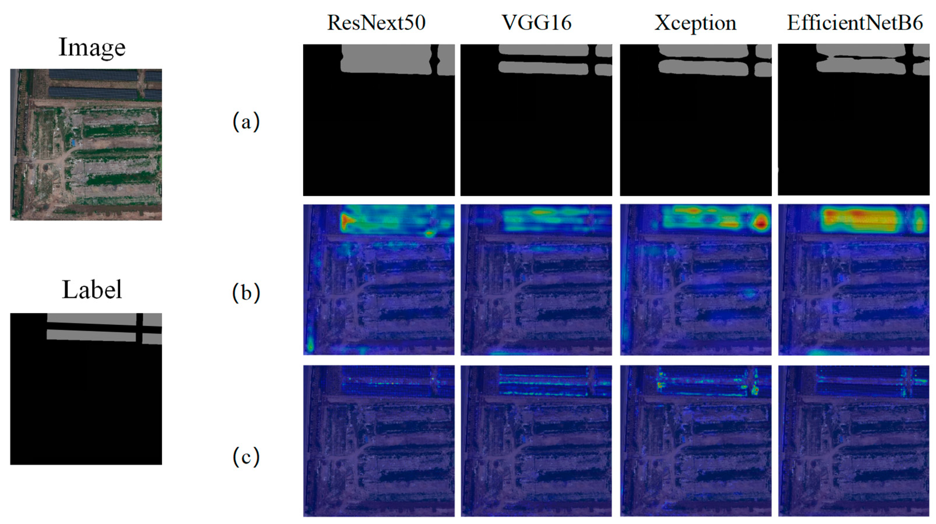
For the high-tilt PV array on grass (red square area in Figure 8), EfficientNetB6 has the optimal extraction (Figure 8a), because its HFs provide a stronger and more complete perception than those extracted by other DCNNs (Figure 8b). In addition, although VGG16 cannot detect the high-tilt PV arrays, its LFs are sensitive to the edges of this part of the PV arrays (Figure 8c).
For PV arrays on saline land (Figure 9), the HFs extracted by all DCNNs pay attention to them, while the attention of the HFs extracted by EfficientNetB6 is significantly stronger (Figure 9b). In addition, the LFs extracted by VGG16, which accurately detect the edges of the PV arrays, perform the best (Figure 9c).
The extraction capability of VGG16 on the LFs of PV arrays may be due to its first feature extraction block without downsampling. Since there is no downsampling undertaken, this type of block has a small receptive field when extracting features from the original image. As a result, it can perceive spatial features, such as textures and edges, in a more detailed manner, thus improving the fine extraction of object contours [41].
The extraction capability of EfficientNetB6 on the HFs of PV arrays may be due to its use of separable convolution (group convolution) and the SENet attention mechanism. Group convolution is more effective in extracting diverse features and may lead to the better extraction of HFs [34], as evidenced by the superior performance of ResNeXt50 over ResNet50 (Table 2). In addition, the attention mechanism allows the DCNN to focus on effective features and reduce the interference of redundant information, which improves the performance of the DCNN for object extraction [42].
To verify the above conjecture, we perform additional ablation experiments to investigate the effect of the first feature extraction block without downsampling on LFs’ extraction, and the effect of the separable convolution and attention mechanism on HFs’ extraction. The ablation experiments consist of the following steps:
- (1)
- Construction of three DCNNs: VGG16 with downsampling in the first feature extraction block (VD), EfficientNetB6 without separable convolution (EW/OS), EfficientNetB6 without attention mechanism (EW/OA). Note that VD is constructed by setting the stride of the first convolutional layer of VGG16 to 2, while eliminating the first Maxpooling layer of VGG16
- (2)
- Integrate these three DCNNs into the DeeplabV3_plus architecture, and training them using the training set and settings described in Section 3.2.
- (3)
- Construction of V_H_VD_L by combining the HFs extracted by the trained VGG16 and the LFs extracted by the trained VD; EW/OS_H_E_L by combining the HFs extracted by the trained EW/OS and the LFs extracted by the trained EfficientNetB6. EW/OA_H_E_L by combining the HFs extracted by the trained EW/OA and the LFs extracted by the trained EfficientNetB6.
- (4)
- Performance comparison between V_H_VD_L, VGG16, EW/OS_H_E_L, EW/OA_H_E_L, and EfficientNetB6.
As shown in Table 4, VGG16 outperforms V_H_VD_L in all metrics, indicating that the first feature extraction block without downsampling helps in extracting the LFs of the PV arrays. Furthermore, the inferior performance of EW/OS_H_E_L and EW/OA_H_E_L as compared to EfficientNetB6 confirms the importance of separable convolution and attention mechanisms in extracting the HFs of PV arrays.
6. Discussion
In this study, we compare the performance of seven DCNNs in extracting PV arrays from HSRRS images. Our results demonstrate that EfficientNetB6, VGG16, ResNeXt50, and Xception outperform AlexNet, ResNet50, and DenseNet121. Similar to our work, Costa et al. [43] also reported the superior PV array extraction performance of EfficientNet over ResNet in a comparative experiment. This provides additional evidence of performance differences between different DCNNs and highlights the need for comparisons. However, their analysis was limited to ResNet and EfficientNet, and was performed only on medium-resolution Sentinel-2 images. The performance of PV array extraction is significantly affected by the spatial resolution of the image [44]. Therefore, a comparison on HSRRS images could broaden the understanding of PV array extraction using deep learning approaches.
In addition, this study identifies three structural elements that facilitate PV array feature extraction: the first feature extraction block without downsampling, separable convolution, and attention mechanisms. Previous studies have also tentatively investigated the impact of attention mechanisms on PV array extraction. For instance, Zhu et al. [45] demonstrated the beneficial effect of the dual attention mechanism [46] on PV array extraction. Jie et al. [22] improved the accuracy of PV array extraction by using their self-designed spatial attention mechanism. Their study supports our findings regarding the effectiveness of the attention mechanism. However, unlike them, we argue that the attention mechanism enhances the ability of DCNNs to extract the HFs of PV arrays, thus improving the performance. Moreover, we emphasize the importance of the first feature extraction block without downsampling for obtaining the LFs of PV arrays and the significance of separable convolution for extracting the HFs of PV arrays.
Recently, Tan et al. [28] improved the accuracy of PV array extraction by integrating the color features and geometric structural features of PV arrays as priors into the DCNN. In essence, this approach is similar to the current study in that it seeks to improve the performance of the DCNN by enhancing its ability to extract PV array features. The difference lies in our exploration of the structural factors conducive to PV feature extraction, rather than the fusion methods of a priori features. Compared with their study, our research provides a direction for designing a DCNN structure capable of accurately extracting PV arrays.
In summary, previous research has confirmed the validity of certain findings in the current study, while the differences observed highlight the unique insights of the present study.
7. Conclusions
In this study, we conduct a comprehensive comparison of seven representative DCNNs-AlexNet, VGG16, ResNet50, ResNeXt50, DenseNet121, Xception, and Efficient-NetB6-in the task of extracting PV arrays from HSRRS images. The results show that the EfficientNetB6, VGG16, Xception, and ResNeXt50 outperform other DCNNs, achieving IoU values above 94%. Furthermore, EfficientNetB6 exhibits the best performance among these four DCNNs, but also the highest model complexity. In contrast, VGG16, Xception, and ResNeXt50 achieve a better balance between performance and complexity.
In addition, by examining the differences in features and structure of the better performing DCNNs, we explore the structural factors that contribute to the extraction of PV array features. Our findings indicate that the first feature extraction block without downsampling improves the ability of the DCNN to extract the LFs of PV arrays, resulting in an approximately 0.25% increase in IoU values. In addition, the separable convolution and attention mechanisms play a key role in improving the HFs’ extraction of DCNN, resulting in a 0.7% and 0.4% increase in IoU values, respectively.
Our study provides valuable insights into the impact of DCNN structures on the extraction of PV arrays from HSRRS images. These findings have significant implications for the selection of appropriate DCNNs and the design of robust DCNNs tailored for the accurate and efficient extraction of PV arrays. In future research, we plan to integrate favorable structural factors to construct robust DCNNs for the extraction of PV arrays from HSRRS images. In addition, we noticed that transfer learning is an effective method for improving the performance of DCNNs. Therefore, we will further explore how to improve the performance of extracting PV arrays from HSRRS images using excellent transfer learning methods such as PADM [47].
Author Contributions
L.L.: Writing—original draft, Data Curation, Formal analysis, and Methodology. N.L.: Visualization, Validation, Conceptualization, Writing—review and editing, Funding acquisition, Project administration. J.Q.: Investigation, Software. H.J.: Resources, Visualization, Writing—review and editing. All authors have read and agreed to the published version of the manuscript.
Funding
This study was funded by the National Natural Science Foundation of China (grant no. 41971312), the Third Xinjiang Scientific Expedition Program (Grant No. 2021xjkk0303) and the Key Project of Innovation LREIS (KPI009).
Data Availability Statement
PV array sample dataset is publicly available at https://zenodo.org/record/5171712 (1 September 2023).
Acknowledgments
We are grateful to the Geographic Information Center of Jiangsu Province for providing computational resources, and the GitHub user Bubbliiiing for sharing the DeeplabV3_plus code (https://github.com/bubbliiiing/deeplabv3-plus-pytorch, last accesse: 1 August 2023).
Conflicts of Interest
The authors declare no conflict of interest.
References
- Olson, C.; Lenzmann, F. The social and economic consequences of the fossil fuel supply chain. MRS Energy Sustain. 2016, 3, E6. [Google Scholar] [CrossRef]
- Aman, M.M.; Solangi, K.H.; Hossain, M.S.; Badarudin, A.; Jasmon, G.B.; Mokhlis, H.; Bakar, A.H.A.; Kazi, S.N. A review of Safety, Health and Environmental (SHE) issues of solar energy system. Renew. Sustain. Energy Rev. 2015, 41, 1190–1204. [Google Scholar] [CrossRef]
- Yan, J.Y.; Yang, Y.; Campana, P.E.; He, J.J. City-level analysis of subsidy-free solar photovoltaic electricity price, profits and grid parity in China. Nat. Energy 2019, 4, 709–717. [Google Scholar] [CrossRef]
- International Renewable Energy Agency. Renewable Capacity Statistics. 2022. Available online: https://www.irena.org/Publications/2023/Jul/Renewable-energy-statistics-2023 (accessed on 31 August 2023).
- Lv, T.; Yang, Q.; Deng, X.; Xu, J.; Gao, J. Generation Expansion Planning Considering the Output and Flexibility Requirement of Renewable Energy: The Case of Jiangsu Province. Front. Energy Res. 2020, 8, 39. [Google Scholar] [CrossRef]
- Nassar, Y.F.; Hafez, A.A.; Alsadi, S.Y. Multi-Factorial Comparison for 24 Distinct Transposition Models for Inclined Surface Solar Irradiance Computation in the State of Palestine: A Case Study. Front. Energy Res. 2020, 7, 163. [Google Scholar] [CrossRef]
- Manfren, M.; Nastasi, B.; Groppi, D.; Garcia, D.A. Open data and energy analytics—An analysis of essential information for energy system planning, design and operation. Energy 2020, 213, 118803. [Google Scholar] [CrossRef]
- Feng, D.; Chen, H.; Xie, Y.; Liu, Z.; Liao, Z.; Zhu, J.; Zhang, H. GCCINet: Global feature capture and cross-layer information interaction network for building extraction from remote sensing imagery. Int. J. Appl. Earth Obs. Geoinf. 2022, 114, 103046. [Google Scholar] [CrossRef]
- Zefri, Y.; Sebari, I.; Hajji, H.; Aniba, G. Developing a deep learning-based layer-3 solution for thermal infrared large-scale photovoltaic module inspection from orthorectified big UAV imagery data. Int. J. Appl. Earth Obs. Geoinf. 2022, 106, 102652. [Google Scholar] [CrossRef]
- Li, P.; Zhang, H.; Guo, Z.; Lyu, S.; Chen, J.; Li, W.; Song, X.; Shibasaki, R.; Yan, J. Understanding rooftop PV panel semantic segmentation of satellite and aerial images for better using machine learning. Adv. Appl. Energy 2021, 4, 100057. [Google Scholar] [CrossRef]
- Zheng, J.; Yuan, S.; Wu, W.; Li, W.; Yu, L.; Fu, H.; Coomes, D. Surveying coconut trees using high-resolution satellite imagery in remote atolls of the Pacific Ocean. Remote Sens. Environ. 2023, 287, 113485. [Google Scholar] [CrossRef]
- Carletti, V.; Greco, A.; Saggese, A.; Vento, M. An intelligent flying system for automatic detection of faults in photovoltaic plants. J. Ambient Intell. Humaniz. Comput. 2020, 11, 2027–2040. [Google Scholar] [CrossRef]
- Grimaccia, F.; Leva, S.; Niccolai, A. PV plant digital mapping for modules’ defects detection by unmanned aerial vehicles. Iet Renew. Power Gener. 2017, 11, 1221–1228. [Google Scholar] [CrossRef]
- Jiang, W.; Tian, B.; Duan, Y.; Chen, C.; Hu, Y. Rapid mapping and spatial analysis on the distribution of photovoltaic power stations with Sentinel-1&2 images in Chinese coastal provinces. Int. J. Appl. Earth Obs. Geoinf. 2023, 118, 10328. [Google Scholar] [CrossRef]
- Xia, Z.; Li, Y.; Guo, X.; Chen, R. High-resolution mapping of water photovoltaic development in China through satellite imagery. Int. J. Appl. Earth Obs. Geoinf. 2022, 107, 10270. [Google Scholar] [CrossRef]
- Wu, A.N.; Biljecki, F. Roofpedia: Automatic mapping of green and solar roofs for an open roofscape registry and evaluation of urban sustainability. Landsc. Urban Plan. 2021, 214, 104167. [Google Scholar] [CrossRef]
- Ge, F.; Wang, G.; He, G.; Zhou, D.; Yin, R.; Tong, L. A Hierarchical Information Extraction Method for Large-Scale Centralized Photovoltaic Power Plants Based on Multi-Source Remote Sensing Images. Remote Sens. 2022, 14, 4211. [Google Scholar] [CrossRef]
- Sizkouhi, A.M.M.; Aghaei, M.; Esmailifar, S.M.; Mohammadi, M.R.; Grimaccia, F. Automatic Boundary Extraction of Large-Scale Photovoltaic Plants Using a Fully Convolutional Network on Aerial Imagery. IEEE J. Photovolt. 2020, 10, 1061–1067. [Google Scholar] [CrossRef]
- Zhang, H.; Tian, P.; Zhong, J.; Liu, Y.; Li, J. Mapping Photovoltaic Panels in Coastal China Using Sentinel-1 and Sentinel-2 Images and Google Earth Engine. Remote Sens. 2023, 15, 3712. [Google Scholar] [CrossRef]
- Chen, Z.; Kang, Y.; Sun, Z.; Wu, F.; Zhang, Q. Extraction of Photovoltaic Plants Using Machine Learning Methods: A Case Study of the Pilot Energy City of Golmud, China. Remote Sens. 2022, 14, 2697. [Google Scholar] [CrossRef]
- Chen, T.; Guestrin, C. XGBoost: A Scalable Tree Boosting System. In Proceedings of the 22nd ACM SIGKDD International Conference on Knowledge Discovery and Data Mining, San Francisco, CA, USA, 13–17 August 2016; pp. 785–794. [Google Scholar] [CrossRef]
- Jie, Y.S.; Ji, X.H.; Yue, A.Z.; Chen, J.B.; Deng, Y.P.; Chen, J.; Zhang, Y. Combined Multi-Layer Feature Fusion and Edge Detection Method for Distributed Photovoltaic Power Station Identification. Energies 2020, 13, 6742. [Google Scholar] [CrossRef]
- Chen, L.C.E.; Zhu, Y.K.; Papandreou, G.; Schroff, F.; Adam, H. Encoder-Decoder with Atrous Separable Convolution for Semantic Image Segmentation. In Proceedings of the European Conference on Computer Vision (ECCV), Munich, Germany, 8–14 September 2018; pp. 833–851. [Google Scholar] [CrossRef]
- Simonyan, K.; Zisserman, A. Very Deep Convolutional Networks for Large-Scale Image Recognition. arXiv 2014, arXiv:1409.1556. [Google Scholar] [CrossRef]
- He, K.M.; Gkioxari, G.; Dollar, P.; Girshick, R. Mask R-CNN. In Proceedings of the IEEE International Conference on Computer Vision (ICCV), Venice, Italy, 22–29 October 2017; pp. 2980–2988. [Google Scholar] [CrossRef]
- He, K.; Zhang, X.; Ren, S.; Sun, J. Deep Residual Learning for Image Recognition. In Proceedings of the IEEE Conference on Computer Vision and Pattern Recognition (CVPR), Las Vegas, NV, USA, 27–30 June 2016; pp. 770–778. [Google Scholar] [CrossRef]
- Ronneberger, O.; Fischer, P.; Brox, T. U-Net: Convolutional Networks for Biomedical Image Segmentation. In Proceedings of the Medical Image Computing and Computer-Assisted Intervention (MICCAI), Munich, Germany, 5–9 October 2015; pp. 234–241. [Google Scholar] [CrossRef]
- Tan, H.; Guo, Z.; Zhang, H.; Chen, Q.; Lin, Z.; Chen, Y.; Yan, J. Enhancing PV panel segmentation in remote sensing images with constraint refinement modules. Appl. Energy 2023, 350, 121757. [Google Scholar] [CrossRef]
- Garcia-Garcia, A.; Orts-Escolano, S.; Oprea, S.; Villena-Martinez, V.; Martinez-Gonzalez, P.; Garcia-Rodriguez, J. A survey on deep learning techniques for image and video semantic segmentation. Appl. Soft Comput. 2018, 70, 41–65. [Google Scholar] [CrossRef]
- Atik, S.O.; Atik, M.E.; Ipbuker, C. Comparative research on different backbone architectures of DeeplabV3_plus for building segmentation. J. Appl. Remote Sens. 2022, 16, 024510. [Google Scholar] [CrossRef]
- Krizhevsky, A.; Sutskever, I.; Hinton, G. ImageNet Classification with Deep Convolutional Neural Networks. Commun. ACM 2012, 60, 84–90. [Google Scholar] [CrossRef]
- Chollet, F. Xception: Deep Learning with Depthwise Separable Convolutions. In Proceedings of the IEEE Conference on Computer Vision and Pattern Recognition (CVPR), Honolulu, HI, USA, 21–26 July 2017; pp. 1800–1807. [Google Scholar] [CrossRef]
- Huang, G.; Liu, Z.; Maaten, L.V.D.; Weinberger, K.Q. Densely Connected Convolutional Networks. In Proceedings of the IEEE Conference on Computer Vision and Pattern Recognition (CVPR), Honolulu, HI, USA, 21–26 July 2017; pp. 2261–2269. [Google Scholar] [CrossRef]
- Xie, S.; Girshick, R.; Dollár, P.; Tu, Z.; He, K. Aggregated Residual Transformations for Deep Neural Networks. In Proceedings of the IEEE Conference on Computer Vision and Pattern Recognition (CVPR), Honolulu, HI, USA, 21–26 July 2017; pp. 5987–5995. [Google Scholar] [CrossRef]
- Jiang, H.; Yao, L.; Lu, N.; Qin, J.; Liu, T.; Liu, Y.; Zhou, C. Multi-resolution dataset for photovoltaic panel segmentation from satellite and aerial imagery. Earth Syst. Sci. Data 2021, 13, 5389–5401. [Google Scholar] [CrossRef]
- Shelhamer, E.; Long, J.; Darrell, T. Fully Convolutional Networks for Semantic Segmentation. Proc. IEEE Trans. Pattern Anal. Mach. Intell. 2017, 39, 640–651. [Google Scholar] [CrossRef]
- Hu, J.; Shen, L.; Sun, G. Squeeze-and-Excitation Networks. In Proceedings of the IEEE/CVF Conference on Computer Vision and Pattern Recognition, Salt Lake City, UT, USA, 18–23 June 2018; pp. 7132–7141. [Google Scholar] [CrossRef]
- Kingma, D.P.; Ba, J. Adam: A method for stochastic optimization. arXiv 2014, arXiv:1412.6980. [Google Scholar] [CrossRef]
- Wu, G.; Guo, Z.; Shi, X.; Chen, Q.; Xu, Y.; Shibasaki, R.; Shao, X. A Boundary Regulated Network for Accurate Roof Segmentation and Outline Extraction. Remote Sens. 2018, 10, 1195. [Google Scholar] [CrossRef]
- Jiang, P.T.; Zhang, C.B.; Hou, Q.; Cheng, M.M.; Wei, Y. LayerCAM: Exploring Hierarchical Class Activation Maps for Localization. IEEE Trans. Image Process. 2021, 30, 5875–5888. [Google Scholar] [CrossRef]
- Liu, T.; Yao, L.; Qin, J.; Lu, N.; Jiang, H.; Zhang, F.; Zhou, C. Multi-scale attention integrated hierarchical networks for high-resolution building footprint extraction. Int. J. Appl. Earth Obs. Geoinf. 2022, 109, 102768. [Google Scholar] [CrossRef]
- Lu, R.; Wang, N.; Zhang, Y.B.; Lin, Y.E.; Wu, W.Q.; Shi, Z. Extraction of Agricultural Fields via DASFNet with Dual Attention Mechanism and Multi-scale Feature Fusion in South Xinjiang, China. Remote Sens. 2022, 14, 2253–2275. [Google Scholar] [CrossRef]
- da Costa, M.V.C.V.; de Carvalho, O.L.F.; Orlandi, A.G.; Hirata, I.; de Albuquerque, A.O.; e Silva, F.V.; Guimarães, R.F.; Gomes, R.A.T.; Júnior, O.A.d.C. Remote Sensing for Monitoring Photovoltaic Solar Plants in Brazil Using Deep Semantic Segmentation. Energies 2021, 14, 2960. [Google Scholar] [CrossRef]
- Kruitwagen, L.; Story, K.T.; Friedrich, J.; Byers, L.; Skillman, S.; Hepburn, C. A global inventory of photovoltaic solar energy generating units. Nature 2021, 598, 604–610. [Google Scholar] [CrossRef]
- Zhu, R.; Guo, D.; Wong, M.S.; Qian, Z.; Chen, M.; Yang, B.; Chen, B.; Zhang, H.; You, L.; Heo, J.; et al. Deep solar PV refiner: A detail-oriented deep learning network for refined segmentation of photovoltaic areas from satellite imagery. Int. J. Appl. Earth Obs. Geoinf. 2023, 116, 103134. [Google Scholar] [CrossRef]
- Fu, J.; Liu, J.; Tian, H.; Li, Y.; Bao, Y.; Fang, Z.; Lu, H. Dual Attention Network for Scene Segmentation. In Proceedings of the IEEE/CVF Conference on Computer Vision and Pattern Recognition (CVPR), Long Beach, CA, USA, 16–20 June 2019; pp. 3141–3149. [Google Scholar] [CrossRef]
- Zheng, J.; Zhao, Y.; Wu, W.; Chen, M.; Li, W.; Fu, H. Partial Domain Adaptation for Scene Classification From Remote Sensing Imagery. IEEE Trans. Geosci. Remote Sens. 2023, 61, 1–17. [Google Scholar] [CrossRef]
Figure 1.
Samples of PV arrays from the dataset.

Figure 2.
Experimental procedure of this study. (a) The comparative analysis of seven DCNNs. (b) The investigation of structural factors that favor the extraction of PV array features. LFs denote low-level spatial features and HFs denote high-level semantic features.
Figure 2.
Experimental procedure of this study. (a) The comparative analysis of seven DCNNs. (b) The investigation of structural factors that favor the extraction of PV array features. LFs denote low-level spatial features and HFs denote high-level semantic features.

Figure 3.
DeeplabV3_plus architecture diagram.

Figure 4.
The new model (A_H_V_L) constructed by combining high-level semantic features extracted by AlexNet and low-level spatial features extracted by VGG16.
Figure 4.
The new model (A_H_V_L) constructed by combining high-level semantic features extracted by AlexNet and low-level spatial features extracted by VGG16.

Figure 5.
Loss curves of training (a) and validation (b) for DCNNs in the DeeplabV3_plus architecture.
Figure 5.
Loss curves of training (a) and validation (b) for DCNNs in the DeeplabV3_plus architecture.

Figure 6.
High-tilt PV arrays (a,b), panelized PV arrays (c,d), and PV racks (e) extracted by different DCNNs.
Figure 6.
High-tilt PV arrays (a,b), panelized PV arrays (c,d), and PV racks (e) extracted by different DCNNs.

Figure 7.
Comparison of IoU values between VGG16 and its corresponding new models (a), Xception and its corresponding new models (b), ResNeXt50 and its corresponding new models (c), EfficientNetB6 its corresponding new models (d) on the test set. X_H_R_L represents the new model that combines HFs extracted by Xception with LFs extracted by ResNeXt50, and other abbreviations have similar meanings.

Figure 8.
High-tilt PV arrays extracted by the DCNNs (a) and the class activation maps of LFs (b) and HFs (c).
Figure 8.
High-tilt PV arrays extracted by the DCNNs (a) and the class activation maps of LFs (b) and HFs (c).

Figure 9.
PV arrays extracted by the DCNNs on saline land (a) and the class activation maps of LFs (b) and HFs (c).
Figure 9.
PV arrays extracted by the DCNNs on saline land (a) and the class activation maps of LFs (b) and HFs (c).


Table 1.
Performance of each DCNN in the DeeplabV3_plus architecture.
| DCNN | Precision (%) | Recall (%) | F1 score (%) | IoU (%) |
|---|---|---|---|---|
| AlexNet | 95.69 | 96.45 | 96.07 | 92.44 |
| DenseNet121 | 95.85 | 96.76 | 96.30 | 92.86 |
| ResNet50 | 96.01 | 97.03 | 96.52 | 93.28 |
| ResNeXt50 | 96.21 | 97.74 | 96.97 | 94.11 |
| VGG16 | 96.59 | 97.30 | 96.94 | 94.06 |
| Xception | 96.28 | 97.79 | 97.03 | 94.23 |
| EfficientNetB6 | 96.47 | 98.12 | 97.29 | 94.72 |
Table 2.
The number of parameters, depths, inference time, and memory usage of DCNNs in the DeeplabV3_plus architecture.
Table 2.
The number of parameters, depths, inference time, and memory usage of DCNNs in the DeeplabV3_plus architecture.
| DCNN | Number of Parameters (Millions) | Depth | Inference Time (ms) | Memory Usage (GB) |
|---|---|---|---|---|
| AlexNet | 7.2 | 10 | 2.43 | 0.19 |
| DenseNet121 | 16.2 | 125 | 9.60 | 0.71 |
| ResNet50 | 40.4 | 54 | 8.08 | 0.65 |
| ResNeXt50 | 38.9 | 54 | 9.52 | 0.99 |
| VGG16 | 20.2 | 18 | 3.41 | 0.97 |
| Xception | 37.7 | 41 | 5.97 | 0.75 |
| EfficientNetB6 | 59.5 | 141 | 19.95 | 2.47 |
The memory usage and the inference time refer to the memory and amount of time consumed by DCNNs during the inference process of a single image, respectively.
Table 3.
Performance of different DCNNs in the U-Net architecture.
| DCNN | Precision (%) | Recall (%) | F1 Score (%) | IoU (%) |
|---|---|---|---|---|
| AlexNet | 95.87 | 96.13 | 95.99 | 92.27 |
| DenseNet121 | 96.09 | 96.41 | 96.25 | 92.77 |
| ResNet50 | 96.19 | 96.68 | 96.43 | 93.09 |
| ResNeXt50 | 96.40 | 97.42 | 96.91 | 94.01 |
| VGG16 | 96.75 | 96.98 | 96.86 | 93.91 |
| Xception | 96.49 | 97.41 | 96.95 | 94.07 |
| EfficicentNetB6 | 96.59 | 97.84 | 97.22 | 94.59 |
Table 4.
Performance of V_H_VD_L, VGG16, EW/OS_H_E_L, EW/OA_H_E_L, and EfficientNetB6 in the DeeplabV3_plus architecture.
Table 4.
Performance of V_H_VD_L, VGG16, EW/OS_H_E_L, EW/OA_H_E_L, and EfficientNetB6 in the DeeplabV3_plus architecture.
| DCNN | Precision (%) | Recall (%) | F1 Score (%) | IoU (%) |
|---|---|---|---|---|
| V_H_VD_L | 96.44 | 96.25 | 96.82 | 93.83 |
| VGG16 | 96.59 | 97.30 | 96.94 | 94.06 |
| EW/OS_H_E_L | 96.30 | 97.54 | 96.92 | 94.02 |
| EW/OA_H_E_L | 96.32 | 97.86 | 97.08 | 94.33 |
| EfficientNetB6 | 96.47 | 98.12 | 97.29 | 94.72 |
V_H_VD_L represents the model constructed by combining the HFs extracted by VGG16 with the LFs extracted by VD, and other abbreviations have similar meanings.
Disclaimer/Publisher’s Note: The statements, opinions and data contained in all publications are solely those of the individual author(s) and contributor(s) and not of MDPI and/or the editor(s). MDPI and/or the editor(s) disclaim responsibility for any injury to people or property resulting from any ideas, methods, instructions or products referred to in the content. |
© 2023 by the authors. Licensee MDPI, Basel, Switzerland. This article is an open access article distributed under the terms and conditions of the Creative Commons Attribution (CC BY) license (https://creativecommons.org/licenses/by/4.0/).
Share and Cite
MDPI and ACS Style
Li, L.; Lu, N.; Jiang, H.; Qin, J. Impact of Deep Convolutional Neural Network Structure on Photovoltaic Array Extraction from High Spatial Resolution Remote Sensing Images. Remote Sens. 2023, 15, 4554. https://doi.org/10.3390/rs15184554
AMA Style
Li L, Lu N, Jiang H, Qin J. Impact of Deep Convolutional Neural Network Structure on Photovoltaic Array Extraction from High Spatial Resolution Remote Sensing Images. Remote Sensing. 2023; 15(18):4554. https://doi.org/10.3390/rs15184554
Chicago/Turabian StyleLi, Liang, Ning Lu, Hou Jiang, and Jun Qin. 2023. "Impact of Deep Convolutional Neural Network Structure on Photovoltaic Array Extraction from High Spatial Resolution Remote Sensing Images" Remote Sensing 15, no. 18: 4554. https://doi.org/10.3390/rs15184554
Note that from the first issue of 2016, this journal uses article numbers instead of page numbers. See further details here.