Increasing the Observability of Near Inertial Oscillations by a Future ODYSEA Satellite Mission

Abstract

Near Inertial Oscillations (NIOs) are ocean oscillations forced by intermittent winds. They are most energetic at mid-latitudes, particularly in regions with atmospheric storm tracks. Wind-driven, large-scale NIOs are quickly scattered by ocean mesoscale eddies (with sizes ranging from 100 to 400 km), causing a significant portion of the NIO energy to propagate into the subsurface ocean interior. This kinetic energy pathway illustrates that the wind energy input to NIO is critical for maintaining deep ocean stratification and thus closing the total energy budget, as emphasised by numerous modelling studies. However, this wind energy input to NIO remains poorly observed on a global scale. A remote sensing approach that observes winds and ocean currents co-located in time and space with high resolution is necessary to capture the intermittent air-sea coupling. The current satellite observations do not meet these requirements. This study assesses the potential of a new satellite mission concept, Ocean DYnamics and Surface Exchange with the Atmosphere (OSYSEA), to recover wind-forced NIOs from co-located winds and currents. To do this, we use an Observation System Simulation Experiment (OSSE) based on hourly observations of ocean surface currents and surface winds from five surface moorings covering latitudes from ${15}^{°}$ to ${50}^{°}$. ODYSEA wind and current observations are expected to have a spatial resolution of 10 km with about a 12 h sampling frequency in mid-latitudes. Results show that NIOs can be recovered with high accuracy using the ODYSEA spatial and temporal resolution, but only if observations are made over a wide area of 1800 km. A narrower swath (1000 km) may lead to significant aliasing.

1. Introduction

The ocean, as a stratified rotating fluid, supports several classes of high-frequency waves, from the Coriolis frequency (f), associated with Earth’s rotation, to the Brunt-Väisälä frequency (N), associated with ocean stratification. At mid-latitudes, where atmospheric storm tracks are located, these frequencies range from approximately ${10}^{-4}$s${}^{-1}$ for the Coriolis frequency to $3\times {10}^{-3}$s${}^{-1}$ for the Brunt-Väisälä frequency. A dispersion relation for these waves associates frequencies with length scales. In the context of the shallow water framework, this relationship is given by [1]:

$${\omega }^2=f^2(1+k^2{r}_d^2),$$

where $\omega$ denotes the wave frequency, k their horizontal wavenumber (i.e., the inverse of length scale), and $r_d$ a Rossby radius of deformation that characterizes the oceanic stratification and is of an infinite number of values depending on the vertical structure. Atmospheric winds can drive these wave classes if wind energy exists within the $f-N$ frequency band. High-frequency winds are characterized by a wavenumber spectrum that features energetic scales of the order of $\mathcal{O}$500–1000 km, significantly larger than the oceanic internal Rossby radii of deformation (less than 50 km). This implies that for oceanic motions directly induced by such winds, $k^2{r}_d^2$ is much smaller than 1, which elucidates that the frequency of the resulting wind-forced waves is near the Coriolis frequency. These large-scale near-inertial oscillations (NIO) are trapped within the surface mixed-layer (50–100 m deep), and thus, the mixed-layer can be regarded as an oscillator with frequency f. This resonance mechanism was recognized long ago [2,3,4]. The impact of “inertial” wind on NIOs has been revisited recently [5,6]. Consequently, using real wind time series observed on a weather ship, it was discovered that the resulting NIO kinetic energy is reduced by a factor of 1.5, 3, and 7 when the wind is averaged over 6, 12, and 14 h, respectively [5].

The wind energy input is determined by the scalar product of wind stresses and currents, which is also called wind work. The total wind work is estimated to be about 5 TW in the global ocean [7,8], a magnitude larger than the work completed by the steady large-scale winds on the general circulation (estimated to be 1 TW [9]). This total wind work includes three main contributions. The first one, which represents 28% of the total wind work, ∼1.4 TW, concerns the high-frequency contribution that forces internal gravity waves such as NIOs. This magnitude is within the range of values found by previous studies, but it is lower than those found by Liu et al. [10]. The two other contributions concern the one that forces or damps lower frequency motions (28%), such as mesoscale eddies, and the one that forces seasonally averaged currents (44%) [8,11]). The energy input to NIO, which mostly occurs in regions of atmospheric storm tracks [6,7] is critical to maintain the deep ocean stratification and therefore to close the total kinetic energy budget. However, how much of this wind-driven near-inertial energy penetrates into the deep ocean interior and where it penetrates is still a puzzle, although some progress has been made in the past 20 years. Thus, a significant part of the large-scale NIOs forced by large-sale winds is quickly scattered into smaller spatial scales by the potential vorticity of mesoscale eddies (with a 100–500 km size) [12]. Potential vorticity includes two main components: the relative vorticity, interpreted as the spin of the eddies, which is negative (positive) in anticyclonic (cyclonic) eddies, and the stratification, which is smaller (larger) in anticyclonic (cyclonic) eddies [12,13]. This explains why NIOs at smaller scales are principally trapped within anticyclonic eddies and quickly propagate downward there, whereas they are expelled from cyclonic eddies [12,13,14,15,16,17,18]. An estimation of the timescale of NIO energy propagation in the deeper layers leads to a value of 4 days [19]. Furthermore, an accurate estimation of the wind work that forces NIOs requires considering the mesoscale eddy impact.

These findings, predominantly derived from theoretical and numerical studies, need validation through observations of winds and currents to diagnose wind work. Recent research [5,8,16,17,18] emphasizes that an accurate diagnosis of wind work necessitates global-scale observations with high spatial and temporal resolution (a few kilometers and hours), which also need to be collocated in space and time, as indicated in Torres et al. [8]. The current observational network, comprising satellite and in-situ observations, cannot meet these requirements in terms of spatial and temporal resolution, as well as collocation.

Several satellite mission concepts have been recently proposed to directly measure winds and ocean currents. Among these are the proposed Ocean Dynamics and Sea Exchanges with the Atmosphere (ODYSEA) mission. ODYSEA utilizes a pencil beam Doppler Scatterometer to measure ocean surface currents and wind stress across an approximately 1800-km-wide swath, with a 10–15 km spatial resolution and a temporal resolution of about 12 h in mid-latitudes [11,20,21,22,23]. These simultaneous, high-resolution sub-daily measurements of ocean currents and wind stress should enable a global estimation of the wind energy flux between the atmosphere and the ocean and offer a means to validate climate models. However, the 12 h period is not short enough to fully resolve the inertial period at mid-latitudes (approximately 18 h), which can alter the estimation of the wind work [8]. Therefore, critical questions arise: how well can we retrieve near-inertial oscillations based on ODYSEA measurements, and to what extent can we accurately calculate the wind work? These questions are vital for understanding the mission’s scientific returns and providing guidance in designing the mission’s sampling strategy.

In this paper, we tackle these questions using an Observation System Simulation Experiment (OSSE) based on hourly observations of near-surface ocean currents and near-surface winds collected at five surface moorings. These observations are sampled according to ODYSEA sampling scenarios to generate synthetic satellite measurements. The synthetic data are then used within an optimization framework based on a linearized slab model [24,25] to produce a reconstruction. The optimization framework and the methods used for observations and modeling are discussed in Section 2. The results are presented in Section 3. The discussions and conclusion are in Section 4 and Section 5, respectively.

2. Methodologies

In this study, we utilize hourly observations from five surface moorings situated between latitudes of ${15}^{°}$ and ${50}^{°}$. The data are subsampled according to two scenarios of satellite orbits, producing synthetic satellite observations at each mooring location. The two potential orbits create 1000 and 1800 km-wide swaths, respectively. The width of the swath is also tightly linked to the temporal sampling frequency, i.e., the wider the swath, the higher the sampling frequency. The time series of the undersampled surface currents and winds are integrated into a straightforward slab model to develop an optimization problem. A slab model with a set of optimized parameters is then used to replicate the NIO by filling the temporal gaps in the satellite measurements. For this initial demonstration of NIO retrieval, we confine our analysis to time series without fully exploiting the two-dimensional aspect of the wide-swath.

2.1. Observations

In-situ measurements of (near) surface currents are derived from various historical oceanography campaigns. We utilize hourly surface velocity data from five mooring stations equipped with meteorological packages that include hourly winds. Data from three moorings is supplied by the Upper Ocean Process Group at WHOI, namely the Northwest Tropical Atlantic (NTAS) mooring, the Stratus mooring in the Southeast Pacific, and the WHOI Hawaii Ocean Time-series Site (WHOTS), situated 100 km north of Oahu. Surface currents are nominally measured at a 10m depth and wind at a 3 m height.

We also examine observations from two stations deployed and maintained by PMEL. One is the Kuroshio Extension Observatory (KEO) surface mooring, situated south of the Kuroshio Extension current (https://www.pmel.noaa.gov/ocs/KEO, accessed on 6 June 2020). The other is Ocean Station Papa, an important site for continued monitoring of ocean climate (Papa). For these two stations, the surface current is nominally measured at a 5 m depth and winds at a 4 m height. The coordinates of the mooring stations, the inertial periods of the regions, and the duration of collected data for the five stations are listed in

Table 1. Mooring station locations, inertial periods, and analyzed periods.

Station	Coordinate	Inertial Period (Hours)	Analyzed Period
NTAS	(15.0${}^{°}$N, 51.0${}^{°}$W)	46.33	2004–2008
Stratus	(20.0${}^{°}$S, 85.0${}^{°}$W)	35.07	2004–2008
WHOTS	(22.7${}^{°}$N, 158.0${}^{°}$W)	31.08	2004–2008
KEO	(32.3${}^{°}$N, 144.6${}^{°}$E)	22.46	2007–2008
Papa	(50.1${}^{°}$N, 144.9${}^{°}$W)	15.64	2007–2008

and illustrated in Figure 1.

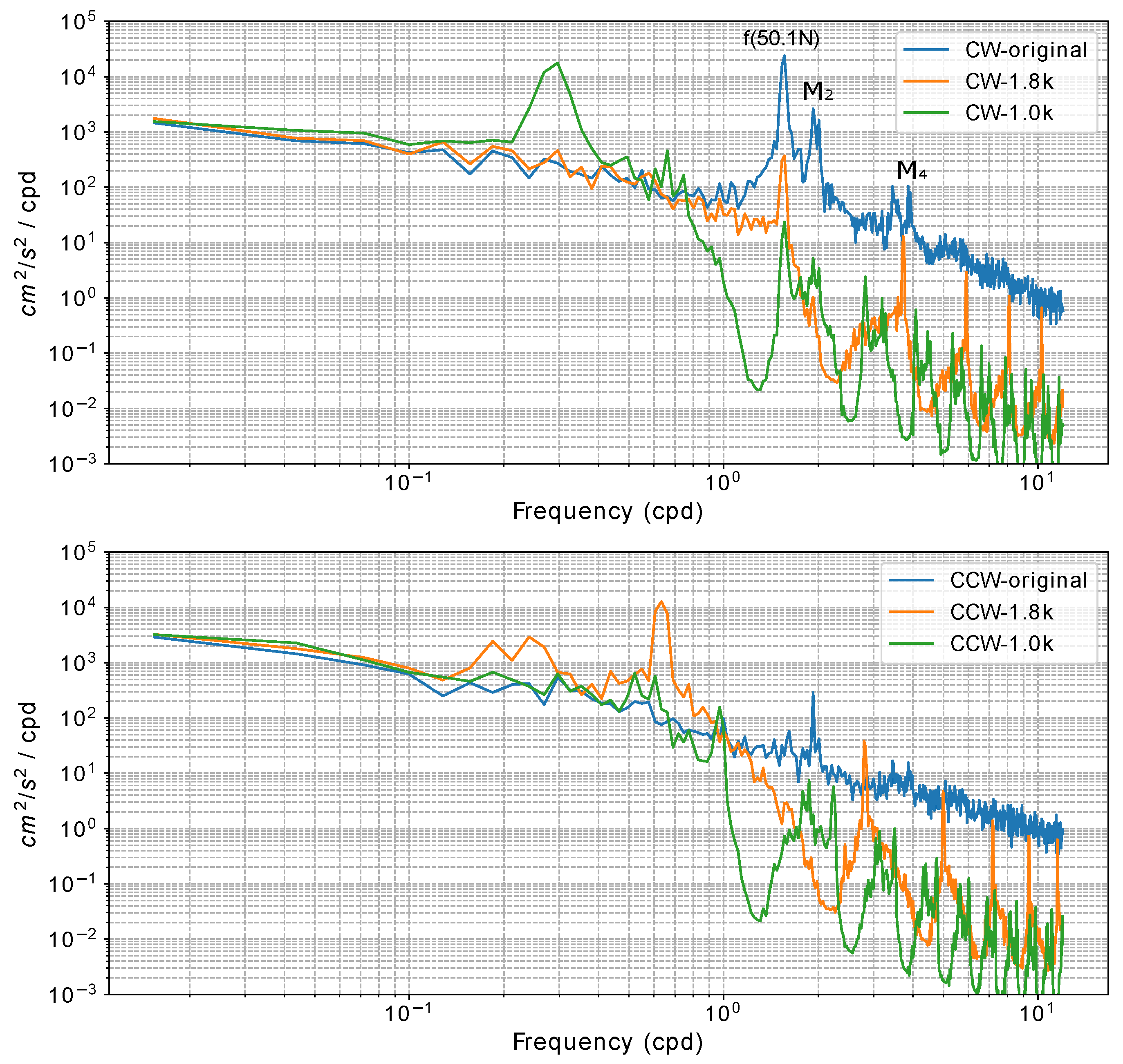
Figure 2 presents the rotary spectra of the observed surface velocities at station PAPA during the period from 8 June 2007, to 29 May 2008. The blue lines in the top panel represent the spectra obtained from the original hourly measurements. These spectra exhibit typical characteristics of surface velocity, with a dominant spectral peak observed at the inertial frequency, indicating downward propagation (Figure 2, top panel, Counter-clockwise CW component for the Northern Hemisphere). Furthermore, clear tidal peaks are observed at semi-diurnal frequencies.

To examine the aliasing effects resulting from different sampling methods, we present the spectra obtained from the ODYSEA sampling with two different swath sizes. The orange line corresponds to an 1800 km swath, denoted as CW-1.8 k, while the green line represents a 1000 km swath, denoted as CW-1.0 k. These spectra are generated by linearly interpolating the swath data onto an hourly temporal grid.

In the CW component, particularly for CW-1.0 k, the aliasing of the inertial frequency is prominently shown. This indicates that the chosen sampling interval is insufficient to accurately capture the full spectrum of the surface velocities. Conversely, in the CCW component, the 1.8 k swath exhibits aliasing of the M${}_2$ tide, resulting in a period of approximately 1.5 days. The observed rotary spectra provide insights into the surface velocity dynamics, showcasing the dominant inertial frequency and semi-diurnal tidal peaks. However, the aliasing effects from the different swath sizes, as demonstrated by the orange and green lines, highlight the limitations of the chosen sampling methods. These findings emphasize the need for careful consideration when selecting sampling intervals to avoid significant distortions in the spectral analysis of surface velocities and the need for a dynamical or statistical method to retrieve the high-frequency motions. More discussions about the aliasing are provided in Section 2.3.

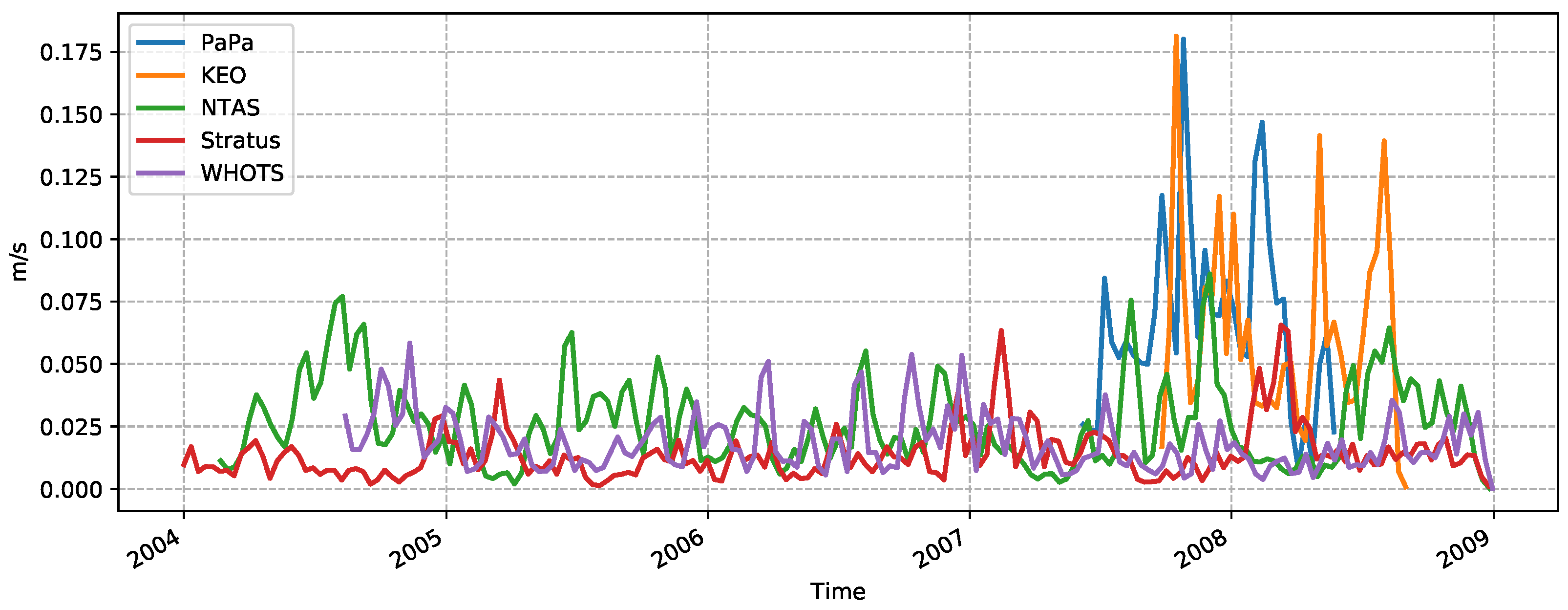
The time series of the NIO current velocity ($\sqrt{u^2+v^2}$) from the five stations is depicted in Figure 3. The mooring velocities are band-pass filtered around the local inertial frequency $f_0\pm 0.05f_0$ to extract the inertial velocity. At stations NTAS, Stratus, and WHOTS, NIOs have a magnitude of less than 5 cm/s, while this magnitude peaks at 18 cm/s at stations Papa and KEO. These magnitudes are consistent with those observed in the coupled simulation results.

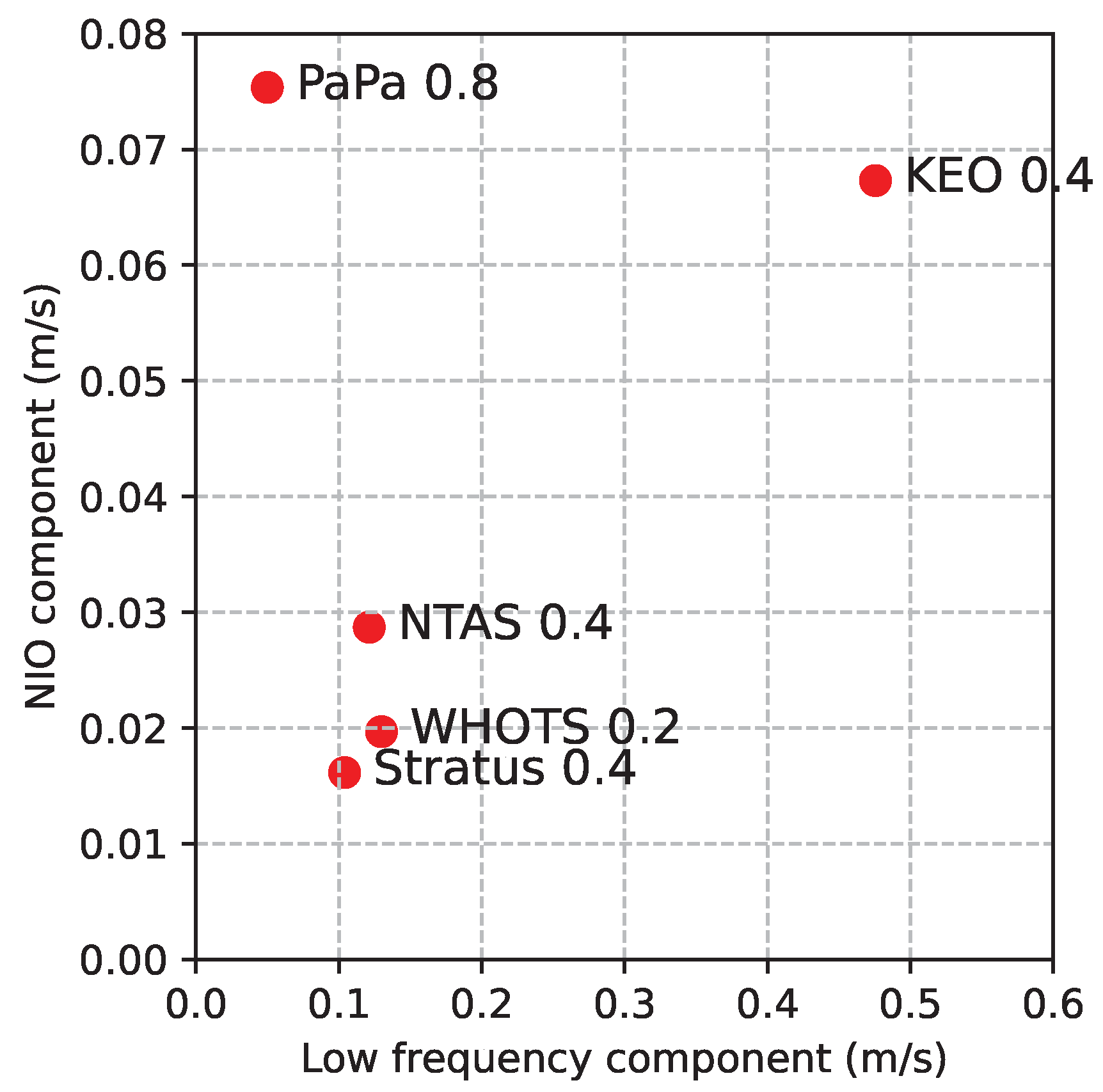
Figure 4 presents the kinetic energy contained in the inertial frequency and low frequency (periods larger than 4 days) at the five moorings, as determined through the use of low-pass and high-pass filters. The figure reveals that low-frequency—potentially balanced—motions dominate NIOs in amplitude. NIOs typically measure below 10 cm/s, while low-frequency motions typically exceed 10 cm/s. Station Papa is an exception, exhibiting an equal partition between NIOs and low-frequency motions. As it is located in an eddy desert in the northeastern Pacific, the NIO signal is prominent, making NIO reconstruction from ODYSEA observations relatively straightforward, as demonstrated later in Section 3.

On the other hand, KEO, situated in an atmospheric storm track region, features strong NIOs (10 cm/s) but much stronger low-frequency motions (50 cm/s) due to energetic western boundary currents and mesoscale eddies within. The ratio of NIO energy/variance to the total high-frequency motion energy (period < 4 days) is indicated by the number next to the mooring names in Figure 4. NIO accounts for 80 percent of the high-frequency variability at station Papa. As a result of this clear dominance, NIOs can be easily reconstructed at this station, even when undersampled by the narrower 1000 km swath (results shown in Section 3). At station KEO, however, 50 percent of high-frequency motions are not NIO, making it more challenging to reconstruct the NIO from the undersampled velocity. The NIO is less significant at stations NTAS, WHOTS, and Stratus. Consequently, we focus on further analyses at Papa and KEO, representing two distinct scenarios where NIO retrieval is either easy or more challenging, respectively.

2.2. The Coupled Ocean-Atmosphere Simulation (COAS)

The coupled ocean-atmosphere simulation used in this study is based on the Goddard Earth Observing System (GEOS) atmospheric and land models coupled with the ocean component of the Massachusetts Institute of Technology General Climate Model (MITgcm). The COAS configuration utilized in this research is thoroughly described in Strobach et al. [27], Torres et al. [8], and Torres et al. [11]. In brief, the atmospheric model has a nominal horizontal grid spacing of 1/16${}^{°}$ (approximately 6 km) with 72 vertical levels, and the ocean model features a nominal horizontal grid of 1/24${}^{°}$ (approximately 4 km) with 90 vertical levels. This nominal resolution is sufficient to resolve physical scales between 25 km and 30 km [8]. The frequent coupling between the ocean and atmosphere is also critical to capturing the correct NIO KE level.

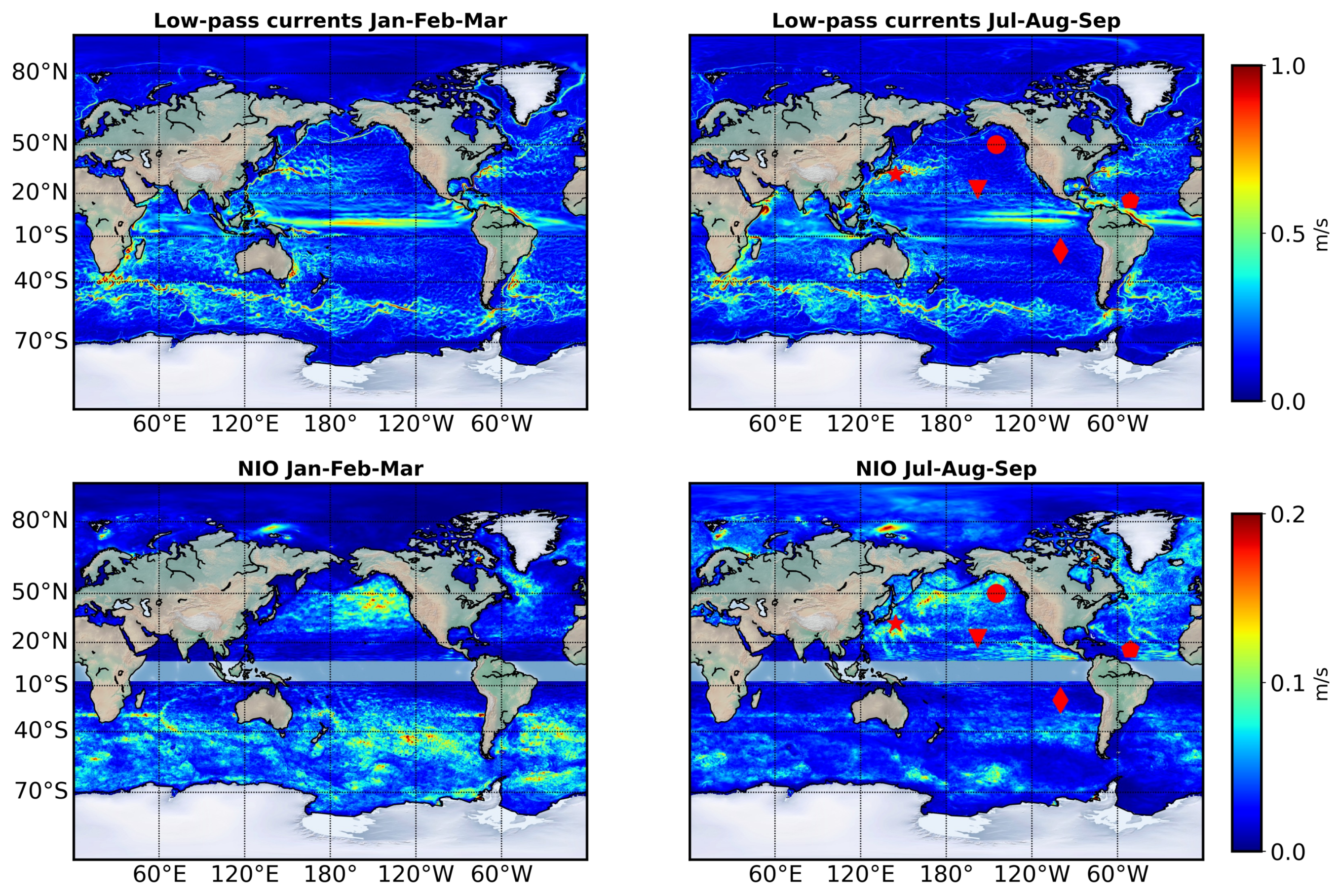
As shown in Figure 1, the low-pass surface currents (top panels), using a filter of 3 days, are considerably more energetic than band-pass NIO surface currents during both winter (January–February–March) and summer (July–August–September). The low-pass currents show values between 0.5–1.0 m/s in the western boundary currents, equatorial band, and in the Southern Ocean, while the amplitude for NIO is at most approximately 0.2 m/s. In fact, histograms demonstrate that 95% of NIO speeds are less than 0.1 m/s, with a median value of 0.02 m/s. However, a recent study [11], which combined COAS and the ODYSEA simulator, reported an underestimation of the wind energy input in the Northern Hemisphere during the summer. This underestimation can be attributed to the misrepresentation of NIO in ODYSEA observations, leading to a reduction in wind energy input at the NIO frequency band. It highlights the importance of a dynamical retrieval of NIO based on ODYSEA observations.

2.3. ODYSEA Sampling and the Slab Mixed-Layer Model

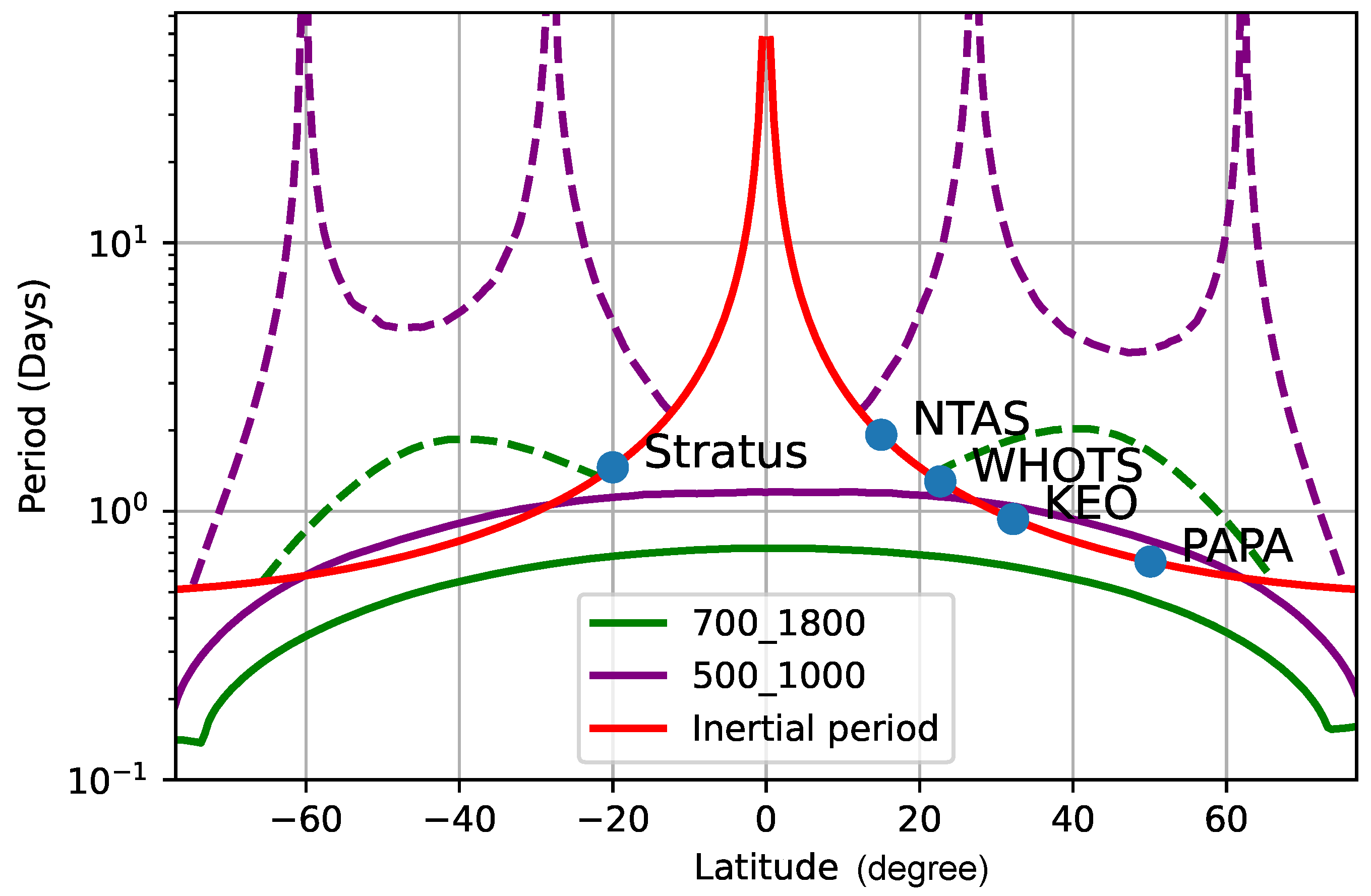
The sampling frequency of ODYSEA depends on the width of the swath. Figure 5 illustrates the average sampling period, $\Delta t$, as a function of latitude for two distinct orbits. The purple (green) solid lines represent swath widths of 1000 km (1800 km). The red line indicates the inertial period, $T=2\pi /f\left(\varphi \right)$, as a function of latitude, $\varphi$. The aliased periods are calculated following $T=2\pi /f_a=2\pi /|2*f_N-f\left(\varphi \right)|$, where $f_a$, $f_N$ represent the aliased frequency and Nyquist frequency ($\pi /\Delta t$), respectively.

The issue of aliasing is significant at mid-latitudes for both orbits. Aliasing is less severe at high latitudes due to the more frequent sampling provided by the wide swaths and at low latitudes due to longer inertial periods. Unfortunately, mid-latitudes, which are most affected by aliasing, also exhibit the most energetic NIOs due to energetic atmospheric storms.

The impact of aliasing is clearly demonstrated in the frequency spectra (Figure 2). The green and orange lines depict the rotary spectra of the simulated ODYSEA sampled surface velocities, sub-sampled from the hourly observations at station Papa (50.1${}^{°}$N, T = 15.64 h). The wider-swath scenario (1800 km) provides more frequency sampling at approximately 11.2-h intervals (orange lines). However, it does not capture most of the downward NIO (upper panel). The aliasing at this location occurs at $f_a=0.65$ cpd (1.55 days), intriguingly from the clockwise (CW) to the counter-clockwise (CCW) component. For the orbit with 1000 km swaths, severe aliasing occurs at $f_a=0.27$ cpd (3.7 days) for the CW component.

According to Pollard and Millard Jr [24], the inertial mixed layer currents can be represented by a damped slab model,

$$\begin{array}{ccc}\hfill \frac{du}{dt}-(f+\zeta /2)v& =& \frac{{\tau }_x}{H\rho }-ru,\hfill \end{array}$$

(1)

$$\begin{array}{ccc}\hfill \frac{dv}{dt}+(f+\zeta /2)u& =& \frac{{\tau }_y}{H\rho }-rv,\hfill \end{array}$$

(2)

with u and v the zonal and meridional velocities, ${\tau }_x$ and ${\tau }_y$ the zonal and meridional components of the wind stress, H the mixed layer depth, $\zeta$ the relative vorticity associated with mesoscale eddies, $\rho$ the density, and r a damping rate of NIOs. The frequency shift due to $\zeta$ is explained in Kunze [12]. For the forecast model used in this study, we simplified it to a linear slab model, which is used to predict NIO given an initial velocity, mixed layer depth, wind stress vector, and damping rate. The linear model is written as

$$\begin{array}{ccc}\hfill \frac{\partial u}{\partial t}-fv& =& \frac{{\tau }_x}{H\rho }-ru,\hfill \end{array}$$

(3)

$$\begin{array}{ccc}\hfill \frac{\partial v}{\partial t}+fu& =& \frac{{\tau }_y}{H\rho }-rv,\hfill \end{array}$$

(4)

We denote the forecast model as

$$\overrightarrow{u^f}=\mathcal{F}({\overrightarrow{u}}_0,\overrightarrow{\tau },H,r).$$

The hypothesis is that given the infrequent and possibly aliased wind stress and surface currents from ODYSEA, we can utilize the predictive power of the slab model constrained by the ODYSEA observations to reconstruct the NIO. This is an underdetermined problem that relies on optimizations for the best solution. We take the difference between the forecast slab model velocities and the ODYSEA observed velocities as the cost function of the optimization.

$$J({\overrightarrow{u}}_0,H,r)=\parallel \overrightarrow{u^f}\left(t_w\right)-{\overrightarrow{u}}_w\parallel ,$$

where $t_w$ is the time of the ODYSEA observations and $\overrightarrow{u^f}\left(t_w\right)$ is the slab model solution at $t_w$. An optimal set of control parameters $({\overrightarrow{u}}_0,H,r)$ is found by minimizing J.

In practice, the assumption of constant H may be validated for a short period. We conduct the optimization for a temporal window length of 10 inertial periods at mid-latitudes. This window length includes about 20 data points for each velocity component. The wind-stress is assumed to be given by ODYSEA and linearly interpolated between observations in the slab model integration. This certainly degrades the accuracy of the slab model prediction as the high-frequency (hourly winds) cannot be accurately captured by ODYSEA alone, but the winds can be compensated in reality, to some extent, by atmospheric reanalysis such as ERA5 [28].

3. Slab-Model Retrieval of NIO from ODYSEA, Results

3.1. Scenario One: Strong NIO in a Weak Eddy Regime

NIO is not only temporally intermittent but also has a strong geographic variation, as evidenced in Figure 1. In the first scenario, the NIO signal dominates high-frequency motions, and the background mesoscale variability is weak. Station Papa is a representative of this scenario (Figure 4). As one might expect, reconstructing NIO from ODYSEA should be relatively straightforward in this case due to the high signal-to-noise ratio, where ‘signal’ refers to NIO and ‘noise’ refers to high-frequency non-NIO motions.

Figure 6 illustrates the result of the slab-model reconstruction for Papa over a 10-day window. Gray lines, which are the same across all four panels, represent the true signal after a low-frequency sub-monthly component has been removed. The blue dots are simulated ODYSEA observations with (lower panels) and without (upper panels) noise and errors. The true NIO (green lines) is derived by applying a Butterworth bandpass filter to the truth (gray lines). The red line in each panel represents the slab-model NIO prediction based on the ODYSEA observations in each scenario. The left panels show the case with a 1000 km swath, while the right panels display the results of an 1800 km swath. The aliasing effect is particularly clear in this case, as the signal itself is dominated by the periodic NIO. The blue lines exhibit aliased oscillations at lower frequencies. The 1000 km swath sampling (Figure 6 upper left) displays an oscillation at a near 4-day period, which is consistent with the calculations in Section 2.3, while the 1800 km swath sampling presents a regular oscillation at about 1.7 days. The linear interpolation (blue lines) does not capture the local NIO but instead produces aliased oscillations, as expected.

Conversely, the slab model uses the sparsely sampled velocities as a constraint to enforce oscillations at the inertial frequency. The results in this case demonstrate a high level of skill in retrieving the missing information. The red curves represent the slab-model retrieval and compare well with the true NIO (green lines), even for cases with 10 cm/s ODYSEA observational errors (lower panels). The RMS difference between the filtered NIO and the slab-model reconstructed NIO is below 2 cm/s. The high performance of the slab model at Station Papa is consistent throughout the entire year (Figure 7, upper panel). The slab-model reconstruction (orange line) matches well with the true NIO (blue curve) (bandpass-filtered ocean currents).

Wind Work at Inertial Frequency by ODYSEA

The intermittent winds drive most of the mixed layer NIOs and contribute to the subsequent energy dissipation at the base of the mixed layer as well as the deep ocean. Using the damped slab model (Equation (1)), the mixed layer kinetic energy equation can be written as

$$\frac{\mathrm{d}}{\mathrm{d}t}{\mathrm{KE}}_I={\mathrm{\Pi }}_W+{\mathrm{\Pi }}_H+{\mathrm{\Pi }}_R,$$

(5)

where ${\mathrm{KE}}_I=0.5\rho H{\left|\mathbf{u}\right|}^2$ is the mixed layer inertial kinetic energy, ${\mathrm{\Pi }}_W$ the wind work, ${\mathrm{\Pi }}_H=0.5\rho {\left|\mathbf{u}\right|}^2\frac{\mathrm{d}H}{\mathrm{d}t}$ the energy flux of changing the mixed layer depth H, and ${\mathrm{\Pi }}_R$ encompasses all the energy sinks due to dissipation and downward energy radiation that remove kinetic energy from the mixed layer and are often parameterized. Here we demonstrate that with the current NIO retrieval, we can at least retrieve the wind work ${\mathrm{\Pi }}_W$.

With observed winds and ocean surface currents, we may be able to retrieve the high-frequency wind work at inertial frequency. The slab model reconstructs high-frequency ocean motions. The diagnosed wind work is shown in the bottom panel of Figure 7. In the slab model results (orange line), the ocean currents are reconstructed using the slab model, and the atmospheric winds are the linear interpolation of ODYSEA observations. The truth (blue line) represents the wind work of the true observed (bandpass-filtered) ocean currents and the hourly winds. The reconstructed wind work accounts for more than 90 percent of the truth.

Existing observations and atmospheric reanalysis do not contain sufficient high-frequency information for a global budget estimate [8]. ODYSEA can potentially solve the problem if the NIO can be accurately reconstructed. The results for Papa clearly demonstrated the first scenario, where NIO is strong and eddies are weak. In this scenario, NIO reconstruction can be completed accurately even for a narrower swath (1000 km) with well below 10 cm/s observational error. In the next section, we will use the data from KEO to test scenario two, where both low-frequency (presumably balanced motions) and high-frequency (periods less than 3 days) are strong. In this scenario, NIO can become ambiguous due to the high-frequency variability caused by submesoscale dynamics with periods of days or less.

3.2. Scenario Two: Strong NIO in a Strong Mesoscale Eddy Regime

In the KEO region, both NIOs and mesoscale eddies exhibit high variability, with the mesoscale kinetic energy about 25 times larger than the NIO kinetic energy (refer to Figure 4). The low-frequency component can be retrieved by low-pass filtering the ODYSEA observations, but the high-frequency eddies impose challenges in the slab model NIO reconstruction.

Figure 8 demonstrates an instance of a 10-day window slab model reconstruction in this region. For comparison, we have also included results based on harmonic fitting (green curve) and the total high-frequency (less than 4 days) velocity (dashed curves). The left panels display results based on the 1000 km swath. The slab model and harmonic analysis do not provide an accurate NIO reconstruction, even without ODYSEA measurement error (top left panel). This is largely due to the large temporal gaps, which are exacerbated by high-frequency non-NIO signals. With a 10 cm/s instrument noise (bottom left panel), the reconstructions (blue and green lines) become less relevant to the real NIO (black line). However, the reconstruction’s accuracy is significantly improved with a wider swath (1800 km), which effectively increases the sampling frequency (Figure 2). The slab model and harmonic analysis can retrieve NIO with the correct amplitude and phase (top right panel, Figure 8), even with ‘contamination’ from high-frequency non-NIO signals. Even with 10 cm/s noise, the slab model can still reconstruct the NIO with the correct phase and slightly degraded amplitude (bottom right panel). The error RMS is below 5 cm/s. However, the harmonic analysis in this case exhibits a much larger difference in amplitude, although it still retains the correct phase (green curve). These results strongly underscore the relevance of using an 1800 km-wide swath instead of a 1000 km-wide swath.

4. Discussions

To summarize, we have established a viable approach for utilizing a linearized slab mixed-layer model to infer near-inertial oscillations from an envisioned satellite mission, ODYSEA, tasked with simultaneous observations of wind and currents [8,22]. While the preliminary results are promising and consistent with previous similar analyses [29], there are several avenues for further refinement.

Expanding the observation swath confers several benefits. Not only does it enhance the temporal sampling frequency, but it also delivers an instantaneous two-dimensional snapshot of surface velocity fields. The exploitation of a wider swath, for instance, through spatial filtering prior to fitting the slab model, could notably augment the accuracy of NIO reconstructions, especially in complex regions such as KEO, where submesoscale eddies make substantial contributions to high-frequency motions. COAS analysis indicates that NIOs predominantly exhibit larger spatial scales than those of mesoscale and submesoscale structures. We anticipate expanding this study with a comprehensive analysis based on COAS outputs.

In the current version, our slab model does not consider background vorticity. Considering background velocity shear directly derived from ODYSEA observations in the optimization process can potentially increase the accuracy of the slab-model reconstruction. Additionally, incorporating a time-varying mixed layer depth could lead to a more realistic reconstruction of mixed layer dynamics and potentially improve the optimization results. The mixed-layer depth is also known to be impacted by mesoscale eddies and can potentially be represented by parameterization, such as the one proposed in [30].

The wind data used in our optimizations is directly sourced from ODYSEA’s simultaneous sampling and linearly interpolated between observations (about 12 hourly). A more precise retrieval of NIOs might be achieved if we incorporated higher-frequency wind data, such as those produced by ERA5. Alternatively, for a better scenario, missing high-frequency winds between two consecutive ODYSEA observations could be treated as a control parameter and estimated within the same optimization framework.

With these improvements, we will be effectively conducting a data assimilation procedure based on the slab model (Equation (1)), enabling us to estimate NIO velocity, mixed layer depth, high-frequency winds, and consequently the mixed layer kinetic energy budget. These potential improvements form the basis of our future work.

5. Conclusions

Results from this study demonstrate the feasibility of retrieving wind-forced NIOs from ODYSEA observations and, therefore, diagnosing the wind energy input to NIO. This can be achieved using a calibrated slab mixed-layer model. We considered two distinct scenarios. The first one concerns highly energetic NIOs and weakly energetic mesoscale eddies. Retrieving NIO in this scenario is relatively easy. The second scenario concerns energetic NIOs and energetic mesoscale eddies. In this scenario, the diagnosis of NIOs is less accurate but can still be kept within a 10 cm/s error. Our results show that NIOs can be recovered with such accuracy using the ODYSEA spatial and temporal resolution, but only if observations are made in a wide swath of 1800 km. A narrower, wider swath (1000 km) leads to stronger aliasing.

However, potential improvements can be made by fully utilizing the wide-swath ODYSEA observations beyond the increased temporal resolution. The improvements include considering spatial filtering of wide-swath surface currents before optimization, the vorticity from the background circulation and mesoscale eddies, varying mixed layer depth, and including high-frequency winds in the optimization process. These improvements will be studied using high-resolution coupled simulation in the future.

References

1. Gill, A.E. Atmosphere. Ocean. Dyn. 1982, 30, 662. [Google Scholar]
2. Klein, P.; Coantic, M. A numerical study of turbulent processes in the marine upper layers. J. Phys. Oceanogr. 1981, 11, 849–863. [Google Scholar] [CrossRef]
3. Large, W.; Crawford, G. Observations and simulations of upper-ocean response to wind events during the ocean storms experiment. J. Phys. Oceanogr. 1995, 25, 2831–2852. [Google Scholar] [CrossRef]
4. Skyllingstad, E.D.; Smyth, W.; Crawford, G. Resonant wind-driven mixing in the ocean boundary layer. J. Phys. Oceanogr. 2000, 30, 1866–1890. [Google Scholar] [CrossRef]
5. Klein, P.; Lapeyre, G.; Large, W. Wind ringing of the ocean in presence of mesoscale eddies. Geophys. Res. Lett. 2004, 31, L15306. [Google Scholar] [CrossRef]
6. Rimac, A.; von Storch, J.S.; Eden, C.; Haak, H. The influence of high-resolution wind stress field on the power input to near-inertial motions in the ocean. Geophys. Res. Lett. 2013, 40, 4882–4886. [Google Scholar] [CrossRef]
7. Yu, Z.; Fan, Y.; Metzger, E.J.; Smedstad, O.M. The wind work input into the global ocean revealed by a 17-year global HYbrid coordinate ocean model reanalysis. Ocean. Model. 2018, 130, 29–39. [Google Scholar] [CrossRef]
8. Torres, H.S.; Klein, P.; Wang, J.; Wineteer, A.; Qiu, B.; Thompson, A.F.; Rodriguez, E.; Menemenlis, D.; Molod, A.; Hill, C.N.; et al. Wind work at the air-sea interface: A Modeling Study in Anticipation of Future Space Missions. Geosci. Model Dev. 2022, 15, 8041–8058. [Google Scholar] [CrossRef]
9. Ferrari, R.; Wunsch, C. Ocean circulation kinetic energy: Reservoirs, sources, and sinks. Annu. Rev. Fluid Mech. 2009, 41, 253–282. [Google Scholar] [CrossRef]
10. Liu, Y.; Jing, Z.; Wu, L. Wind power on oceanic near-inertial oscillations in the global ocean estimated from surface drifters. Geophys. Res. Lett. 2019, 46, 2647–2653. [Google Scholar] [CrossRef]
11. Torres, H.; Wineteer, A.; Klein, P.; Lee, T.; Wang, J.; Rodriguez, E.; Menemenlis, D.; Zhang, H. Anticipated Capabilities of the ODYSEA Wind and Current Mission Concept to Estimate Wind Work at the Air&ndash;Sea Interface. Remote Sens. 2023, 15, 3337. [Google Scholar] [CrossRef]
12. Kunze, E. Near-inertial wave propagation in geostrophic shear. J. Phys. Oceanogr. 1985, 15, 544–565. [Google Scholar] [CrossRef]
13. Young, W.; Jelloul, M.B. Propagation of near-inertial oscillations through a geostrophic flow. J. Mar. Res. 1997, 55, 735–766. [Google Scholar] [CrossRef]
14. Danioux, E.; Klein, P.; Rivière, P. Propagation of wind energy into the deep ocean through a fully turbulent mesoscale eddy field. J. Phys. Oceanogr. 2008, 38, 2224–2241. [Google Scholar] [CrossRef]
15. Furuichi, N.; Hibiya, T.; Niwa, Y. Model-predicted distribution of wind-induced internal wave energy in the world’s oceans. J. Geophys. Res. Ocean. 2008, 113, C09034. [Google Scholar] [CrossRef]
16. Danioux, E.; Klein, P.; Hecht, M.W.; Komori, N.; Roullet, G.; Le Gentil, S. Emergence of wind-driven near-inertial waves in the deep ocean triggered by small-scale eddy vorticity structures. J. Phys. Oceanogr. 2011, 41, 1297–1307. [Google Scholar] [CrossRef]
17. Joyce, T.M.; Toole, J.M.; Klein, P.; Thomas, L.N. A near-inertial mode observed within a Gulf Stream warm-core ring. J. Geophys. Res. Ocean. 2013, 118, 1797–1806. [Google Scholar] [CrossRef]
18. Barkan, R.; Winters, K.B.; McWilliams, J.C. Stimulated imbalance and the enhancement of eddy kinetic energy dissipation by internal waves. J. Phys. Oceanogr. 2017, 47, 181–198. [Google Scholar] [CrossRef]
19. Flexas, M.M.; Thompson, A.F.; Torres, H.S.; Klein, P.; Farrar, J.T.; Zhang, H.; Menemenlis, D. Global Estimates of the Energy Transfer From the Wind to the Ocean, With Emphasis on Near-Inertial Oscillations. J. Geophys. Res. Ocean. 2019, 124, 5723–5746. [Google Scholar] [CrossRef]
20. Rodríguez, E.; Wineteer, A.; Perkovic-Martin, D.; Gál, T.; Stiles, B.W.; Niamsuwan, N.; Rodriguez Monje, R. Estimating ocean vector winds and currents using a Ka-band pencil-beam Doppler scatterometer. Remote Sens. 2018, 10, 576. [Google Scholar] [CrossRef]
21. Rodríguez, E.; Bourassa, M.; Chelton, D.; Farrar, J.T.; Long, D.; Perkovic-Martin, D.; Samelson, R. The winds and currents mission concept. Front. Mar. Sci. 2019, 6, 438. [Google Scholar] [CrossRef]
22. Wineteer, A.; Perkovic-Martin, D.; Monje, R.; Rodríguez, E.; Gál, T.; Niamsuwan, N.; Nicaise, F.; Srinivasan, K.; Baldi, C.; Majurec, N.; et al. Measuring winds and currents with Ka-band doppler scatterometry: An airborne implementation and progress towards a spaceborne mission. Remote Sens. 2020, 12, 1021. [Google Scholar] [CrossRef]
23. Wineteer, A.; Torres, H.S.; Rodriguez, E. On the Surface Current Measurement Capabilities of Spaceborne Doppler Scatterometry. Geophys. Res. Lett. 2020, 47, e2020GL090116. [Google Scholar] [CrossRef]
24. Pollard, R.T.; Millard, R., Jr. Comparison between observed and simulated wind-generated inertial oscillations. Deep-Sea Res. 1970, 17, 813–821. [Google Scholar] [CrossRef]
25. D’Asaro, E.A. The energy flux from the wind to near-inertial motions in the surface mixed layer. J. Phys. Oceanogr. 1985, 15, 1043–1059. [Google Scholar] [CrossRef]
26. Alford, M.H.; MacKinnon, J.A.; Simmons, H.L.; Nash, J.D. Near-inertial internal gravity waves in the ocean. Annu. Rev. Mar. Sci. 2016, 8, 95–123. [Google Scholar] [CrossRef]
27. Strobach, E.; Klein, P.; Molod, A.; Fahad, A.A.; Trayanov, A.; Menemenlis, D.; Torres, H. Local Air-Sea Interactions at Ocean Mesoscale in Western Boundary Currents. Geophys. Res. Lett. 2022, 49, e2021GL097003. [Google Scholar] [CrossRef]
28. Hersbach, H.; Bell, B.; Berrisford, P.; Hirahara, S.; Horányi, A.; Muñoz-Sabater, J.; Nicolas, J.; Peubey, C.; Radu, R.; Schepers, D.; et al. The ERA5 global reanalysis. Q. J. R. Meteorol. Soc. 2020, 146, 1999–2049. [Google Scholar] [CrossRef]
29. Ubelmann, C.; Dibarboure, G.; Gaultier, L.; Ponte, A.; Ardhuin, F.; Ballarotta, M.; Faugère, Y. Reconstructing ocean surface current combining altimetry and future spaceborne Doppler data. J. Geophys. Res. Ocean. 2021, 126, e2020JC016560. [Google Scholar] [CrossRef]
30. Klein, P.; Hua, B.L. The mesoscale variability of the sea surface temperature: An analytical and numerical model. J. Mar. Res. 1990, 48, 729–763. [Google Scholar] [CrossRef]
Figure 1. The low-pass filtered (periods larger than 3 days) surface velocity from the coupled simulation (top panel, described in Section 2) and the band-pass filtered (bandwidth frequency [0.95f, 1.05f]) near inertial velocity (lower panel) for January-Feburary-March (left panels) and July-August-September (right panels). Note that the color scale is divided by 5 in the bottom panels. The coupled simulation has a nominal 4 km resolution in the ocean and 6 km in the atmosphere [8,11]. The five mooring locations are shown by the symbols in the right panels.
Remotesensing 15 04526 g001
Figure 2. The rotary spectrum of the station PAPA surface velocities for the period 8 June 2007–29 May 2008. The upper and lower panels correspond to the Clockwise (CW) and Counter-Clockwise (CCW) components, respectively. The blue lines are the spectra of the original hourly measurements from observations. The orange (green) lines represent the spectra from the ODYSEA sampling with a 1800 km (1000 km) swath linearly interpolated on to an hourly temporal grid (denoted as CW-1.8 k and CW-1.0 k, respectively). The aliasing of the inertial frequency is clearly shown in CW component, especially for CW-1.0 k. The 1.8 k swath aliased M2 tide into approximately 1.5-day period in the CCW component. The spectrum slope is -2.2 and -1 for the CW and CCW component, respectively, consistent with previous observations [26] indicating the dominance of energy in the downward component.
Remotesensing 15 04526 g002
Figure 3. The time series of the NIO currents averaged over a 10-day boxcar sliding window from the five stations.
Remotesensing 15 04526 g003
Figure 4. This figure highlights the distribution of currents in the global ocean. The hourly time series of the surface velocity was separated into low and high-frequency components using a high-pass Butterworth filter with a cutoff period of 4 days. The NIO was bandpass-filtered between f 0 ± 0.05 f 0 . The observed current velocity at the five stations is plotted on low-frequency (x-axis) and NIO-velocity (y-axis) coordinates. The numbers next to the label are the ratio between NIO-kinetic energy and total high-frequency motion kinetic energy.
Remotesensing 15 04526 g004
Figure 5. The inertial period T = 2 π / f ( ϕ ) as a function of latitude ϕ with a unit of days (red line). The sampling periods of ODYSEA ( Δ t ) with 1800 km and 1000 km swaths are shown in green and purple, respectively. The first aliasing period of the two orbits are shown in dashed lines calculated from f a = | 2 * f N f ( ϕ ) | , where f a , f N are the aliased frequency and Nyquist frequency ( π / Δ t ), respectively. The names of the five stations are denoted at their corresponding latitudes on the line of the inertial period (red).
Remotesensing 15 04526 g005
Figure 6. An example of the slab model reconstruction (red curves) of the NIO based on simulated ODYSEA observations (blue dots) for the 1k-km swath (left) and 1.8 k-km swath (right) using the station Papa observations is shown. The upper panels display the results without noise, while the lower panels incorporate the influence of random observational errors in surface currents, with a Gaussian error of 10 cm/s RMS. Only zonal velocity is plotted in this illustration. The gray curves represent the observed velocity high-pass filtered with a cutoff period of 30 days. The low-frequency component is removed from both ODYSEA (dots) and truth (gray curves). The green curives represents the true NIO derived from the gray curve using a bandpass Butterworth filter within the frequency band [ 0.95 f , 1.05 f ] .
Remotesensing 15 04526 g006
Figure 7. For swath 1800km, no noise, ODYSEA wind, The 6-day average of the NIO current speed | U I | (upper) and the near-inertial wind work τ · u (lower).
Remotesensing 15 04526 g007
Figure 8. The result of NIO reconstruction based on the KEO mooring. Left panels (a,c) show the result with a 1000-km swath. Right panels (b,d) are for an 1800-km swath. The top panels (a,b) are based on truth observations. The bottom panels (c,d) display results with a 0.1 m/s noise added to ODYSEA observations. The highpass-filtered hourly observations are shown as a dashed-gray curve. The black curve represents the bandpass-filtered truth NIO signal, which is consistent across all four panels. The green curve represents the Harmonic reconstruction. The blue curve displays the slab model reconstruction. The orange dots are the ODYSEA observations.
Remotesensing 15 04526 g008