
Evaluation of Simulated CO2 Point Source Plumes from High-Resolution Atmospheric Transport Model
 , ,
, ,
Abstract
:1. Introduction
2. The Lagrangian Particle Dispersion Model
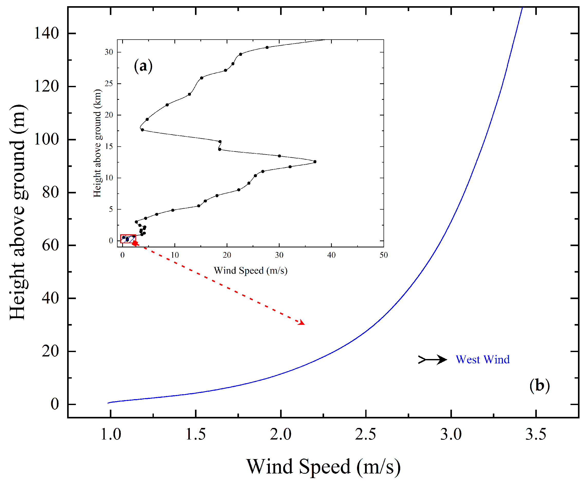
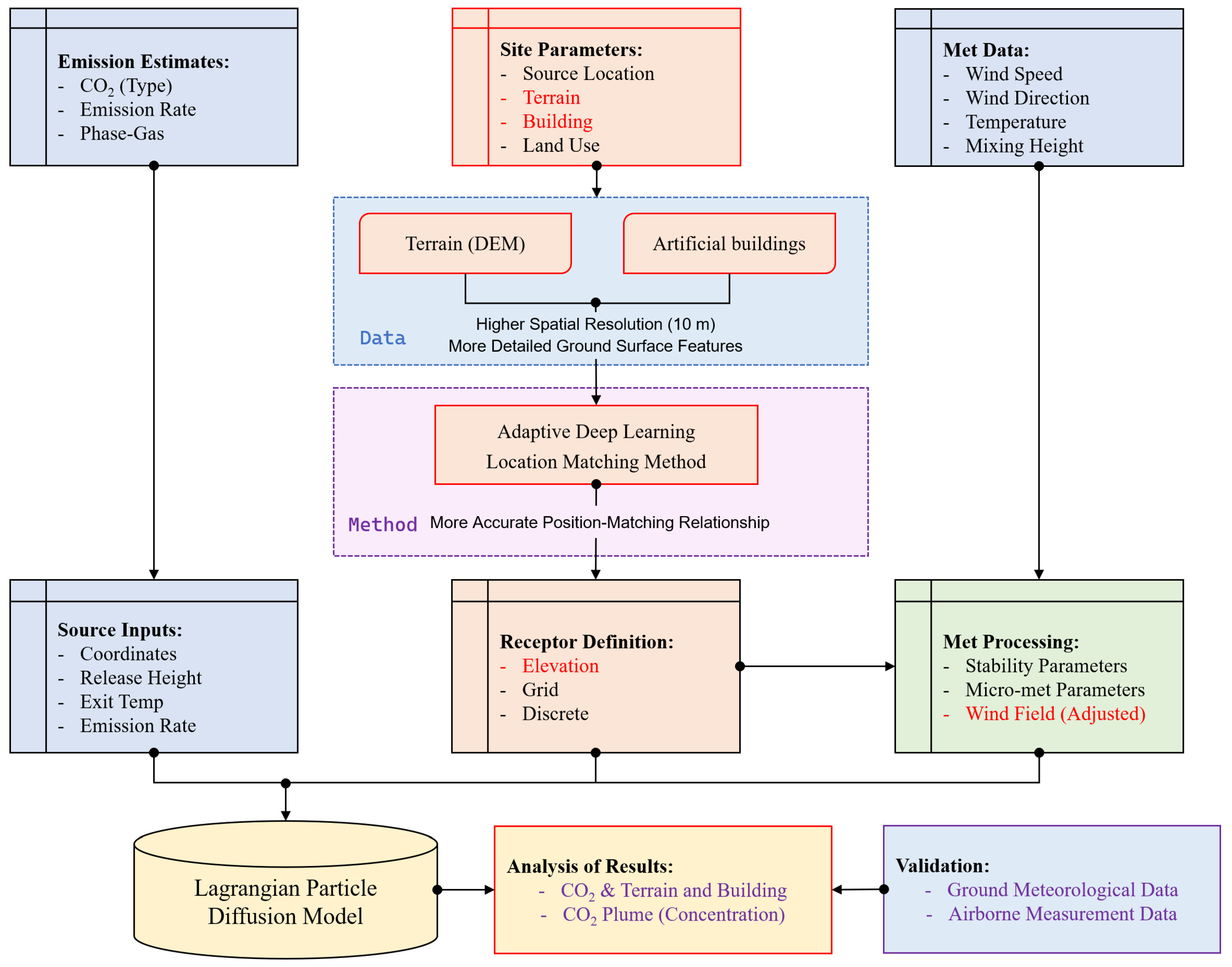
- Adjusting the wind field based on large-scale terrain.
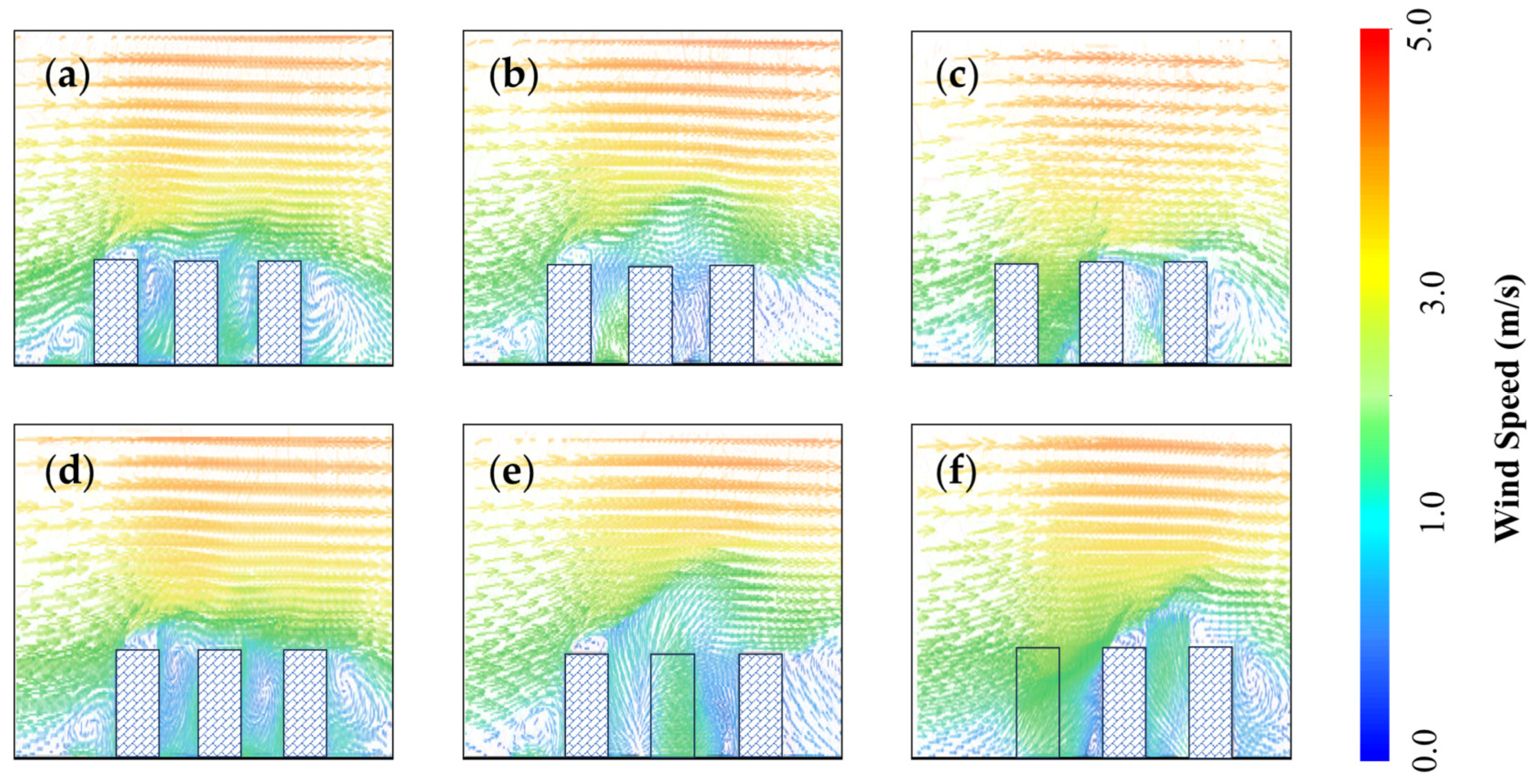
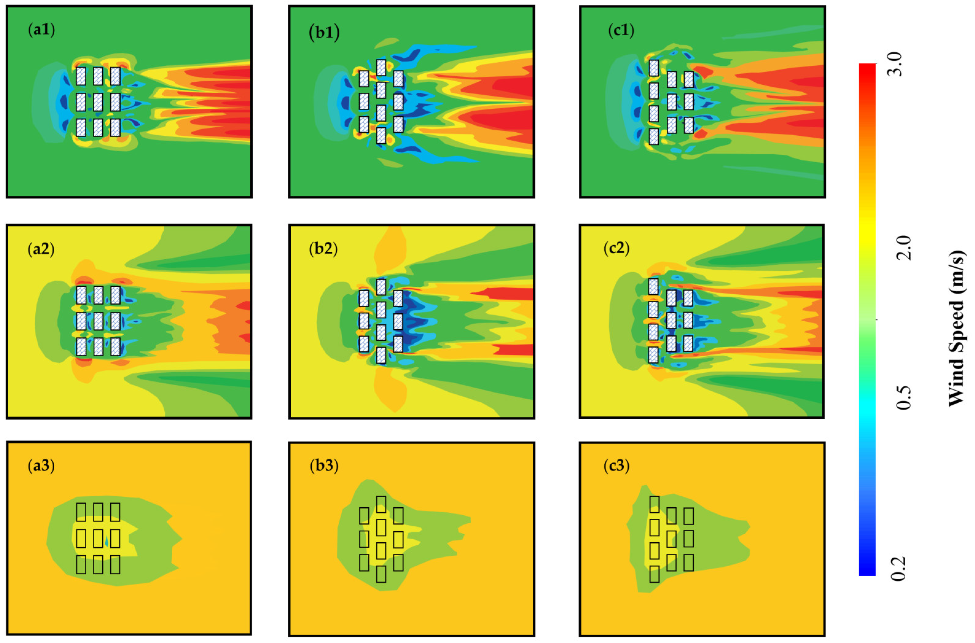
- Precisely simulating the interaction between CO2 plume and terrain under conditions where the large-scale wind field has minimal impact.
- Simplifying the interaction between CO2 plume and terrain (including both large and small-scale terrain features). This involves employing streamline-layering estimation for plume deviation caused by complex subgrid-scale terrain, using plume trajectory coefficient adjustment method and stress-adjustment method to simplify parameter adjustments for plume height changes due to terrain, plume collision with mountains, and the effect of increased diffusion coefficients.
3. Sensitivity Analysis of Surface Characteristics for CO2 Dispersion
4. Data Selection and Processing
4.1. Data Selection
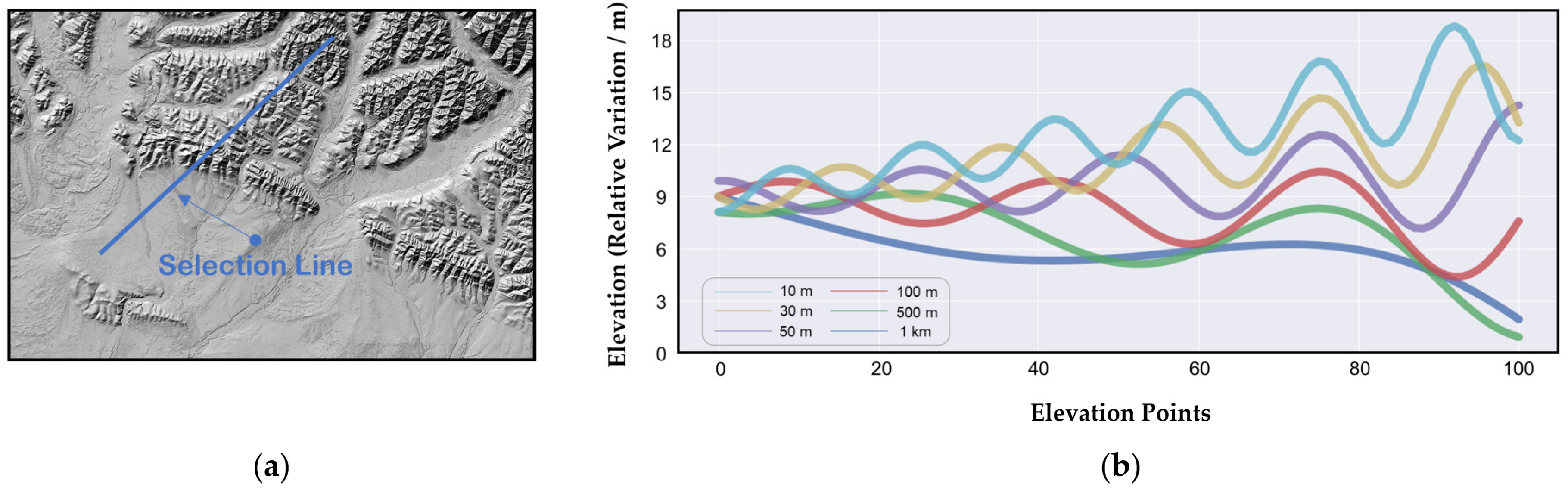
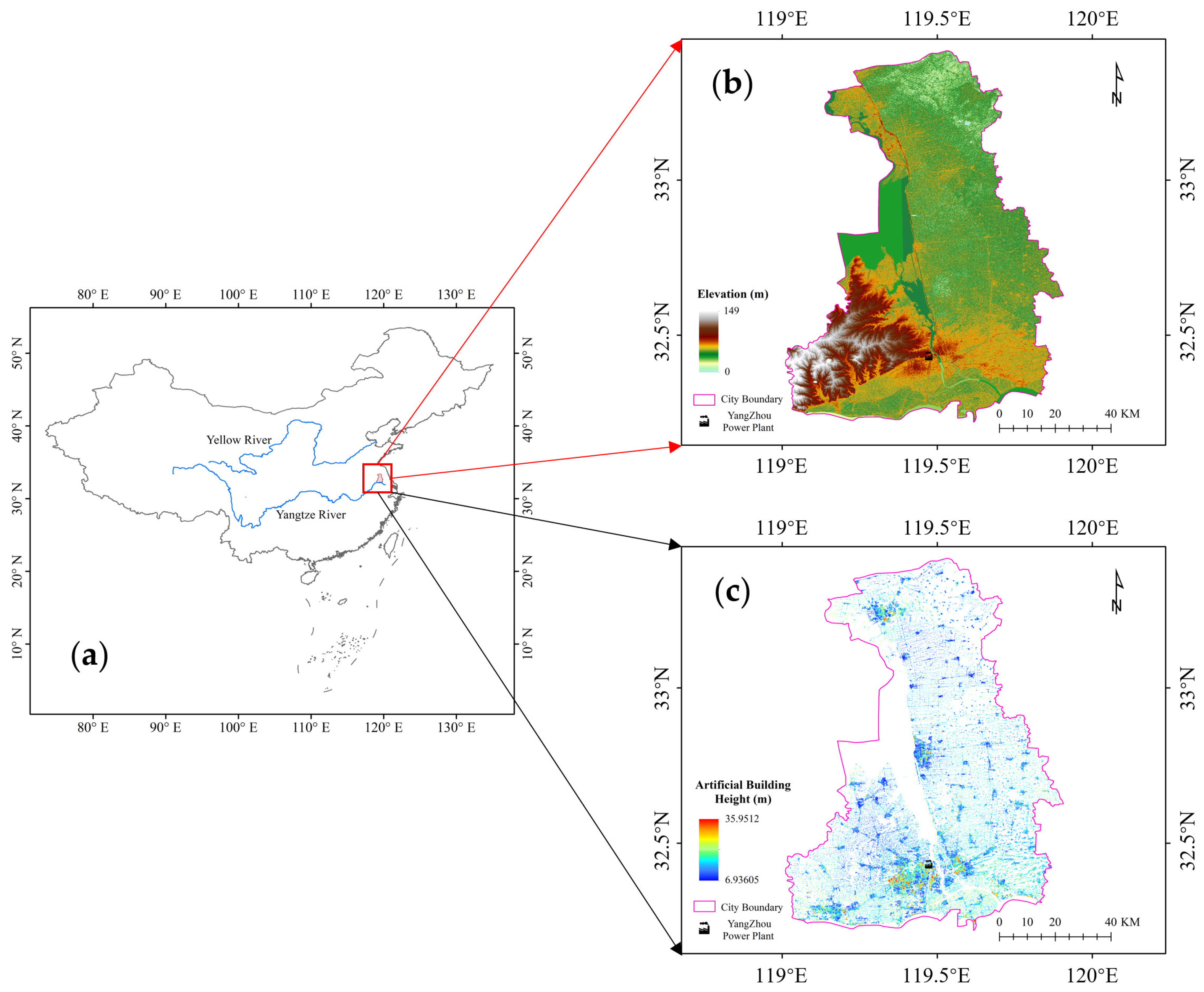
4.1.1. DEM
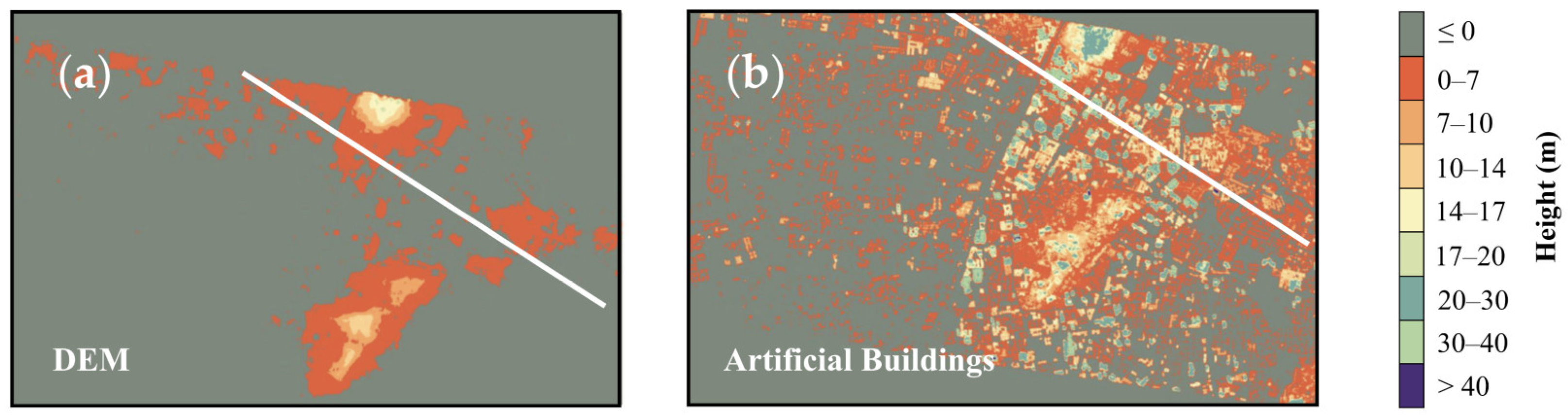
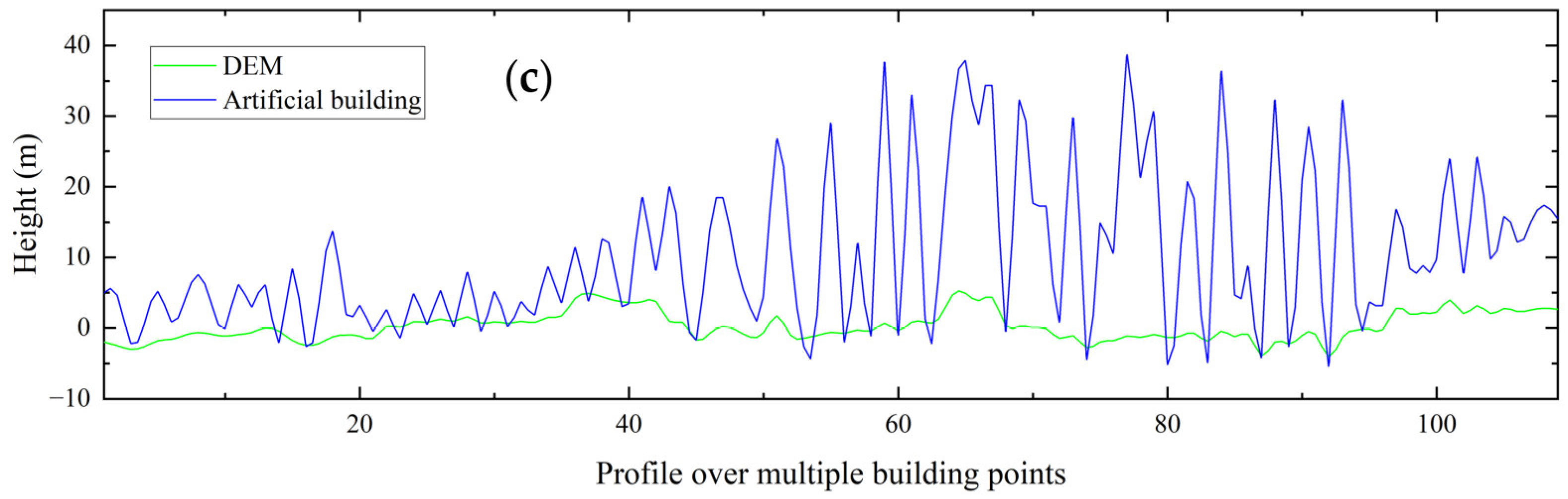
4.1.2. Artificial Buildings
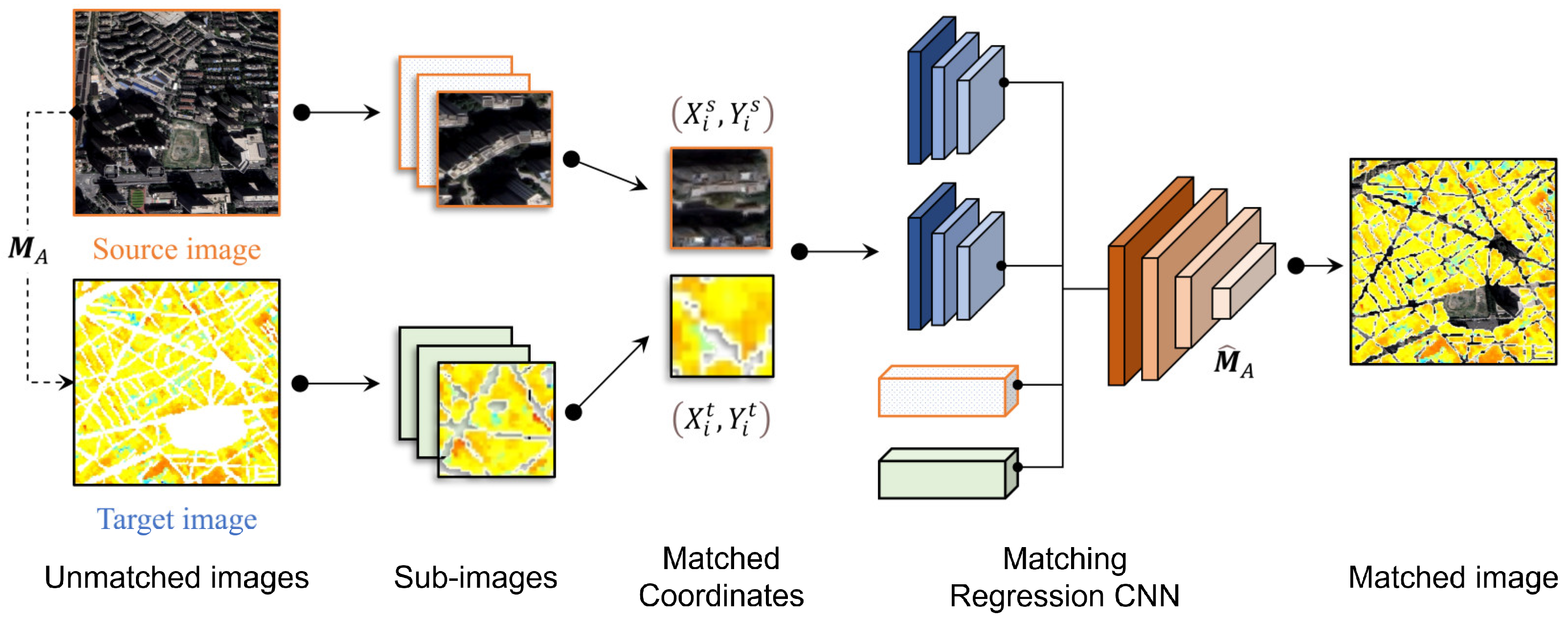
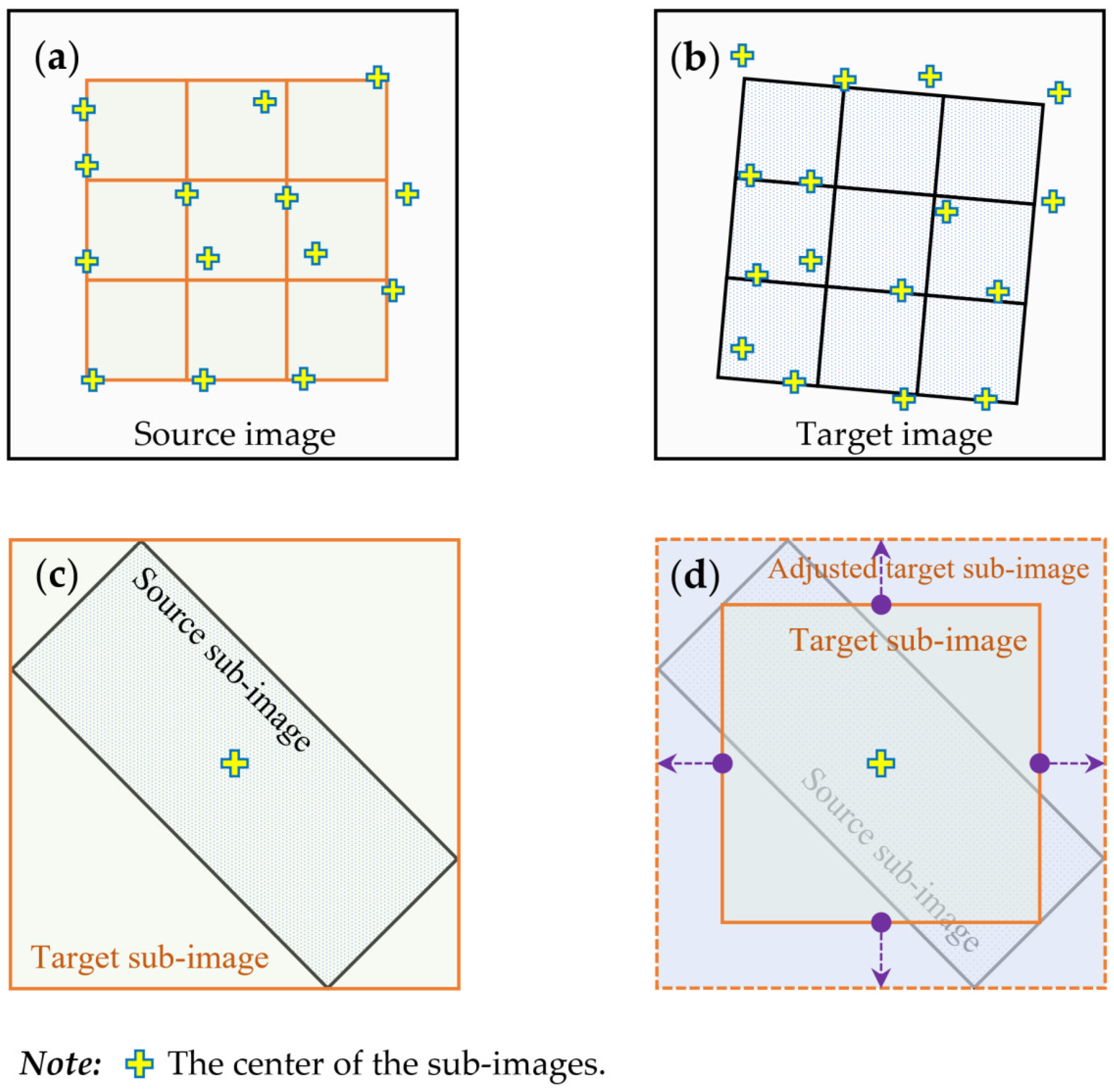
4.2. Adaptive Deep Learning Location Matching Method
4.2.1. Method Construct
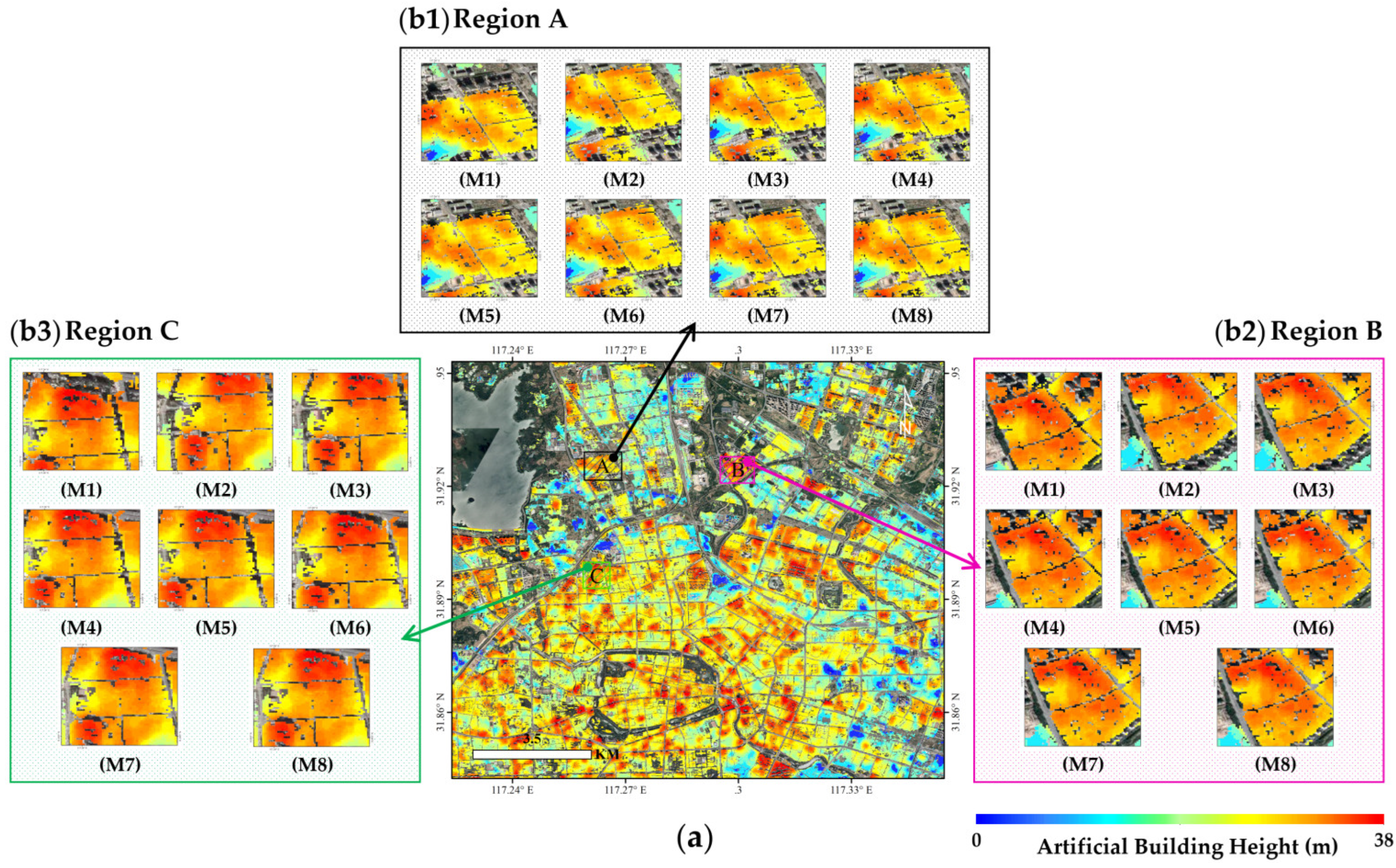
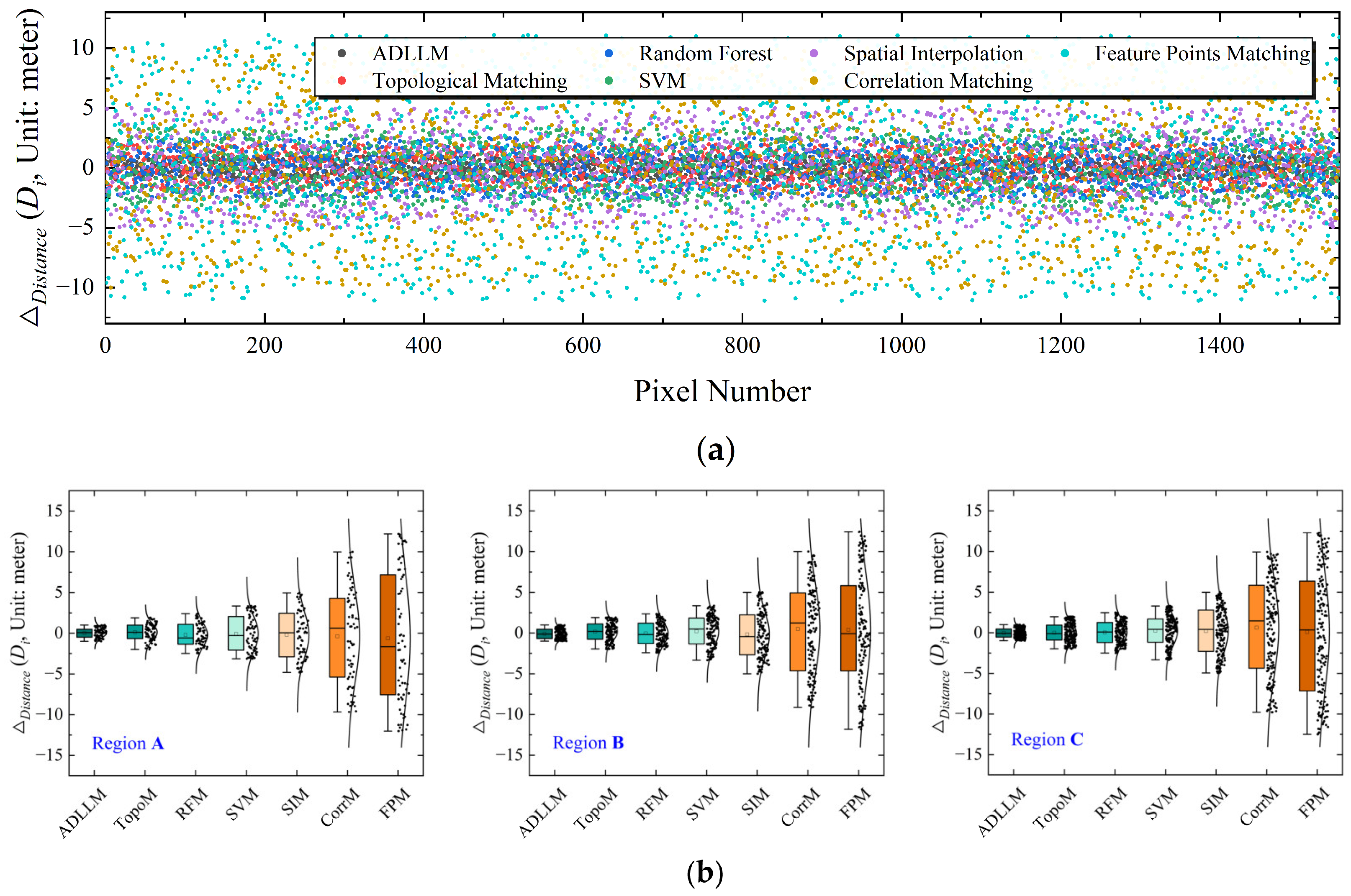
4.2.2. Position Matching Accuracy Evaluation
5. Aircraft Measurement Validation
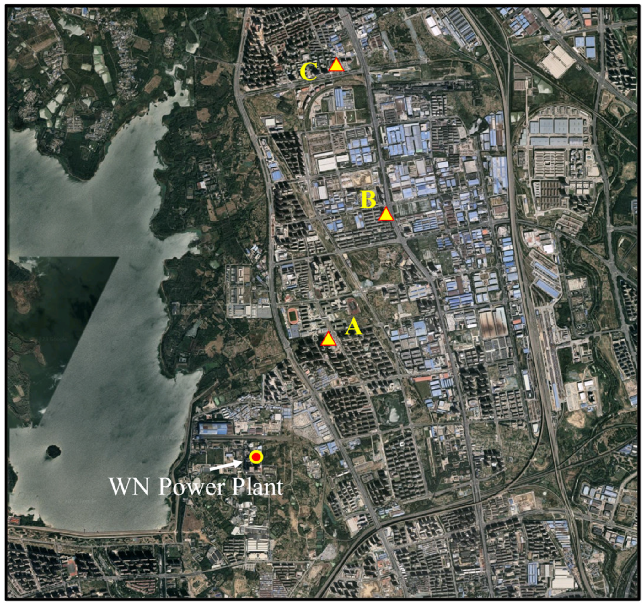
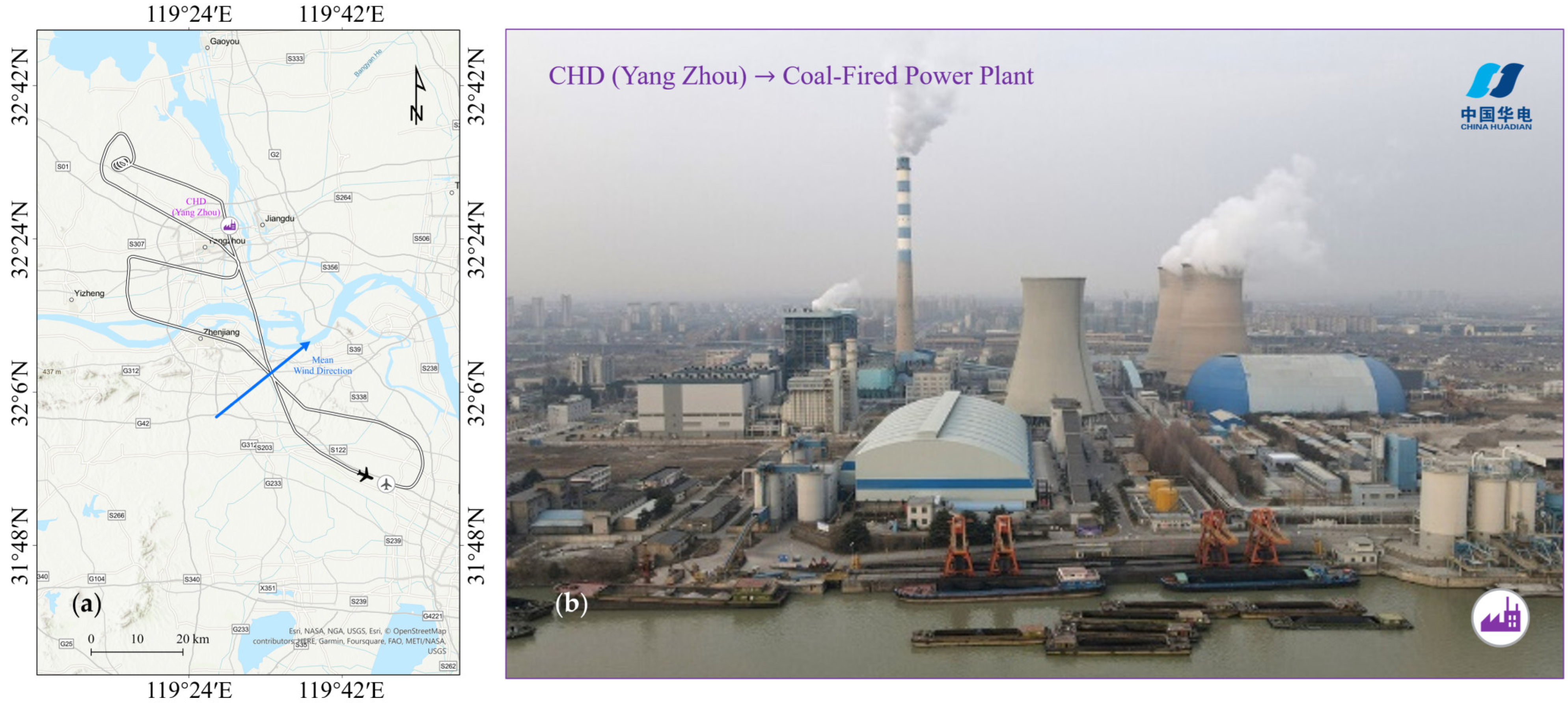
5.1. Aircraft Measurement of Power Plant Plumes
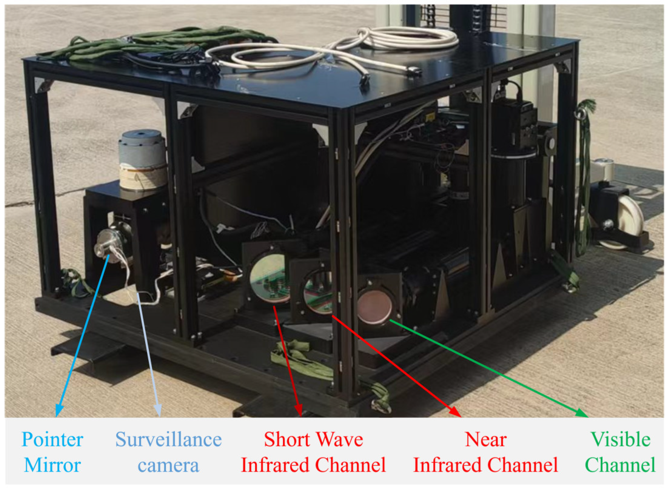
5.1.1. Instruments and Experimental Subject
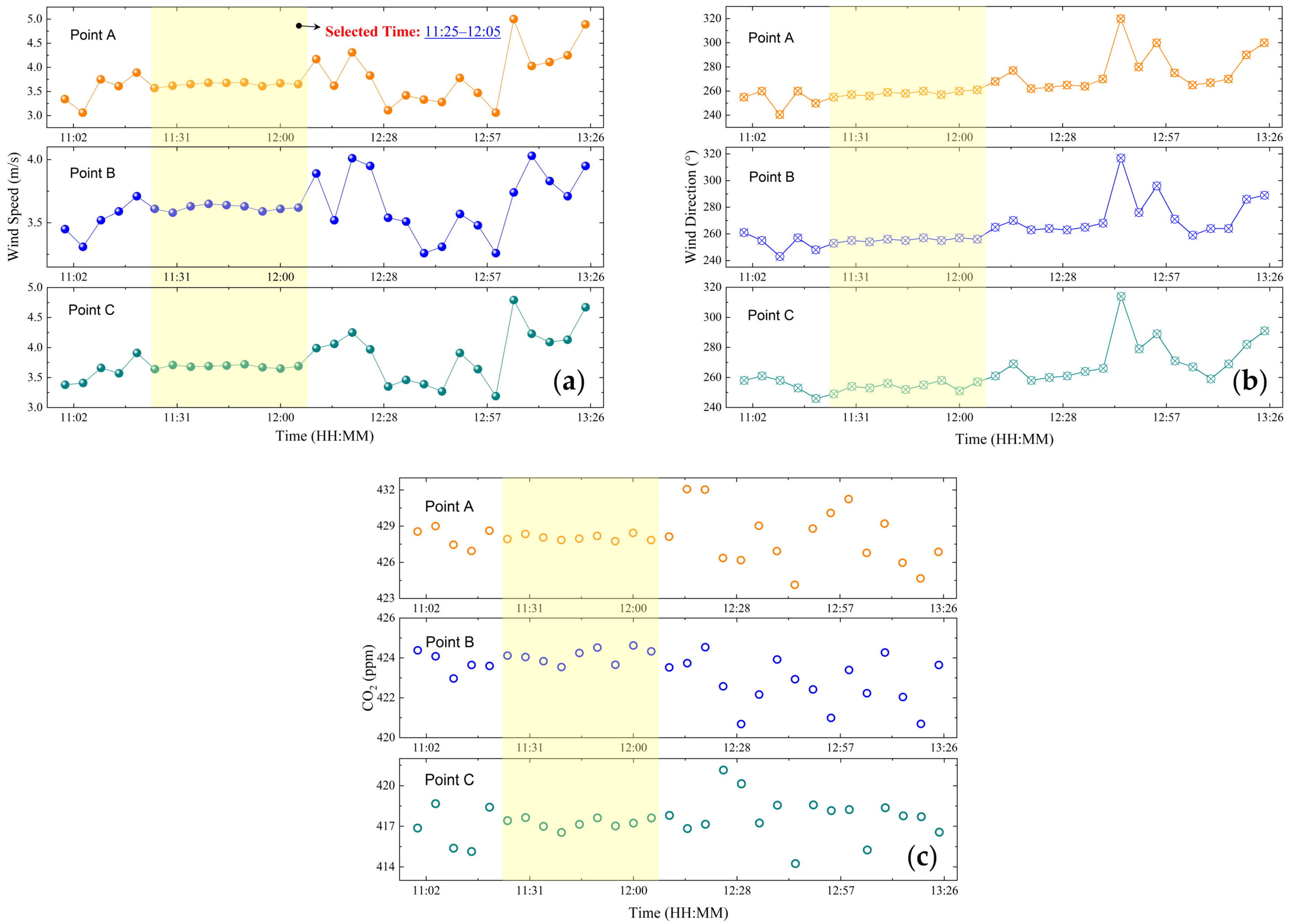
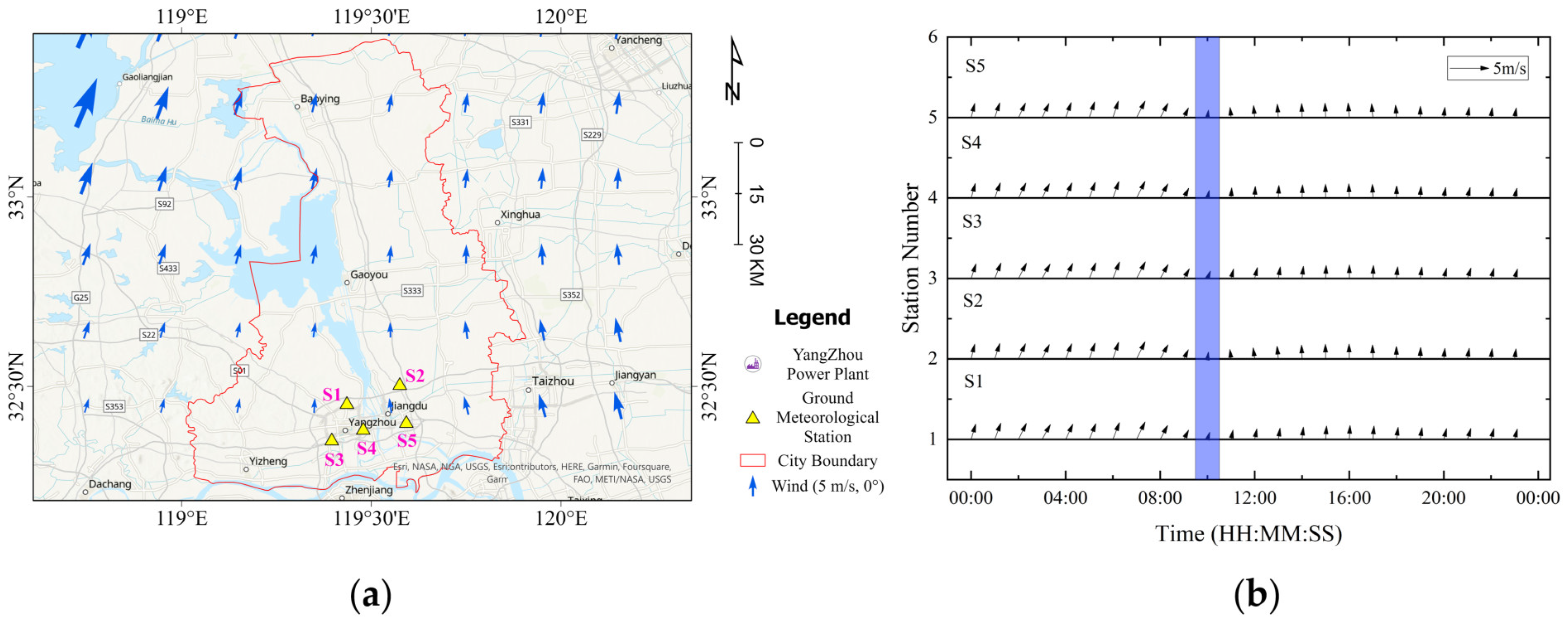
5.1.2. Ground Meteorological Observation
5.2. Model Parameters Setting
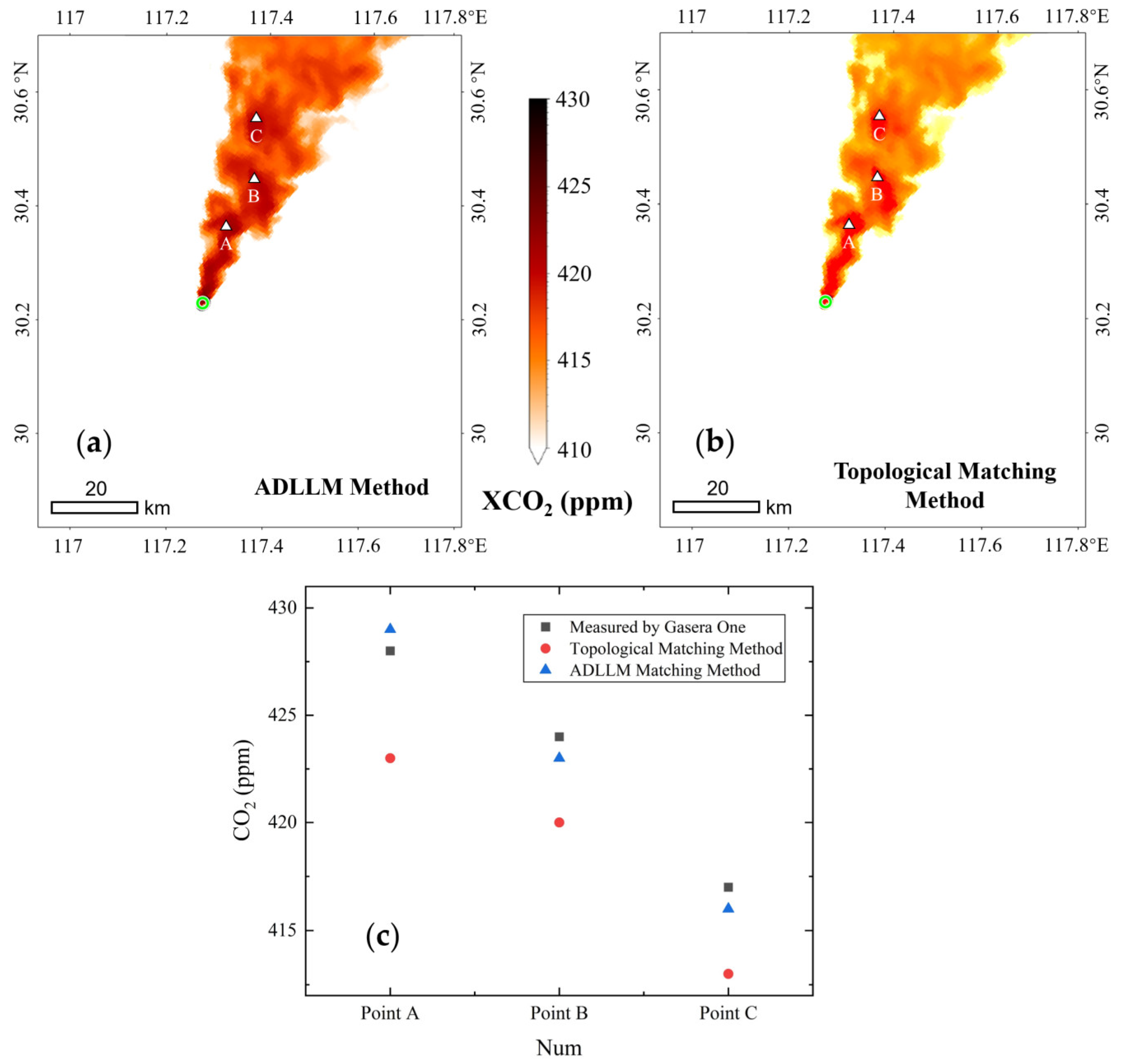
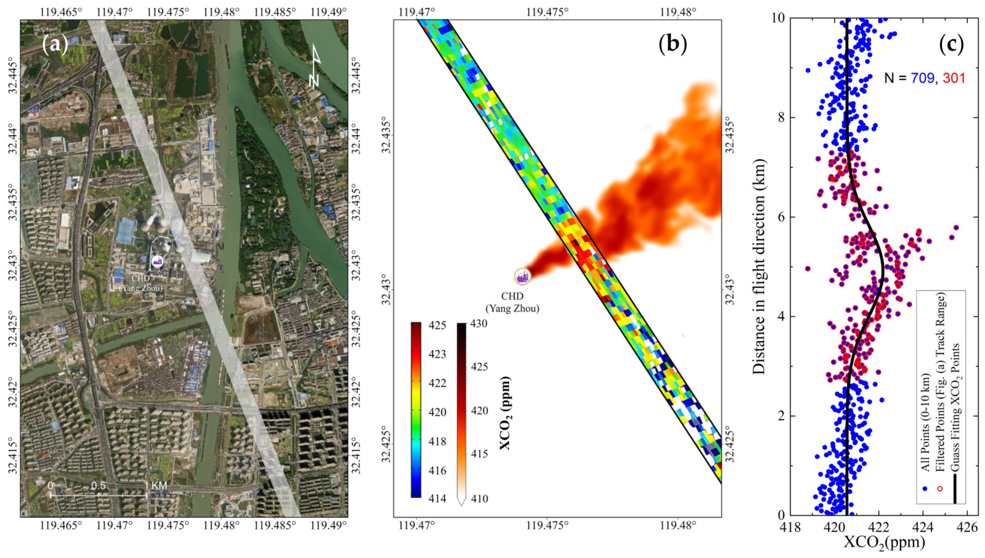
5.3. Quantitative Comparison and Analysis
6. Conclusions
Author Contributions
Funding
Data Availability Statement
Acknowledgments
Conflicts of Interest
References
- Pörtner, H.-O.; Roberts, D.C.; Adams, H.; Adler, C.; Aldunce, P.; Ali, E.; Begum, R.A.; Betts, R.; Kerr, R.B.; Biesbroek, R. Climate Change 2022: Impacts, Adaptation and Vulnerability; IPCC Sixth Assessment Report; IPCC: Geneva, Switzerland, 2022. [Google Scholar]
- Lamb, W.F.; Wiedmann, T.; Pongratz, J.; Andrew, R.; Crippa, M.; Olivier, J.G.J.; Wiedenhofer, D.; Mattioli, G.; Al Khourdajie, A.; House, J. A Review of Trends and Drivers of Greenhouse Gas Emissions by Sector from 1990 to 2018. Environ. Res. Lett. 2021, 16, 073005. [Google Scholar] [CrossRef]
- Whitaker, M.; Heath, G.A.; O’Donoughue, P.; Vorum, M. Life Cycle Greenhouse Gas Emissions of Coal-fired Electricity Generation: Systematic Review and Harmonization. J. Ind. Ecol. 2012, 16, S53–S72. [Google Scholar] [CrossRef]
- Butz, A.; Guerlet, S.; Hasekamp, O.; Schepers, D.; Galli, A.; Aben, I.; Frankenberg, C.; Hartmann, J.; Tran, H.; Kuze, A.; et al. Toward Accurate CO2 and CH4 Observations from GOSAT. Geophys. Res. Lett. 2011, 38, 14. [Google Scholar] [CrossRef]
- Wunch, D.; Wennberg, P.O.; Osterman, G.; Fisher, B.; Naylor, B.; Roehl, C.M.; O’Dell, C.; Mandrake, L.; Viatte, C.; Kiel, M. Comparisons of the Orbiting Carbon Observatory-2 (OCO-2) XCO2 Measurements with TCCON. Atmos. Meas. Tech. 2017, 10, 2209–2238. [Google Scholar] [CrossRef]
- Liu, Y.; Yang, D.; Cai, Z. A Retrieval Algorithm for TanSat XCO2 Observation: Retrieval Experiments Using GOSAT Data. Chin. Sci. Bull. 2013, 58, 1520–1523. [Google Scholar] [CrossRef]
- Ye, H.; Shi, H.; Li, C.; Wang, X.; Xiong, W.; An, Y.; Wang, Y.; Liu, L. A Coupled BRDF CO2 Retrieval Method for the GF-5 GMI and Improvements in the Correction of Atmospheric Scattering. Remote Sens. 2022, 14, 488. [Google Scholar] [CrossRef]
- Cao, X.; Zhang, L.; Zhang, X.; Yang, S.; Deng, Z.; Zhang, X.; Jiang, Y. Study on the Impact of the Doppler Shift for CO2 Lidar Remote Sensing. Remote Sens. 2022, 14, 4620. [Google Scholar] [CrossRef]
- Guerlet, S.; Butz, A.; Schepers, D.; Basu, S.; Hasekamp, O.P.; Kuze, A.; Yokota, T.; Blavier, J.; Deutscher, N.M.; Griffith, D.W.T. Impact of Aerosol and Thin Cirrus on Retrieving and Validating XCO2 from GOSAT Shortwave Infrared Measurements. J. Geophys. Res. Atmos. 2013, 118, 4887–4905. [Google Scholar] [CrossRef]
- Cai, Z.N.; Liu, Y.; Yang, D.X. Analysis of XCO2 Retrieval Sensitivity Using Simulated Chinese Carbon Satellite (TanSat) Measurements. Sci. China Earth Sci. 2014, 57, 1919–1928. [Google Scholar] [CrossRef]
- Nguyen, H.; Cressie, N.; Hobbs, J. Sensitivity of Optimal Estimation Satellite Retrievals to Misspecification of the Prior Mean and Covariance, with Application to OCO-2 Retrievals. Remote Sens. 2019, 11, 2770. [Google Scholar] [CrossRef]
- Laughner, J.L.; Roche, S.; Kiel, M.; Toon, G.C.; Wunch, D.; Baier, B.C.; Biraud, S.; Chen, H.; Kivi, R.; Laemmel, T.; et al. A New Algorithm to Generate A Priori Trace Gas Profiles for the GGG2020 Retrieval Algorithm. Atmos. Meas. Tech. 2023, 16, 1121–1146. [Google Scholar] [CrossRef]
- Kulawik, S.S.; Jones, D.B.A.; Nassar, R.; Irion, F.W.; Worden, J.R.; Bowman, K.W.; Machida, T.; Matsueda, H.; Sawa, Y.; Biraud, S.C.; et al. Characterization of Tropospheric Emission Spectrometer (TES) CO2 for Carbon Cycle Science. Atmos. Chem. Phys. 2010, 10, 5601–5623. [Google Scholar] [CrossRef]
- Landgraf, J.; Scheepmaker, R.; Borsdorff, T.; Hu, H.; Houweling, S.; Butz, A.; Aben, I.; Hasekamp, O. Carbon Monoxide Total Column Retrievals from TROPOMI Shortwave Infrared Measurements. Atmos. Meas. Tech. 2016, 9, 4955–4975. [Google Scholar] [CrossRef]
- Malina, E.; Hu, H.; Landgraf, J.; Veihelmann, B. A Study of Synthetic 13CH4 Retrievals from TROPOMI and Sentinel-5/UVNS. Atmos. Meas. Tech. 2019, 12, 6273–6301. [Google Scholar] [CrossRef]
- Holmes, N.S.; Morawska, L. A Review of Dispersion Modelling and its Application to the Dispersion of Particles: An Overview of Different Dispersion Models Available. Atmos. Environ. 2006, 40, 5902–5928. [Google Scholar] [CrossRef]
- Oettl, D.; Kukkonen, J.; Almbauer, R.A.; Sturm, P.J.; Pohjola, M.; Härkönen, J. Evaluation of a Gaussian and a Lagrangian Model against a Roadside Data Set, with Emphasis on Low Wind Speed Conditions. Atmos. Environ. 2001, 35, 2123–2132. [Google Scholar] [CrossRef]
- Stohl, A.; Forster, C.; Frank, A.; Seibert, P.; Wotawa, G. The Lagrangian Particle Dispersion Model FLEXPART Version 6.2. Atmos. Chem. Phys. 2005, 5, 2461–2474. [Google Scholar] [CrossRef]
- Jing, Y.; Wang, T.; Zhang, P.; Chen, L.; Xu, N.; Ma, Y. Global Atmospheric CO2 Concentrations Simulated by GEOS-Chem: Comparison with GOSAT, Carbon Tracker and Ground-Based Measurements. Atmosphere 2018, 9, 175. [Google Scholar] [CrossRef]
- Callewaert, S.; Brioude, J.; Langerock, B.; Duflot, V.; Fonteyn, D.; Müller, J.F.; Metzger, J.M.; Hermans, C.; Kumps, N.; Ramonet, M.; et al. Analysis of CO2, CH4, and CO Surface and Column Concentrations Observed at Réunion Island by Assessing WRF-Chem Simulations. Atmos. Chem. Phys. 2022, 22, 7763–7792. [Google Scholar] [CrossRef]
- Belikov, D.A.; Maksyutov, S.; Ganshin, A.; Zhuravlev, R.; Deutscher, N.M.; Wunch, D.; Feist, D.G.; Morino, I.; Parker, R.J.; Strong, K.; et al. Study of the footprints of short-term variation in XCO2 observed by TCCON sites using NIES and FLEXPART atmospheric transport models. Atmos. Chem. Phys. 2017, 17, 143–157. [Google Scholar] [CrossRef]
- Hu, C.; Zhang, M.; Xiao, W.; Wang, Y.; Wang, W.; Tim, G.; Liu, S.; Li, X. Tall tower CO2 concentration simulation using the WRF-STILT model. China Environ. Sci. 2017, 37, 2424–2437. [Google Scholar]
- Viatte, C.; Lauvaux, T.; Hedelius, J.K.; Parker, H.; Chen, J.; Jones, T.; Franklin, J.E.; Deng, A.J.; Gaudet, B.; Verhulst, K.; et al. Methane emissions from dairies in the Los Angeles Basin. Atmos. Chem. Phys. 2017, 17, 7509–7528. [Google Scholar] [CrossRef]
- Hedelius, J.K.; Liu, J.; Oda, T.; Maksyutov, S.; Roehl, C.M.; Iraci, L.T.; Podolske, J.R.; Hillyard, P.W.; Liang, J.; Gurney, K.R.; et al. Southern California megacity CO2, CH4, and CO flux estimates using ground-and space-based remote sensing and a Lagrangian model. Atmos. Chem. Phys. 2018, 18, 16271–16291. [Google Scholar] [CrossRef]
- Bezyk, Y.; Oshurok, D.; Dorodnikov, M.; Sówka, I. Evaluation of the CALPUFF model performance for the estimation of the urban ecosystem CO2 flux. Atmos. Pollut. Res. 2021, 12, 260–277. [Google Scholar] [CrossRef]
- Brunner, D.; Kuhlmann, G.; Henne, S.; Koene, E.; Kern, B.; Wolff, S.; Voigt, C.; Jöckel, P.; Kiemle, C.; Roiger, A.; et al. Evaluation of Simulated CO2 Power Plant Plumes from Six High-Resolution Atmospheric Transport Models. Atmos. Chem. Phys. 2023, 23, 2699–2728. [Google Scholar] [CrossRef]
- Cusworth, D.H.; Duren, R.M.; Thorpe, A.K.; Eastwood, M.L.; Green, R.O.; Dennison, P.E.; Frankenberg, C.; Heckler, J.W.; Asner, G.P.; Miller, C.E. Quantifying Global Power Plant Carbon Dioxide Emissions with Imaging Spectroscopy. AGU Adv. 2021, 2, e2020AV000350. [Google Scholar] [CrossRef]
- Guanter, L.; Irakulis-Loitxate, I.; Gorroño, J.; Sánchez-García, E.; Cusworth, D.H.; Varon, D.J.; Cogliati, S.; Colombo, R. Mapping Methane Point Emissions with the PRISMA Spaceborne Imaging Spectrometer. Remote Sens. Environ. 2021, 265, 112671. [Google Scholar] [CrossRef]
- Zheng, T.; Nassar, R.; Baxter, M. Estimating Power Plant CO2 Emission Using OCO-2 XCO2 and High Resolution WRF-Chem Simulations. Environ. Res. Lett. 2019, 14, 085001. [Google Scholar] [CrossRef]
- O’Brien, D.M.; Polonsky, I.N.; Utembe, S.R.; Rayner, P.J. Potential of a Geostationary GeoCARB Mission to Estimate Surface Emissions of CO2, CH4 and CO in a Polluted Urban Environment: Case Study Shanghai. Atmos. Meas. Tech. 2016, 9, 4633–4654. [Google Scholar] [CrossRef]
- Khanduri, A.C.; Stathopoulos, T.; Bédard, C. Wind-Induced Interference Effects on Buildings—A Review of the State-of-the-Art. Eng. Struct. 1998, 20, 617–630. [Google Scholar] [CrossRef]
- Carvalho, D.; Rocha, A.; Gómez-Gesteira, M.; Santos, C. A Sensitivity Study of the WRF Model in Wind Simulation for an Area of High Wind Energy. Environ. Model. Softw. 2012, 33, 23–34. [Google Scholar] [CrossRef]
- Ragland, K.W. Multiple Box Model for Dispersion of Air Pollutants from Area Sources. Atmos. Environ. 1973, 7, 1017–1032. [Google Scholar] [CrossRef]
- Loh, Z.; Leuning, R.; Zegelin, S.; Etheridge, D.; Bai, M.; Naylor, T.; Griffith, D. Testing Lagrangian atmospheric dispersion modelling to monitor CO2 and CH4 leakage from geosequestration. Atmos. Environ. 2009, 43, 2602–2611. [Google Scholar] [CrossRef]
- Fallah-Shorshani, M.; Shekarrizfard, M.; Hatzopoulou, M. Integrating a Street-Canyon Model with a Regional Gaussian Dispersion Model for Improved Characterisation of near-Road Air Pollution. Atmos. Environ. 2017, 153, 21–31. [Google Scholar] [CrossRef]
- Tuccella, P.; Curci, G.; Visconti, G.; Bessagnet, B.; Menut, L.; Park, R.J. Modeling of Gas and Aerosol with WRF/Chem over Europe: Evaluation and Sensitivity Study. J. Geophys. Res. Atmos. 2012, 117. [Google Scholar] [CrossRef]
- Lin, J.C.; Gerbig, C.; Wofsy, S.C.; Andrews, A.E.; Daube, B.C.; Davis, K.J.; Grainger, C.A. A Near-field Tool for Simulating the Upstream Influence of Atmospheric Observations: The Stochastic Time-Inverted Lagrangian Transport (STILT) Model. J. Geophys. Res. Atmos. 2003, 108, D16. [Google Scholar] [CrossRef]
- MacIntosh, D.L.; Stewart, J.H.; Myatt, T.A.; Sabato, J.E.; Flowers, G.C.; Brown, K.W.; Hlinka, D.J.; Sullivan, D.A. Use of CALPUFF for Exposure Assessment in a Near-Field, Complex Terrain Setting. Atmos. Environ. 2010, 44, 262–270. [Google Scholar] [CrossRef]
- Brecht, R.; Bakels, L.; Bihlo, A.; Stohl, A. Improving Trajectory Calculations by FLEXPART 10.4+ Using Single-Image Super-Resolution. Geosci. Model Dev. 2023, 16, 2181–2192. [Google Scholar] [CrossRef]
- Zhang, H.; Prater, M.D.; Rossby, T. Isopycnal Lagrangian Statistics from the North Atlantic Current RAFOS Float Observations. J. Geophys. Res. Oceans 2001, 106, 13817–13836. [Google Scholar] [CrossRef]
- Rizza, U.; Miglietta, M.M.; Mangia, C.; Ielpo, P.; Morichetti, M.; Iachini, C.; Virgili, S.; Passerini, G. Sensitivity of WRF-Chem Model to Land Surface Schemes: Assessment in a Severe Dust Outbreak Episode in the Central Mediterranean (Apulia Region). Atmos. Res. 2018, 201, 168–180. [Google Scholar] [CrossRef]
- Yerramilli, A.; Challa, V.S.; Dodla, V.B.R.; Dasari, H.P.; Young, J.H.; Patrick, C.; Baham, J.M.; Hughes, R.L.; Hardy, M.G.; Swanier, S.J. Simulation of Surface Ozone Pollution in the Central Gulf Coast Region Using WRF/Chem Model: Sensitivity to PBL and Land Surface Physics. Adv. Meteorol. 2010, 2010, 319138. [Google Scholar] [CrossRef]
- ul Haq, A.; Nadeem, Q.; Farooq, A.; Irfan, N.; Ahmad, M.; Ali, M.R. Assessment of Lagrangian Particle Dispersion Model “LAPMOD” through Short Range Field Tracer Test in Complex Terrain. J. Environ. Radioact. 2019, 205, 34–41. [Google Scholar] [CrossRef] [PubMed]
- Cécé, R.; Bernard, D.; Brioude, J.; Zahibo, N. Microscale Anthropogenic Pollution Modelling in a Small Tropical Island during Weak Trade Winds: Lagrangian Particle Dispersion Simulations Using Real Nested LES Meteorological Fields. Atmos. Environ. 2016, 139, 98–112. [Google Scholar] [CrossRef]
- Hill, T.; Nassar, R. Pixel Size and Revisit Rate Requirements for Monitoring Power Plant CO2 Emissions from Space. Remote Sens. 2019, 11, 1608. [Google Scholar] [CrossRef]
- Levy, P.E.; Cannell, M.G.R.; Friend, A.D. Modelling the Impact of Future Changes in Climate, CO2 Concentration and Land Use on Natural Ecosystems and the Terrestrial Carbon Sink. Glob. Environ. Chang. 2004, 14, 21–30. [Google Scholar] [CrossRef]
- Abrams, M.; Crippen, R.; Fujisada, H. ASTER Global Digital Elevation Model (GDEM) and ASTER Global Water Body Dataset (ASTWBD). Remote Sens. 2020, 12, 1156. [Google Scholar] [CrossRef]
- Nitheshnirmal, S.; Thilagaraj, P.; Rahaman, S.A.; Jegankumar, R. Erosion Risk Assessment through Morphometric Indices for Prioritisation of Arjuna Watershed Using ALOS-PALSAR DEM. Model. Earth Syst. Environ. 2019, 5, 907–924. [Google Scholar] [CrossRef]
- Wu, W.-B.; Ma, J.; Banzhaf, E.; Meadows, M.E.; Yu, Z.-W.; Guo, F.-X.; Sengupta, D.; Cai, X.-X.; Zhao, B. A First Chinese Building Height Estimate at 10 m Resolution (CNBH-10 m) Using Multi-Source Earth Observations and Machine Learning. Remote Sens. Environ. 2023, 291, 113578. [Google Scholar] [CrossRef]
- Park, J.-H.; Nam, W.-J.; Lee, S.-W. A Two-Stream Symmetric Network with Bidirectional Ensemble for Aerial Image Matching. Remote Sens. 2020, 12, 465. [Google Scholar] [CrossRef]
- Chen, Y.; Jiang, J. A Two-Stage Deep Learning Registration Method for Remote Sensing Images Based on Sub-Image Matching. Remote Sens. 2021, 13, 3443. [Google Scholar] [CrossRef]
- Pun, C.-M.; Yuan, X.-C.; Bi, X.-L. Image Forgery Detection Using Adaptive Oversegmentation and Feature Point Matching. IEEE Trans. Inf. Forensics Secur. 2015, 10, 1705–1716. [Google Scholar]
- Zhao, F.; Huang, Q.; Gao, W. Image Matching by Normalized Cross-Correlation. In Proceedings of the 2006 IEEE International Conference on Acoustics Speech and Signal Processing Proceedings, Toulouse, France, 14–19 May 2006; Volume 2, p. II. [Google Scholar]
- Heo, Y.S.; Lee, K.M.; Lee, S.U. Robust Stereo Matching Using Adaptive Normalized Cross-Correlation. IEEE Trans. Pattern Anal. Mach. Intell. 2010, 33, 807–822. [Google Scholar]
- Gao, S. Boundary Matching Based Spatial Interpolation for Consecutive Block Loss Concealment. In Proceedings of the 2012 IEEE International Symposium on Multimedia, Irvine, CA, USA, 10–12 December 2012; pp. 128–132. [Google Scholar]
- Nagata, F.; Tokuno, K.; Mitarai, K.; Otsuka, A.; Ikeda, T.; Ochi, H.; Watanabe, K.; Habib, M.K. Defect Detection Method Using Deep Convolutional Neural Network, Support Vector Machine and Template Matching Techniques. Artif. Life Robot. 2019, 24, 512–519. [Google Scholar] [CrossRef]
- Lindner, C.; Bromiley, P.A.; Ionita, M.C.; Cootes, T.F. Robust and Accurate Shape Model Matching Using Random Forest Regression-Voting. IEEE Trans. Pattern Anal. Mach. Intell. 2014, 37, 1862–1874. [Google Scholar] [CrossRef]
- Poulenard, A.; Skraba, P.; Ovsjanikov, M. Topological Function Optimization for Continuous Shape Matching. In Proceedings of the Computer Graphics Forum; Wiley Online Library: Hoboken, NJ, USA, 2018; Volume 37, pp. 13–25. [Google Scholar]
- Velaga, N.R.; Quddus, M.A.; Bristow, A.L. Developing an Enhanced Weight-Based Topological Map-Matching Algorithm for Intelligent Transport Systems. Transp. Res. Part C Emerg. Technol. 2009, 17, 672–683. [Google Scholar] [CrossRef]
- Li, X.; He, F.; Cai, X.; Zhang, D.; Chen, Y. A Method for Topological Entity Matching in the Integration of Heterogeneous CAD Systems. Integr. Comput. Aided Eng. 2013, 20, 15–30. [Google Scholar] [CrossRef]
- Bolkas, D.; Fotopoulos, G.; Braun, A.; Tziavos, I.N. Assessing Digital Elevation Model Uncertainty Using GPS Survey Data. J. Surveying Eng. 2016, 142, 04016001. [Google Scholar] [CrossRef]
- Wang, S.; Dong, X.; Liu, G.; Gao, M.; Xiao, G.; Zhao, W.; Lv, D. GNSS RTK/UWB/DBA Fusion Positioning Method and Its Performance Evaluation. Remote Sens. 2022, 14, 5928. [Google Scholar] [CrossRef]
- Li, J.; Cui, W.; Chen, P.; Dong, X.; Chu, Y.; Sheng, J.; Zhang, Y.; Wang, Z.; Dong, F. Unraveling the Mechanism of Binary Channel Reactions in Photocatalytic Formaldehyde Decomposition for Promoted Mineralization. Appl. Catal. B Environ. 2020, 260, 118130. [Google Scholar] [CrossRef]
- Muravieva, E.A.; Kulakova, E.S. Overview of the Instrumentation Base for Monitoring Greenhouse Gases. Nanotekhnologii v Stroitel’stve 2022, 14, 62–69. [Google Scholar]
- Sánchez-Navarro, V.; Shahrokh, V.; Martínez-Martínez, S.; Acosta, J.A.; Almagro, M.; Martínez-Mena, M.; Boix-Fayos, C.; Díaz-Pereira, E.; Zornoza, R. Perennial Alley Cropping Contributes to Decrease Soil CO2 and N2O Emissions and Increase Soil Carbon Sequestration in a Mediterranean Almond Orchard. Sci. Total Environ. 2022, 845, 157225. [Google Scholar] [CrossRef] [PubMed]
- Ding, Y.; Luo, H.; Shi, H.; Li, Z.; Han, Y.; Li, S.; Xiong, W. Correction of Invalid Data Based on Spatial Dimension Information of a Temporally and Spatially Modulated Spatial Heterodyne Interference Imaging Spectrometer. Appl. Optics 2021, 60, 6614–6622. [Google Scholar] [CrossRef] [PubMed]
- Ye, H.; Shi, H.; Wang, X.; Sun, E.; Li, C.; An, Y.; Wu, S.; Xiong, W.; Li, Z.; Landgraf, J. Improving Atmospheric CO2 Retrieval Based on the Collaborative Use of Greenhouse Gases Monitoring Instrument and Directional Polarimetric Camera Sensors on Chinese Hyperspectral Satellite GF5-02. Geo-spatial Inf. Sci. 2023, 1–13. [Google Scholar] [CrossRef]
- Chelani, A.B. Estimating PM2.5 Concentration from Satellite Derived Aerosol Optical Depth and Meteorological Variables Using a Combination Model. Atmos. Pollut. Res. 2019, 10, 847–857. [Google Scholar] [CrossRef]
- Trenchev, P.; Dimitrova, M.; Avetisyan, D. Huge CH4, NO2, and CO Emissions from Coal Mines in the Kuznetsk Basin (Russia) Detected by Sentinel-5P. Remote Sens. 2023, 15, 1590. [Google Scholar] [CrossRef]


| Location Matching Method | References |
|---|---|
| Feature Points Matching (M1) 1 | Pun et al. [52] |
| Correlation Matching (M2) 1 | Zhao et al. [53] and Heo et al. [54] |
| Spatial Interpolation (M3) 1 | Gao. [55] |
| SVM (M4) 1 | Nagata et al. [56] |
| Random Forest (M5) 1 | Lindner et al. [57] |
| Topological Matching (M6) 1 | Poulenard et al. [58], Velaga et al. [59], and Li et al. [60] |
| ADLLM (M7) 1 | This method used in this paper. |
| GPS Matching (M8) 1 | Bolkas et al. [61] |
| Location Matching Method | R2 | MAE 1 | RMSE 1 |
|---|---|---|---|
| Feature Points Matching | 0.412 | 0.715 | 0.85 |
| Correlation Matching | 0.46 | 0.75 | 0.817 |
| Spatial Interpolation | 0.637 | 0.519 | 0.636 |
| SVM | 0.79 | 0.394 | 0.462 |
| Random Forest | 0.815 | 0.35 | 0.41 |
| Topological Matching | 0.861 | 0.276 | 0.353 |
| ADLLM | 0.962 | 0.14 | 0.167 |
| STD_WS 1 | STD_WD 1 | STD_CO2 1 | |
|---|---|---|---|
| Point A | 0.0474 | 2.0245 | 0.4785 |
| Point B | 0.0227 | 1.2472 | 0.2136 |
| Point C | 0.0485 | 2.6663 | 0.3687 |
| Point A 1 | Point B 1 | Point C 1 | |
|---|---|---|---|
| ADLLM Method | 0.3187 | 0.4076 | 0.6463 |
| Topological Matching Method | 2.047 | 2.5352 | 2.7772 |
| Parameters | Visible | NIR | SWIR |
|---|---|---|---|
| Center Wavelength () | 0.7561 | 1.5647 | 2.0407 |
| Spectral Resolution (nm) | 0.029 | 0.076 | 0.157 |
| Spectral Dimension Half Field of View (°) | 1.02 | 0.85 | 0.668 |
| System Focal Length (mm) | 372.8 | 436.05 | 421.6 |
| Detector Size | 1024 × 1024@13 | 640 × 512@20 | 320 × 256@30 |
| Integration Time (ms) | 35 | 80 | 35 |
| Power Plant | ) | ) | Stack Height (m) | Stack Radius (m) | Velocity (m/s) | Temperature (K) | Emission Intensity (Mt/yr) |
|---|---|---|---|---|---|---|---|
| CO2 | |||||||
| Yangzhou CHD | 32.4312 | 119.4853 | 180 | 7 | 6.56 | 323 | 53.02 |
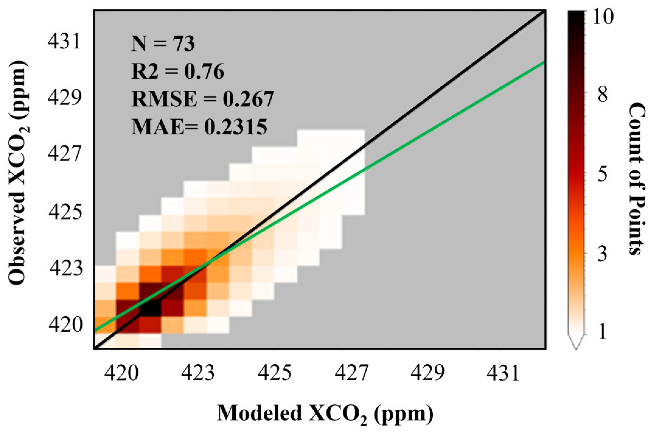
| Power Plant | Pixel Number 1 | Max Value 2 (ppm) | Min Value 2 (ppm) | Mean Value 2 (ppm) | R2 | MAE 3 | RMSE 3 |
|---|---|---|---|---|---|---|---|
| Yangzhou CHD | 73 | 428/425 | 412/410 | 418/416.3 | 0.76 | 0.2315 | 0.267 |
Disclaimer/Publisher’s Note: The statements, opinions and data contained in all publications are solely those of the individual author(s) and contributor(s) and not of MDPI and/or the editor(s). MDPI and/or the editor(s) disclaim responsibility for any injury to people or property resulting from any ideas, methods, instructions or products referred to in the content. |
© 2023 by the authors. Licensee MDPI, Basel, Switzerland. This article is an open access article distributed under the terms and conditions of the Creative Commons Attribution (CC BY) license (https://creativecommons.org/licenses/by/4.0/).
Share and Cite
Li, C.; Wang, X.; Ye, H.; Wu, S.; Shi, H.; Luo, H.; Li, Z.; Xiong, W.; Li, D.; Sun, E.; et al. Evaluation of Simulated CO2 Point Source Plumes from High-Resolution Atmospheric Transport Model. Remote Sens. 2023, 15, 4518. https://doi.org/10.3390/rs15184518
Li C, Wang X, Ye H, Wu S, Shi H, Luo H, Li Z, Xiong W, Li D, Sun E, et al. Evaluation of Simulated CO2 Point Source Plumes from High-Resolution Atmospheric Transport Model. Remote Sensing. 2023; 15(18):4518. https://doi.org/10.3390/rs15184518
Chicago/Turabian StyleLi, Chao, Xianhua Wang, Hanhan Ye, Shichao Wu, Hailiang Shi, Haiyan Luo, Zhiwei Li, Wei Xiong, Dacheng Li, Erchang Sun, and et al. 2023. "Evaluation of Simulated CO2 Point Source Plumes from High-Resolution Atmospheric Transport Model" Remote Sensing 15, no. 18: 4518. https://doi.org/10.3390/rs15184518