
Regional Gravity Field Modeling Using Band-Limited SRBFs: A Case Study in Colorado


1
School of Engineering Management and Real Estate, Henan University of Economics and Law, Zhengzhou 450002, China
2
School of Geospatial Engineering and Science, Sun Yat-sen University, Zhuhai 519082, China
3
Key Laboratory of Comprehensive Observation of Polar Environment, Sun Yat-sen University, Ministry of Education, Zhuhai 519082, China
4
School of Surveying and Land Information Engineering, Henan Polytechnic University, Jiaozuo 454000, China
*
Author to whom correspondence should be addressed.
Remote Sens. 2023, 15(18), 4515; https://doi.org/10.3390/rs15184515
Submission received: 27 August 2023
/
Revised: 12 September 2023
/
Accepted: 13 September 2023
/
Published: 14 September 2023
(This article belongs to the Section Engineering Remote Sensing)
Abstract
:The use of spherical radial basis functions (SRBFs) in regional gravity field modeling has become popular in recent years. However, to our knowledge, their potential for combining gravity data from multiple sources, particularly for data with different spectrum information in the frequency domain, has not been extensively explored. Therefore, band-limited SRBFs, which have good localization characteristics in the frequency domain, were taken as the main tool in this study. To determine the optimal expansion degree of SRBFs for gravity data, a residual and a priori accuracy comparative analysis method was proposed. Using this methodology, the expansion degrees of terrestrial and airborne data were determined to be 5200 and 1840, respectively, and then a high-resolution geoid model called ColSRBF2023 was constructed for use in Colorado. The results indicated that ColSRBF2023 had a standard deviation (STD) of 2.3 cm with respect to the GSVS17 validation data. This value was 2–6 mm lower than models obtained using different expansion degrees for gravity data and models from other institutions considered in this study. Furthermore, when comparing it with the validation geoid model on a 1′ × 1′ grid, ColSRBF2023 exhibited an STD value of 2.4 cm, which was also the best among the examined models. These findings highlight the importance of determining the optimal expansion degree of gravity data, particularly for constructing high-resolution gravity field models in rugged mountainous areas.
1. Introduction
Gravity data are crucial for studying the Earth’s gravity field and establishing the International Height Reference System (IHRS). Currently, global gravity field models (GGMs) are routinely used to provide long wavelength information for regional gravity field modeling. Apart from GGMs, terrestrial gravity data are the most widely used data type. However, in areas that are challenging to access (e.g., polar regions, mountains, forests, coastal areas, oceans) or in very large areas (e.g., >10,000 km2), airborne gravity practically becomes the only option [1]. In 2017, the Joint Working Group (JWG) 2.1.2 of the International Association of Geodesy (IAG) launched the Colorado geoid experiment (the 1 cm geoid experiment). The goal of this experiment is to assess the repeatability of gravity potential values as IHRS coordinates using different geoid modeling methods. In this context, the National Geodetic Survey (NGS) agreed to provide terrestrial gravity data, airborne gravity data, GPS/leveling data, and a digital terrain model for an area of approximately 500 km × 800 km in Colorado, which allowed the comparison of different methods for geoid computation using the same input dataset.
However, when using terrestrial and airborne gravity for local geoid refinement, there are several challenges that need to be addressed. First, terrestrial and airborne gravity data differ not only in spatial distribution and spectral content but also in their error characteristics. Therefore, a major challenge for geoid modeling is the proper combination of terrestrial and airborne gravity data. Second, both terrestrial and airborne gravity observations are unevenly distributed, leading to uncertainty in their spectral information. The spectral information of gravity data is closely related to their spatial resolution. However, determining the appropriate resolution of both terrestrial and airborne gravity data is difficult. The terrestrial gravity data resolution relies heavily on topographic heights, the distribution of which are usually extremely uneven, while the resolution of airborne gravity observations is influenced by factors such as the flight altitude, speed, and data correlation. All of these factors pose significant challenges in determining the optimal spectrum of gravity data. Third, for airborne gravity data, a downward continuation process is typically required [2,3,4]. However, the downward continuation process is an unstable procedure that amplifies high-frequency noise, leading to a reduction in the quality of airborne data. Moreover, a series of filtering and estimation techniques are usually required for airborne gravity data, which further exacerbate the uncertainty of the spectral information for airborne gravity data. It has been observed that using gravity signals beyond their corresponding spherical harmonic (SH) degree can introduce modeling errors [5]. Therefore, finding and modeling the useful information provided by gravity data has become a critical issue in local geoid enhancement [6].
Several methods can be employed to refine the regional geoid model, such as the well-known least squared collocation (LSC) method [7], least squares spectral combination method [8,9], and Slepian functions [10]. In this study, we chose to use band-limited spherical radial basis functions (SRBFs) for local geoid refinement. The justifications for this choice are as follows. First, the band-limited SRBFs can be adjusted flexibly based on the spectral information of the gravity data, which allows for better adaptation to the spectral characteristics of the gravity data. Second, band-limited SRBFs can express almost all types of gravity data, which form the basis for combining multisource gravity data to build a high-resolution regional gravity field model. Third, the band-limited SRBF expression includes a continuation factor, allowing the establishment of observation equations directly at scattered points of observation without the need for gridding or downward continuation. This feature enables the assignment of observation errors to specific observables in space. Li utilized a set of band-limited SRBFs to model gravity data and demonstrated that the SRBF method could effectively recover the gravity field while exhibiting filtering properties due to its design in the frequency domain. Additionally, experiments have shown that SRBFs are computationally efficient and do not require a covariance model such as the LSC method, which is sometimes time-consuming [11]. Other examples and explanations of SRBFs can also be found in [12,13,14,15,16,17,18,19,20,21] and the references therein.
In this study, our main focus is on refining the regional geoid model in Colorado using band-limited SRBFs. To determine the optimal spectral information of the gravity data, we propose a residual and a priori accuracy comparative analysis method. The organization of this work is as follows. In Section 2, we present the fundamental concepts of SRBFs and the parameter estimation procedure. This includes the formulation of observation equations, estimation of unknown coefficients, and calculation of gravitational functionals. In Section 3, we introduce the study area in Colorado and describe the available data. We also outline the procedure for data preprocessing. In Section 4, we explain the computation procedure, which involves the RCR procedure, the residual and a priori accuracy comparative analysis method, and how we combine different datasets. Section 5 presents our models as well as the validation of the results. Finally, Section 6 provides the conclusions and presents potential future research directions.
2. Theory and Methods
A residual harmonic function outside a sphere of radius R can be written as a finite sum of band-limited SRBFs:
where is the position vector of the observation point P, is the spherical longitude, is the spherical latitude, and , with being the spherical height of P above sphere with radius R. are the position vectors of the SRBFs. is the number of SRBFs, is the residual disturbing potential, and is the unknown coefficient. is a band-limited SRBF, the specific expression for which is [22]
where is the kernel function that defines the spectral properties of the SRBFs, is the mean radius of Earth, is the Legendre polynomial of degree , and is the spherical distance between and . and are the minimum and maximum degrees of expansion, respectively. The SRBF in Equation (2) is band-limited since the kernel functions are zero for each degree beyond or below .
The general expression of Equation (2) needs to be adapted to describe different gravitational functionals. We use observations that are given in terms of gravity disturbances , which can be expressed as the gradient of the disturbing potential . In the spherical approximation, the magnitude of the gravity disturbance can be written as [23]
From the SRBF expression for the disturbing potential (Equation (1)), the residual terrestrial gravity disturbances at the Earth’s surface and the residual airborne gravity disturbances at flight altitude can be written as
where and represent the position vectors of terrestrial and airborne gravity disturbances, respectively. and are the maximum degrees of expansion of the terrestrial and airborne gravity disturbances, respectively. are the adapted SRBFs of .
For terrestrial gravity observations, it is difficult to obtain a more appropriate expansion degree due to their uneven distribution. For airborne gravity data, however, due to their high altitudes and the low-pass filtering process, it is also not a simple task to determine optimal spectral information. In this study, we provide a way to determine the optimal degree of series expansion for gravity data ( and ), which will be introduced in Section 4.2.
In Equation (4), terrestrial gravity disturbances and airborne gravity disturbances have the same SRBF coefficients , and we can thus combine them to form the observation equations (Gauss–Markov model)
where and are the vectors of the terrestrial and airborne gravity disturbances, and and are the design matrices. are the unknown SRBF coefficients, and and are the vectors of observation errors with expectation and dispersion . is the variance-covariance matrix of the observed error and meets ; and are the observation weight matrices for group .
Usually, the normal equation matrix of Equation (5) is ill conditioned, and stabilization is needed to make the computation of a solution possible. Moreover, since the true accuracy of the two datasets is not exactly known, it is especially necessary to determine reasonable variance factors when building the gravity field model by combining terrestrial and airborne gravity data. All of these requirements can be met using the variance component estimation method (VCE) [24]
where and are the variance factors of terrestrial and airborne gravity disturbances, respectively. is the variance factor of unknown coefficients, which is also a regularization parameter, and is the unit matrix. The variance factors are usually determined based on an iterative method. Specifically, the initial variance factors ,, and are first given, and then the initial SRBF coefficients are estimated with the least squares estimation method. Then, the residuals of the least square values of the observations are further obtained, and the new variance factors can be calculated by
where and are the residuals after the th iteration, are the variance factors of the th group of observations after the th iteration, and is the variance factor of the unknown coefficients. and are redundant numbers, which can be expressed as
where represents the number of gravity observations of group , is the number of coefficients of SRBFs, is the design matrix at the th iteration, is the matrix of the normal equation at the th iteration, and is the total normal equation matrix at the th iteration. stands for trace operation. For the computation of the partial redundancies in Equations (9) and (10), the inverse matrix of normal equations is needed. We use the stochastic trace estimation theorem proposed by Hutchinson [25].
After the new variance factors are calculated, the next loop is entered until the convergence condition of the following equation is satisfied:
where is the convergence threshold, and we set in this study.
Applying the least squares method to Equation (6), the unknown coefficients are estimated as
Inserting the coefficients of Equation (12) back into Equation (1), we can obtain the residual disturbing potential .
The residual height anomaly is related to the residual disturbing potential by
where is the normal gravity defined at the telluroid and is the residual height anomaly.
Then, during the recovery procedure, we add back the height anomaly component of the GGM and the topographic effects, and a full-wavelength height anomaly can be obtained.
Finally, the geoid undulation can be obtained by the following conversion:
where is the orthometric height, is the geoid undulation, and is the simple Bouguer anomaly. Higher-order terms of the separation term [26] are not considered here, to be consistent with previously published procedures.
3. Gravity Data Processing and Analysis
3.1. Area of Interest
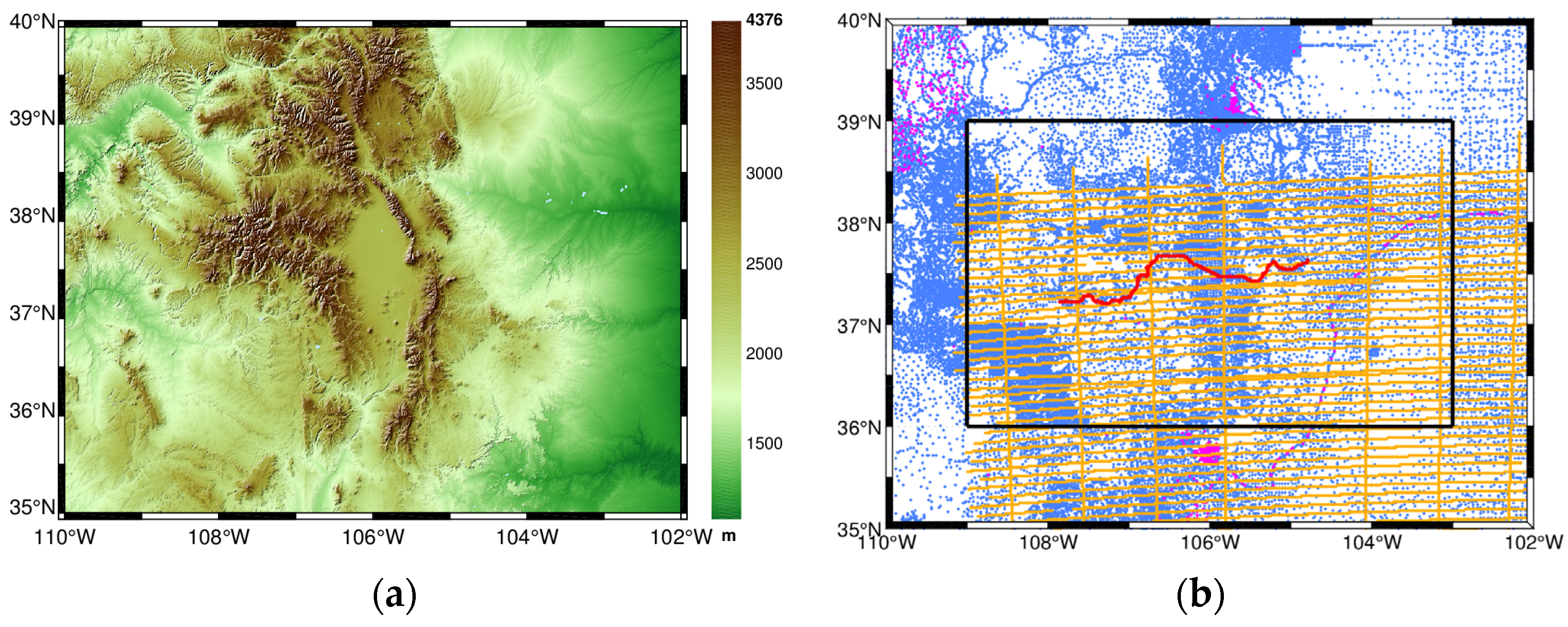
The Colorado geoid computation experiment is a collaborative effort involving the international geodetic community [27]. The study region is located between −110° and −102° longitude and between 35° and 40° latitude, primarily within the state of Colorado, USA. The area is characterized by mostly rugged terrain, which is evident in the topographic map displayed in Figure 1a. The average elevation in this region is approximately 2017 m. The highest peak reaches an elevation of 4376 m, while the lowest point is at 932 m. The St. Louis Valley, which is an extensive depositional basin, is situated in the central part of the study area. It covers an approximate area of 21,000 km2. To the west of the St. Louis Valley are the San Juan Mountains, which comprise a rugged mountain range of the Rocky Mountains. The eastern part of the study area consists of a plateau where the terrain is relatively flatter compared to other regions. This geographical information is important in understanding the challenges of the study area in refining the regional geoid model in Colorado.
3.2. Datasets Used for Modeling
The available data for the Colorado geoid computation experiment include terrestrial and airborne gravity data, GSVS17 GPS/leveling data, and GGMs. The terrestrial gravity data were provided by the National Geodetic Survey (NGS) and consist of 59,303 values obtained from over 137 survey campaigns, covering the entire area of the Colorado geoid project (see Figure 1b). Grigoriadis et al. studied the spatial density of the point values for the area, and the results found that only 21.25% of the total cells of the grid contain at least 1 point value, and approximately 50% of the cells of the grid contain at least one value [28]. Therefore, it is more reasonable to build a geoid model with a resolution of less than .
The raw airborne data use the Gravity for the Redefinition of the American Vertical Datum (GRAV-D) Block MS05. The east-west track spacing is 10 km, while the north-south cross-track spacing is 80 km. The mean flight altitude is approximately 6200 m. Figure 1b illustrates the distributions of the survey lines in the area. As shown in Figure 1b, the lines are relatively evenly distributed and cover most of the study area. However, the coverage of airborne and terrestrial gravity data does not overlap completely. The airborne gravity data cover the latitudes between and longitudes between . There are no airborne data available for latitudes between and longitudes between (Figure 1b). Moreover, the raw gravity data from MS05 are subject to biases between different tracks. Therefore, data from MS05 were debiased using the maximum median technique [29] and then resampled to 1 Hz. Finally, a dataset consisting of 283,716 data points was obtained. In addition, the GRAV-D Team defines the Fourier wavelength of the smallest recoverable feature as [30]
where is the height of the measurement point above the center of the spherical body that causes the anomaly. In this study, the average altitude of the aircraft is 6.2 km, and the average topographic height is approximately 2 km; then, the distance of is approximately 4.2 km. By substituting into Equation (15), the minimum resolvable wavelength is calculated to be 12.9 km, corresponding to a spherical harmonic degree of approximately 1530. However, this is only a rough estimate of the resolution since the study area is mountainous and the topographic heights vary significantly.
Additionally, a total of 222 benchmarks of Geoid Slope Validation Survey 2017 (GSVS17) profile data [31] were provided by NGS. These benchmarks are spaced approximately 1.6 km along Highway US 160 from Durango to Walsenburg. The accuracy of the geoid undulations inferred from the GPS-based ellipsoidal heights and the leveling-based orthometric heights is estimated to be approximately 1.5 cm. In addition to the GSVS17 GPS/leveling data, a mean geoid model on a grid based on all models submitted to ISG is used as a validation model to assess the performance of geoid models over the entire area. Furthermore, the reference frame used for the 3-D positioning of all three types of data (terrestrial gravity, airborne gravity, and GSVS17) is the IGS Reference Frame 2008 (IGS08) [32] on the Geodetic Reference System 1980 (GRS80) ellipsoid [33].
3.3. Data Preprocessing
In the original terrestrial data, there are cases in which several gravity observations are located at the same position, for which we only use the first of these observations (1090 points deleted). However, if the points share the same location but have a height difference of more than 3 m or a gravity difference of more than 2 mGal, then these points are both removed. Hence, 1215 points in total are excluded from the dataset (see Figure 1b). Finally, a total of 58,088 terrestrial gravity observations in the modeling area are obtained. Moreover, since the measurements are provided in orthometric heights H, we transform them to ellipsoidal heights using the geoid model GEOID18B [34]. This geoid model is a hybrid model specifically designed to convert GPS observations given in NAD83 ellipsoid heights to orthometric heights that are consistent with NAVD88. The airborne data have a dense distribution, resulting in a large design matrix. To simplify the computations, the sampling interval is reduced from 1 Hz to 1/8 Hz, and an average spatial interval of approximately 1 km along-track is obtained. This results in a total of 31,069 airborne gravity observations in the modeling area.
Then, for both types of observations, the following data preprocessing steps are performed.
① The observations are converted from absolute gravity to gravity disturbances by subtracting the normal gravity at the ellipsoidal height of the observations.
② The atmospheric corrections are calculated using the method proposed by Torge [35].
③ Atmospheric corrections are added to the gravity disturbances .
3.4. Remove Procedure
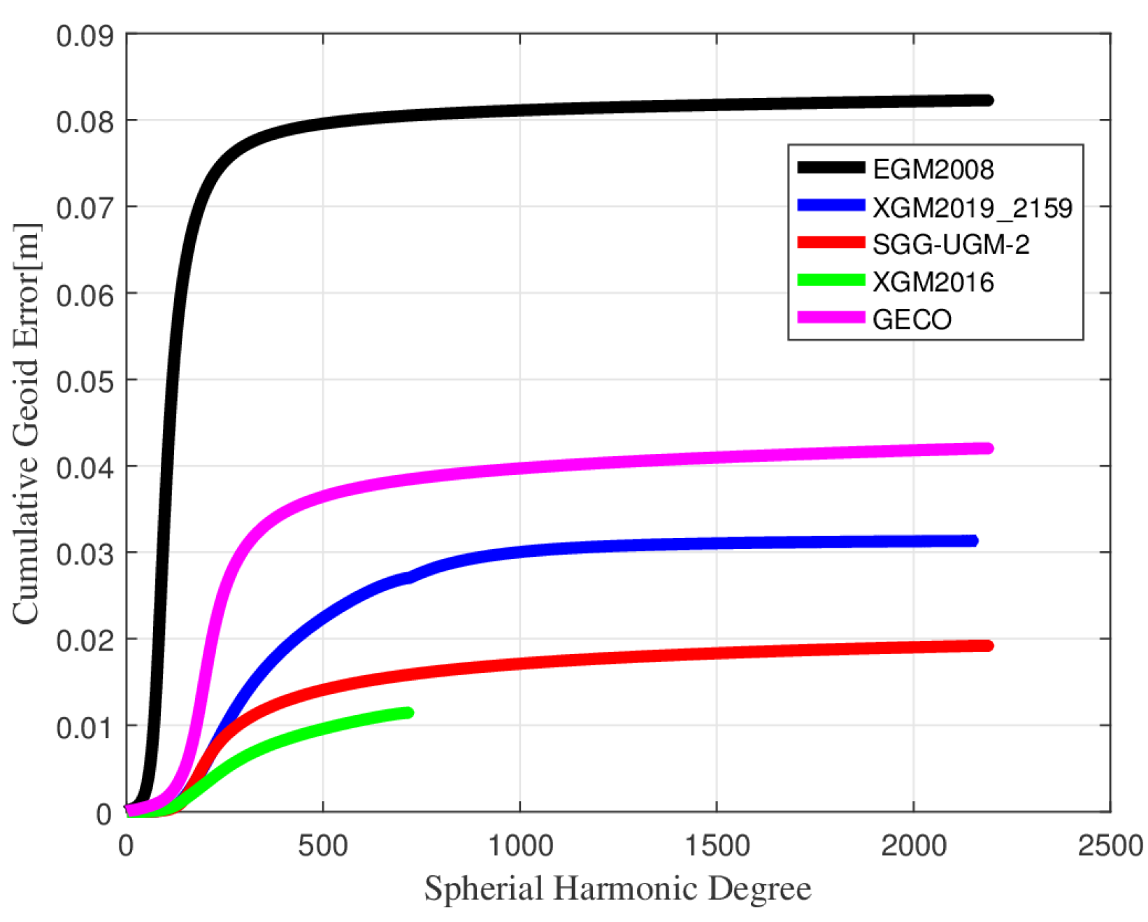
Gravity data obtained in a limited area cannot resolve long wavelengths in the gravity field. Therefore, the remove–compute–restore (RCR) procedure is usually utilized to remove the low-frequency and high-frequency signals of gravity data before modeling. However, when applying the RCR procedure, it is important to assess the performance of the GGMs, as the error of the GGMs accumulates as the expansion degrees increase. In this study, five combined GGMs are investigated: EGM2008 [36], XGM2019e_2159 [37], SGG-UGM-2 [38], XGM2016 [39], and GECO [40]. These models were chosen because they have relatively high accuracies and better spatial resolutions compared to other GGMs. The error degree variance offers insight into the error of a GGM, and it supplies a rudimentary quality assessment [41]. Figure 2 shows the degreewise accumulated geoid errors of the five GGMs. EGM2008 exhibits a relatively large error, which rapidly increases from degrees 30 to 220, reaching approximately 7.3 cm at degree 220, and then slowly increases to 8.2 cm at the highest degree. On the other hand, models such as XGM2019e_2159, SGG-UGM-2, and GECO, which have similar expansion degrees, show reduced errors of approximately 3.1 cm, 1.9 cm, and 4.3 cm, respectively. The significant error in EGM2008 in the frequency bands between degrees 30 and 220 is mainly due to the lack of data from the gravity field and steady-state GOCE satellite. In contrast, the other three models are developed using GOCE data, resulting in better quality in these frequency bands. Among the investigated models, XGM2016 exhibits the minimum cumulative geoid height error. Up to degree 719, the cumulative geoid height error of XGM2016 is approximately 1.1 cm, which is significantly lower than the corresponding values of the other four GGMs. Therefore, the XGM2016 model up to degree 719 is chosen for the RCR procedure. It is important to note that the error degree variance only provides a global mean of the internal error and cannot be considered as a realistic error estimate [42].
Another important factor that influences the performance of geoid modeling is topographic effects, which play a key role in mountainous areas since they can smooth the input observations and are of the utmost importance in obtaining a good least squares fit. The topographic model dV_ELL_Earth2014 [43] from degree 720 to degree 2159 and a residual terrain model ERTM2160 [44] from degree 2160 to degree ~80,000 are removed from the terrestrial data. Similarly, for the airborne data, the effect of dV_ELL_Earth2104 from degree 720 to degree is removed. Notably, we use two different topographic models above degree 720 for the terrestrial and airborne data, which is reasonable because both the dV_ELL_Earth2014 and ERTM2160 models are derived from the same original data and contain the same signal. This approach ensures consistency and avoids introducing additional errors due to the use of different models. Notably, for airborne data, the effect of dV_ELL_Earth2104 from degree 720 to degree is removed. In contrast, previous studies have utilized different degrees for the removal of topographic contributions in airborne data. However, we believe that removing topographic effects with degrees exceeding the optimal expansion degree of the gravity data may introduce modeling errors. Therefore, in this study, we only remove the topographic contributions up to the expansion degree of the airborne data.
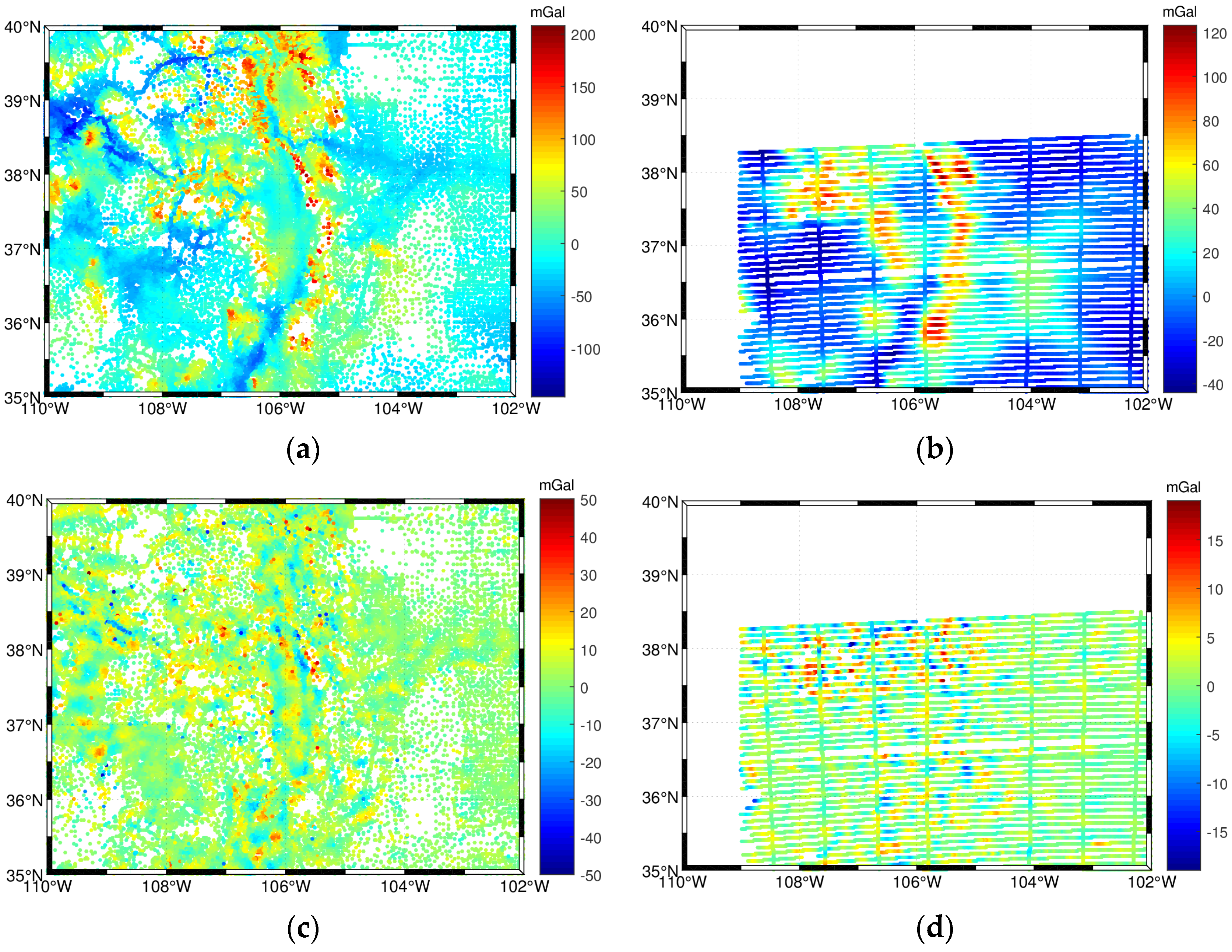
Figure 3 illustrates the distributions of the terrestrial and airborne gravity disturbances before and after the removal of the GGM and topographic effects. Figure 3a shows that the terrestrial gravity data have full coverage over the whole study area, but they are not evenly distributed. The dataset exhibits higher density in the central parts of the region and lower density in the eastern, northwestern, and southwestern parts. In contrast, the airborne data have relatively uniform coverage, although they do not cover the entire study area (Figure 3b). Figure 3c,d clearly show that the gravity disturbances become significantly smoother after subtracting the contributions of the GGM and topographic effects.
Table 1 presents the statistical results of the gravity observations. The standard deviations of the terrestrial and airborne gravity disturbances are reduced from 38.72 to 6.90 mGal and from 29.56 to 3.35 mGal, respectively. The standard deviation of the terrestrial data is reduced by 42.15% after subtracting the GGM and further reduced by 82.18% after including the topographic effects. Similarly, the airborne observations are reduced by 72.40% after subtracting the GGM and further reduced by 88.67% after including the topographic effects. The significant reduction in STD indicates that the removal of the GGM and topographic effects leads to a smoother gravity field, enabling a better least squares fit in the gravity field modeling using SRBFs. Notably, the smoothing effects are more pronounced in the terrestrial observations compared to the airborne observations after including the topographic model (Table 1). This is because the short-wavelength signal of the gravity field decreases with height, and the airborne gravity data are less sensitive to the short-wavelength part compared to the terrestrial gravity data. Consequently, subtracting the topographic effects has a greater influence on the terrestrial gravity data compared to the airborne gravity data. Illustrating the smoothing effects and quantifying the reduction in STD demonstrates the importance of removing the GGM and topographic contributions in obtaining a good least squares fit for gravity field modeling.
4. Gravity Field Modeling
In gravity field modeling based on band-limited SRBFs, several parameters and procedures are considered.
① Geocentric gravitational constant (): 3.986 004 415 × .
② Average density of topographic masses (): 2670 .
③ Geoid computations are performed in the tidefree system. GRS80 is used as the reference ellipsoid, and the conventional constants are taken from Moritz (2000).
Apart from these fundamental parameters, four important factors that influence the performance of SRBFs are also accounted for, namely (1) the type of the SRBFs; (2) the location of the SRBFs; (3) the extensions of the observation area, computation area, and target area; and (4) the maximum and minimum expansion degree of the SRBFs. Considering these parameters and procedures helps to ensure an effective and accurate gravity field modeling process based on band-limited SRBFs. Next, we introduce the model configuration for gravity field modeling based on band-limited SRBFs.
4.1. Model Configuration
4.1.1. Types of SRBFs
There are many types of SRBFs that can be used for gravity field modeling, such as the Shannon functions, the Blackman functions, the Poisson functions, and the cubic polynomial functions. The Shannon function is a reproducing kernel of the space spanned by all solid spherical harmonics of degrees [45]. As a result, it does not smooth the gravity signal in this spectral band. However, other types of SRBFs (e.g., Blackman functions, Poisson functions, and cubic polynomial functions) with nonconstant kernel functions might smooth some gravity field harmonics. Although some harmonic properties still remain in the recovered signal, they might be significantly suppressed. Therefore, one has to be careful when interpreting results based on the SRBFs with smoothing kernel functions. Moreover, Bentel et al. studied the performance of different types of SRBFs, and the results show that the Shannon SRBFs lead to the same results as with spherical harmonics both in theory and in practice. Therefore, in this study, the Shannon kernel functions are used, the specific form of which is
4.1.2. The Location of the SRBFs
The location of the SRBFs depends on the type of grid. There are many types of grids that can be used for regional gravity field modeling, such as the Driscoll–Healy grid, the triangle vertex grid, and the Reuter grid [46]. Eicker analyzed the advantages and disadvantages of different types of grids, and the results show that both the Reuter grids and the triangle vertex grids are suitable for gravity field modeling with SRBFs. Bentel et al. noted that different types of grids do not differ significantly, especially compared to the other three factors that influence the modeling results. In addition, the control parameter of the Reuter grids is related to the maximum expansion degree of SRBFs, which also facilitates gravity field modeling. We set , where is the maximum degree of the series expansion of SRBFs.
4.1.3. The Extensions of the Target, Observation, and Computation Area
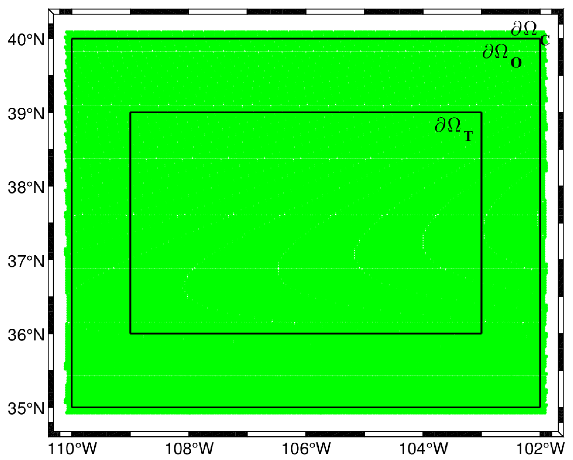
In regional gravity modeling, the extension of the target area , the observation area , and the computation area needs to be defined carefully. At the edge of the observation area , the unknown coefficients cannot be appropriately estimated, which provokes edge effects. In general, the target area should be smaller than the observation area , and the computation area should be larger than the observation area [47]. Therefore, to minimize the edge effects in the computation, should be satisfied. In addition, the margin size needs to be defined between the three areas. In our case, the target area is given to be between −109 and −103 and 36 and 39. Therefore, the margin size between and is fixed to 1.
The determination of the margin size between and follows the empirical formula described by Liu et al.:
where is the maximum latitude value of the study area. In this study, (see Section 4.3). By substituting this value into formula (20), the value follows. Figure 4 visualizes the target area, the observation area, the computation area, and the margins.
4.1.4. Maximum and Minimum Expansion Degree of SRBFs
The maximum degree of expansion of SRBFs is usually determined by high-resolution gravity data, which can be determined by empirical rules [48]
where Resol represents the resolution of the gravity data. In this study, the spatial resolution of terrestrial data is higher than that of airborne data. Therefore, the maximum expansion degree of the SRBFs is mainly determined by terrestrial data. Moreover, Liu et al. claimed that the average spatial interval of terrestrial gravity data is approximately 3.5 km, so they expanded the SRBFs to degree 5600. However, the maximum expansion degree determined by Liu et al. may be inappropriate, since Grigoriadis et al. stated that only approximately 50% of the cells in the grid contained at least one value, which suggests that the data distribution may not be suitable to support such a high maximum degree of expansion. Therefore, we suggest expanding the SRBFs for terrestrial gravity data to a degree of less than 5400. However, determining the optimal spectral range for both terrestrial and airborne gravity data is difficult. To address this issue, we propose the residual and a priori accuracy comparative analysis method, which will be discussed in detail in Section 4.2.
For the minimum degree of expansion, Bucha et al. noted that there is still useful gravity information below the cutoff degree of the GGM. They concluded that starting the series expansion of SRBFs at a lower degree, such as 0, can help to capture this useful part of the signal. This method has been commonly used in local gravity field modeling. However, it seems that this method is not always effective. In this study, since the contributions of XGM2016 up to degree 719 have been removed from the original signals, we set . By using this minimum degree starting from 720 instead of 0, we obtain better results, at least in the Colorado region of this study.
4.2. Residual and A Priori Accuracy Comparative Analysis Method
To efficiently use the gravity data for gravity field modeling, the residual and a priori accuracy comparative analysis method is proposed to determine the optimal expansion degree of the gravity data. The procedure is as follows.
Step 1: Within a large search interval, certain degrees with a large step size are selected as the maximum expansion degrees of the gravity data. Terrestrial-only and airborne-only SRBF models are then built using these maximum expansion degrees. Finally, the model with the smallest difference between the RMS value of the modeling residuals and the a priori accuracy of the gravity data is taken as the initial model, and its corresponding expansion degree is identified as the initial degree.
Step 2: A smaller range around the initial degree is defined with a smaller degree step size, and new SRBF models are constructed within this range. The differences between these models and the GSVS17 data are calculated to obtain the STD value for each model. Finally, the model that has the smallest STD value is determined, and the corresponding expansion degree is considered the optimal expansion degree of the gravity data.
It is important to note that Step 1 helps to reduce the calculation time and improve the efficiency. Due to the large amount of gravity data, calculating the STD value for the geoid height differences for each model would require significant computational time. By initially selecting a larger degree range, the computational effort is reduced. In Step 2, external data (GSVS17) are used to assess the quality of the SRBF model within a smaller range. This is because there is some uncertainty in the a priori accuracy of both terrestrial and airborne data. By incorporating external data within a smaller degree range, the computational effort is further reduced.
4.3. Gravity Field Modeling with SRBFs
We combine the terrestrial and airborne data using the Gauss–Markov model (Equation (5)). Saleh et al. studied the qualities of the terrestrial gravity database of NGS, and the results show that the accuracy of terrestrial data is approximately 2.2 mGal [49]. Moreover, Varga et al. estimated the accuracy of terrestrial gravity data assuming that the errors are uncorrelated and obtained accuracy of 2.6 mGal. In addition, other scholars have estimated terrestrial gravity data at 1 mGal [50] or 3 mGal [51]. However, it seems that the accuracy of 1 mGal may be overstated, while the accuracy of 3 mGal may be understated. Therefore, we set the a priori accuracy of the terrestrial gravity data to 2.2 mGal, which is essentially consistent with the results of Saleh et al. Moreover, the a priori accuracy of the airborne gravity data is approximately 1.6–2 mGal [52], and we take the median value of 1.8 mGal as its a priori accuracy.
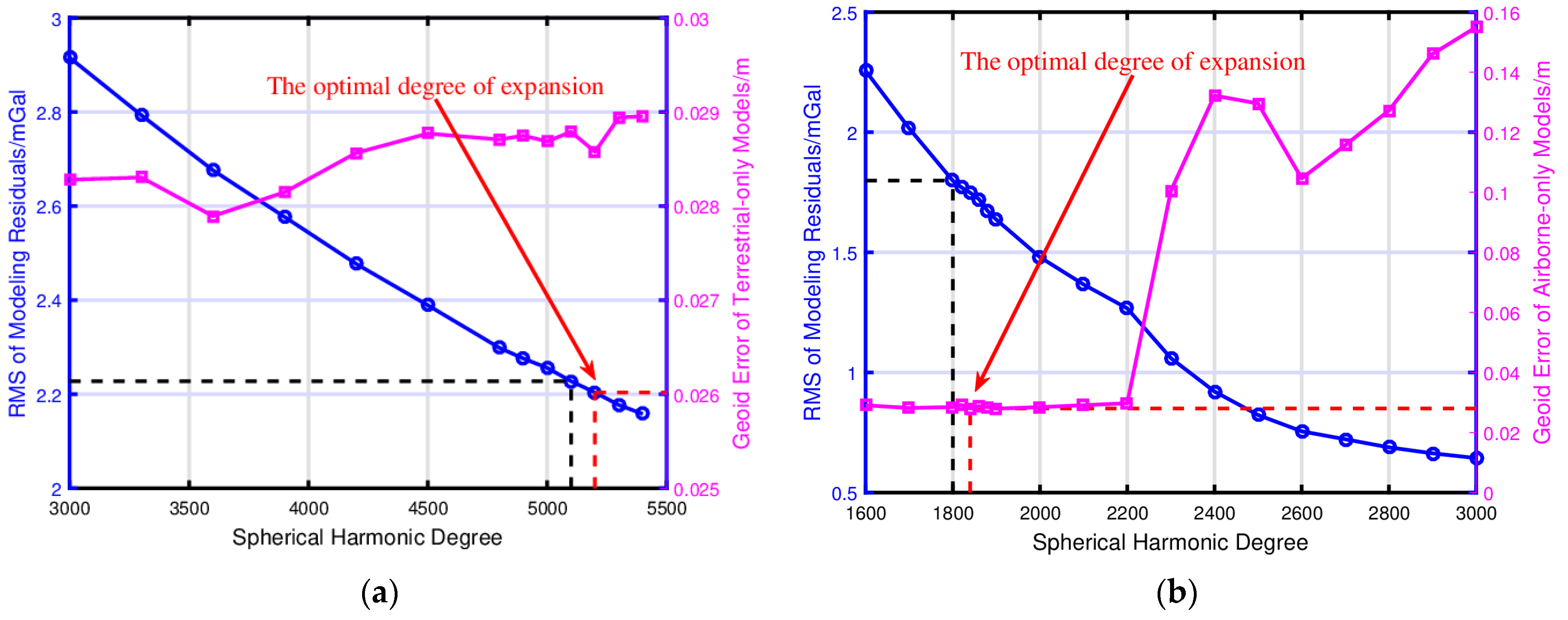
The determination of the optimal expansion degree of terrestrial and airborne gravity data is conducted using the residual and a priori accuracy comparative analysis method. Figure 5 illustrates the procedure to determine the optimal expansion degree of the gravity data. To fully demonstrate the differences caused by the different expansion degrees of SRBFs, the STD values of the geoid height differences between each model and GSVS17 are also calculated. Figure 5a shows that a search range of 3000 to 5400, with a step size of 300, is selected for the terrestrial gravity data in Step 1. For the airborne gravity data, a search range of 1600 to 3000, with a step size of 100, is chosen. When the expansion degrees of the terrestrial and airborne data are 5100 and 1800, respectively, the RMS values of the residuals closely match the a priori accuracy of the gravity data. Hence, these degrees are set as the initial values of expansion for the terrestrial and airborne gravity data (depicted by the black line in Figure 5a,b). Then, in Step 2, smaller search intervals of 4800 to 5400 (with a step size of 100) and of 1800 to 1850 (with a step size of 10) are selected for the terrestrial and airborne data, respectively. When the expansion degrees of the terrestrial and airborne data are 5200 and 1840, respectively, the geoid height differences reach their minimum values (depicted by the red lines in Figure 5a,b).
In addition, as shown in Figure 5, although the residuals of the gravity disturbances decrease with increasing expansion degree, the corresponding geoid accuracy does not exhibit the same trend. In fact, the increase in the expansion degree only improves the agreement between the recovered signal and the original signal, but it can also lead to overfitting of the input gravity data when the expansion degree exceeds the optimal expansion degree of the SRBFs. Thus, the quality of the geoid does not always improve with increasing expansion degree. Additionally, the RMS value of the geoid height differences for airborne gravity data rapidly increases after the expansion degree surpasses 2200, whereas the corresponding change for terrestrial gravity data is not as significant. This indicates that the expansion degree of airborne gravity data may be more sensitive than that of terrestrial gravity data. In addition, according to Equation (15), the spherical harmonic degree of airborne gravity data is approximately 1530, whereas the optimal degree detected in our study is 1840. The resolution of the airborne data explored in this study is approximately 10.6 km, which is smaller than that of the NGS at 12.9 km. However, in terms of the STD of the combined geoid model with respect to GSVS17 (Table 2), the resolution determined for the airborne data in this study seems to be more reliable than the aforementioned approach.
5. Evaluation of the Combined Solution
In this section, we compute two sets of output gravity functionals. The first is the geoid heights at the GSVS17 benchmarks, at which fourteen groups have provided geoid height results. The second is a grid model from 36 to 39 and −109 to −103 with a resolution of . Fourteen groups have provided the geoid height grid model, and the comparison between our models and the mean of all the models is given.
5.1. Comparison to Models with Different Expanding Degrees of SRBFs
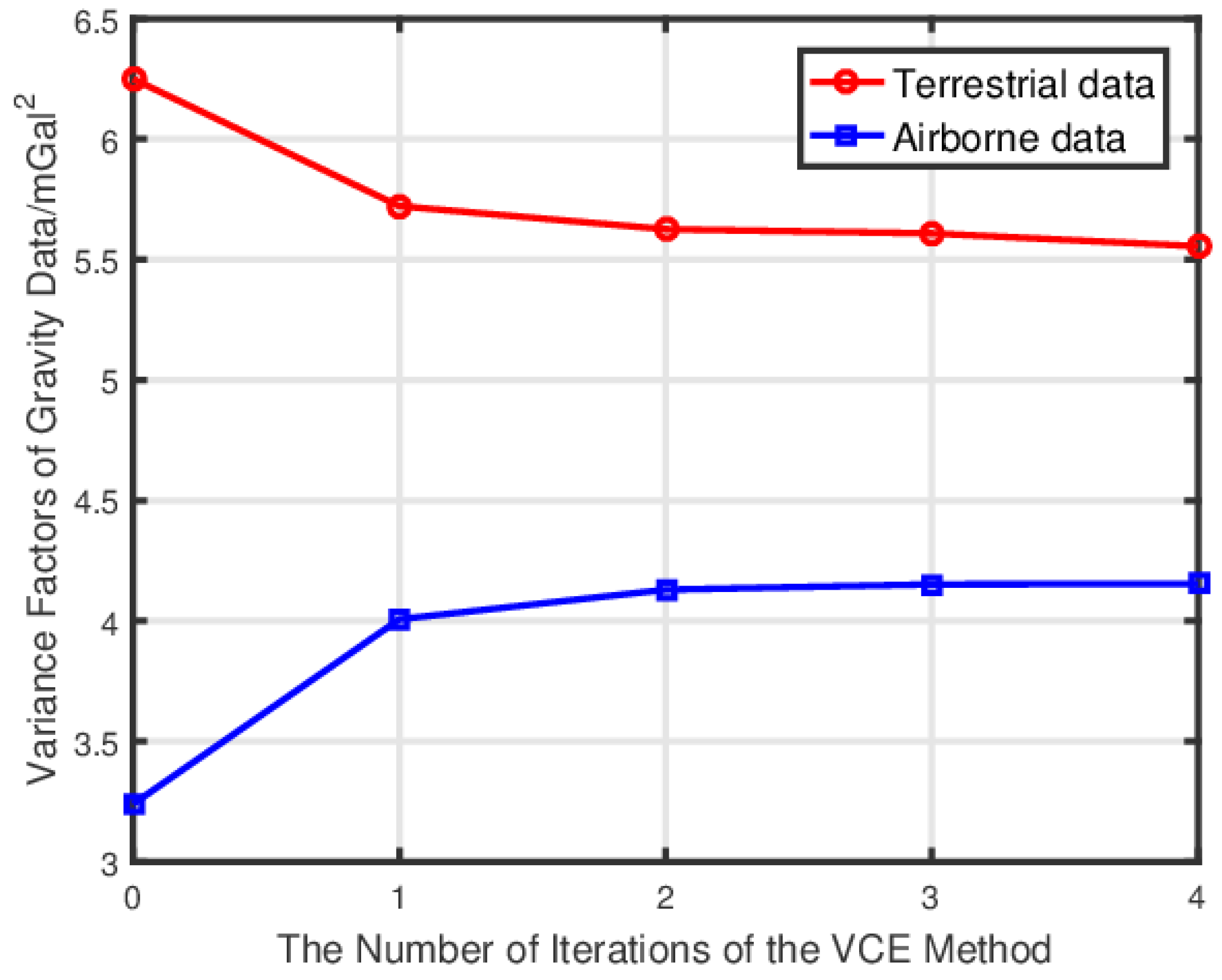
According to Equation (6), there are two variables that need to be determined: the relative weight between the two types of observations and the regularization parameter . Both of these variables are determined through the VCE method, which is an iterative process to estimate the variance factors of different observation types and the prior information. Figure 6 illustrates how the variance factors of the gravity data change during the iteration process.
As seen from Figure 6, the iteration starts with the initial values of , , and , and, after approximately four iterations, the variance factors tend to stabilize, and convergence is reached. The result of the finally obtained variance factors is , , and , respectively. The relative weight between the airborne data and the terrestrial data is approximately 1.34:1, and the regularization parameter is approximately 4752 upon converting mGal to (). Notably, this result differs from that of Liu et al., who obtained variance factors of , , and . Such a result is possible if both the terrestrial and airborne gravity data are expanded to the same higher degree of 5600. Since the standard deviation of the residual airborne gravity data is small, the fitting effect is definitely better than that of terrestrial gravity data. However, it should be noted that the estimated variance factors actually represent the quality of the least squares fit rather than the accuracy of the data themselves.
To assess how our geoid model benefits from the residual and a priori accuracy comparative analysis method, our optimal computed model is compared to the model obtained with different expansion degrees of gravity data. Each model is then compared to the GSVS17 validation data, and the geoid height differences between the models and the GSVS17 validation data are recorded in Table 2.
The results reveal that the geoid models that are obtained with , and (Model I) and , and (Model III) for both terrestrial and airborne gravity data perform the worst, with an STD value of 3.1 cm. However, when the minimum degree of expansion is 720 (Models II and IV), the STD is reduced to 2.6 cm. This suggests that the accuracy of the XGM2016 model up to a degree of 719 is higher than the residual components of the gravity data. Consequently, including the residual signals from degrees 0 to 719 does not contribute to improving the quality of the geoid model. This finding highlights the importance of considering the minimum expansion degree in regional gravity field modeling based on SRBFs. We note that this factor has often been overlooked in previous studies.
The optimal model is Model VI, which is obtained with , , and . When compared to the GSVS17 validation data, the geoid height differences have an STD value of approximately 2.3 cm, which is the smallest among all six selected models (Table 2). The improved performance of Model VI can be attributed to the introduction of the residual and a priori accuracy comparative analysis method, as well as the special treatment of the minimum expansion degree of the SRBFs. Comparing Model VI to Model II and Model V, which have the same expansion degree of terrestrial data but different expansion degrees of airborne data, we find that Model II has an STD of 2.6 cm, while Model V has an STD of 2.5 cm, which are increased by 3 mm and 2 mm, respectively, compared to the STD value of Model VI. Therefore, when aiming at constructing a geoid model with accuracy of 1 cm, it is necessary to consider the potential impact of different expansion degrees of the gravity data.
5.2. GSVS17 Comparisons
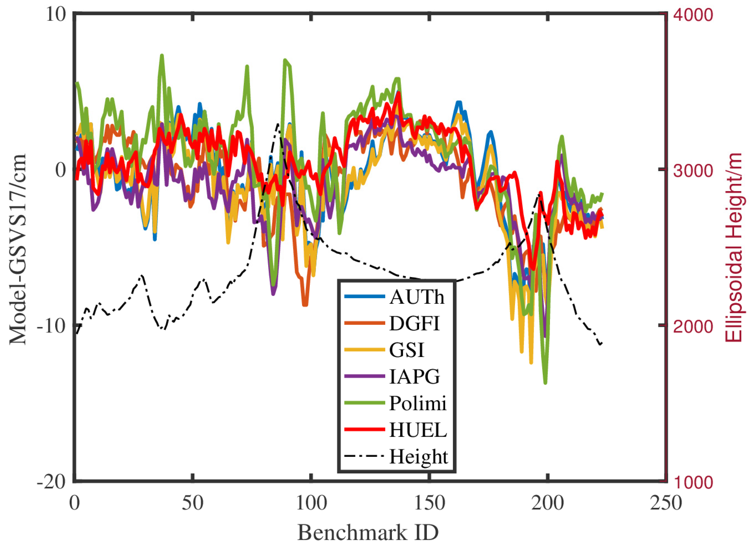
To further evaluate the quality of the optimal geoid model (hereinafter referred to as ColSRBF2023), five geoid models are downloaded from the International Service for the Geoid (ISG). The five models are ColFFTW2020 from Aristotle University of Thessaloniki (AUTh), ColSRBF2019 from the Deutsches Geodätisches Forschungsinstitut (DGFI), ColUNBSH2019 from the Geospatial Information Authority of Japan (GSI), ColRLSC2019 from the Institute for Astronomical and Physical Geodesy (IAPG), and ColWLSC2020 from the Politecnico di Milano (Polimi). The reason for choosing these five models is that they all follow the same RCR procedure. For example, they all use the same reference gravity field model (XGM2016 up to degree 719) and the same methods for removing the topographic effects. Therefore, the above models can better reflect the differences caused by different modeling methods. Importantly, there is a bias of approximately 87 cm between the geopotential value of the reference level and that defined by the NAVD88 datum, which is tied to the tide gauge at Rimouski [53]. This bias has been subtracted in the comparison. Figure 7 shows the geoid height differences of each model along the GSVS17 profile, and Table 3 lists the statistics of the geoid height differences.
Figure 7 shows that the differences between each model and GSVS17 generally follow a similar trend. The STD values of the geoid height differences range from 2.3 cm to 3.9 cm, as listed in Table 3. The model with the smallest STD value is ColSRBF2023, which has a value of approximately 2.3 cm. Table 3 also provides the range of geoid height differences for each model relative to GSVS17. The ranges of differences change from 11.3 cm for the ColSRBF2023 model to 22.8 cm for ColWLSC2020, with an average value of 15.7 cm. These values are quite significant considering the target accuracy of 1 cm for geoid modeling. However, considering the uneven distribution of observations, the result is still quite satisfactory.
In addition, as shown in Figure 7, the differences are clear around the point numbers (Nos.) of 100 and 200, with maximum and minimum deviations of 7.9 cm and −14.9 cm, respectively. This may be attributed to the scarcity of terrestrial gravity data in this section (see Figure 1). Notably, around Nos. 100 and 200, the terrain changes are more significant, and the ColSRBF2023 model is significantly improved compared with the other five models, which indicates the effectiveness of the residual and a priori accuracy comparative analysis method proposed in this study.
5.3. Area Comparison of Geoid Grids
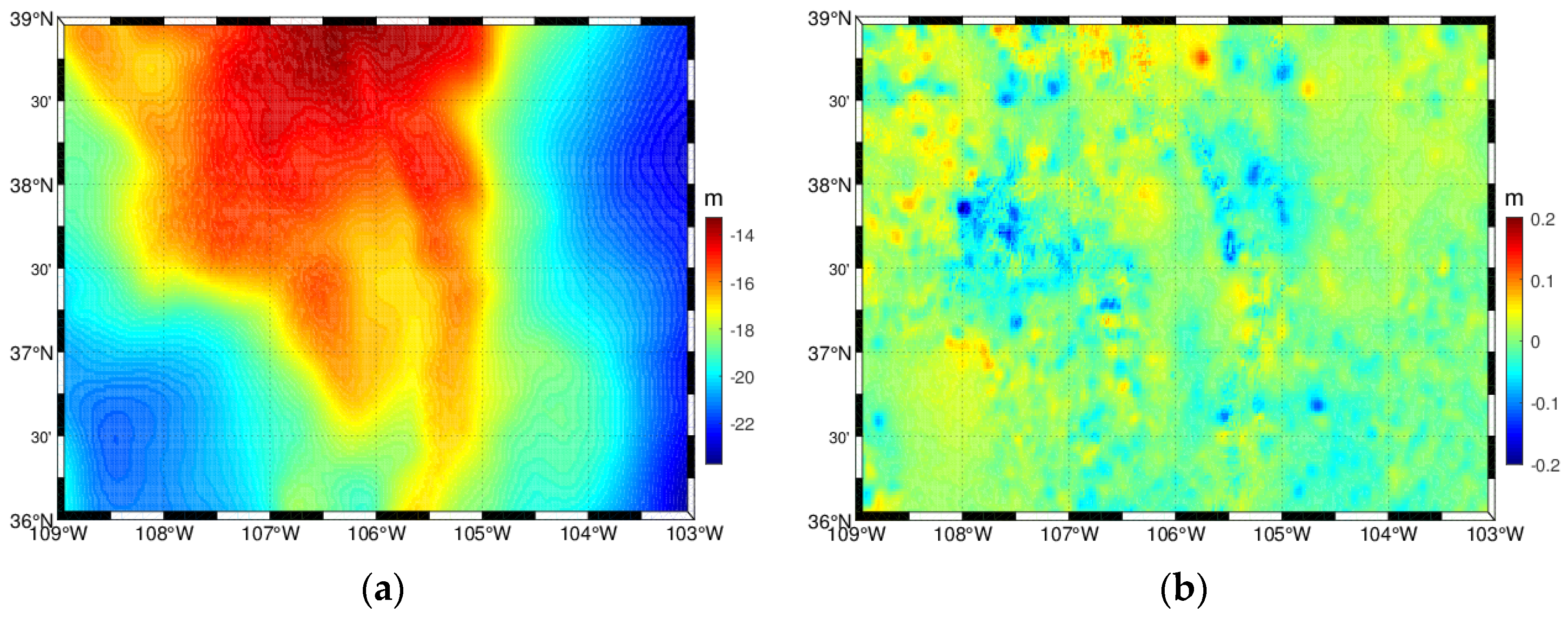
Since GSVS17 is located in a relatively flat area, comparison with GSVS17 may not reflect the quality of the model for the entire study area. Therefore, we employ the average value of the geoid grid models submitted to ISG as a calibration model to better evaluate the quality of ColSRBF2023. Figure 8a visualizes the geoid model of ColSRBF2023 for the whole target area , with a grid interval of , and Figure 8b shows the geoid height differences with respect to the calibration geoid model. Table 4 provides the statistics of the geoid height differences.
From Figure 8b, we can see that large differences are mainly concentrated on the east and west sides of the target area (dark blue and dark red blocks in Figure 8b). These areas are characterized by drastic elevation variations and sparse distributions of gravity data, highlighting the importance of the gravity data’s density and quality. In other areas (yellow and light blue regions in Figure 8b), the differences are relatively small, generally not exceeding ±5 cm. Furthermore, in terms of the RMS of the geoid height differences, ColSRBF2023 has a value of 2.4 cm, while the other three models have values of 3.0 cm, 3.0 cm, and 2.9 cm. ColSRBF2023 has the smallest RMS value among all the compared models. Additionally, the model with the largest range of geoid height differences is ColUNBSH2019 (GSI), reaching 48.1 cm. ColSRBF2023 performs slightly better, with a range of 31.8 cm (Table 4). The overall average range of geoid height differences for all models is 41.8 cm, which reflects the significant challenge in achieving 1 cm accuracy in geoid modeling in mountainous areas.
In general, the best model in this study is the combined geoid model ColSRBF2023 with , , and (Table 2). The STD and RMS values of the geoid height differences with respect to the validation model are both 2.4 cm. The distribution of the difference is relatively uniform, which indicates the effectiveness of the residual and a priori accuracy comparative analysis method and the treatment of the minimum degree of expansion of SRBFs.
6. Summary and Outlook
After the earlier work undertaken by Schmidt et al., Eicker, and Klees et al., SRBFs have been widely used for regional gravity field modeling in the last two decades. In this study, we combine terrestrial gravity data, airborne gravity data, GGMs, and topographic models to calculate a high-resolution geoid model in Colorado based on band-limited SRBFs. Detailed explanations are given regarding the determination of the optimal expansion degree of gravity data: the optimal maximum expansion degree of terrestrial and airborne gravity data and the minimum expansion degree of gravity data. The main conclusions are as follows.
(1) The residual and a priori accuracy comparative analysis method can be an effective approach to determining the optimal expansion degree of gravity data. Using this method, the optimal expansion degrees of terrestrial and airborne data are determined to be 5200 and 1840, respectively. Additionally, the STD value of our optimal geoid model ColSRBF2023 with respect to GSVS17 data was 2.3 cm, which is smaller than all the other geoid models in this study.
(2) The minimum degree of expansion of the gravity data also plays a role in the modeling result. If the expansion degree is not properly determined, it can lead to geoid height differences of ~5 mm. This highlights the importance of accurately determining the minimum expansion degree of gravity data.
(3) Compared with ColSRBF2019, ColUNBSH2019, ColRLSC2019, and ColWLSC2020 submitted to ISG by different institutions, the ColSRBF2023 model showed a reduction in the STD value of approximately 0.2–1.6 cm with respect to the GSVS17 data.
(4) Comparisons are also made with the mean geoid model of ISG. ColSRBF2023 for the whole target area delivers an STD value of 2.4 cm, which is also a small value for all participants. Moreover, there is favorable agreement between the STD value with respect to the area mean solutions and the STD with respect to the GSVS17 GPS/leveling data, which shows the reliability of our geoid model ColSRBF2023 to a certain extent.
Overall, in this study, we aimed to enhance the quality of the geoid model in Colorado using band-limited SRBFs. To achieve this, the investigation and determination of the optimal expansion degrees for both terrestrial and airborne gravity data were conducted. The optimal geoid model was obtained when the maximum expansion degrees for terrestrial and airborne gravity data were determined to be 5200 and 1840, respectively, while the minimum expansion degrees for both data types were set to 720. The study demonstrated the significance of accurately determining the spectral information of gravity data, particularly in rugged areas. In future studies, we plan to perform further analyses of the remaining error sources in the determination of geoid models based on band-limited SRBFs, including the effect of the cutoff degree of the GGM, topographic reductions, and different approaches to handling airborne data, thereby furthering our contribution to the 1 cm geoid experiment of Colorado.
Author Contributions
Conceptualization, Z.M.; methodology, Z.M.; funding acquisition and project administration, Z.M. and J.L.; software, Z.M.; supervision and validation, M.Y.; writing—original draft, Z.M.; writing—review and editing, J.L. All authors have read and agreed to the published version of the manuscript.
Funding
This research was funded by the National Natural Science Foundation of China, grant number 42104087, and the Natural Science Foundation of Henan Province, grant number 232300421401.
Data Availability Statement
The terrestrial gravity data, airborne gravity data, and point file of the GSVS17 GPS/leveling data used in this study were provided by the National Geodetic Survey for the ‘1 cm Geoid Experiment’. The airborne gravity data are freely available at https://www.ngs.noaa.gov/GRAV-D/data_products.shtml, accessed on 15 April 2023. All data for this paper are properly cited and referred to in the reference list.
Acknowledgments
The authors are very grateful to the NGS, the ISG, and the ICGEM for providing gravity, GPS/leveling, geoid and GGM data.
Conflicts of Interest
The authors declare no conflict of interest.
References
- Varga, M.; Pitoňák, M.; Novák, P.; Bašić, T. Contribution of GRAV-D airborne gravity to improvement of regional gravimetric geoid modelling in Colorado, USA. J. Geod. 2021, 95, 53. [Google Scholar] [CrossRef]
- Forsberg, R.; Tscherning, C.C. The use of height data in gravity field approximation by collocation. J. Geophys. Res. 1981, 86, 7843–7854. [Google Scholar] [CrossRef]
- Novák, P.; Heck, B. Downward continuation and geoid determination based on band-limited airborne gravity data. J. Geod. 2002, 76, 269–278. [Google Scholar] [CrossRef]
- Hwang, C.; Hsiao, Y.S.; Shih, H.C.; Yang, M.; Chen, K.H.; Forsberg, R.; Olesen, A.V. Geodetic and geophysical results from a Taiwan airborne gravity survey: Data reduction and accuracy assessment. J. Geophys. Res. 2007, 112, B04407. [Google Scholar] [CrossRef]
- Willberg, M.; Zingerle, P.; Pail, R. Integration of airborne gravimetry data filtering into residual least-squares collocation: Example from the 1 cm geoid experiment. J. Geod. 2020, 94, 75. [Google Scholar] [CrossRef]
- Li, X. Using radial basis functions in airborne gravimetry for local geoid improvement. J. Geod. 2017, 92, 471–485. [Google Scholar] [CrossRef]
- Tscherning, C.C. Geoid determination by 3D least-squares collocation. In Geoid Determination; Sansò, F., Sideris, M.G., Eds.; Lecture Notes in earth System Sciences; Springer: Berlin, Germany, 2013; Volume 110, pp. 311–336. [Google Scholar] [CrossRef]
- Kern, M.; Schwarz, K.K.P.P.; Sneeuw, N. A study on the combination of satellite, airborne, and terrestrial gravity data. J. Geod. 2003, 77, 217–225. [Google Scholar] [CrossRef]
- Shih, H.C.; Hwang, C.; Barriot, J.P.; Mouyen, M.; Corréia, P.; Lequeux, D.; Sichoix, L. High-resolution gravity and geoid models in Tahiti obtained from new airborne and land gravity observations: Data fusion by spectral combination. Earth Planets Space 2015, 67, 124. [Google Scholar] [CrossRef]
- Simons, F.J.; Dahlen, F.A. Spherical Slepian functions and the polar gap in geodesy. Geophys. J. Int. 2006, 166, 1039–1061. [Google Scholar] [CrossRef]
- Wittwer, T. Regional Gravity Field Modelling with Radial Basis Functions; Delft University of Technology: Delft, The Netherlands, 2009; Available online: https://ncgeo.nl/downloads/72Wittwer.pdf (accessed on 12 September 2014).
- Schmidt, M.; Fengler, M.; Mayer-Gürr, T.; Eicker, A.; Kusche, J.; Sánchez, L.; Han, S.-C. Regional gravity modeling in terms of spherical base functions. J. Geod. 2007, 81, 17–38. [Google Scholar] [CrossRef]
- Klees, R.; Tenzer, R.; Prutkin, I.; Wittwer, T. A data-driven approach to local gravity field modelling using spherical radial basis functions. J. Geod. 2008, 82, 457–471. [Google Scholar] [CrossRef]
- Eicker, A. Gravity Field Refinement by Radial Basis Functions from In-Situ Satellite Data; Universität Bonn: Bonn, Germany, 2008. [Google Scholar]
- Bentel, K.; Schmidt, M.; Denby, C.R. Artifacts in regional gravity representations with spherical radial basis functions. J. Geod. Sci. 2013, 3, 173–187. [Google Scholar] [CrossRef]
- Lieb, V.; Schmidt, M.; Dettmering, D.; Börger, K. Combination of various observation techniques for regional modeling of the gravity field. J. Geophys. Res. Solid Earth 2016, 121, 3825–3845. [Google Scholar] [CrossRef]
- Bucha, B.; Janák, J.; Papčo, J.; Bezděk, A. High-resolution regional gravity field modelling in a mountainous area from terrestrial gravity data. Geophys. J. Int. 2016, 207, 949–966. [Google Scholar] [CrossRef]
- Klees, R.; Slobbe, D.; Farahani, H. A methodology for least-squares local quasi-geoid modelling using a noisy satellite-only gravity field model. J. Geod. 2018, 92, 431–442. [Google Scholar] [CrossRef]
- Slobbe, C.; Klees, R.; Farahani, H.H.; Huisman, L.; Alberts, B.; Voet, P.; De Doncker, F. The Impact of Noise in a GRACE/GOCE Global Gravity Model on a Local Quasi-Geoid. J. Geophys. Res. Solid Earth 2019, 124, 3219–3237. [Google Scholar] [CrossRef]
- Liu, Q.; Schmidt, M.; Sánchez, L.; Willberg, M. Regional gravity field refinement for (quasi-) geoid determination based on spherical radial basis functions in Colorado. J. Geod. 2020, 94, 99. [Google Scholar] [CrossRef]
- Liu, Y.; Lou, L. Unified land–ocean quasi-geoid computation from heterogeneous data sets based on radial basis functions. Remote Sens. 2022, 14, 3015. [Google Scholar] [CrossRef]
- Freeden, W.; Gervens, T.; Schreiner, M. Constructive Approximation on the Sphere with Applications to Geomathematics; Oxford University Press on Demand: New York, NY, USA, 1998. [Google Scholar]
- Heiskanen, W.A.; Moritz, H. Physical Geodesy; W.H. Freeman and Company: San Francisco, CA, USA, 1967. [Google Scholar]
- Koch, K.-R.; Kusche, J. Regularization of geopotential determination from satellite data by variance components. J. Geod. 2002, 76, 259–268. [Google Scholar] [CrossRef]
- Hutchinson, M.F. A stochastic estimator of the trace of the influence matrix for Laplacian smoothing splines. Commun. Stat.-Simul. Comput. 1990, 19, 433–450. [Google Scholar] [CrossRef]
- Flury, J.; Rummel, R. On the geoid–quasigeoid separation in mountain areas. J. Geod. 2009, 83, 829–847. [Google Scholar] [CrossRef]
- Wang, Y.M.; Li, X.; Ahlgren, K.; Krcmaric, J. Colorado geoid modeling at the US National Geodetic Survey. J. Geod. 2020, 94, 106. [Google Scholar] [CrossRef]
- Grigoriadis, V.N.; Vergos, G.S.; Barzaghi, R.; Carrion, D.; Koç, Ö. Collocation and FFT-based geoid estimation within the Colorado 1 cm geoid experiment. J. Geod. 2021, 95, 52. [Google Scholar] [CrossRef]
- Wang, Y.M.; Holmes, S.; Li, X.; Ahlgren, K. NGS Annual Experimental Geoid Models–xGEOID17: What Is New and the Results; IAG-IASPEI: Kobe, Japan, 2017. [Google Scholar]
- GRAV-D Team. Gravity for the Redefinition of the American Vertical Datum (GRAV-D) Project, Airborne Gravity Data; Block MS05. 2017. Available online: http://www.ngs.noaa.gov/GRAV-D/data_MS05.shtml (accessed on 15 November 2022).
- van Westrum, D.; Ahlgren, K.; Hirt, C.; Guillaume, S. A Geoid Slope Validation Survey (2017) in the rugged terrain of Colorado, USA. J. Geod. 2021, 95, 9. [Google Scholar] [CrossRef]
- Rebischung, P.; Griffiths, J.; Ray, J.; Schmid, R.; Collilieux, X.; Garayt, B. IGS08: The IGS realization of ITRF2008. GPS Solut. 2012, 16, 483–494. [Google Scholar] [CrossRef]
- Moritz, H. Geodetic Reference System 1980. J. Geod. 2000, 74, 128–133. [Google Scholar] [CrossRef]
- NGS. Technical Details for GEOID18B. 2018. Available online: https://geodesy.noaa.gov/GEOID/GEOID18.shtml (accessed on 12 May 2023).
- Torge, W. Gravimetry; Walter de Gruyter: Berlin, Germany, 1989. [Google Scholar]
- Pavlis, N.K.; Holmes, S.A.; Kenyon, S.C.; Factor, J.K. The Development and Evaluation of the Earth Gravitational Model 2008 (EGM2008). J. Geophys. Res. 2012, 117, B04406. [Google Scholar] [CrossRef]
- Zingerle, P.; Pail, R.; Gruber, T.; Oikonomidou, X. The Experimental Gravity Field Model XGM2019e; GFZ: Potsdam, Germany, 2019. [Google Scholar]
- Liang, W.; Li, J.; Xu, X.; Zhang, S.; Zhao, Y. A High-Resolution Earth’s Gravity Field Model SGG-UGM-2 from GOCE, GRACE, Satellite Altimetry, and EGM2008. Engineering 2020, 6, 860–878. [Google Scholar] [CrossRef]
- Pail, R.; Fecher, T.; Barnes, D.; Factor, J.F.; Holmes, S.A.; Gruber, T.; Zingerle, P. Short Note: The Experimental Geopotential Model XGM2016. J. Geod. 2018, 92, 443–451. [Google Scholar] [CrossRef]
- Gilardoni, M.; Reguzzoni, M.; Sampietro, D. GECO: A Global Gravity Model by Locally Combining GOCE Data and EGM2008. Stud. Geophys. Geod. 2015, 60, 228–247. [Google Scholar] [CrossRef]
- Pail, R.; Bruinsma, S.; Migliaccio, F.; Förste, C.; Goiginger, H.; Schuh, W.-D.; Höck, E.; Reguzzoni, M.; Brockmann, J.M.; Abrikosov, O.; et al. First GOCE Gravity Field Models Derived by Three Different Approaches. J. Geod. 2011, 85, 819–843. [Google Scholar] [CrossRef]
- Wu, Y.; He, X.; Luo, Z.; Shi, H. An Assessment of Recently Released High-Degree Global Geopotential Models Based on Heterogeneous Geodetic and Ocean Data. Front. Earth Sci. 2021, 9, 749611. [Google Scholar] [CrossRef]
- Rexer, M.; Hirt, C.; Claessens, S.; Tenzer, R. Layer-based modelling of the Earth’s gravitational potential up to 10-km scale in spherical harmonics in spherical and ellipsoidal approximation. Surv. Geophys. 2016, 37, 1035–1074. [Google Scholar] [CrossRef]
- Hirt, C.; Kuhn, M.; Claessens, S.; Pail, R.; Seitz, K.; Gruber, T. Study of the Earth’s short-scale gravity field using the ERTM2160 gravity model. Comput. Geosci. 2014, 73, 71–80. [Google Scholar] [CrossRef]
- Freeden, W.; Schneider, F. An integrated wavelet concept of physical geodesy. J. Geod. 1998, 72, 259–281. [Google Scholar] [CrossRef]
- Reuter, R. Über Integralformeln der Einheitssphäre und Harmonische Splinefunktionen; RWTH Aachen University: Aachen, Germany, 1982. [Google Scholar]
- Naeimi, M.; Flury, J.; Brieden, P. On the regularization of regional gravity field solutions in spherical radial base functions. Geophys. J. Int. 2015, 202, 1041–1053. [Google Scholar] [CrossRef]
- Naeimi, M. Inversion of Satellite Gravity Data Using Spherical Radial Base Functions; Leibniz Universität Hannover: Hannover, Germany, 2013; Available online: https://dgk.badw.de/fileadmin/user_upload/Files/DGK/docs/c-711.pdf (accessed on 20 July 2016).
- Saleh, J.; Li, X.; Wang, Y.; Roman, D.; Smith, D. Error analysis of the NGS’ surface gravity database. J. Geod. 2013, 87, 203–221. [Google Scholar] [CrossRef]
- Işık, M.S.; Erol, B.; Erol, S.; Sakil, F.F. High-resolution geoid modeling using least squares modification of stokes and hotine formulas in Colorado. J. Geod. 2021, 95, 49. [Google Scholar] [CrossRef]
- Jiang, T.; Dang, Y.M.; Zhang, C.Y. Gravimetric geoid modeling from the combination of satellite gravity model, terrestrial and airborne gravity data: A case study in the mountainous area, Colorado. Earth Planets Space 2020, 72, 189. [Google Scholar] [CrossRef]
- Wang, Y.M.; Sánchez, L.; Ågren, J.; Huang, J.; Forsberg, R.; Abd-Elmotaal, H.A.; Ahlgren, K.; Barzaghi, R.; Bašić, T.; Carrion, D.; et al. Colorado geoid computation experiment: Overview and summary. J. Geod. 2021, 95, 127. [Google Scholar] [CrossRef]
- Zilkoski, D.B.; Richards, J.H.; Young, G.M. Results of the general adjustment of the North American Vertical Datum of 1988. Surv. Land. Inf. Syst. 1992, 52, 133–149. [Google Scholar]
Figure 1.
(a) Topographic heights in the Colorado area. (b) Datasets: terrestrial gravity data (blue), duplicated points (purple) and airborne gravity observations (orange), GSVS17 benchmarks (red), and the target area (black rectangle).
Figure 1.
(a) Topographic heights in the Colorado area. (b) Datasets: terrestrial gravity data (blue), duplicated points (purple) and airborne gravity observations (orange), GSVS17 benchmarks (red), and the target area (black rectangle).

Figure 2.
Cumulative geoid errors of different GGMs.

Figure 3.
(a,b) Gravity observations (); (c,d) remaining parts after both the GGM and topographic reduction () for the terrestrial data (left column) and airborne data (right column).
Figure 3.
(a,b) Gravity observations (); (c,d) remaining parts after both the GGM and topographic reduction () for the terrestrial data (left column) and airborne data (right column).

Figure 4.
The extensions of the computation area
(green color), observation area , and target area .
Figure 4.
The extensions of the computation area
(green color), observation area , and target area .

Figure 5.
Residual and a priori accuracy comparative analysis method used to find the optimal expansion degree of the terrestrial gravity data (a) and airborne gravity data (b). Blue: RMS value of the modeling residuals (mGal). Purple: Geoid accuracy of the terrestrial-only and airborne-only models (m).Black dot line: initial degree of expansion determined by Step 1. Red dot line: the optimal degree of expansion determined by Step 2.

Figure 6.
Changes in variance factors of gravity data with the number of iterations.

Figure 7.
Geoid height differences on the GSVS17 benchmarks (). Here, 87 cm is subtracted from the models.
Figure 7.
Geoid height differences on the GSVS17 benchmarks (). Here, 87 cm is subtracted from the models.

Figure 8.
(a) The distributions of geoid heights of ColSRBF2023 at the grid. (b) The distributions of differences between ColSRBF2023 and the mean geoid model at the grid.
Figure 8.
(a) The distributions of geoid heights of ColSRBF2023 at the grid. (b) The distributions of differences between ColSRBF2023 and the mean geoid model at the grid.


Table 1.
Statistics of the gravity observations.
| Data | Max (mGal) | Min (mGal) | Mean (mGal) | STD (mGal) |
|---|---|---|---|---|
| 207.88 | −146.36 | 0.35 | 38.72 | |
| 137.40 | −151.34 | −5.64 | 22.40 | |
| 75.328 | −135.86 | 0.76 | 6.90 | |
| 123.24 | −43.88 | 7.33 | 29.56 | |
| 68.25 | −43.06 | 0.06 | 8.16 | |
| 19.01 | −18.97 | 0.10 | 3.35 |
Table 2.
Comparison of the combined models based on different expansion degrees of SRBFs.
| Model | Max (cm) | Min (cm) | Mean (cm) | STD (cm) | |||
|---|---|---|---|---|---|---|---|
| Model I | 5600 | 5600 | 0 | 93.6 | 79.6 | 88.6 | 3.1 |
| Model II | 5600 | 5600 | 720 | 92.0 | 80.8 | 87.1 | 2.6 |
| Model III | 5200 | 5200 | 0 | 94.0 | 80.5 | 89.1 | 3.1 |
| Model IV | 5200 | 5200 | 720 | 91.8 | 81.1 | 87.0 | 2.6 |
| Model V | 5200 | 1530 | 720 | 91.9 | 80.4 | 87.2 | 2.5 |
| Model VI | 5200 | 1840 | 720 | 91.9 | 80.0 | 87.3 | 2.3 |
Table 3.
Statistics of geoid height differences on the GSVS17 benchmarks (). Here, 87 cm is subtracted from the models.
Table 3.
Statistics of geoid height differences on the GSVS17 benchmarks (). Here, 87 cm is subtracted from the models.
| Model | Institution | Max (cm) | Min (cm) | Mean (cm) | STD (cm) | Range (cm) |
|---|---|---|---|---|---|---|
| ColFFTW2020 | AUTh | 3.4 | −10.7 | −1.0 | 2.5 | 14.1 |
| ColSRBF2019 | DGFI | 5.0 | −10.8 | −0.6 | 3.0 | 15.8 |
| ColUNBSH2019 | GSI | 3.8 | −9.6 | −0.7 | 3.2 | 13.4 |
| ColRLSC2019 | IAPG | 4.1 | −12.4 | −0.9 | 3.1 | 16.5 |
| ColWLSC2020 | Polimi | 7.9 | −14.9 | 0.7 | 3.9 | 22.8 |
| ColSRBF2023 | HUEL | 4.9 | −6.4 | 0.3 | 2.3 | 11.3 |
Note: HUEL stands for Henan University of Economics and Law, China.
Table 4.
Statistics of the differences among the individual geoid models and the mean geoid models at the grid.
Table 4.
Statistics of the differences among the individual geoid models and the mean geoid models at the grid.
| Model | Institution | Max (cm) | Min (cm) | Mean (cm) | STD (cm) | RMS (cm) | Range (cm) |
|---|---|---|---|---|---|---|---|
| ColSRBF2019 | DGFI | 11.7 | −34.0 | −0.9 | 2.8 | 3.0 | 45.7 |
| ColUNBSH2019 | GSI | 24.1 | −24.0 | 0. 3 | 3.0 | 3.0 | 48.1 |
| ColRLSC2019 | IAPG | 10.3 | −31.5 | −1.3 | 2.6 | 2.9 | 41.8 |
| ColSRBF2023 | HUEL | 11.9 | −19.9 | 0.1 | 2.4 | 2.4 | 31.8 |
Note: The models of ColFFTW2020 (AUTh) and ColWLSC2020 (Polimi) do not cover the whole study area, so they are not included in the comparison.
Disclaimer/Publisher’s Note: The statements, opinions and data contained in all publications are solely those of the individual author(s) and contributor(s) and not of MDPI and/or the editor(s). MDPI and/or the editor(s) disclaim responsibility for any injury to people or property resulting from any ideas, methods, instructions or products referred to in the content. |
© 2023 by the authors. Licensee MDPI, Basel, Switzerland. This article is an open access article distributed under the terms and conditions of the Creative Commons Attribution (CC BY) license (https://creativecommons.org/licenses/by/4.0/).
Share and Cite
MDPI and ACS Style
Ma, Z.; Yang, M.; Liu, J. Regional Gravity Field Modeling Using Band-Limited SRBFs: A Case Study in Colorado. Remote Sens. 2023, 15, 4515. https://doi.org/10.3390/rs15184515
AMA Style
Ma Z, Yang M, Liu J. Regional Gravity Field Modeling Using Band-Limited SRBFs: A Case Study in Colorado. Remote Sensing. 2023; 15(18):4515. https://doi.org/10.3390/rs15184515
Chicago/Turabian StyleMa, Zhiwei, Meng Yang, and Jie Liu. 2023. "Regional Gravity Field Modeling Using Band-Limited SRBFs: A Case Study in Colorado" Remote Sensing 15, no. 18: 4515. https://doi.org/10.3390/rs15184515
Note that from the first issue of 2016, this journal uses article numbers instead of page numbers. See further details here.