
Integrating Topographic Skeleton into Deep Learning for Terrain Reconstruction from GDEM and Google Earth Image
by
 , and
, and
Kai Chen
1,2,
Chun Wang
2,3,*,
Mingyue Lu
1,
Wen Dai
1,
Jiaxin Fan
4,
Mengqi Li
1 and
Shaohua Lei
5 1
School of Geographical Sciences, Nanjing University of Information Science and Technology, Nanjing 210044, China
2
Key Laboratory of Physical Geographic Information in Anhui Province, Chuzhou 239000, China
3
School of Geographic Information and Tourism, Chuzhou University, Chuzhou 239000, China
4
School of Remote Sensing & Geomatics Engineering, Nanjing University of Information Science and Technology, Nanjing 210044, China
5
State Key Laboratory of Hydrology-Water Resources and Hydraulic Engineering, Nanjing Hydraulic Research Institute, Nanjing 210029, China
*
Author to whom correspondence should be addressed.
Remote Sens. 2023, 15(18), 4490; https://doi.org/10.3390/rs15184490
Submission received: 21 July 2023
/
Revised: 22 August 2023
/
Accepted: 8 September 2023
/
Published: 12 September 2023
(This article belongs to the Special Issue Machine Learning for Multi-Source Remote Sensing Images Analysis)
Abstract
:The topographic skeleton is the primary expression and intuitive understanding of topographic relief. This study integrated a topographic skeleton into deep learning for terrain reconstruction. Firstly, a topographic skeleton, such as valley, ridge, and gully lines, was extracted from a global digital elevation model (GDEM) and Google Earth Image (GEI). Then, the Conditional Generative Adversarial Network (CGAN) was used to learn the elevation sequence information between the topographic skeleton and high-precision 5 m DEMs. Thirdly, different combinations of topographic skeletons extracted from 5 m, 12.5 m, and 30 m DEMs and a 1 m GEI were compared for reconstructing 5 m DEMs. The results show the following: (1) from the perspective of the visual effect, the 5 m DEMs generated with the three combinations (5 m DEM + 1 m GEI, 12.5 m DEM + 1 m GEI, and 30 m DEM + 1 m GEI) were all similar to the original 5 m DEM (reference data), which provides a markedly increased level of terrain detail information when compared to the traditional interpolation methods; (2) from the perspective of elevation accuracy, the 5 m DEMs reconstructed by the three combinations have a high correlation (>0.9) with the reference data, while the vertical accuracy of the 12.5 m DEM + 1 m GEI combination is obviously higher than that of the 30 m DEM + 1 m GEI combination; and (3) from the perspective of topographic factors, the distribution trends of the reconstructed 5 m DEMs are all close to the reference data in terms of the extracted slope and aspect. This study enhances the quality of open-source DEMs and introduces innovative ideas for producing high-precision DEMs. Among the three combinations, we recommend the 12.5 m DEM + 1 m GEI combination for DEM reconstruction due to its relative high accuracy and open access. In regions where a field survey of high-precision DEMs is difficult, open-source DEMs combined with GEI can be used in high-precision DEM reconstruction.
1. Introduction
The terrain is a description of the earth’s surface, encompassing various geomorphic evolutionary processes. Moreover, the terrain reflects major crustal movements (i.e., geological changes) and minor change processes (i.e., soil erosion and water loss) [1,2]. Terrain modeling serves as the foundation for various scientific research and engineering applications. These applications cover several areas, including meteorological analysis, disaster prevention and control, hydrological analysis, crop cultivation, geological analysis, feature construction, military battlefield simulations, and game modeling [3,4,5,6,7,8,9,10]. Over the years, scholars have proposed various terrain modeling approaches, which can be broadly categorized into two types: physical terrain modeling based on field measurements and virtual terrain modeling based on existing information and geological knowledge.
Physical terrain modeling primarily involves traditional geodetic surveying and remote-sensing methods based on field measurements. Elevation values, which simulate the physical terrain, are directly obtained from measuring instruments or from aerospace satellite remote-sensing platforms, unmanned aerial vehicle (UAV) photogrammetry, and Light Detection and Ranging (LIDAR) [11,12,13,14]. Modeling methods based on field measurements are expensive despite their accuracy. For terrain simulation methods based on known information, models are primarily constructed from known terrain and topographic knowledge, including constrained interpolation algorithms and the functionalized terrain modeling method. The former has typical interpolation algorithms, such as inverse distance weighting and cubic convolutional interpolation [15,16,17,18]. Meanwhile, the latter is a technique that uses various surface parameters and input formulas to create terrain output. This method uses fractal algorithms, physical modeling methods, meta-cellular automata, and simulation algorithms utilized in fluid particle systems [19,20,21,22,23]. Modeling methods based on existing data are direct. However, applying the generated terrain to geomorphological simulation is difficult because terrain formation involves geomorphic development processes and geographic laws. Describing surface details and reflecting geomorphic development processes using a single-function approach are also complicated.
The difficulty in reconstructing terrain based on known information and topographic knowledge lies in the complexity of the elevation pattern of the terrain slope; thus, establishing a global terrain model with certain formulas or constraints is difficult [24]. One of the most effective methods for dealing with big data, deep learning, can autonomously mine learning features for terrain modeling [25]. Consequently, deep-learning-based terrain modeling has been developing, and preliminary research has been conducted on Image Super-Resolution and image generation techniques. However, this direct scale-down method lacks theoretical support and is inappropriate for complex terrain, demonstrating poor interpretation, low stability, and limited model applicability based on the experience of some scholars [26,27]. The image generation method conceptualizes the DEM in a regular grid format as an image generation problem with feature elements, and the terrain features significantly influence the topography. The CGAN is a prevalent deep-learning technique for good-quality image generation [28,29]. Therefore, numerous researchers [30,31,32] introduced a CGAN training method by utilizing high-precision DEM-extracted terrain elements, which later created DEMs according to the trained networks. However, certain drawbacks are still evident despite the modern technique used in this approach for terrain modeling. On the one hand, obtaining a high-precision DEM is difficult in mountainous and remote areas, and the dependence of this method on high-precision DEMs limits its applicability. On the other hand, training to generate the corresponding high-precision DEM has minimal practical importance due to the already existing high-precision DEMs.
Acquiring coarse-resolution DEM and image data for a large spatial extent is easy. Meanwhile, a high-resolution DEM can be accessible through UAV photogrammetry. In such cases, utilizing the available topographic information and accurate data from a sub-region to train a model that can reconstruct elevations at the same geomorphic development features in other parts is scientifically and practically valuable. A group of scholars utilized global open-source Global Digital Elevation Models (GDEMs), including ALOS (Advanced Land Observing Satellite) DEM, ASTER (Advanced Spaceborne Thermal Emission and Reflection Radiometer) DEM, SRTM (Shuttle Radar Topography Mission) DEM, and other GDEMs, due to their extensive coverage [11,33,34,35,36]. This study is valuable because it employs the similarities of valley and ridge lines extracted by different DEM resolutions, the high-resolution property of remote-sensing images, and the advancement of CGAN technology [37]. The objectives of this study were as follows: (1) integrate topo- graphic skeleton lines into deep learning for terrain reconstruction from Google Earth Image and GDEM and (2) verify the effectiveness of two global open-source GDEMs and Google Earth Image for producing higher-resolution DEMs. This study also examined the potential of multiple datasets in creating a 5 m high-precision DEM, enabling the prompt creation of high-precision terrain modeling for various circumstances, such as engineering constructions, environmental assessments, and battlefield environment simulations, using the pre-existing datasets.
2. Method
2.1. Basic Ideas
Topographic skeletons, such as ridges, valleys, and gully lines, are derived from the terrain, representing the surface height and undulation, and are the basis for generating simulated terrain using deep-learning algorithms. A scale effect exists in a DEM, wherein different-resolution DEMs are not only similar in expressing the spatial location of mountains and river valleys but also the same length as the same catchment area [38,39,40]. Therefore, there is a certain conversion rule between the ridge and valley lines of different resolution DEMs. The gully line is the boundary line of gully erosion [41,42,43,44,45] and separates the water dispersion and convergence areas, distinguishing positive and negative landforms. To accurately convey the spatial location of the gully, it requires a higher-resolution DEM, but global open-source DEMs do not fulfill this requirement. This study integrated high-resolution GEI to produce accurate DEM reconstructions.
The current study designed three methods of topographic skeleton extraction (Table 1) to compare the advantages and limitations of open-source topographic skeletons with different resolutions.
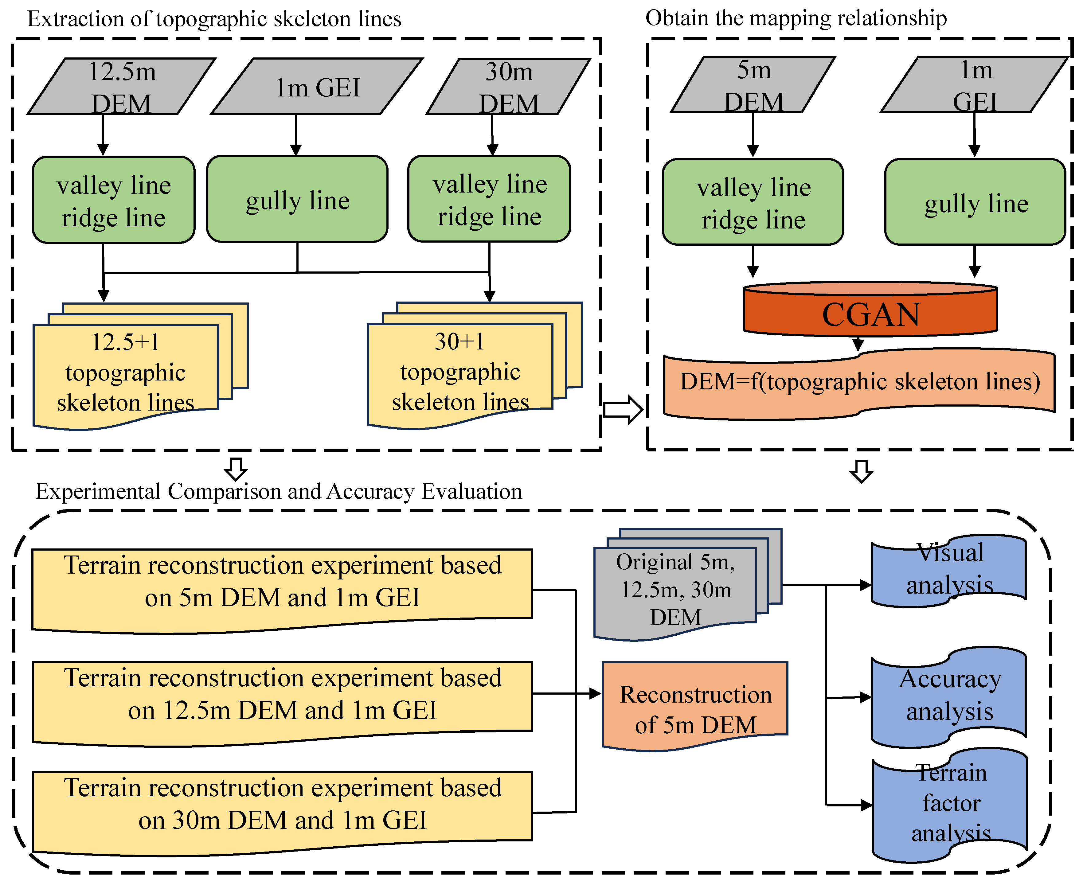
The overall workflow is shown in Figure 1. Firstly, ridge and valley lines were extracted using the original 5 m DEM, and gully lines were extracted using GEI. Moreover, ridge lines, valley lines, and gully lines were fused to obtain the mapping relationship between the DEM and the skeleton line, using CGAN. Then, ridge and valleys lines were extracted using the 12.5 m and 30 m DEMs and were separately fused with gully lines extracted from GEI. Finally, the 5 m DEM was reconstructed by merging three terrain datasets through a created mapping relationship. A visual analysis, accuracy analysis, and terrain factor analysis were carried out on the reconstructed DEM, as well as the original 5 m, 12.5 m, and 30 m DEMs.
2.2. Data Description
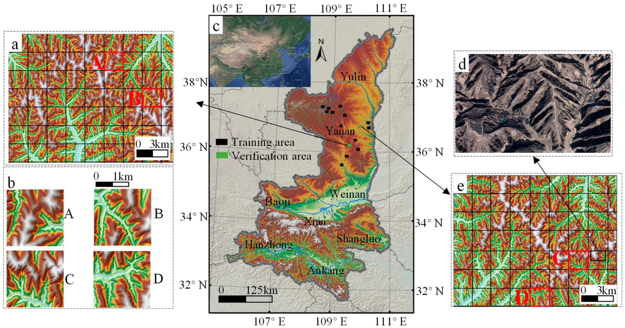
The Loess Plateau in Shaanxi Province, China (Figure 2c), was selected as the study area. The study area forms gullies and rugged landscapes due to the complex climate, loose soil, wind, and rainfall erosion, thereby complicating terrain modeling [44,45]. This selection allows the model to tackle complex terrain whilst confidently validating the outcome. Multi-scene 5 m DEMs of the Loess Plateau were selected to address the large volume of training samples needed (Figure 2c) and verified training effectiveness on the DEMs of two scenes, the Ganquan County area (Figure 2a) and the Yanchuan County area (Figure 2e), which were divided into 112 sample areas that represented the unique Hills and Gullies terrain of the Loess Plateau, respectively. Only four sample areas are displayed (Figure 2b) due to the limited size of the paper.
Three types of data were used in this study, as shown in Table 2. The high-precision 5 m resolution DEM, obtained from the National Bureau of Surveying and Mapping of China, was employed to study elevation sequences between high-precision skeleton lines and the 5 m DEM. The ALOS PALSAR RTC (Phase Array type L-band Synthetic Aperture Radar Radiometric Terrain Correction) 12.5 m DEM and ASTER V3 30 m DEM were obtained from open-source platforms, and the 1 m resolution GEI was obtained from Google Earth.
Maintaining spatial resolution, which is the critical attribute in the field of geography, is essential to complying with the stringent input requirements of the CGAN. Therefore, the training and validation data must undergo cropping. The training samples in this paper were set as squares with a side length of 256 pixels, demonstrating an actual side length of 1.28 km for each sample. Consequently, the 12.5 m DEM, 30 m DEM, and 1 m GEI data were all cropped to squares with a side length of 1.28 km. A total of 112 samples were obtained after cropping the 5 m DEM and GEI of Ganquan (Figure 2a) and Yanchuan (Figure 2e), from which four were randomly selected as display samples for this study (Samples A, B, C, and D in Figure 2b).
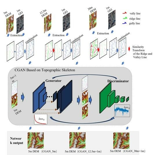
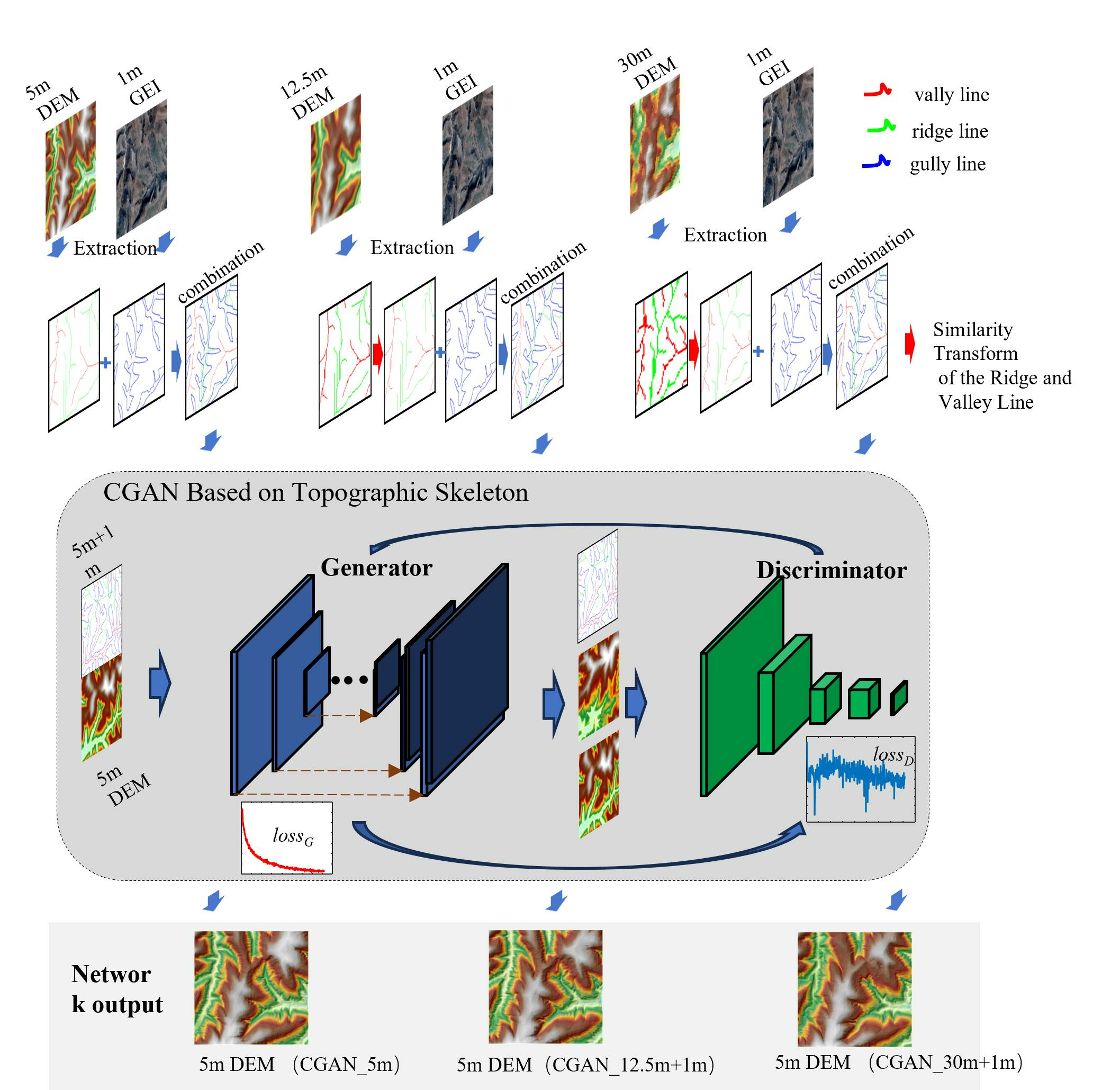
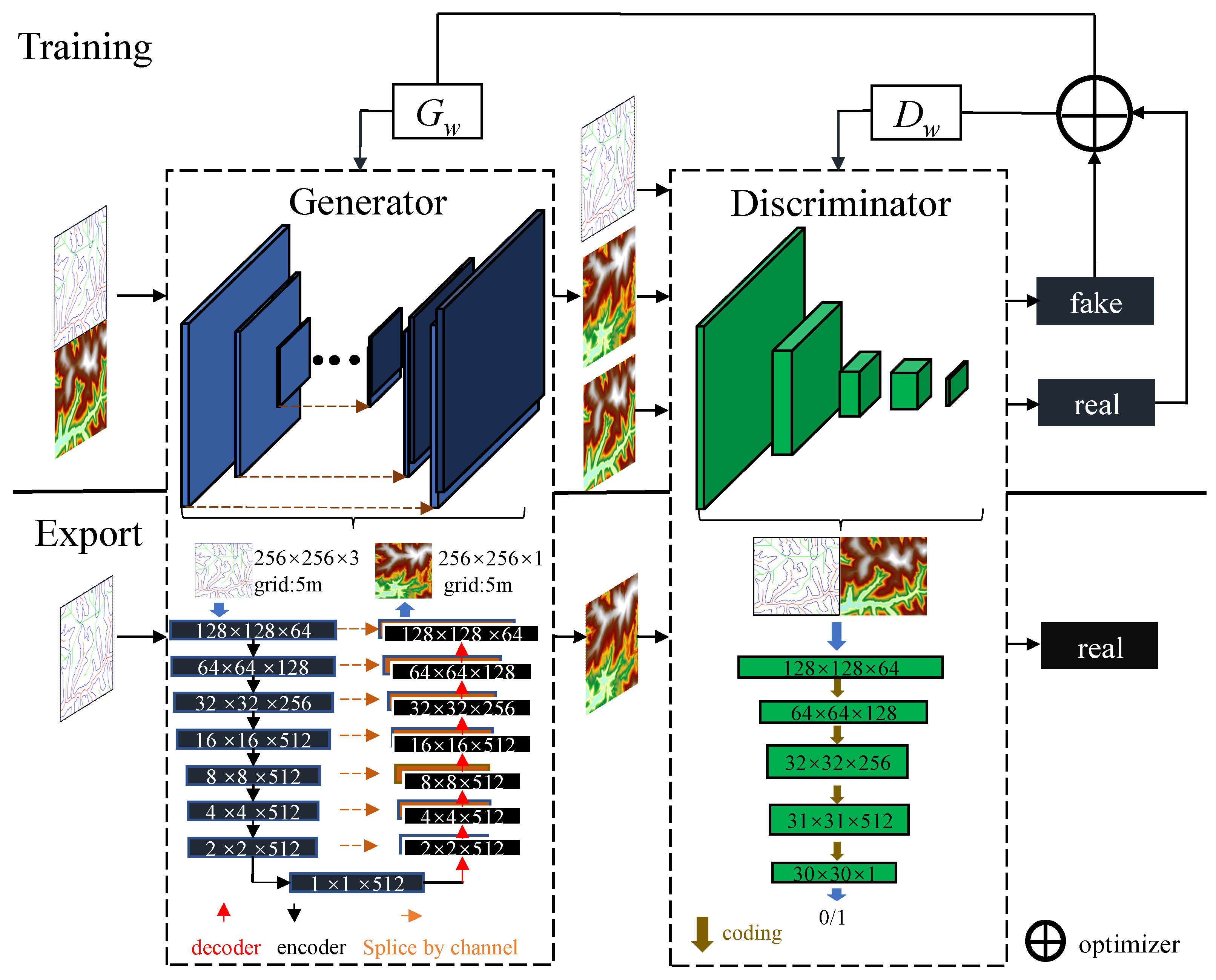
2.3. CGAN Based on Topographic Skeleton
A network model based on CGAN and pix2pix was used in this paper [29,30] (Figure 3). CGAN comprises a generator and a discriminator, with the generator creating the image and the discriminator determining the similarity between the image generated by the generator and the original image. In addition to inputting random noise, CGAN differs in that it also adds control conditions such as topographic skeletons to enhance terrain control. The terrain is continuous; thus, terrain details must be preserved during down-sampling to maintain the topographic skeleton. The generator uses the U-Net structure to input the topographic skeleton into each layer of the down-sampling process [29] and adds a skip-connection layer between the input and output matching codecs to enhance feature maps and conditions. The computer vision technique generally processes RGB images. However, the DEM is a single-band image matrix; therefore, the output must be modified to one band in the final convolution layer of the generative model. The loss function of the generator needs an error function to compare the generated DEM to the original, and the total loss function of the generator is as follows:
where is the loss value of the generator, is the number of samples, refers to the probability that the generated DEM is judged to be true by the discriminator, ε is the correction of error, is the weight of the original GAN, is the weight of the difference between the fake and real, is the original DEM, and is the fake DEM.
The discriminator operates by determining whether the input topographic skeleton resembles the original DEM. The network structure of the discriminator is illustrated in Figure 3, and this structure is comparable to that of the U-Net encoder in the generator, except for the first and last two layers. The primary layer of the discriminator’s input data is the topographic skeleton matrix alongside the corresponding original DEM after collocation. Equation (3) demonstrates that the discriminator optimization objective function is identical to the GAN loss function. The output of the loss function is then inputted into the generator to adjust the loss function, thereby facilitating the objective of using the discriminator to provide feedback to the generator.
where is the loss value of the discriminator, is the number of samples, is the probability that the generated DEM is judged to be false by the discriminator, is the correction of error, and refers to the probability that the generated DEM is judged to be true by the discriminator.
The overall loss function is the weighted sum of the generator and discriminator loss functions. This function can be represented by Formula (4).
where is the weight of the loss function of the discriminator.
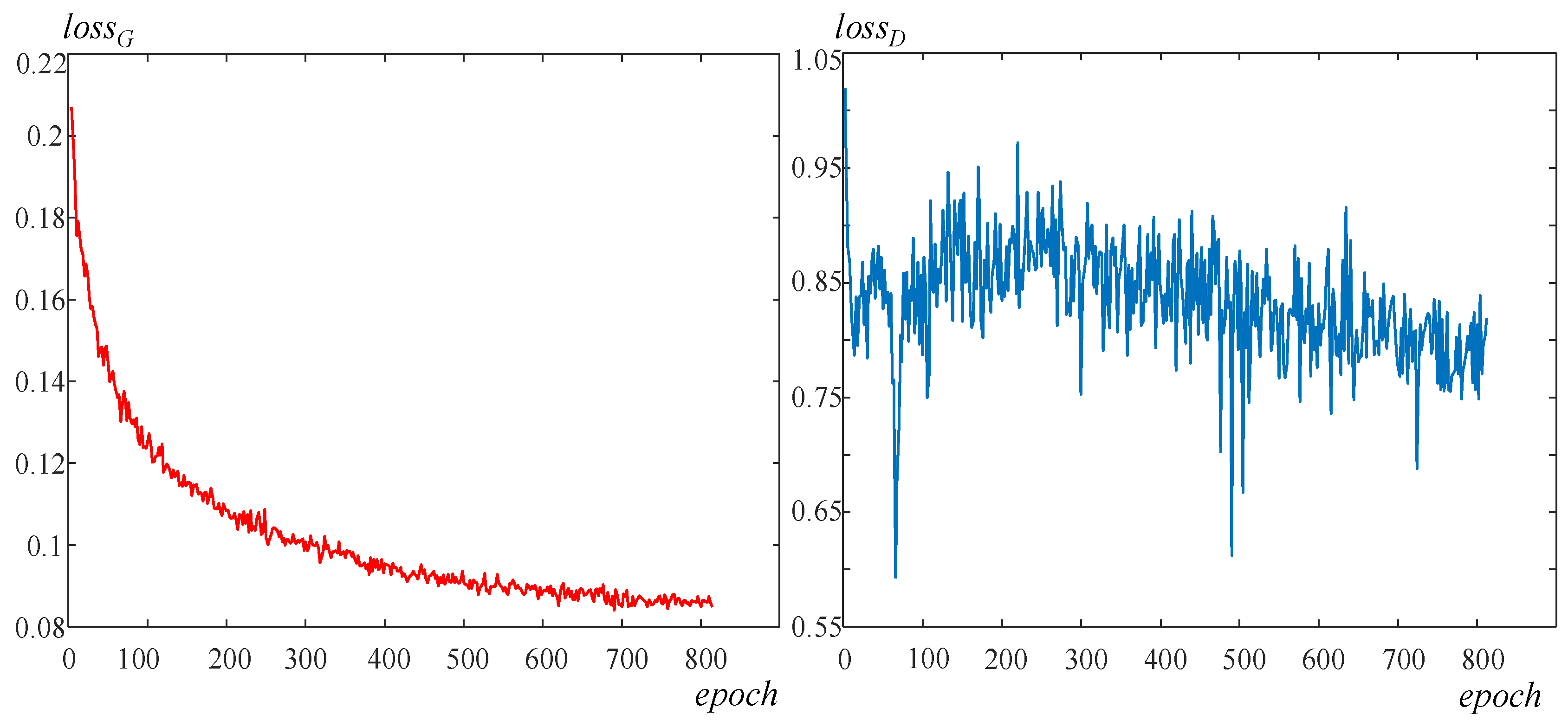
This article obtained about 2000 samples after cropping the existing 5 m DEM data of the Loess Plateau, set the batch size to 5, and used the Adam optimizer (with a learning rate of 0.002, a β1 of 0.5, and a β2 of 0.999), and the number of epochs was 600. Because DEM and the RGB images in computer vision are different, this article set the weight of the L1 loss in the generator loss function to 99. The generator’s loss function and the discriminator’s loss function curve are shown in Figure 4.
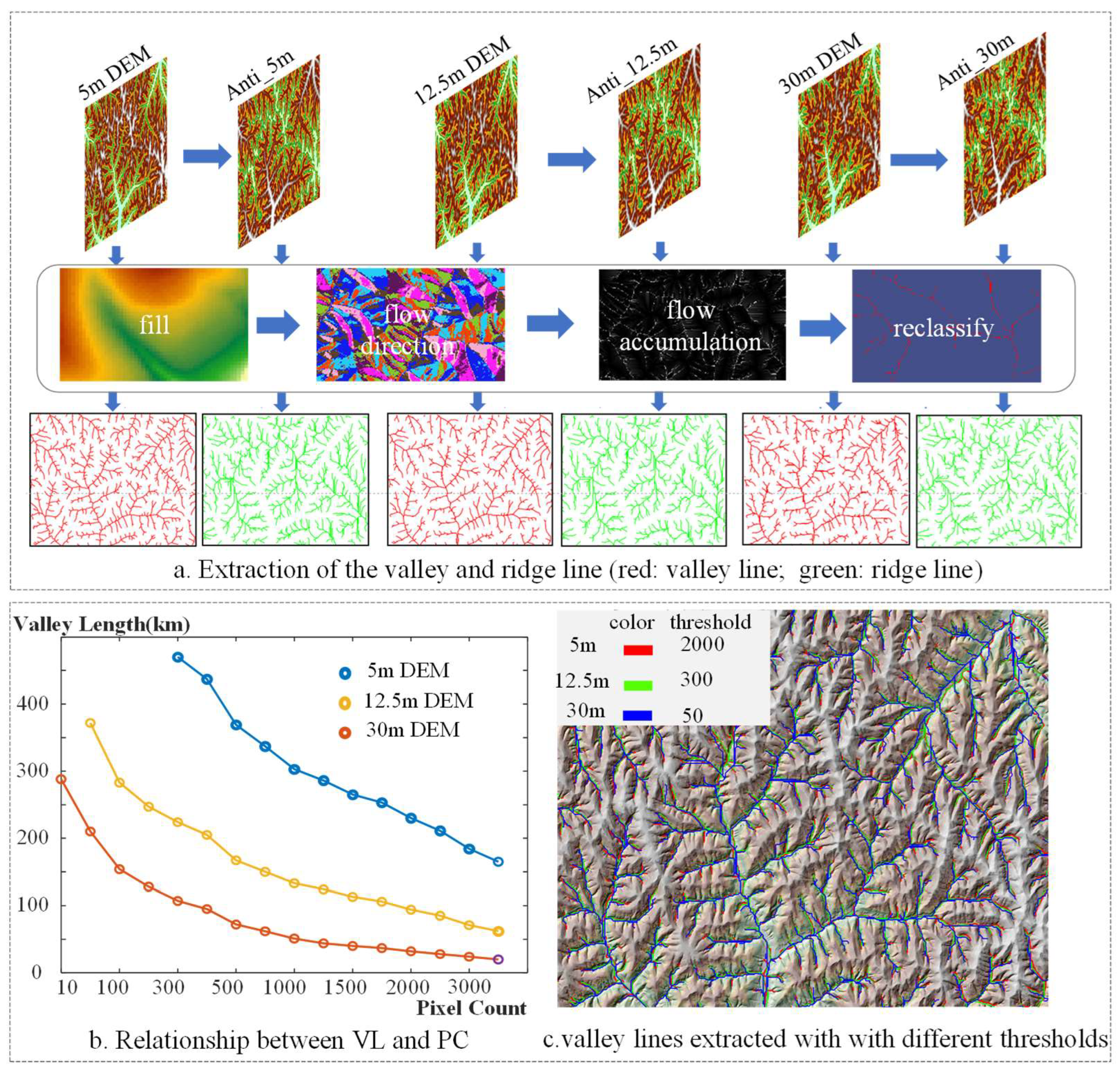
2.4. Similarity Transform of the Ridge and Valley Line
This study selected the hydrological analysis method [46] to extract ridge and valley lines (Figure 5a). The hydrological analysis method uses pixel elevation and searches for the lowest value of raster element amongst the eight surrounding neighborhoods as the outlet. The method involves puddle filling, flow direction calculation, flow accumulation calculation, and river network classification. The extraction of the ridge line is similar to the valley line of the inverse DEM. The extraction of the hydrological analysis method depends on the flow accumulation. A substantially small threshold value for extracting an excessive number of elements affects the network grading, whilst a substantially large threshold inadequately represents the details. Li et al. [30] found that the extraction of ridge and valley lines using a 5 m DEM threshold of 2000 (catchment pixels) has a superior effect on topography control in the Loess Plateau. The valleys extracted by different-resolution DEMs for the same number of catchment pixels vary significantly. From Figure 5, we see that the lengths of valley extracted from the 5 m DEM with a threshold of 2000 are close to those extracted from the 12.5 m DEM with a threshold of 300 and the 30 m DEM with a threshold of 50. Therefore, in this paper, ridge and valley lines are extracted with the 5 m DEM threshold of 2000, the 12.5 m DEM threshold of 300, and the 5 m DEM of 50. After transforming the ridge and valley lines obtained from DEMs of different resolutions to the same length, it is also necessary to convert the grid size to that of 5 m DEMs. The specific method is as follows: extract the ridge and valley lines after threshold conversion, and then resample the obtained skeleton lines to match the grid size of the training data.
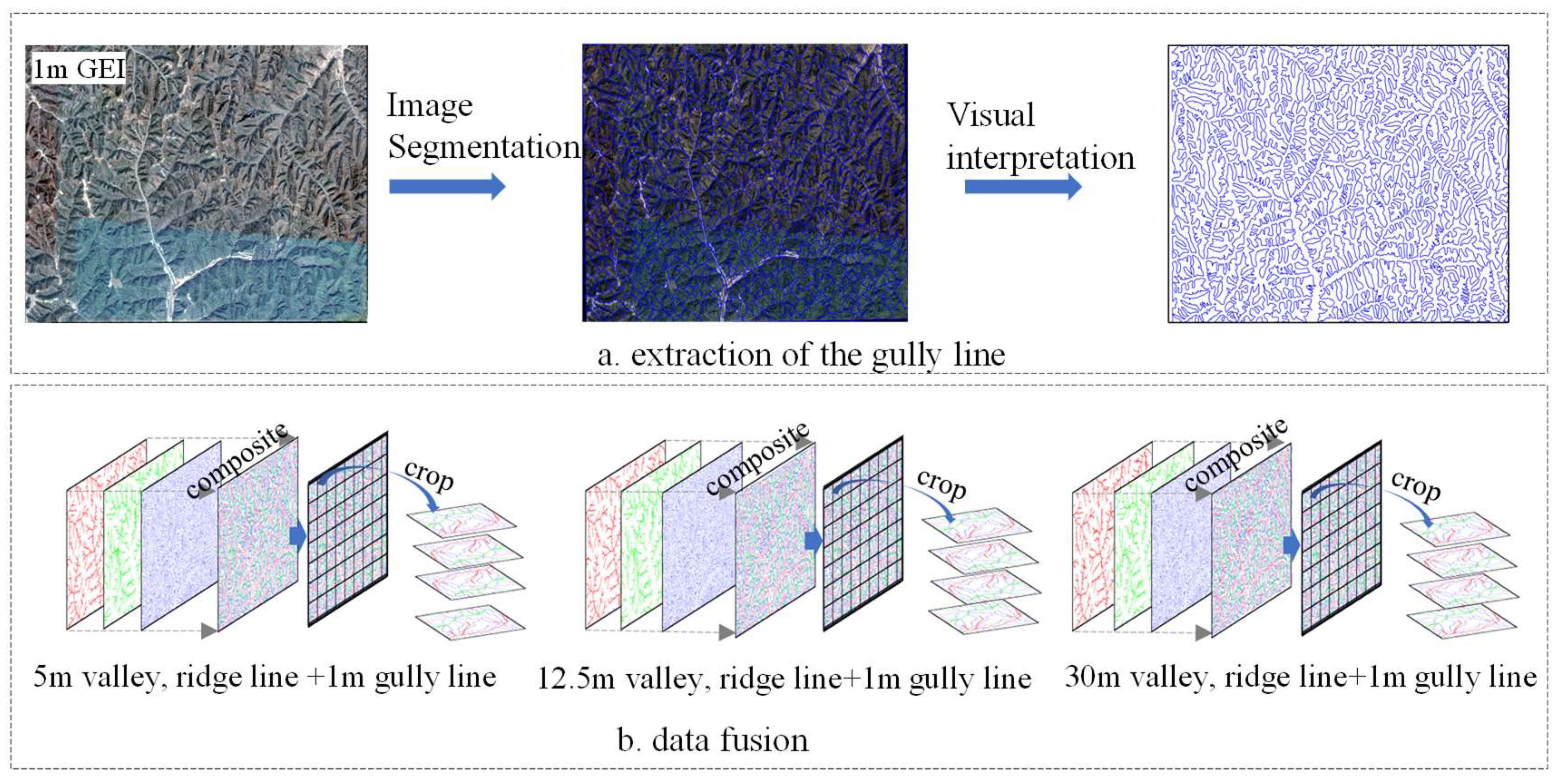
2.5. CGAN Input Data Production
The gully lines were extracted by using an object-oriented analysis method that combines remote-sensing images and the DEM [47,48] in this study (Figure 6). In this study, the software named eCognition from the Trimble company was used for multiscale segmentation; we chose a multiscale segmentation scale of 120, a shape index of 0.1, and a tightness of 0.5. The ridge and valley lines of the three-resolution DEM, as well as the gully lines from the GEI, were combined into a three-band matrix. To meet the training requirements of CGAN, the three-band matrix composed of the ridge, valley, and gully line needed to be combined with the corresponding 5 m DEM in the training dataset.
2.6. Performance Evaluation
To evaluate the effectiveness of three deep-learning methods for reconstructing 5 m DEMs from three data sources, this assessment is categorized into three aspects: (1) The first is the analysis of the vision to determine whether the reconstructed 5 m DEM was visually similar to the original 5 m DEM. (2) The correlation analysis, RMSE analysis, and mathematical indicators of elevation examine the effect of the constructed DEM and measure the disparity between the reconstructed and the original 5 m DEM. The RMSE equation is provided as Equation (5) [49]. (3) The slope and aspect extracted from the original 5 m DEM, as well as those from the original 12.5 m and 30 m DEM, are utilized as reference models in this paper to compare the slope and aspect generated by various schemes and determine the differences in slope morphology between the generated and original terrain.
where in this paper refers to the comparison DEM pixel with 5 m DEM, and is the corresponding reconstructed 5 m high-precision DEM image value.
3. Results
3.1. Visual Comparison
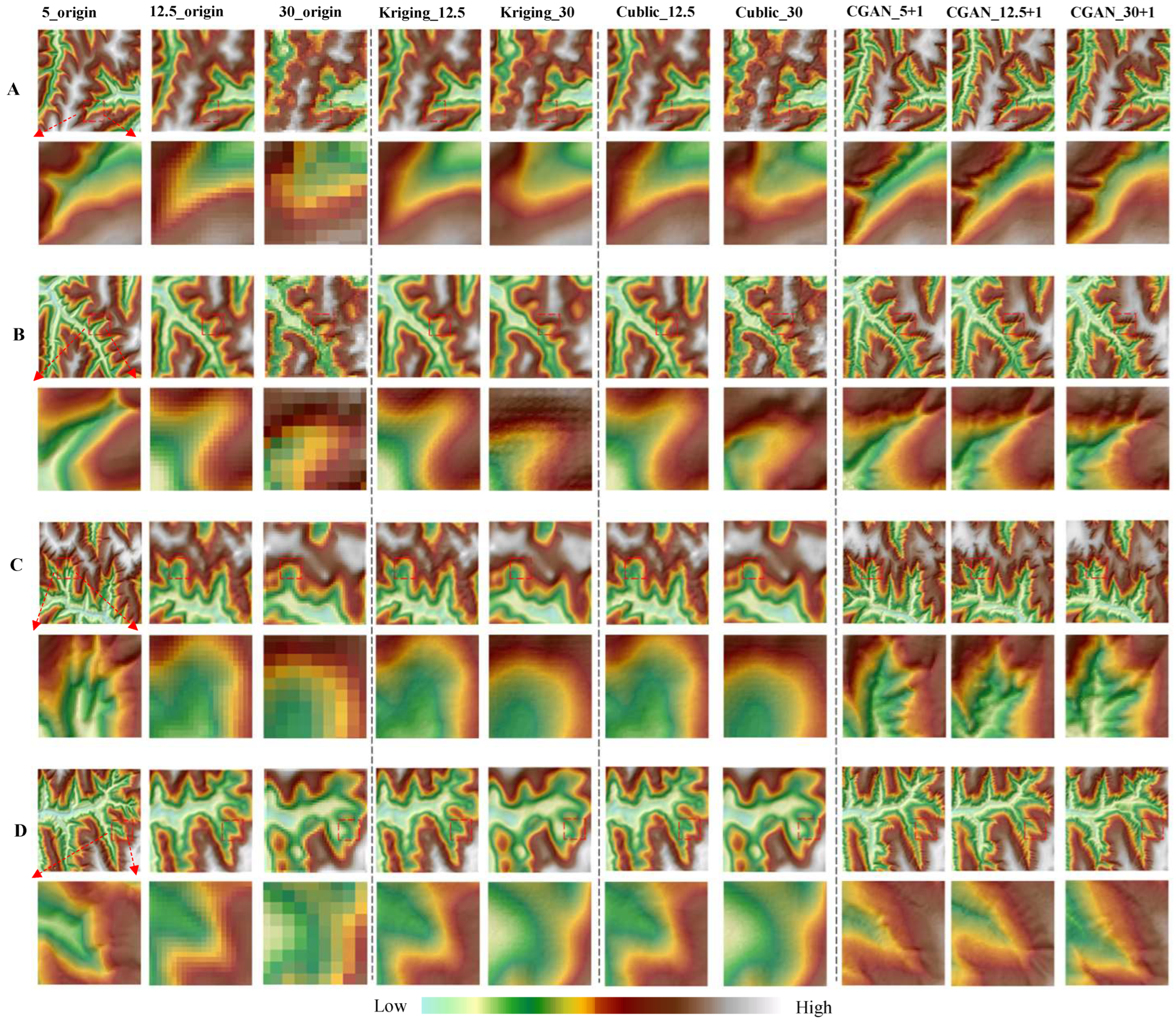
This paper proposes terrain-modeling methods and evaluates their performance against traditional interpolation methods, as shown in Figure 7. The traditional interpolation method used is ordinary Kriging and Cublic, the chosen semi-variogram model is the Spherical model, and the search radius is set to 50 in the Kriging method. Deep-learning methods generally outperform traditional interpolation methods in producing grayscale maps and hillshade with better-reconstructed contours and shapes. Traditional interpolation methods barely show any improvement when compared to the original 12.5 m and 30 m DEMs. Compared with the original DEM, the interpolation methods still lack the rich information provided by the deep-learning method to identify and add terrain information despite their improvement in smoothness and terrain detail. This limitation is attributed to the limited amount of information provided by interpolation methods during high-to-low-resolution conversion by utilizing the spatial autocorrelation law. By contrast, deep-learning methods have created an information repository through supervised learning, which allows them to obtain additional information. Therefore, the following discussion focuses solely on comparing the terrain modeling results of the deep-learning method.
Comparing the original three-resolution DEMs with the reconstructed terrain based on the deep-learning methods shows that the latter better reflects surface relief, especially in gully areas. This finding indicates that the trained model can preserve a topographic skeleton to the resultthat is comparable to the original 5 m DEM. Additionally, the reconstructed 5 m DEM captures more information and details regarding the gully slope than the original 5 m DEM due to the high-quality information and details provided by the 1 m GEI. Nevertheless, the reconstructed details do not accurately display the end of some branch gullies. This limitation is attributed to the threshold value selection of the hydrological analysis method, which fails to extract small threshold values of branch gullies, leading to a suboptimal reconstruction outcome. The comparison of the hillshade images reveals that the 5 m reconstructed DEM is smooth at the prominence of ridges, with a substantially gradual slope change. This phenomenon may be induced by the mismatch between the ridge line extracted from the 5 m DEM and the gully line extracted from the 1 m GEI. In conclusion, compared with the original three-resolution DEMs and the traditional interpolation method, the 5 m DEM reconstructed by deep-learning methods completely outperforms the original 12.5 m DEM, the 30 m DEM, and the traditional interpolation method in terms of the visual effects.
3.2. Accuracy Analysis
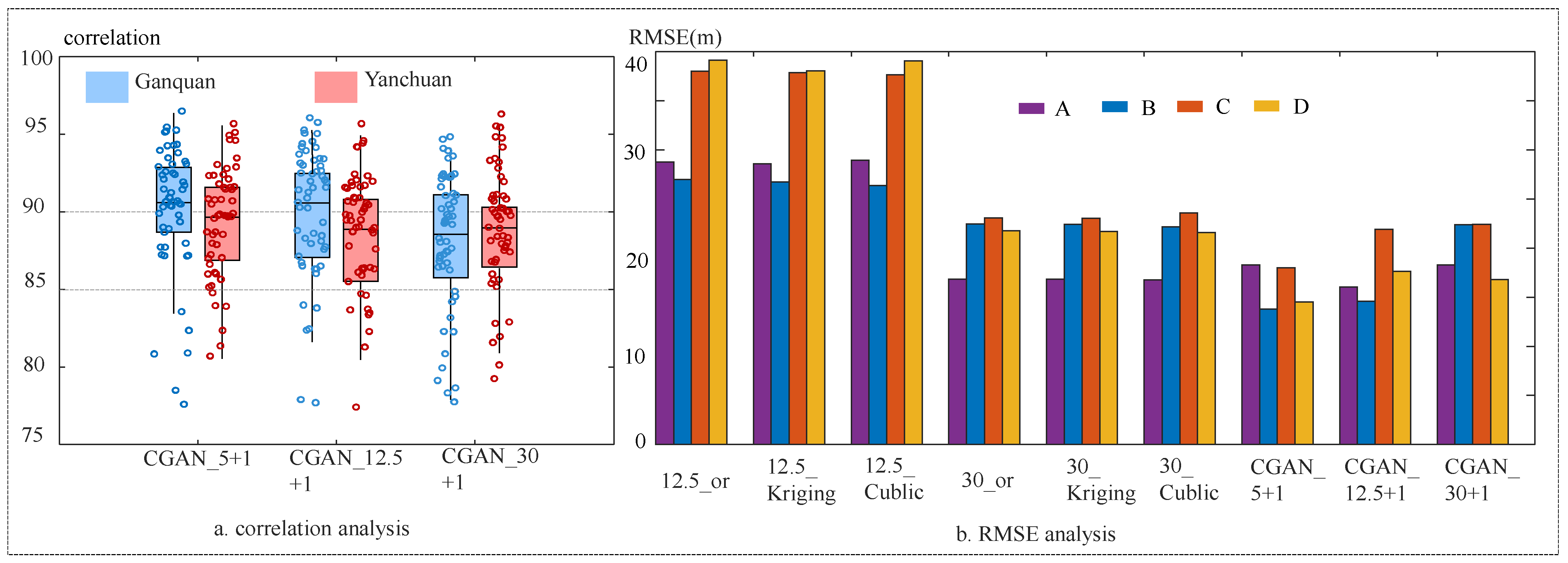
This study presented experimental designs on the correlations amongst 112 sample areas in two study fields to evaluate the efficacy of the elements extracted from three distinct data sources in reconstructing a 5 m DEM and reducing the impact of randomness. Box plots of the correlation coefficients of 112 experiment samples were illustrated to compare differences (Figure 8). The results show that the 5 m DEM combination of 1 m GEI reconstructed the best 5 m DEM, followed by the 12.5 m combination and then the 30 m combination for both research areas. Moreover, the reconstructed 5 m DEM from the three data sources in the sample areas’ analyses reveals a correlation greater than 0.85, with a median greater than 0.90, indicating the excellent reliability of the model output. Therefore, this study proves that the quality and data information in the reconstructed 12.5 m DEM and 30 m DEM data are remarkably superior; in some instances, they are equivalent to the DEM reconstructed by 5 m elements. This method can potentially reconstruct selected areas lacking high-resolution DEM by utilizing information from Google Earth Image and GDEM.
This study collected all points after vectorizing four sample areas, using the original 5 m DEM elevation values as checkpoints for the vertical elevation accuracy of seven data groups. The findings show that the ASTER 30 m DEM outperforms the ALOS 12.5 m DEM in vertical accuracy. Whilst the interpolation method has a minimal impact on vertical accuracy, deep-learning methods demonstrate different outcomes. Specifically, the proposed method in this study has a more significant impact on improving the ALOS 12.5 m DEM vertical accuracy compared to the other methods. However, the proposed method had a less significant effect on vertical accuracy for the 30 m DEM because the RMSE of vertical accuracy from the 5 m DEM reconstructed by deep learning is between 10 and 20 m compared to the original 5 m DEM. Therefore, the 5 m DEM reconstructed using other data by transferring methods does not exceed the original 5 m DEM. These findings indicate that the proposed method can enhance the quality of the ALOS 12.5 m DEM in horizontal and vertical dimensions. By contrast, this method can only improve ASTER 30 m DEM horizontal geomorphological information.
Table 3 shows the mathematical statistics of the elevation of the four sample areas by comparing the mean, maximum, minimum, and standard deviation of the raster elevation of the three data sources, the two interpolation methods, and the three deep-learning methods. It can be seen that the traditional interpolation methods have almost no change for the mathematical properties of the data, only affecting the smoothing, and the deep-learning methods have a greater improvement in the quality of the data. Among the three deep-learning methods, the effect of utilizing the 12.5 m DEM with the 1 m GEI is comparable to that of fusing the 5 m DEM with the 1 m GEI, but it is significantly better than that of fusing the 30 m DEM with the 1 m GEI. This indicates that utilizing the 12.5 m DEM with the 1 m GEI can achieve comparable results to the original DEM reconstruction.
3.3. Terrain Factors’ Analysis
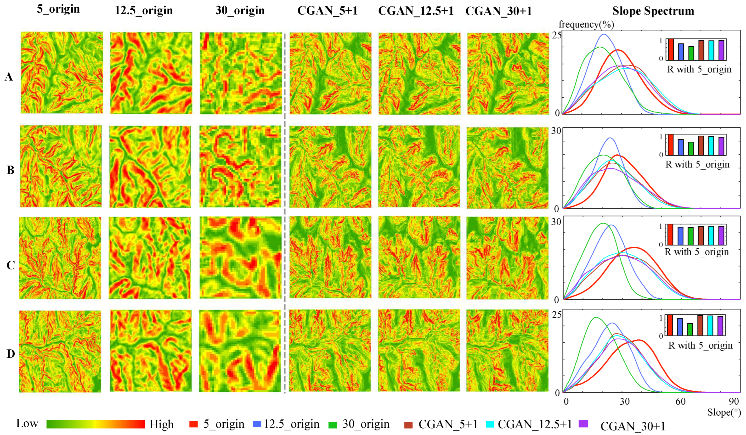
This study compared the slope maps and spectra of the reconstructed DEMs with the original 5 m DEM extracted using various methods, and the results are presented in Figure 9. The analysis results of the slope of the original 5 m DEM and the reconstructed DEM at three different resolutions revealed that all three deep-learning methods demonstrate a superior performance in reconstructing the 5 m DEM compared to the 12.5 and 30 m DEMs’ reconstruction results, as depicted in Figure 9. The 5 m DEM’s reconstruction provides a clearer and more detailed portrayal of the gully than that of the 12.5 and 30 m DEMs, particularly in terms of detail.
The comparison results of the slope profiles of different datasets indicate that the reconstructed slope trends of the 5 m DEM, which utilizes the deep-learning method, are significantly consistent (as illustrated in Figure 9), and the correlation with the slope curve of the 5 m DEM is high. All the reconstructed slopes propagate the same peak and slope configurations as the extracted slope of the original 5 m DEM, whilst also displaying higher slope reductions than the 12.5 and 30 m DEMs’ expressed slopes. In relatively complete watershed areas, the slope histogram is approximately a Gaussian distribution. Low-resolution DEMs fail to represent the small areas containing high slopes effectively due to the effects of external natural aspects, such as wind and water forces. Therefore, the slopes extracted from the 5 m DEMs obtained by the three deep-learning methods are close to those extracted from the original 5 m DEM.
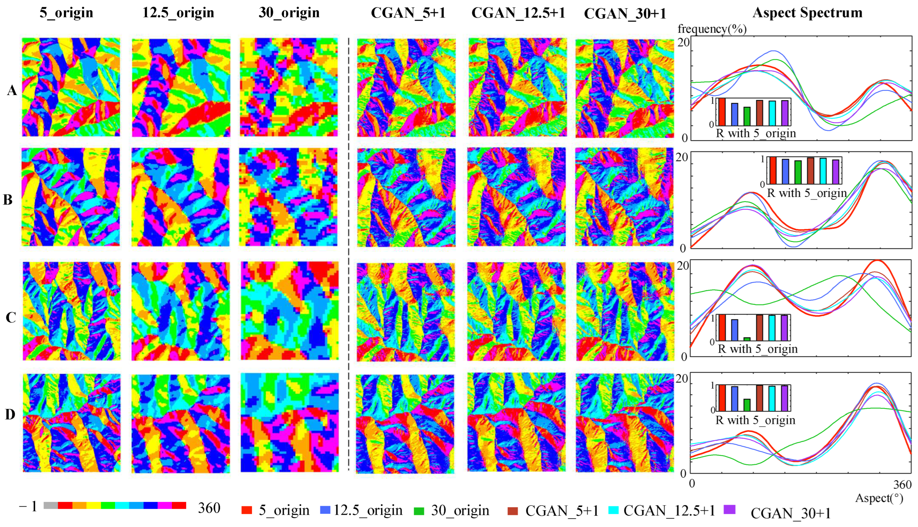
The aspect indicates the direction with the largest elevation change and helps determine the orientation of the terrain slope. Aspect information can be derived from sunlight, which is critical for plant growth and temperature. In the geographical studies, the aspect map is an image represented with element values ranging from −1 to 360. The aspect is categorized into eight directional interval values. When the aspect graphs of the three sets of original DEMs and the three sets of reconstructed DEM data were analyzed in eight directions (as shown in Figure 10), the datasets demonstrated significant differences in aspect expression, particularly those derived from the 30 m original DEM, compared to other datasets. This finding suggests that the resolution has a significant influence on the aspect. The aspect of the 5 m DEM extracted by the three deep-learning methods was closest to the original 5 m DEM, with the same trend noted in the reconstructed 5 m DEM. This finding demonstrates that this model works well for aspect expression and can effectively recover the aspect information of the original DEM.
4. Discussion
4.1. Effect of Similarity of Topographic Skeleton
4.1.1. Influence of the Topographic Skeleton Length
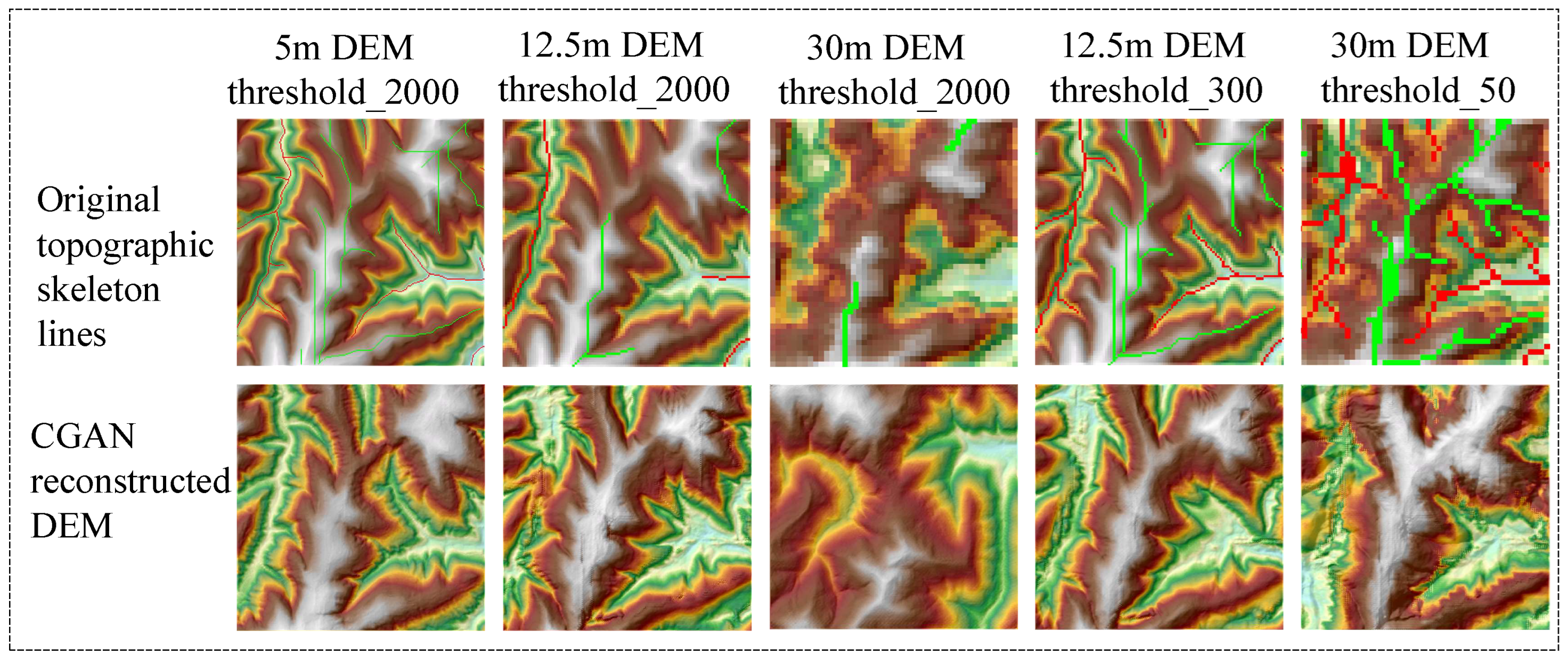
The ability to reconstruct the 5 m DEM from three different-resolution DEMs is primarily determined by the topographic skeleton, specifically the extraction of the topographic skeleton’s lines from the DEM. The gully line is used as a constant value in this experiment for reconstructing the DEM from the three data sources. Therefore, the reconstruction effect primarily depends on the ridge and valley lines. The extraction results of ridge and valley lines depend on the chosen threshold of flow accumulation. Due to different resolutions, the same threshold will cause significant differences in river network length, resulting in severe distortion when reconstructing DEMs at other resolutions (Figure 11). Therefore, a threshold transformation is needed to better enable other resolution DEMs to obtain an approximation of training 5 m DEMs. Similar input terrain skeletons guarantee similar output 5 m DEMs from the deep-learning network. From Figure 11, it can be seen that the distortion is larger when the 12.5 m and 30 m DEMs are used with a threshold of 2000. The ridge and valley lines of the 30 m DEM are missing when the threshold is too bad, resulting in a loss of control over the terrain, causing great deformation. The reconstructed 5 m DEM is less distorted compared to the original 5 m DEM after using the converted threshold obtained from Section 2.4.
4.1.2. Influence of the DEM Grid Size
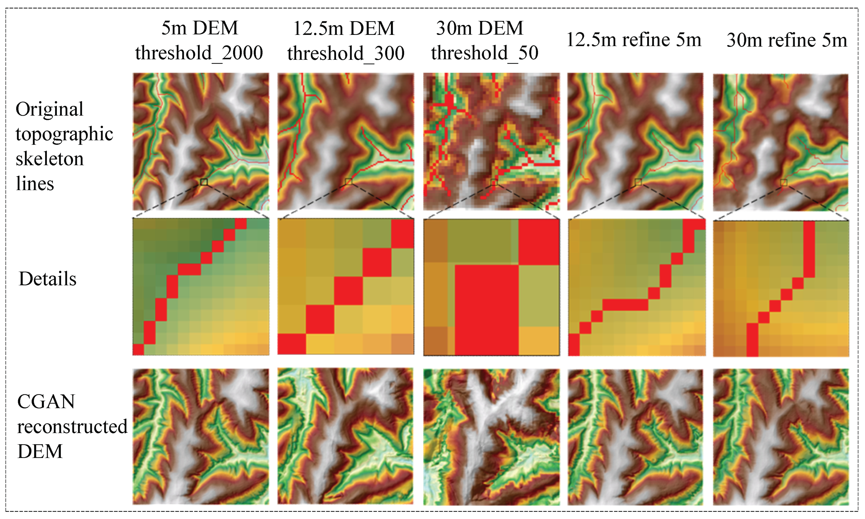
Although the ridge and valley lines at the same length constrain the generation of the terrain, it can be seen through Figure 11 that the 12.5 m and 30 m DEMs are still greatly distorted when utilizing the same length of skeleton lines as the 5 m DEM. Therefore, further work is needed, which is performed by refining the skeleton lines extracted from the 12.5 m DEM and 30 m DEM to obtain the same grid size of skeleton lines as that of the 5 m DEM. Figure 12 illustrates the terrain reconstructed by CGAN with different DEM resolutions at similar spatial locations and the same length of the river valley. When the difference in image elements between the 5 m grid and the training image element is large, the generated topography offset is high, resulting in a poor reconstruction effect. Therefore, refining the topographic skeleton lines of other resolution DEMs to the same grid size as the 5 m DEM is necessary.
4.2. Difference with the Traditional Interpolation Method
The traditional interpolation method uses mathematical rules for inferring unknown points’ values from the existing points. This method works well in the regions with flat terrain. The deep-learning method proposed in this paper is dependent on the terrain skeleton, so it is more effective in regions where the terrain skeleton is obvious (i.e., mountainous areas) but less effective in regions where the terrain skeleton is unobvious (i.e., a chain of undulating hills without obvious ridge and gully). The traditional interpolation method makes it hard to increase the additional information into the original data, while the deep-learning method has established a nonlinear fitting relationship through a large number of training data, and can add information through the established mapping relationship between the terrain skeleton and the DEM, which makes it possible to recover the terrain. This also explains the superior results of the deep-learning method. Table 4 demonstrates the difference between the deep-learning method in this paper and the interpolation method.
4.3. Application of the Void Filling of DEM
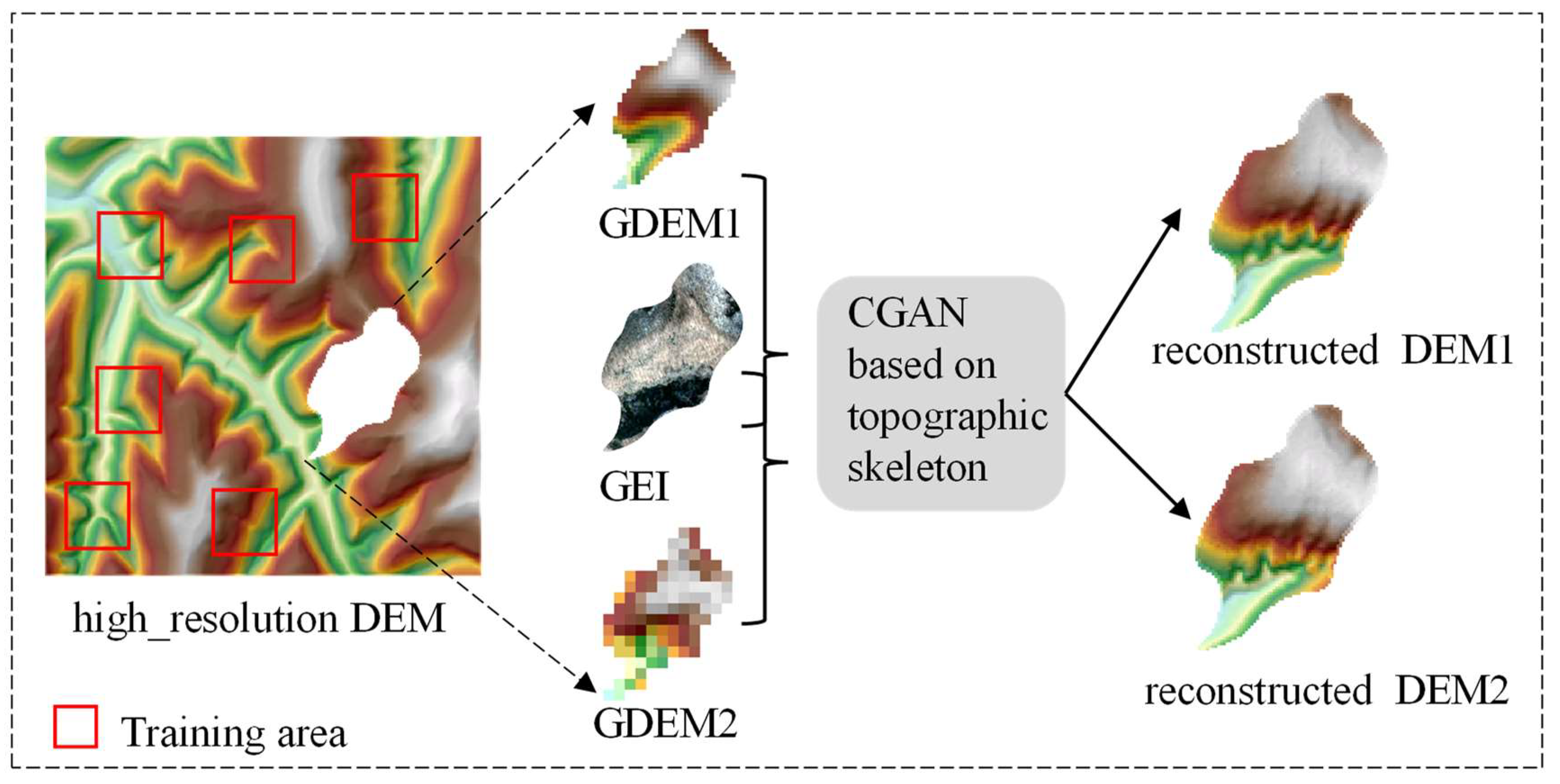
Nowadays, the mainstream acquisition techniques of DEM are mainly optical photogrammetry and radar interferometry; the former is susceptible to other factors, such as clouds, fog, etc., and the latter is of poorer quality in complex areas, such as mountainous regions, and prone to cause voids. The method proposed in this paper significantly outperforms traditional interpolation methods. Thus, this method can utilize existing data for training and extract topographic skeleton lines by GDEM to fill in voids in some high-resolution DEMs. As illustrated in Figure 13, if we have a high-resolution DEM for a certain study area but it contains missing data that need to be filled, we can utilize the existing data for training to establish the relationship between terrain skeleton lines and the DEM. Then, we can use an open-source GDEM to extract the terrain skeleton lines for the missing parts and transform the same length and grid conversion. Finally, we put the transformed terrain skeleton lines into the trained network to obtain terrain reconstruction.
5. Conclusions
This paper presents a framework for reconstructing high-precision DEM, using GEI, GDEM, and CGAN, which utilize feature-recovery details in computer vision. Topographic skeletons (valley, ridge, and gully lines) were extracted from GDEM and GEI. These elements are used as constraints to generate the DEM, using the CGAN model. Different combinations of topographic skeletons extracted from 5 m, 12.5 m, and 30 m DEMs and 1 m GEI were compared for reconstructing 5 m DEMs. The generated DEM is evaluated on the basis of its visual effect, accuracy analysis, and terrain factor analysis. The experiment’s results show that the 5 m DEMs generated with the three deep-learning methods are all similar to the original 5 m DEM (reference data), which provides a markedly increased level of terrain detail information when compared to the traditional interpolation methods. From the perspective of elevation accuracy, the correlation of reconstructed DEMs from three deep-learning methods to the original 5 m DEMs exceeds 0.9, while the vertical accuracy of the 12.5 m + 1 m combination is obviously higher than that of the 30 m DEM + 1 m GEI combination. From the perspective of topographic factors, the distribution trends of the reconstructed 5 m DEM are all close to the reference data in terms of the extracted slope and aspect. This study enhances the quality of open-source DEM and introduces innovative ideas for producing high-precision DEMs. In regions where the field survey of high-precision DEMs is difficult, open-source DEMs combined with GEI can be used in high-precision DEM reconstruction.
The difference in the effect of DEM generation from the extracted elements of different datasets primarily stems from the accuracy of the topographic skeleton extraction. Extracting topographic skeletons from open-source DEMs and GEI yielded a similar effect to the extraction of such elements from a high-precision DEM. Consequently, modeling DEMs based on open-source DEMs and GEI produces results that are similar to those of the original high-precision DEM.
Author Contributions
Conceptualization, W.D.; methodology, K.C. and J.F.; software, K.C. and M.L. (Mingyue Lu); validation, K.C. and M.L. (Mingyue Lu); writing—original draft preparation, K.C. and M.L. (Mengqi Li); writing—review and editing, K.C., W.D. and C.W.; visualization, K.C. and C.W.; supervision, C.W. and W.D.; project administration, C.W.; funding acquisition, C.W and S.L. All authors have read and agreed to the published version of the manuscript.
Funding
This work was supported by the 2023 Postgraduate Research and Innovation Program in Jiangsu Province, China (project number: KYCX23_1291); the Research and innovation team of Physical geography environment in Anhui Province, China (grant number: 2022AH010066); Research on key technologies and demonstration application of rural digital twin holography physical geography environment (project number: KJ2021ZD0130), natural science research project in Anhui Province, China, 2022–2023; physical geography environment intelligent technology industry innovation, Chuzhou “113” industry innovation team, 2022–2023; and Anhui province academic and technical leader candidate research funding project in 2018 (project number: 2018H191).
Data Availability Statement
The data that support the findings of this research are available from the author upon reasonable request.
Conflicts of Interest
The authors declare no conflict of interest.
References
- Xu, Y.; Luo, M.; Liang, B.; Chang, X.; Xiang, W.; Zhang, B. Effects of different DEM spatial interpolation methods on soil erosion simulation: A case study of a typical gully of dry-hot valley based on USPED. Prog. Geogr. 2016, 35, 870–877. [Google Scholar]
- Chen, C.; Yue, T. DEM error analysis based on conditional stochastic simulation. J. Geo-Inf. Sci. 2009, 11, 5572–5576. [Google Scholar] [CrossRef]
- Lan, J.; Yu, H.; Chen, L.; Ma, H.; Zhang, Z. Scale effect of airborne LiDAR DEM in watershed hydrological analysis and simulation. Bull. Surv. Mapp. 2020, 0, 40–46. [Google Scholar]
- Dai, W.; Qian, W.; Liu, A.; Wang, C.; Yang, X.; Hu, G.; Tang, G. Monitoring, and modeling sediment transport in space in small loess catchments using UAV-SFM photogrammetry. Catena 2022, 214, 106244. [Google Scholar] [CrossRef]
- Wang, J.; Qin, Z.; Zhao, G.; Li, B.; Gao, C. Scale Effect Analysis of Basin Topographic Features Based on Spherical Grid and DEM: Taking the Yangtze River Basin as an Example. J. Basic Sci. Eng. 2022, 30, 1109–1120. [Google Scholar]
- Dai, W.; Yang, X.; Na, J.; Li, J.; Brus, D.; Xiong, L.; Tang, G.; Huang, X. Effects of DEM resolution on the accuracy of gully maps in loess hilly areas. Catena 2019, 177, 114–125. [Google Scholar] [CrossRef]
- Mao, Y.; Song, Z.; Yue, Z.; Jia, J.; Wang, B. Application of grey scale image in terrain modeling. Fire Control Command Control 2019, 44, 160–164. [Google Scholar]
- Xu, J.; Gu, H.; Zeng, Y.; Li, X. Research on seabed terrain modeling with adaptive screen resolution. Comput. Simul. 2022, 39, 142–145. [Google Scholar]
- Dai, W.; Na, J.; Yang, X.; Cao, J. An automatic retrieval method for artificial terrace based on illumination model of DEM shading. J. Geo-Inf. Sci. 2017, 19, 754–762. [Google Scholar]
- Dai, W.; Hu, G.; Yang, X.; Yang, X.; Cheng, Y.; Xiong, L.; Josef, S.; Tang, G. Identifying ephemeral gullies from high-resolution images and DEMs using flow-directional detection. J. Mt. Sci. 2020, 17, 3024–3038. [Google Scholar] [CrossRef]
- Hayakawa, Y.; Oguchi, T.; Lin, Z. Comparison of new and existing global digital elevation models: ASTER G-DEM and SRTM-3. Geophys. Res. Lett. 2008, 35. [Google Scholar] [CrossRef]
- Perlant, F. Using Stereo Images For Digital Terrain Modeling. Surv. Geophys. 2002, 21, 201–207. [Google Scholar] [CrossRef]
- Uysal, M.; Toprak, A.; Polat, N. DEM generation with UAV Photogrammetry and accuracy analysis in Sahitler hill. Measurement 2015, 73, 539–543. [Google Scholar] [CrossRef]
- Milette, S.; Daigneault, R.; Roy, M. Refining the glacial lake coverage of the southern Laurentide ice margin using Lidar-DEM based reconstructions: The case of Lake Obedjiwan in south-central Quebec, Canada. Geomorphology 2019, 342, 78–87. [Google Scholar] [CrossRef]
- Yoo, E.; Kyriakidis, P. Area-to-point Kriging with inequality-type data. J. Geogr. Syst. 2006, 8, 357–390. [Google Scholar] [CrossRef]
- Smelik, R.; Tutenel, T.; Bidarra, R.; Benes, B. A Survey on Procedural Modelling for Virtual Worlds. Comput. Graph. Forum 2014, 33, 31–50. [Google Scholar] [CrossRef]
- Maleika, W. Inverse distance weighting method optimization in the process of digital terrain model creation based on data collected from a multibeam echosounder. Appl. Geomat. 2020, 12, 397–407. [Google Scholar] [CrossRef]
- Reichenbach, S.; Geng, F. Two-dimensional cubic convolution. IEEE Trans. Image Process. 2003, 12, 857–865. [Google Scholar] [CrossRef] [PubMed]
- Krištof, P.; Beneš, B.; Křivánek, J.; Št’ava, O. Hydraulic erosion using smoothed particle hydrodynamics. Comput. Graph. Forum 2009, 28, 219–228. [Google Scholar] [CrossRef]
- Cordonnier, G.; Cani, M.; Benes, B.; Braun, J.; Galin, E. Sculpting Mountains: Interactive terrain modeling based on subsurface geology. IEEE Trans. Vis. Comput. Graph. 2018, 24, 1756–1769. [Google Scholar] [CrossRef]
- Arakawa, K.; Krotkov, E. Fractal surface reconstruction for modeling natural terrain. In Proceedings of the IEEE Conference on Computer Vision and Pattern Recognition, New York, NY, USA, 15–17 June 1993; IEEE: Piscataway, NJ, USA, 2002. [Google Scholar]
- Arakawa, K.; Krotkov, E. Fractal modeling of natural terrain: Analysis and surface reconstruction with range data. Graph. Models Image Process. 2002, 58, 413–436. [Google Scholar] [CrossRef]
- Xiang, C.; Jia, Y. Practical algorithm of building Delaunay triangle mesh for terrain modeling. In SPIE Proceedings, Second International Conference on Image and Graphics; SPIE: Bellingham, WA, USA, 2003. [Google Scholar]
- Zhang, H.P.; Zhou, X.X.; Dai, W. A Preliminary on Applicability Analysision of Spatial Interpolation Method. Geogr. Geo-Inf. Sci. 2017, 33, 14–18+105. [Google Scholar]
- Lecun, Y.; Bengio, Y.; Hinton, G. Deep learning. Nature 2015, 521, 436–444. [Google Scholar] [CrossRef] [PubMed]
- Han, X.; Ma, X.; Li, H.; Chen, Z. A Global-Information-Constrained Deep Learning Network for Digital Elevation Model Super-Resolution. Remote Sens. 2023, 15, 305. [Google Scholar] [CrossRef]
- Jiang, Z.; Mallants, D.; Peeters, L.; Gao, L.; Camilla, S.; Gregoire, M. High-resolution paleovalley classification from airborne electromagnetic imaging and deep neural network training using digital elevation model data. Hydrol. Earth Syst. Sci. 2019, 23, 2561–2580. [Google Scholar] [CrossRef]
- Perarnau, G.; Weijer, J.; Raducanu, B.; Jose, M. Invertible Conditional GANs for image editing. arXiv 2016, arXiv:1611.06355. [Google Scholar]
- Isola, P.; Zhu, J.; Zhou, T.; Efros, A.A. Image-to-Image Translation with Conditional Adversarial Networks. In Proceedings of the IEEE Conference on Computer Vision and Pattern Recognition (CVPR), Honolulu, HI, USA, 21–26 July 2017; pp. 1125–1134. [Google Scholar]
- Li, S.; Li, K.; Xiong, L.; Tang, G. Generating terrain data for geomorphological analysis by integrating topographical features and conditional generative adversarial networks. Remote Sens. 2022, 14, 1166. [Google Scholar] [CrossRef]
- Jiang, X.; Wang, S.; Li, W.; Wang, G. DEM-cGAN framework constrained by feature lines and elevation range. J. Comput.-Aided Des. Comput. Graph. 2021, 33, 1191–1201. [Google Scholar] [CrossRef]
- Li, S.; Hu, G.; Cheng, X.; Xiong, L.; Tang, G.; Strobl, J. Integrating topographic knowledge into deep learning for the void-filling of digital elevation models. Remote Sens. Environ. 2022, 269, 112818. [Google Scholar] [CrossRef]
- Mukherjee, S.; Joshi, P.; Mukherjee, S.; Ghosh, A.; Grag, R.D.; Mukhopadhyay, A. Evaluation of vertical accuracy of open source Digital Elevation Model (DEM). Int. J. Appl. Earth Obs. Geoinf. 2012, 21, 205–217. [Google Scholar] [CrossRef]
- Kääb, A. Combination of SRTM3 and repeat ASTER data for deriving alpine glacier flow velocities in the Bhutan Himalaya. Remote Sens. Environ. 2004, 94, 463–474. [Google Scholar] [CrossRef]
- Frey, H.; Paul, F. On the suitability of the SRTM DEM and ASTER GDEM for the compilation of topographic parameters in glacier inventories. Int. J. Appl. Earth Obs. Geoinf. 2011, 18, 480–490. [Google Scholar] [CrossRef]
- Tadono, T.; Ishida, H.; Oda, F. Precise global dem generation by alos prism. ISPRS Ann. Photogramm. Remote Sens. Spat. Inf. Sci. 2014, 2, 71–76. [Google Scholar] [CrossRef]
- Guerin, É.; Digne, J.; Galin, É.; Peytavie, A.; Wolf, C.; Benes, B.; Martinez, B. Interactive example-based terrain authoring with conditional generative adversarial networks. ACM Trans. Graph. 2017, 36, 228. [Google Scholar] [CrossRef]
- Yang, X.; Tang, G.; Xiao, C.; Gao, Y.; Zhu, S. The scaling method of specific catchment area from DEMs. J. Geogr. Sci. 2011, 21, 689–704. [Google Scholar] [CrossRef]
- Li, S.; Dai, W.; Xiong, L.; Tang, G. Uncertainty of the morphological feature expression of loess erosional gully affected by DEM resolution. J. Geo-Inf. Sci. 2020, 22, 338–350. [Google Scholar]
- Jiang, L.; Gao, C.; Han, X.; Sun, Y.; Zhao, M.; Yang, C. Quantifying spatial similarities of drainage networks on multi-resolution DEMs. J. Geo-Inf. Sci. 2021, 23, 576–583. [Google Scholar]
- Zhu, H.; Tang, G.; Zhang, Y.; Yi, H.; Li, M. Thalweg in loess hill area based on DEM. Bull. Soil Water Conserv. 2003, 23, 43–45,61. [Google Scholar]
- Zhou, Y.; Yang, C.; Li, F.; Chen, R. Spatial distribution and influencing factors of Surface Nibble Degree index in the severe gully erosion region of China’s Loess Plateau. J. Geogr. Sci. 2021, 31, 1575–1597. [Google Scholar] [CrossRef]
- Chen, R.; Zhou, Y.; Wang, Z.; Li, Y.; Li, F.; Yang, F. Towards accurate mapping of loess gully by integrating google earth imagery and DEM using deep learning. Int. Soil Water Conserv. Res. 2023, in press. [CrossRef]
- Liang, W.; Bai, D.; Wang, F.; Fu, B.; Yan, J.; Wang, S.; Yang, Y.; Long, D.; Feng, M. Quantifying the impacts of climate change and ecological restoration on streamflow changes based on a Budyko hydrological model in China’s Loess Plateau. Water Resour. Res. 2015, 51, 6500–6519. [Google Scholar] [CrossRef]
- Zhang, X.; Li, S.; Wang, C.; Tan, W.; Zhao, Z.; Zhang, Y.; Yan, M.; Liu, Y.; Jiang, J.; Xiao, J.; et al. A study of sediment delivery from a small catchment in the loess plateau by the CS-137 method. Chin. Sci. Bull. 1990, 35, 37–42. [Google Scholar]
- Fairfield, J.; Leymarie, P. Drainage networks from grid digital elevation models. Water Resour. Res. 2004, 27, 709–717. [Google Scholar] [CrossRef]
- Yan, S.; Tang, G.; Li, F.; Dong, Y. An edge detection based method for extraction of loess shoulder-line from grid DEM. Geomat. Inf. Sci. Wuhan Univ. 2011, 36, 363–367. [Google Scholar]
- Liu, K.; Ding, H.; Tang, G.; Song, C.; Liu, Y.; Jiang, L.; Zhao, B.; Gao, Y.; Ma, R. Large-scale mapping of gully-affected areas: An approach integrating Google Earth images and terrain skeleton information. Geomorphology 2018, 314, 13–26. [Google Scholar] [CrossRef]
- Surveying Adjustment Discipline Group, School of Surveying and Mapping, Wuhan University. Error Theory and Basis of Measurement Adjustment; Wuhan University Press: Wuhan, China, 2014. [Google Scholar]
Figure 1.
Workflow of the study.

Figure 2.
Training area and validation area (a,c,e); paper display area (b); and physical geographic environment of validation area, Yanchuan (d).
Figure 2.
Training area and validation area (a,c,e); paper display area (b); and physical geographic environment of validation area, Yanchuan (d).

Figure 3.
CGAN is based on the topographic skeleton.

Figure 4.
Training details of the generator and the discriminator.

Figure 5.
Threshold conversion for different-resolution DEMs.

Figure 6.
Extraction of the gully line and fusion of topographic skeleton lines with different-resolution DEMs and GEI.
Figure 6.
Extraction of the gully line and fusion of topographic skeleton lines with different-resolution DEMs and GEI.

Figure 7.
Visual comparison. (Kriging_12.5 is the 12.5 m DEM interpolated to 5 m by using the Kriging method, and Kriging_30 is the 30 m DEM interpolated to 5 m; Cublic_12.5 is the 12.5 m DEM interpolated to 5 m by using the Cublic method, and Cublic_30 is the 30 m DEM interpolated to 5 m.). ((A,B): two Validation Sample Areas in Ganquan County; (C,D): two Validation Sample Areas in Yanchuan County). (The red box shows the feature area for comparison of several methods).

Figure 8.
Accuracy evaluation. (a) The correlation between the DEM generated by three deep-learning methods and the original 5 m DEM was calculated using 112 samples from two validation areas. (b) Comparison analysis of the RMSE between the original 12.5 m and 30 m DEMs, interpolated 12.5 m and 30 m DEMs into 5 m, three deep-learning methods, and the original 5 m DEM.

Figure 9.
Slope comparison. Comparison of slope and slope spectrum generated by three deep-learning methods and three data sources. R with 5_origin refers to the correlation between the slope spectrum extracted from the original 5 m DEM and other data. ((A,B): two Validation Sample Areas in Ganquan County; (C,D): two Validation Sample Areas in Yanchuan County).

Figure 10.
Aspect comparison. Comparison of aspect map and aspect spectrum generated by three deep-learning methods and three data sources. R with 5_origin refers to the correlation between the aspect spectrum extracted from the original 5 m DEM and other data. ((A,B): two Validation Sample Areas in Ganquan County; (C,D): two Validation Sample Areas in Yanchuan County).

Figure 11.
Influence of the thresholds. Original topographic skeleton lines refer to extracting valley lines from DEMs.
Figure 11.
Influence of the thresholds. Original topographic skeleton lines refer to extracting valley lines from DEMs.

Figure 12.
Influence of the grid size. Original topographic skeleton lines refer to extracting valley lines from DEMs. Details refer to the pixel-level details of the DEM. CGAN-reconstructed DEM refers to DEM reconstructed by inputting terrain skeleton into the CGAN network.
Figure 12.
Influence of the grid size. Original topographic skeleton lines refer to extracting valley lines from DEMs. Details refer to the pixel-level details of the DEM. CGAN-reconstructed DEM refers to DEM reconstructed by inputting terrain skeleton into the CGAN network.

Figure 13.
Procedure for filling the void parts of a high-resolution DEM.


Table 1.
The experiments of terrain reconstruction by CGAN are based on different topographic skeletons from different data sources.
Table 1.
The experiments of terrain reconstruction by CGAN are based on different topographic skeletons from different data sources.
| Experiment Name | Purpose of the Experiment |
|---|---|
| Terrain reconstruction experiment based on 5 m DEM + 1 m GEI | Evaluating the accuracy of the CGAN model as a control group |
| Terrain reconstruction experiment based on 12.5 m DEM + 1 m GEI | Investigating the feasibility of the topographic skeleton extracted from the 12.5 m DEM to generate a 5 m DEM |
| Terrain reconstruction experiment based on 30 m DEM + 1 m GEI | Investigating the ability of the topographic skeleton extracted from the 30 m DEM to generate a 5 m DEM |
Table 2.
Datasets used in this paper.
| Data | Time | Source |
|---|---|---|
| 5 m DEM | 2000–2010 | The National Administration of Surveying in China |
| 12.5 m ALOS DEM 1 | 2006–2011 | https://search.asf.alaska.edu/, accessed on 10 January 2008. |
| 30 m ASTER GDEM | 2000–2013 | https://lpdaac.usgs.gov/products/astgtmv003/, accessed on 12 September 2010. |
| 1 m Google Earth Image | 2006 | https://earthengine.google.com/, accessed on 6 March 2006. |
1 The data source of ALOS PALSAR RTC is SRTM GL1. Although its spatial resolution reaches 12.5 m, the vertical precision is very poor, but in this paper, we did not use the vertical precision information.
Table 3.
The statistics of elevation.
| Data | Mean | Maximum | Minimum | Standard Deviation | |
|---|---|---|---|---|---|
| A | 5_origin | 1325.92 | 1408 | 1220 | 39.43 |
| 12.5_origin | 1298.16 | 1369 | 1205 | 36.39 | |
| 30_origin | 1322.08 | 1399 | 1229 | 35.33 | |
| Kriging_12.5 | 1298.24 | 1369 | 1205 | 36.33 | |
| Kriging_30 | 1322.35 | 1397 | 1231 | 34.52 | |
| Cublic_12.5 | 1298.13 | 1369 | 1205 | 36.43 | |
| Cublic_30 | 1322.09 | 1399 | 1229 | 35.14 | |
| CGAN_5+1 | 1317.21 | 1398 | 1224 | 41.52 | |
| CGAN12.5+1 | 1322.14 | 1403 | 1225 | 41.29 | |
| CGAN30+1 | 1320.18 | 1401 | 1223 | 39.42 | |
| B | 5_origin | 1322.70 | 1421 | 1232 | 39.40 |
| 12.5_origin | 1297.29 | 1387 | 1218 | 37.26 | |
| 30_origin | 1331.76 | 1412 | 1244 | 37.18 | |
| Kriging_12.5 | 1297.17 | 1385 | 1219 | 36.89 | |
| Kriging_30 | 1331.56 | 1407 | 1249 | 35.38 | |
| Cublic_12.5 | 1297.34 | 1387 | 1218 | 37.26 | |
| Cublic_30 | 1331.66 | 1413 | 1244 | 37.07 | |
| CGAN_5+1 | 1322.43 | 1415 | 1235 | 40.77 | |
| CGAN12.5+1 | 1321.98 | 1415 | 1236 | 40.57 | |
| CGAN30+1 | 1322.39 | 1417 | 1234 | 45.89 | |
| C | 5_origin | 1119.31 | 1217 | 1005 | 51.31 |
| 12.5_origin | 1085.52 | 1187 | 985 | 46.42 | |
| 30_origin | 1119.57 | 1215 | 1010 | 50.68 | |
| Kriging_12.5 | 1085.56 | 1187 | 985 | 46.41 | |
| Kriging_30 | 1119.61 | 1216 | 1010 | 50.64 | |
| Cublic_12.5 | 1085.51 | 1187 | 985 | 46.41 | |
| Cublic_30 | 1119.64 | 1216 | 1010 | 50.64 | |
| CGAN_5+1 | 1115.23 | 1215 | 1009 | 49.80 | |
| CGAN12.5+1 | 1120.34 | 1216 | 1009 | 49.83 | |
| CGAN30+1 | 1121.22 | 1216 | 1011 | 51.12 | |
| D | 5_origin | 1093.66 | 1207 | 1003 | 46.90 |
| 12.5_origin | 1057.47 | 1177 | 979 | 42.77 | |
| 30_origin | 1085.73 | 1198 | 1008 | 42.25 | |
| Kriging_12.5 | 1057.29 | 1177 | 979 | 42.65 | |
| Kriging_30 | 1085.65 | 1198 | 1008 | 42.13 | |
| Cublic_12.5 | 1057.58 | 1177 | 979 | 42.84 | |
| Cublic_30 | 1085.55 | 1198 | 1008 | 42.07 | |
| CGAN_5+1 | 1090.75 | 1202 | 1008 | 42.89 | |
| CGAN12.5+1 | 1096.95 | 1199 | 1007 | 43.16 | |
| CGAN30+1 | 1097.45 | 1197 | 1007 | 43.48 |
Table 4.
The difference with traditional interpolation method.
| Method | Advantages | Limitations |
|---|---|---|
| Traditional interpolation method | Easy to use and works well for low-relief areas | The accuracy is relatively low in high-relief mountainous areas |
| The proposed method | Works well for areas with a distinct topographic skeleton and can increase the information contained in the training data | Methods are complex and require more priori data |
Disclaimer/Publisher’s Note: The statements, opinions and data contained in all publications are solely those of the individual author(s) and contributor(s) and not of MDPI and/or the editor(s). MDPI and/or the editor(s) disclaim responsibility for any injury to people or property resulting from any ideas, methods, instructions or products referred to in the content. |
© 2023 by the authors. Licensee MDPI, Basel, Switzerland. This article is an open access article distributed under the terms and conditions of the Creative Commons Attribution (CC BY) license (https://creativecommons.org/licenses/by/4.0/).
Share and Cite
MDPI and ACS Style
Chen, K.; Wang, C.; Lu, M.; Dai, W.; Fan, J.; Li, M.; Lei, S. Integrating Topographic Skeleton into Deep Learning for Terrain Reconstruction from GDEM and Google Earth Image. Remote Sens. 2023, 15, 4490. https://doi.org/10.3390/rs15184490
AMA Style
Chen K, Wang C, Lu M, Dai W, Fan J, Li M, Lei S. Integrating Topographic Skeleton into Deep Learning for Terrain Reconstruction from GDEM and Google Earth Image. Remote Sensing. 2023; 15(18):4490. https://doi.org/10.3390/rs15184490
Chicago/Turabian StyleChen, Kai, Chun Wang, Mingyue Lu, Wen Dai, Jiaxin Fan, Mengqi Li, and Shaohua Lei. 2023. "Integrating Topographic Skeleton into Deep Learning for Terrain Reconstruction from GDEM and Google Earth Image" Remote Sensing 15, no. 18: 4490. https://doi.org/10.3390/rs15184490
Note that from the first issue of 2016, this journal uses article numbers instead of page numbers. See further details here.