Article

Discrimination of Leaves in a Multi-Layered Mediterranean Forest through Machine Learning Algorithms

by
Cesar Alvites
1,*,
Mauro Maesano
2,
Juan Alberto Molina-Valero
3,
Bruno Lasserre
1,
Marco Marchetti
1 and
Giovanni Santopuoli
4
1
Dipartimento di Bioscienze e Territorio, Università degli Studi del Molise, Cda Fonte Lappone snc, 86090 Pesche, Italy
2
Department of Innovation in Biological, Agro-Food and Forest Systems—DIBAF, University of Tuscia, 01100 Viterbo, Italy
3
Faculty of Forestry and Wood Sciences, Czech University of Life Sciences Prague (CZU), 16 500 Prague, Czech Republic
4
Dipartimento di Agricoltura Ambiente e Alimenti, Università degli Studi del Molise, Via De Sanctis snc, 86100 Campobasso, Italy
*
Author to whom correspondence should be addressed.
Remote Sens. 2023, 15(18), 4450; https://doi.org/10.3390/rs15184450
Submission received: 19 July 2023 / Revised: 7 September 2023 / Accepted: 8 September 2023 / Published: 10 September 2023
(This article belongs to the Special Issue New Advancements in the Field of Forest Remote Sensing)

Abstract

:
Terrestrial laser scanning (TLS) technology characterizes standing trees with millimetric precision. An important step to accurately quantify tree volume and above-ground biomass using TLS point clouds is the discrimination between timber and leaf components. This study evaluates the performance of machine learning (ML)-derived models aimed at discriminating timber and leaf TLS point clouds, focusing on eight Mediterranean tree species datasets. The results show the best accuracies for random forests, gradient boosting machine, stacked ensemble model, and deep learning models with an average F1 score equal to 0.92. The top-performing ML-derived models showed well-balanced average precision and recall rates, ranging from 0.86 to 0.91 and 0.92 to 0.96 for precision and recall, respectively. Our findings show that Italian maple, European beech, hazel, and small-leaf lime tree species have more accurate F1 scores, with the best average F1 score of 0.96. The factors influencing the timber–leaf discrimination include phenotypic factors, such as bark surface (i.e., roughness and smoothness), technical issues (i.e., noise points and misclassification of points), and secondary factors (i.e., bark defects, lianas, and microhabitats). The top-performing ML-derived models report a time computation ranging from 8 to 37 s for processing 2 million points. Future studies are encouraged to calibrate, configure, and validate the potential of top-performing ML-derived models on other tree species and at the plot level.

1. Introduction

Forests globally provide numerous goods and services that support human well-being [1]. The accurate assessment of forest resources is mandatory to implement sustainable forest management (SFM) and other forest management strategies to improve forest resilience, promote biodiversity conservation, and fight climate change. National forest inventories are among the most important sources of information on forest resources, allowing the assessment of forest health and productivity at different scales. Integrating remote sensing technology with traditional inventory techniques allows for the accurate and periodic monitoring of forest ecosystems at unprecedented resolution scales [2,3]. Light-detection and ranging (LiDAR) devices, such as a terrestrial laser scanner (TLS), have become powerful tools for monitoring forest structure, providing an accurate and rapid representation of a tree’s structure at a millimetric resolution [4,5,6,7,8]. The very high-resolution point clouds acquired using TLS devices allow for the characterization of vertical and horizontal forest structures at the individual tree level [9,10] in pure and multi-layered mixed-tree-species forests [11]. Tree size, straight, and shape were explored for standing trees using TLS point clouds, allowing for the quantification and classification of timber assortments [12] with a bias towards the discrimination of leaves, branches, and trunks of standing trees.
Discriminating the leaves from standing trees (e.g., tree stems and branches) improves the characterization of the tree’s structure [13,14], the quantification of stem volume, above-ground biomass (AGB), and the carbon stored in the AGB. Indeed, the most accurate tree measurements can be obtained in TLS point clouds labeled as timber through several tools, such as quantitative structure modeling (QSM), SimpleTree [15], CompuTree (https://computree.onf.fr/; accessed on 9 September 2023), 3D FOREST (https://www.3dforest.eu/; accessed on 9 September 2023), OPALS (orientation and processing of airborne laser-scanning data; https://opals.geo.tuwien.ac.at/; accessed on 9 September 2023), the python tool (i.e., TreeTool) [16], and R packages (e.g., lidR, FORTLS, ITSME) [13,17,18].
Recent approaches that discriminate the leaves from timber TLS point clouds through a binary-class approach can be divided into machine learning (ML) algorithms and computer vision (CV) approaches [13,19,20]. The construction of ML-derived models depends on various factors, such as the choice of algorithm, quality of the dataset, calibration of models (i.e., combination of hyperparameters and number of predictors), and setting of specific parameters. For instance, supervised ML algorithms, such as random forests (RFs), Gaussian mixture models (GMMs), and support vector machine (SVM), require labeled datasets and the specification of an optimal combination of hyperparameters to develop top-performing models aimed at discriminating timber–leaf point clouds [13,14,21]. In contrast, an unsupervised ML algorithm requires unlabeled datasets and the setting of specific parameters to detect hidden timber and leaf clusters in TLS point clouds. For example, to search for timber and leaf points, top-performing DBSCAN (density-based spatial clustering of applications with noise models)-derived models required setting two parameters: the radius between the centroid and the cluster boundary and the minimum number of points inside the created cluster [22]. The neglected configuration of ML algorithms during the construction of models can result in overfitting, underfitting estimations, erroneous predictions, unstable performances, and the necessity for a significant amount of computing work [23]. Moreover, some open source tools that discriminate timber and leaf points, such as LEWOS [24] and TLSLeAF [25], are available.
Additional specific factors affecting the construction of ML-derived models are point quality, point processing, and the forest stand structure [26,27,28,29]. Particularly, (1) the laser beam dimension plays a crucial role in accurately describing leaves or small branches, directly impacting the accuracy of discrimination; (2) the distance between the TLS instrument and the tree increases and the point quality worsens as the beam dimensions increase; (3) there is an increase in point spacing in the intermediate and overstory layers due to the greater distance between objects and the TLS instrument (i.e., the farther the object is, the lower the probability to receive laser beams), presenting challenges for discriminating tall trees; and (4) dense forests with an understory can hinder the penetration of laser beams, while forests with a scarce mount of trees are expected to facilitate an accurate reconstruction of the trees in the forests [26,27,28,29]. However, these limitations can be overcome by adhering to worldwide standard TLS point cloud acquisition protocols [13,14,29]. Another limitation in many studies is the demand for advanced coding skills and high-performance PCs, rather than just the choice of an ML algorithm and input data quality (Table 1). Furthermore, although several studies achieved good timber–leaf findings, most of them were conducted in relatively simple conditions, such as deciduous or evergreen plantations or temperate forests, often involving only a few species and focusing on trees that were not tall [22,30,31,32].
To our knowledge, achieving successful millimetric tree reconstructions with TLS may be influenced by the forest stand structure, including the tree diameter and tree density in the understory and overstory vegetation layers [7,13]. Accordingly, the accuracy tends to be lower in forests characterized by a dense tree cover and multiple layers. Therefore, there is a need for TLS studies conducted in multi-layered and mixed-tree-species Mediterranean forests, mainly focusing on benchmarking ML algorithms for point classifications, emphasizing high performance, efficiency, and speed. This research becomes even more important when point clouds are collected in mixed-layered and multi-layered forests. Furthermore, this contributes to the research by accurately separating timber from leaf components, providing useful information for implementing SFM strategies and biodiversity conservation efforts by improving forest monitoring with TLS devices and aligning this with the new forest strategies to mitigate climate change.
This study aims to assess the performance of several ML-derived models for the timber–leaf discrimination task, focusing on eight distinct Mediterranean tree species. By exploring the dataset suitability and approach effectiveness, this paper addresses the following questions: what is the optimal ML approach for the binary-class classification for each Mediterranean tree species? Which dataset—individual or combined—is better suited for binary-class classification? Is the binary-class approach more suitable for distinguishing timber from leaf points than multi-class classifications? What key factors hinder the accurate binary-class classification of top-performing models, and how do these characteristics impact discrimination outcomes?

2. Materials and Methods
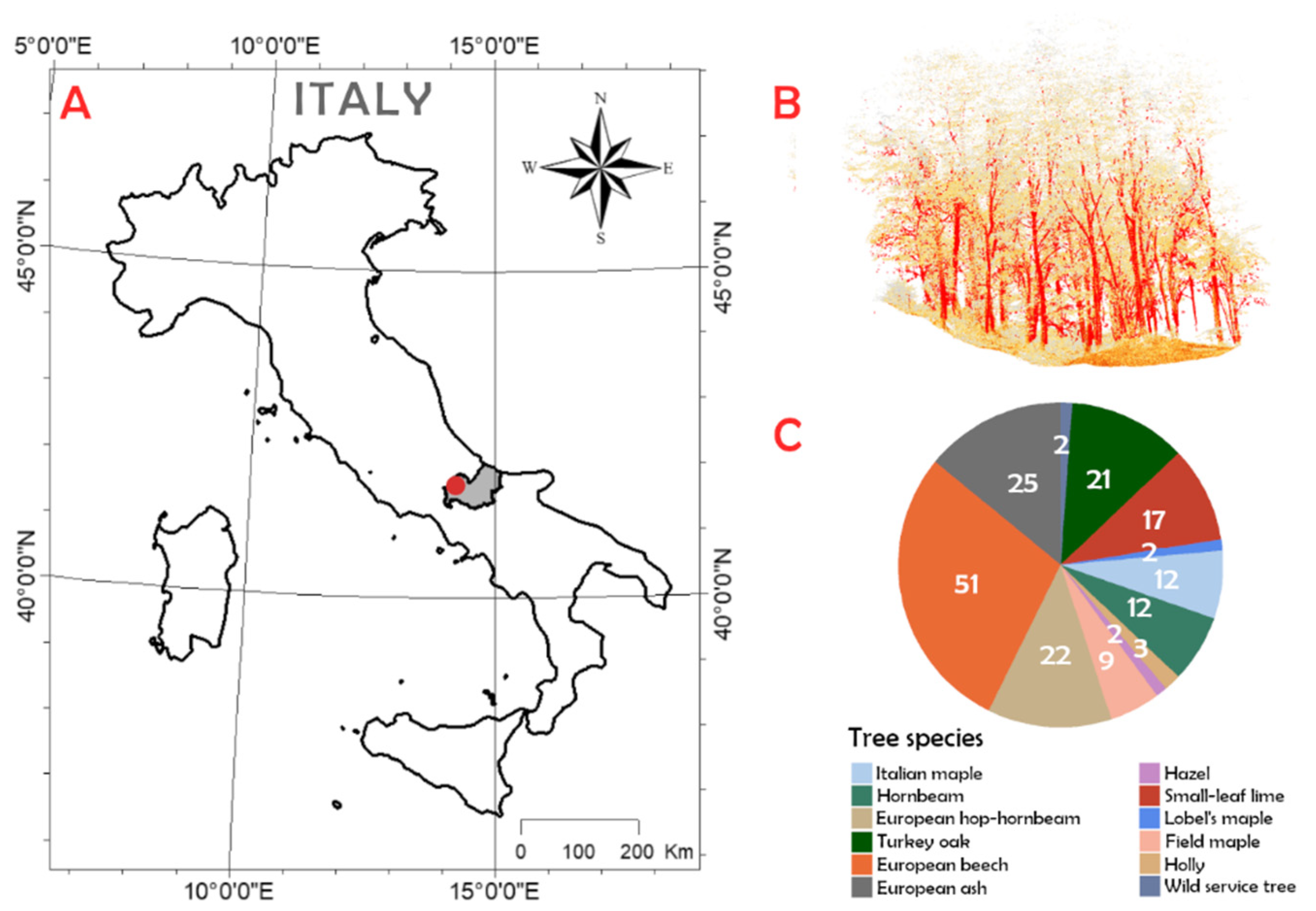
2.1. Study Area

The study area, a Mediterranean forest known for its high structural heterogeneity and rich tree species diversity, was located in the Molise Region in southern Italy (41°44′.7″N, 14°11′59.11″E) within the Bosco Pennataro (Figure 1). Covering approximately 280 ha, Bosco Pennataro belongs to the oak–hornbeam forest category and is characterized by a mesophytic deciduous forest type [36]. Bosco Pennataro is part of the Natura 2000 network and is a core area within the Collemeluccio-Montedimezzo Alto Molise Man and Biosphere (MaB) reserve. The most abundant tree species are Turkey oak (Quercus cerris L.) (40%), European beech (Fagus sylvatica L.) (21%), and Italian maple (Acer opalus Mill. subsp. obtusatum) (9.6%) [37]. Over the last 50 years, the forestry activities in this area mainly focused on conservation efforts, i.e., preventing fire events and pest attacks. Accordingly, this management type favors the conversion from even-aged to uneven-aged forest structures.

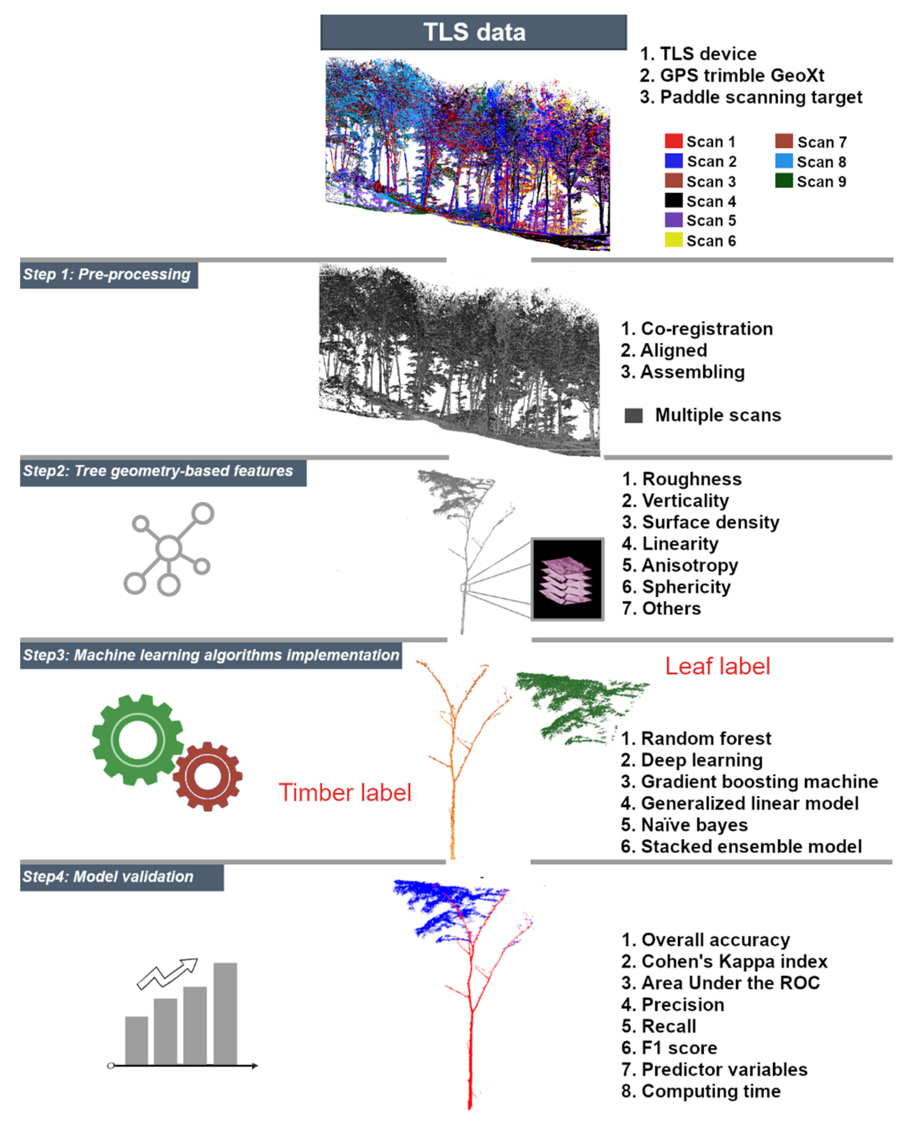
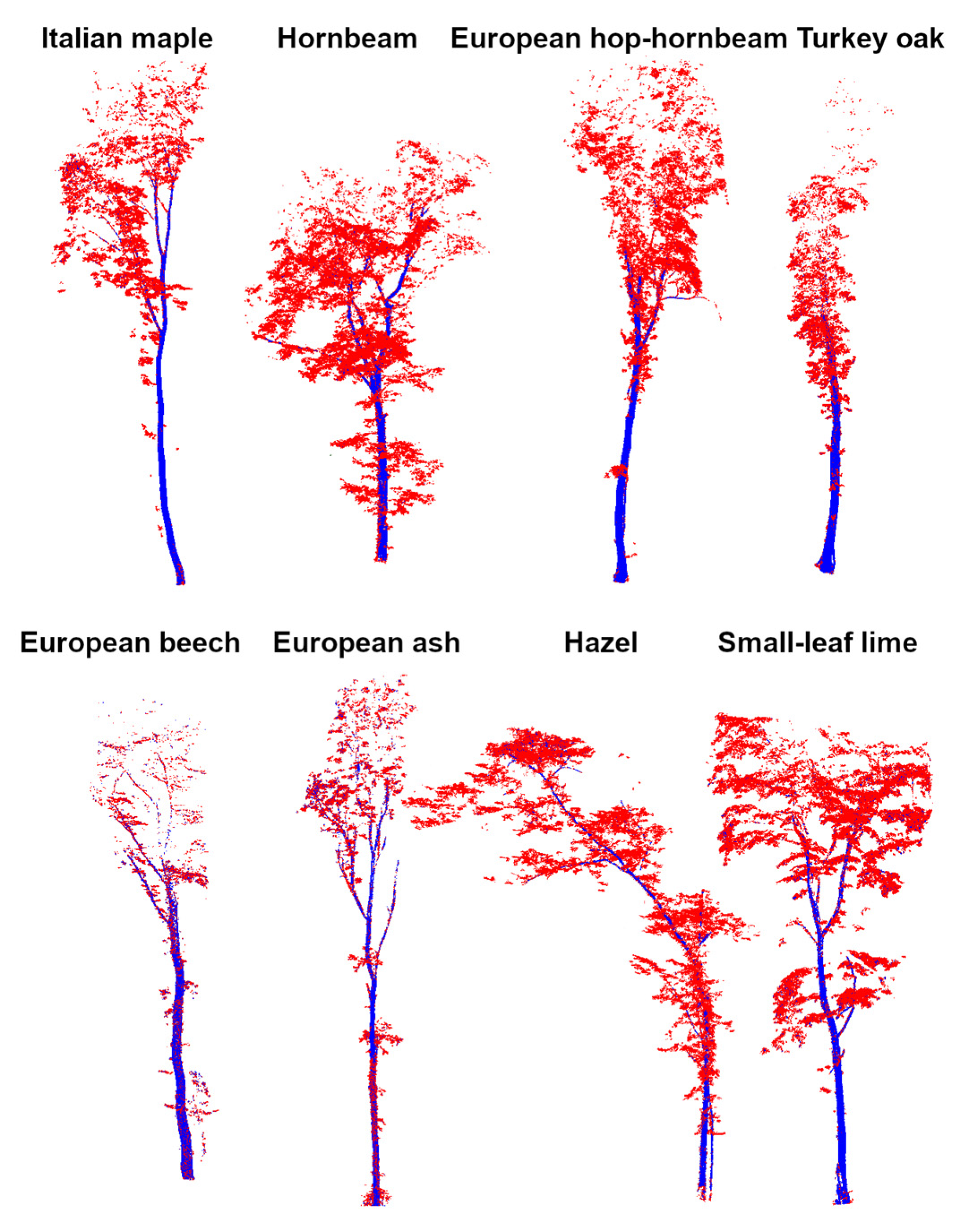
2.2. Data Collection

Ground Truth and TLS Data

The forest survey was conducted in 2016, consisting of five square plots of 529 m2 (23 × 23 m). For each tree, the following attributes were measured or estimated: tree species identification, tree vitality, tree height (TH), diameter at breast height (DBH ≥ 2.5 cm), crown projection area, crown length, vitality, and geographical position through Field-Map technology (https://www.fieldmap.cz/; accessed on 9 September 2023) [37]. More in-depth information about the sampling design implemented in the forests was explained in a previous study [38].
The TLS point clouds were acquired by Leica Scan Station P30/40 (https://leica-geosystems.com/it-it/; accessed on 9 September 2023) in July 2018. The Leica P30/40 device can record a maximum of 1 million points per second up to 270 m away, with an overall accuracy equal to ±2 mm (360° and 290° of horizontal and vertical field-of-view values, respectively) [12]. Multiple scans were recorded within each square plot to accurately describe the tree structure. On average, nine scans were acquired for each of the five square plots with point density values ranging from 36.6 to 92.2 thousand per m−2 and point spacings ranging from 3.19 to 5.22 mm [12]. The point clouds reconstructed a total of 178 standing trees with 12 tree species, and the arrangement of such scans was based on the principle of overlapping among scans (overlapping scans >30%) and the edaphic conditions explained in a previous study [12].

2.3. Data Analysis

The workflow implemented to discriminate timber from leaves in the TLS point clouds was conducted in four steps (Figure 2).

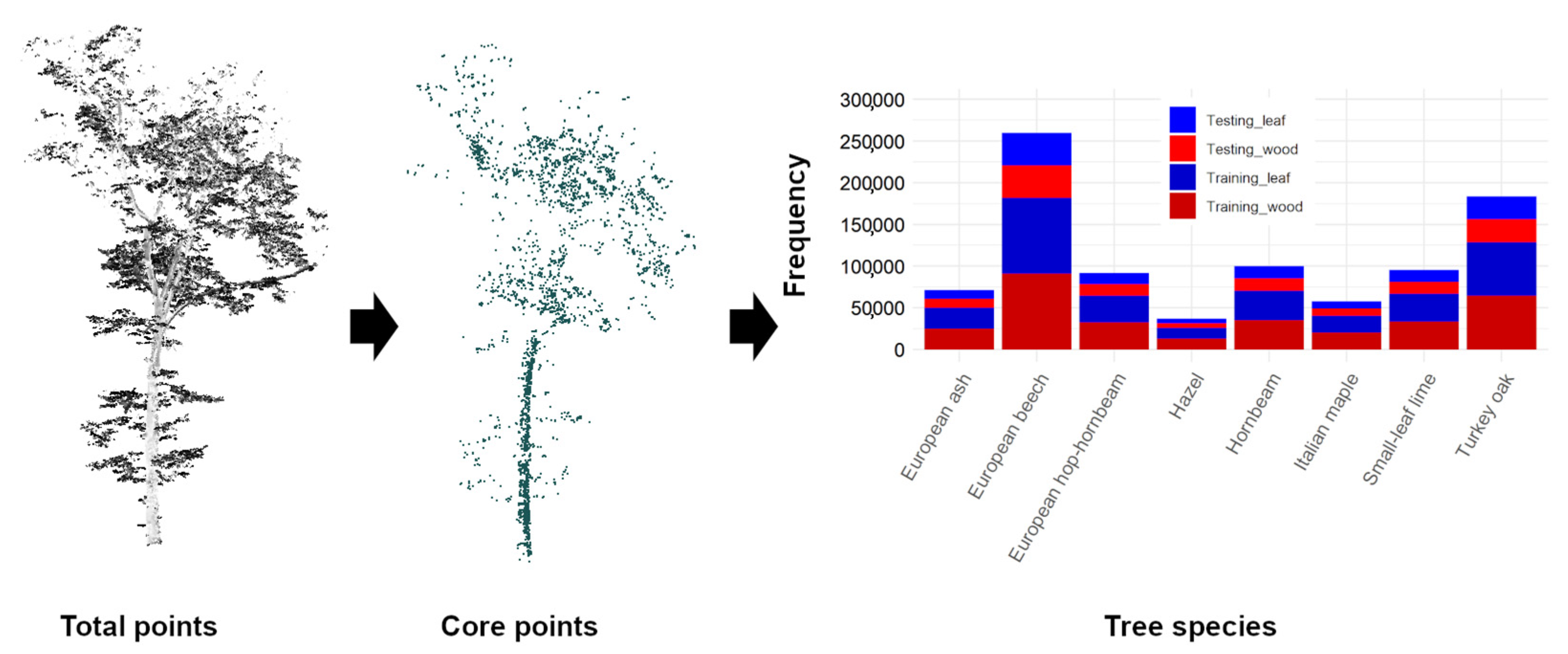
2.3.1. TLS Point Cloud Pre-Processing

When pre-processing, the multiple scans acquired by the TLS device were processed using Leica Cyclone 360 3DR V.1.7.1000 software (https://leica-geosystems.com/; accessed on 9 September 2023) and the OPALS modular program (https://opals.geo.tuwien.ac.at/; accessed on 9 September 2023), which were additionally backed by GPS Trimble GeoXt reference points [12]. In particular, the positions of paddle scanning targets within each square plot were recorded using GPS Trimble GeoXt. Subsequently, these GPS positions were used for co-registering and aligning the multiple scans using Leica Geosystems software. Finally, the co-registered and aligned multiple scans for each square plot were aligned again and assembled using the OPALS OpalsICP tool (https://opals.geo.tuwien.ac.at/html/stable/ModuleICP.html; accessed on 9 September 2023).
This step allowed us to accurately collect multiple scans, resulting in five co-registered and assembled point clouds. A total of 23 point clouds, corresponding to 8 tree species, were manually cut from the 5 point clouds using the ‘segment’ tool embedded in CloudCompare software (http://www.danielgm.net/cc/; accessed on 9 September 2023). The following eight frequent tree species were identified in the study area: Italian maple (hereafter IM), hornbeam (Carpinus betulus L.; hereafter HO), European hop-hornbeam (Ostrya carpinifolia Scop.; hereafter EHH), Turkey oak (hereafter TO), European beech (hereafter EB), European ash (Fraxinus excelsior L.; hereafter EA), hazel (Corylus avellana L.; hereafter HA), and small-leaf lime (Tilia cordata Mill.; hereafter SLL). A total of 3 point clouds were selected and segmented for each of the 8 tree species (except for HA) resulting in 23 point clouds. Subsequently, these 23 point clouds were organized into 8 separate point clouds (1 for each tree species). This step allowed us to arrange the point clouds for further investigation.

2.3.2. Tree Geometry-Based Features

In this step, the previously arranged eight point clouds were utilized as the input data for generating geometry-based features using CloudCompare software (https://www.danielgm.net/cc/; accessed on 9 September 2023). In particular, each of the eight clouds was imported into the CloudCompare software. Then, a manual classification was performed to label each point as either leaf or timber with assigned labels of 1 and 2, respectively. The same CloudCompare software was employed for the manual classification process. A subset comprising 10% of the total points (hereafter, core points) for each point cloud was randomly selected using the ‘segment’ tool in CloudCompare. Specifically, each of the 8 core points was divided equally into leaf (5%) and wood (5%) components (Appendix A, Figure A1). Subsequently, 22 different geometry-based features (hereafter, predictors) were calculated for all 8 core points, including anisotropy, eigenvalues (1st, 2nd, and 3rd), eigenentropy, sum of eigenvalues, Gaussian curvature, linearity, mean curvature, normal change rate, number of neighbors, 1st-order moment, omnivariance, principal component analyses 1 and 2, planarity, roughness, surface density, sphericity, surface variation, volume density, and verticality [12]. The method for calculating predictors involves constructing a neighborhood graph (using the k-nearest neighbor approach), extracting the features, predicting contour scores, and selecting the optimal contour, enabling the accurate characterization and detection of contours within unstructured 3D point clouds [39]. Finally, the eight core points matched with their corresponding predictors were organized into three datasets: (1) the first dataset included eight individual tree species datasets; (2) the second dataset included the combined eight datasets (hereafter, combined tree species) labeled as timber–leaf classes; and (3) the third dataset included the combined tree species dataset based on both tree species and timber–leaf class. The number of observations used for the combined tree species datasets was determined by averaging the number of observations for eight individual tree species datasets. Each dataset incorporated Cartesian coordinates (XYZ), class labels (timber, leaf, and tree species), and the mentioned predictors.

2.3.3. ML Algorithm Implementation

To assess the accuracy of the timber and leaf discrimination from point clouds, six ML algorithms, RF, naive Bayes (NB), gradient boosting machine (GBM), deep learning (DL), generalized linear model (GLM), and stacked ensemble model (EN; Table 2), were used. These ML algorithms were chosen due to their ease of use, computational efficiency, and well-established performance for the binary-class and multi-class classifications involving the discrimination of leaf (class 1) and wood (class 2) [14,27,40,41].
In this study, 60 ML-derived models were developed using 3 different datasets, as reported in Section 2.3.2. The first dataset yielded forty-eight ML-derived models after eight tree species were analyzed by six ML algorithms: RF, DL, GBM, GLM, NB, and EN. The second dataset yielded six ML-derived models after the six ML algorithms analyzed a combined tree species dataset labeled as timber and leaf classes. The third dataset yielded six ML-derived models after the combined tree species dataset labeled considering the tree species and timber and leaf classes was analyzed by the six ML algorithms. The binary and multi-class classifications used the first and second, and third datasets, respectively.
The procedural framework for the binary-class and multi-class classification approaches was structured as four main steps:
  • Importing the dataset: the three datasets were imported into the R environment (version 4.3.0) using the ‘lidR’ and ‘dplyr’ R packages [52,53].
  • Dataset partitioning: the point clouds were divided into non-overlapping training (70%) and testing (30%) sets. Each set of data was equally partitioned into leaf and wood components (Appendix A, Figure A1).
  • Model optimization: the training dataset was processed to efficiently determine the optimal combination of hyperparameters using fewer predictors [23]. The hyperparameter tuning procedure used a 10-fold cross-validation framework, while selecting predictors was conducted through a variable importance assessment. Both of these steps were executed using the ‘h2o.grid’ and ‘h2o.varimp’ functions within the ‘h2o’ package ‘h2o’ [54], ‘caret’ [55], ‘naivebayes’ [56], and ‘foreach’ [57]. Optimal hyperparameters were derived from the best model reporting the highest ‘logloss’ values (from 0% to 100%; the binary-class classification logloss equation was 1) and the ‘h2o.getGrid’ function. The logloss algorithm quantifies the cross-entropy loss of models, comparing their observed and predicted results [58].
L o g l o s s = 1 N i = 1 N w i y i ln p i + 1 y i ln 1 p i
where N is the total number of observations of the dataset, W is the user-defined weight per observation (default is 1), p is the probability of the positive class, and y is the observed true class. This research used six hyperparameters to optimize RF and DL models, while four were used for GBM and two for NB (Table 3). The ‘ntrees’ and ‘mtries’ settings for RF allowed us to control the number of decision trees and features considered for each split. Tuning the ‘ntree’ setting for GBM helped balance the learning capacity and prevent overfitting. Adjusting the activation and hidden settings in DL enhanced the model learning capacity to explore the classification patterns. The Laplace smoothing setting in NB addressed the issue of zero probability in the naive Bayes machine learning algorithm [41,51,59].
4.
Model evaluation: the top-performing models were validated through various evaluation criteria, such as statistical metrics, computation time, and predictor count. A detailed explanation of the validation approach is specified in the subsequent step (Section 2.3.4).
A distinct model optimization approach was applied to the GLM and EN models. GLM: collinearity in the GLM models was addressed by removing predictors with VIF scores exceeding 5 [60]. The best models for GLM were built using non-collinear predictors based on the AIC (Akaike information criterion) threshold in the base R environment (version 4.3.0). The selected GLM method was the negative binomial model, chosen for its superior performance in binary classifications. In contrast, for the multi-class classification, the approach applied was multinomial logistic regression embedded in the ‘nnet’ R package [61]. EN models were optimized using the ‘h2o.stackedEnsemble’ function, combining top-performing models from various algorithms.
The efficient utilization of ‘foreach’ and ‘h2o,’ coupled with high-performance computing (HPC; (https://cran.r-project.org/web/views/HighPerformanceComputing.html; accessed on 9 September 2023), played a pivotal role in enhancing the efficiency and accuracy of the model training process. Ultimately, a file containing the best 60 models—48 using individual and 12 using 6 combined tree-species datasets—was generated in the R format, to be employed in subsequent analysis phases.

2.3.4. Model Validation

The performance of the model’s classification was assessed using eight evaluation criteria [14], overall accuracy (OA), precision, recall, F1 score, Cohen’s Kappa coefficient (Kappa), area under the ROC curve (AUC), number of predictors, and computing time for model optimizations and best model implementations [27,62,63,64].
To calculate the OA (Equation (3)), precision (Equation (4)), recall (Equation (5)), F1 score (Equation (6)), Kappa (Equation (7)), and AUC measurements, a confusion matrix was created comparing predicted with observed testing data. Here, correctly classified leaf points were considered true positives (TPs), correctly classified wood points were true negatives (TNs), wood points incorrectly classified as leaves were considered false positives (FPs), and leaf points incorrectly classified as wood were considered false negatives (FNs). The confusion matrix was created using the ‘confusionMatrix’ function from the ‘caret’ package [55]. The AUC value was calculated using the ‘h2o.auc’ function available in the h2o R package [65]. These functions were assembled in R scripts and executed iteratively with the ‘tidyr’ [66] and ‘foreach’ packages [57].
N = T P + F P + T N + F N
OA = T P + T N N
Precision = T P T P F P
Recall = T P T P F N
F 1 score = 2 Precision Recall Precision + Recall
Cohen’s Kappa coefficient (Kappa) evaluates the level of agreement beyond chance and the extent of expected disagreements. P 0 represents the percentage agreement indicating the proportion of cases where raters concur (Equation (8)) and P e represents chance agreement, which reflects the agreement anticipated by random chance (Equation (9)). The output Kappa ranges from 0 to 1, with 1 indicating a complete agreement between values and higher values reflecting a better classification accuracy [64,67].
Kappa = P 0 P e 1 P e
P 0 = T P + T N N
P e = T P + F P × T P + F N + T N + F N × T N + F P N × N
The area under the ROC curve (AUC) evaluates how well a model can discriminate between true-positive and false-positive values. The optimal AUC value ranges between 0.5 and 1, where values ≤ 0.5 indicate a poor classifier.
The number of predictors used in top-performing ML-derived models was quantified to understand the models’ structures. Moreover, the most recurrent top-five predictors used by the models were investigated to understand the role of predictors in the binary-class discrimination of points across eight tree species. Furthermore, to better understand the role of predictors in top-performing ML-derived models, all top-five predictors were grouped into three groups based on bark characteristics: (a) rough corresponded to trees with rough bark traits, including TO and EA; (b) smooth included EB, HA, and HO; and c) slightly rough corresponded to trees with slightly rough bark traits, including EHH, IM, and SLL. This classification was realized based on the extensive online catalogue of Italian tree species available at https://www.actaplantarum.org/ (accessed on 30 August 2023).
To assess the practicality of the binary-class classification, we quantified the time required to optimize and implement the optimal model. Additionally, to determine the time required for classifying an unfamiliar dataset using top-performing models, a point cloud containing 2 million points was processed. The ‘system.time’ function embedded in base R version 4.3.0 was used to quantify the time for each processing step.

3. Results

Binary-class and multi-class classifications were performed at individual and combined tree-species levels, for which ten datasets (eight for individual and two for combined tree species) were processed. A high variability of point density and spacing values was observed among the tree species (Table 4), with IM reporting the lowest values (point density: 5486 pts m−2 and point spacing: 1.36 mm) and EB showing the highest values (point density: 29,175 pts m−2 and point spacing: 0.77 mm). The core point density of the combined tree species was lower than that used for the three individual tree species: HO, TO, and EB.

3.1. Hyperparameters Selected for Best Model Results

Our findings highlight the importance of the ‘ntrees’ and ‘mtries’ parameters in models that classify individual tree species datasets (ntrees = 100–500, mtries = 5–6). Notably, these parameter values are higher than those required for combined tree-species datasets (ntrees = 50; Table 5). A similar impact of the ‘ntrees’ setting was observed in GBM-derived models. In contrast, the ‘max_depth’ value for individual tree species was two-times greater than that required for the combined tree-species dataset. In addition, the main difference between the selected hyperparameters for DL within both combined datasets (binary-class and multi-class classifications, respectively) was the choice of learning models: ‘rectifier’ for multi-class and ‘maxout’ for binary-class classifications.

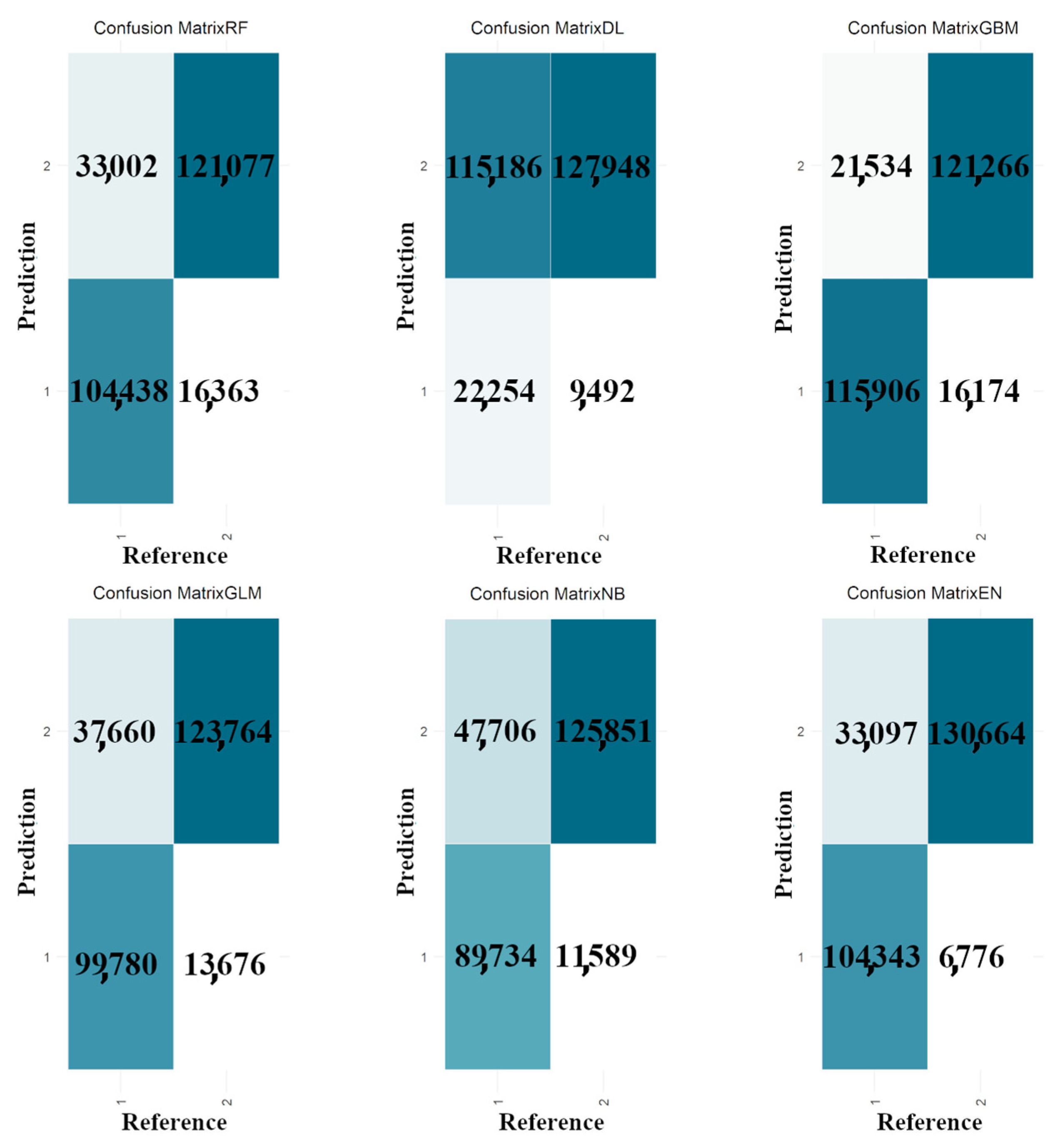
3.2. Binary-Class Classification Results for Individual Tree Species

The binary-class classification results reveal a consistent performance across all six algorithms, with average F1 scores (ranging from 0.91 to 0.92) and OA (ranging from 0.85 to 0.90) rates highlighting notable similarities across various individual tree species (Table 6). Such an outcome was supported by the well-balanced average precision and recall rates, ranging from 0.86 to 0.91 and 0.92 to 0.96 for precision and recall scores, respectively.
The RF-, GBM-, EN-, and DL-derived models achieved the highest average F1 score of 0.92 in absolute terms, corresponding to an overall accuracy of 0.90. Regarding the relative performance, RF-derived models successfully discriminated the components for 6 tree species, GBM-derived models for 5, EN-derived models for 4, and DL-derived models for 2 (Table 6 and Figure 3). In contrast, NB- and GLM-derived models achieved slightly lower accuracy than the previously mentioned algorithms, ranging between 0.90 (OA = 0.87) and 0.91 (OA = 0.88) for the F1 scores.
According to their AUC values, all top-performing ML-derived models revealed accurate discrimination scores, with the EN-derived models providing the best accuracy of up to 0.99 for HA. Additionally, there was a substantial agreement between the observed and predicted data, as supported by average Kappa values across the ML-derived models, ranging from 0.67 to 0.76.
Our finding reveals a contrasting pattern of responses among the different tree species. For instance, four of the eight tree species studied (IM, EB, HA, and SLL) showed an average F1 score rate higher than 0.94 and an average overall accuracy higher than 0.90 (Table 6 and Figure 3). On the other hand, the discrimination of timber–leaf points for HO, EHH, TO, and EA showed typical F1 score rates ranging between 0.86 and 0.90, corresponding to an average overall accuracy spanning from 0.83 to 0.88.

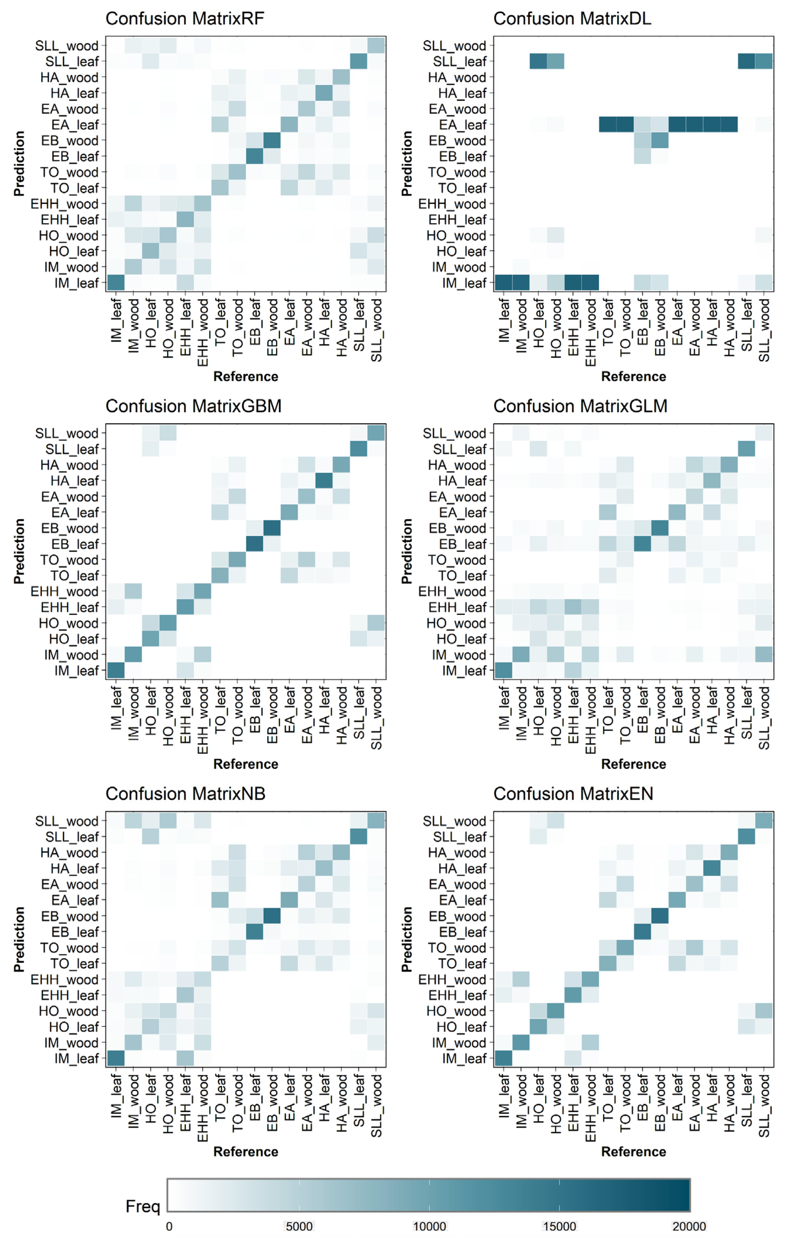
3.3. Binary-Class and Multi-Class Classification Results for Combined Tree Species Datasets

The results reveal contrasting differences between the multi-class and binary-class classifications (Table 7). Although the multi-class classification outperformed the binary-class classification in terms of F1 scores (0.89 vs. 0.81) and precision (0.94 vs. 0.74), respectively, the binary-class classification proved to be superior in terms of OA (0.78 vs. 0.49) and Kappa values (0.56 vs. 0.46), respectively.
The confusion matrices confirmed better performance for GBM- and EN-derived models (Figure 4). The lower precision (0.53) and kappa (0.09) obtained for DL are supported by the elevated occurrence of leaf points classified as wood points (Table 7).
Regarding the multi-class classification, the confusion matrices presented the superior performances of the GBM- and EN-derived models (Figure 5; Table 7). The lower precision and Kappa values obtained for DL-derived models (precision = 0.65 and Kappa = 0.27) were also supported by the commission error displayed in the confusion matrix (Figure 5). The contrasting responses found for GLM-derived models between precision (0.93) and Kappa (0.36) were supported by the commission/omission error occurrence (Table 6).

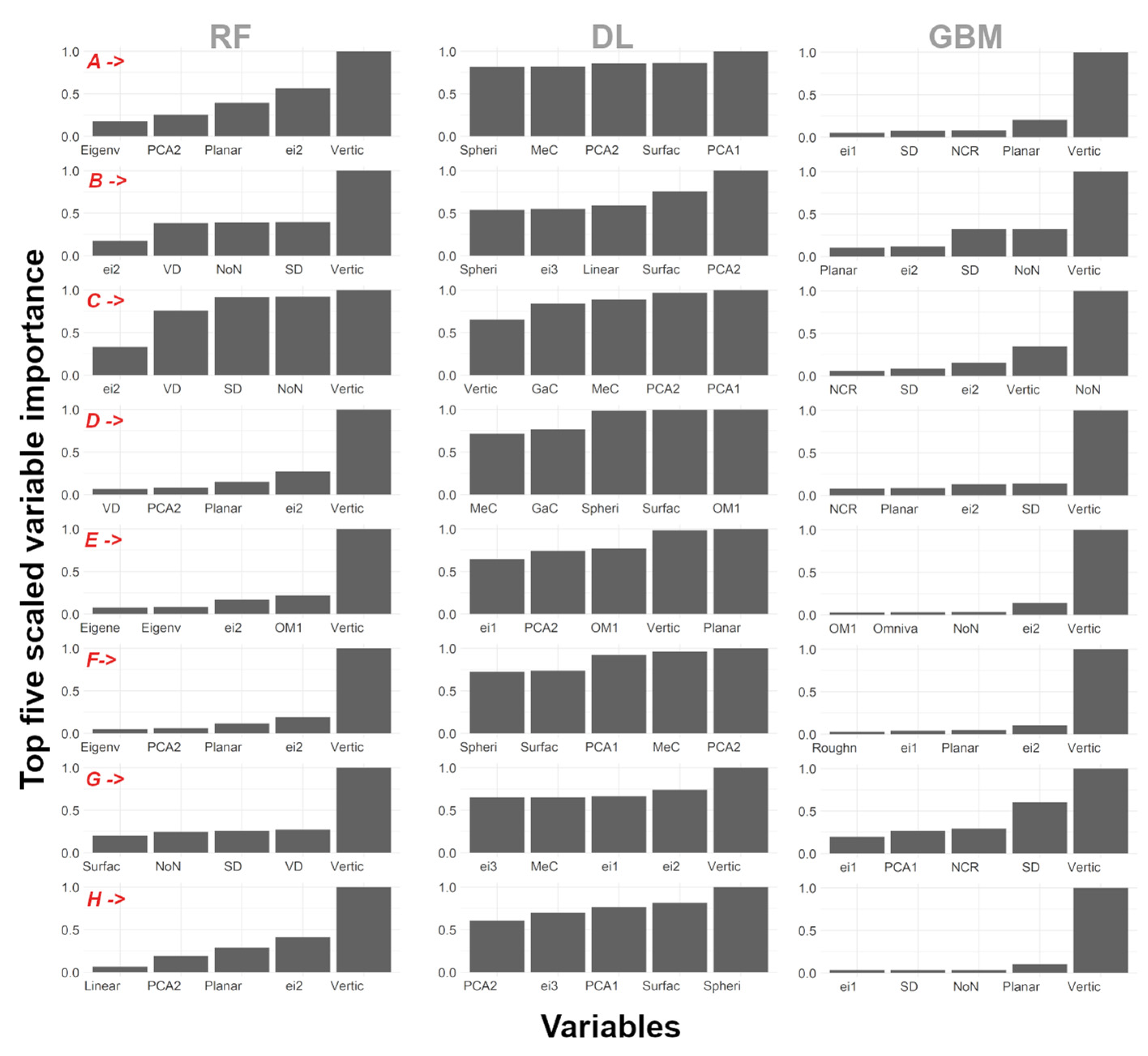
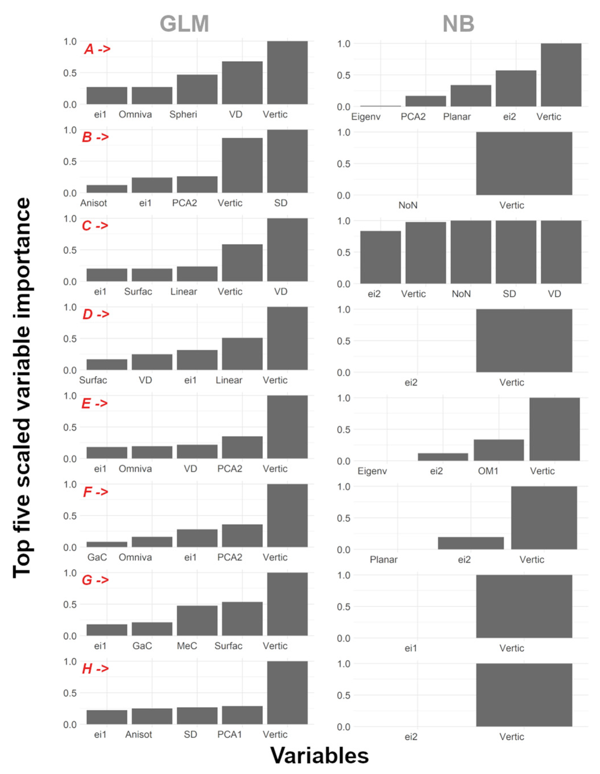
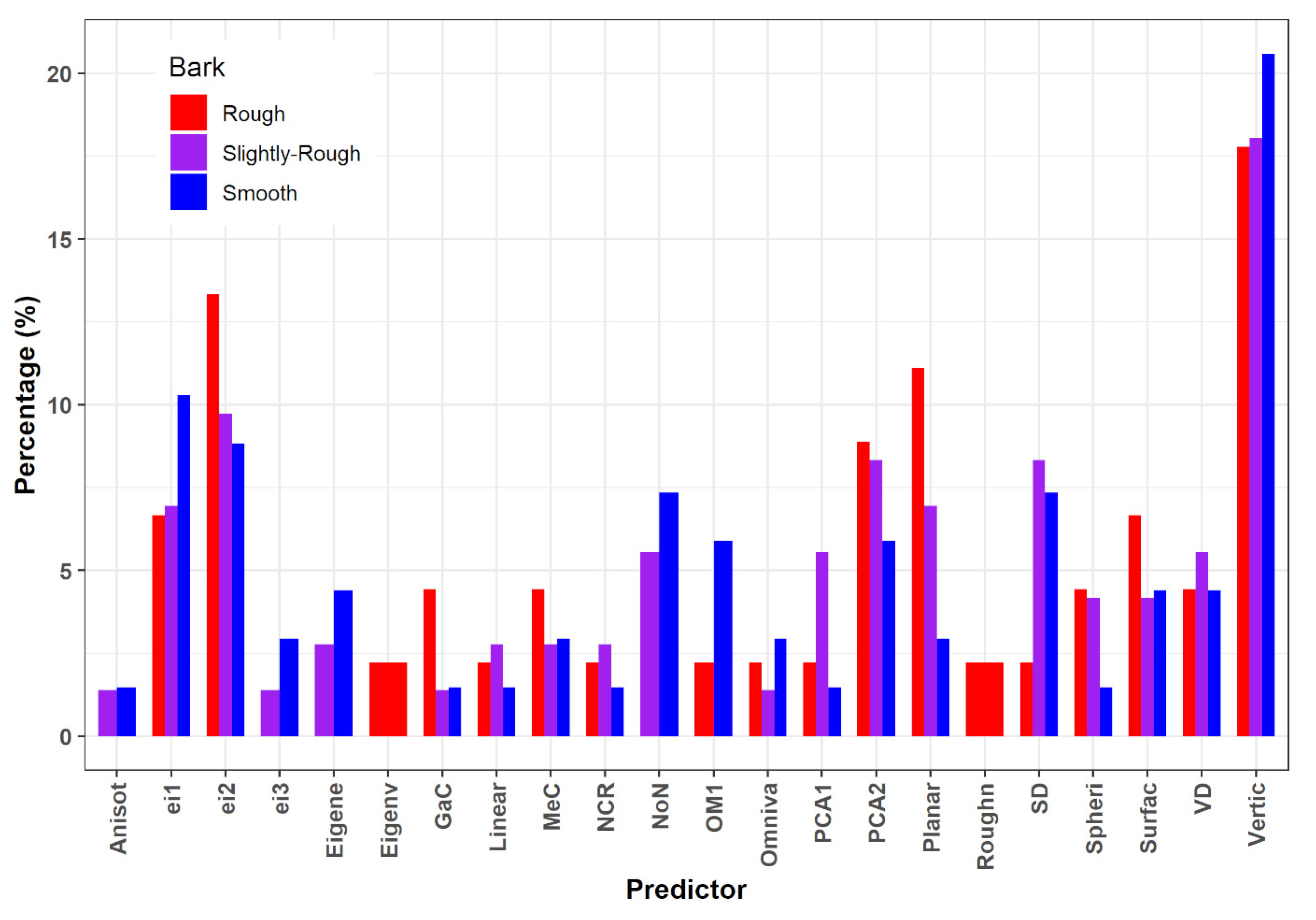
3.4. Predictor Ranking Contribution to Timber–Leaf Discrimination

The average number of predictors for implementing the algorithms ranged from 4 to 20 (Table 8). Overall, GBM- and RF-derived models required an average number of predictors ranging between 15 and 17 predictors to build their best models to discriminate timber–leaf points (Table 8). Top-performing DL-derived models required a slightly higher number of predictors than GBM- and RF-derived models: precisely 20 predictors. Finally, the top-performing GLM- and NB-derived models required fewer predictors (less than eight units) to optimize their models for the timber–leaf discrimination. In contrast, top-performing EN-derived models used all 22 predictors due to these combined top-performing RF-, DL-, GBM-, NB-, and GLM-derived models.
A similar number of predictors was required for constructing optimal models in both binary-class and multi-class classifications (Table 9), as evidenced by RF- and GLM-derived models. By contrast, the DL-derived models demanded more predictors for optimizing the best models in multi-class classifications (22 predictors) compared to binary-class classifications (9 predictors). Conversely, GBM-derived models needed slightly more predictors in the binary-class classifications (21 predictors) than in multi-class classifications (16 predictors).
Among the 22 geometry-based features tested, the ‘verticality’, ‘1st and 2nd eigenvalues’, ‘principal component analysis 1’, ‘planarity,’ and ‘surface density’ were the most recurrent and significant predictors used for all models, as supported by the top-five most important predictors used for RF, DL, GBM, GLM, and NB algorithms (see Figure 6 and Figure 7).
The variable importance analysis revealed distinct combinations of predictors across the eight tree species. The structure of the best models for IM, for instance, demonstrated a strong dependence on ‘verticality’, ‘planarity’, and ‘principal component analysis 2’ predictors in the context of the binary-class classification (Figure 7). Similarly, for TO, HO, and EHH, ‘verticality’ played a significant role in constructing the best models, combined with ‘2nd eigenvalues’ for TO, ‘number of neighbors’ and ‘surface density’ for HO, and ‘volume density’, ‘number of neighbors’, and ‘2nd eigenvalues’ for EHH.
Grouping the top-five predictors into smooth, rough, and slightly rough bark traits confirmed that ‘verticality’ was the most important predictor for trees with different bark traits (Figure 8). However, ‘sum of eigenvalues’, ‘gaussian curvature’, ‘mean curvature’, ‘planarity’, ‘roughness’, ‘sphericity’, and ‘surface variation’ were more significant to the binary-class classification of trees characterized by rough bark traits. In contrast, ‘anisotropy’, ‘1st and 3rd eigenvalues’, ‘number of neighbors’, and ‘1st-order moment’ were more relevant predictors for ML-derived models of trees characterized by smooth bark traits. Conversely, the predictors, such as ‘principal components’ and ‘surface density’, were more influential in models discriminating points on trees characterized by a slightly rough bark.

3.5. Computing Time for Model Optimization and Best Model Implementation

Our findings reveal significant variations in the computing time for optimizing the models, ranging from 1 to 908 s, and for implementing the best models, ranging from 1 to 203 s (Table 10). Indeed, these results confirm that the computational time required for model optimization exceeds that of implementing the best model.
Regarding the binary-class classification results, the GBM-, RF-, and DL-derived models exhibit greater time consumption across eight individual tree species, with DL-derived models recording times of up to approximately 908 s. The combined tree species datasets presented a similar response pattern for binary-class and multi-class classification steps.
The computation time required for configuring the models in both steps (model optimization and best model implementation) using GLM- and NB-derived models was significantly lower than that of the other four algorithms. However, optimizing the GLM-derived models for the multi-class classification required up to 10-times more time than for the binary-class classification. The best EN-derived models were seven-times more time-consuming in the multi-class than in binary-class classifications.
The time required by the top-performing ML-derived models to classify 2 million points ranged from 8 and 37 s. Specifically, the computation times were as follows: NB = 8 s, DL = 8 s; GLM= 10 s; GBM = 18 s; RF = 24 s; and EN = 37 s (Figure 9).

4. Discussion

4.1. Algorithms, Datasets, and Binary- and Multi-Class Classification Factors Influencing Timber–Leaf Discrimination

The 60 ML-derived models allowed for the accurate discrimination of timber and leaf components using individual and combined tree species datasets. The top-performing RF-, GBM-, and EN-derived models achieved the highest F1 score accuracy of 0.97 (corresponding to 0.95 of OA), making them more effective. Our results align with the outcomes obtained for other classification topics, especially those focusing on point classification [34]. Specifically, our F1 scores surpassed those obtained for similar broadleaf tree species. For example, the study of Hui et al. [63] revealed F1 scores ranging between 0.588 (wood) and 0.928 (leaf) for broadleaf trees. Similarly, Moorthy et al. [27] achieved F1 scores ranging from 0.80 (wood) to 0.97 (leaf) across various species, such as Norway maple, common alder, silver birch, and SLL trees. In another investigation, Hui et al. [64] obtained F1 scores ranging from 0.806 and 0.795 for sugar maple. When considering alternative evaluation criteria within our study, our OA results are significantly better than those obtained by Zhu et al. [62] for beech, spruce, and fir trees, who reported an average OA of 0.84; by Wei et al. [68] for Norway maple, common alder, silver birch, and small-leaved lime, who achieved an OA of 0.83; and by Wang et al. [29] for EB, coniferous trees, and SLL, who obtained values of accuracy ranging from 0.83 to 0.84. These findings demonstrate the valuable capability of these four ML algorithms to discriminate timber–leaf components in point clouds.
The EN algorithm emerges as one of the most versatile algorithms for binary-class classifications, achieving F1 scores of up to 0.97 using individual and combined tree-species datasets. While models constructed with the EN algorithm demonstrated a robust performance for half of the evaluated species, HO, EHH, TO, and HA (Table 6 and Table 7), the successful use of the EN algorithm depended on the challenges and opportunities. These included (1) higher precision for timber–leaf discrimination based on the gained information from individual algorithms; (2) sensitivity to overfitting, which depended on the choice of algorithms to assemble; (3) an improved understanding of the dataset, allowing for a more flexible exploration of the relationships between independent and dependent variables; (4) interpretability of the analysis became a challenge due to the lack of an explanation for variable importance; (5) the utilization of all predictors used in individual algorithms made it a robust model; and (6) the use of multiple algorithms increased the computational time required [69]. Nevertheless, due to its ability to combine multiple models and control overfitting estimations, this approach holds tremendous promise for classification tasks.
The robust discrimination obtained using RF- and GBM-derived models might be supported by their ability to examine large datasets, adjust the number of predictors to prevent overfitting (using the variable importance approach), robustness to outliers, and decision tree algorithms [70]. An effective dataset analysis might also be significantly aided by the learning strategy used by decision tree algorithms, which used a boosting technique involving random sampling with replacements across the weighted data [42,46]. In contrast, the DL algorithm takes advantage of artificial neural networks with multiple hidden layers to learn intricate patterns and representations from the data, emulating the analysis performed by the human brain [71].
Based on the Kappa results, our analysis demonstrates a moderate/substantial agreement between the observed and predicted data across the binary-class and multi-class classification models (ranging from 0.46 for combined tree-species datasets to 0.73 for individual tree species, respectively) (Table 6 and Table 7). Even though our Kappa results reveal a substantial agreement, these are consistent with those obtained by other researchers. For instance, Hui et al. [64] obtained a 0.60 kappa value for the sugar maple point cloud classification using the mean shift segmentation algorithm. Furthermore, the Lewos_NoRegu, Lewos_regu, and CANUPO methods obtained Kappa values of 0.66, 0.75, and 0.63, respectively, for nine coniferous and broadleaf tree species in their investigations [64]. Similar Kappa values were observed in other investigations, with a value of 0.80 obtained for green ash [30] and a range between 0.52 and 0.76 recorded for Norway maple, black alder, silver birch, and SLL tree species [26].
The literature reveals that the factors influencing Cohen’s Kappa index include the sample size, number of categories, distribution of classes, rater bias, and ambiguity in the categorical datasets [67]. However, the training and testing dataset labels were well-balanced in this study. Each point within the core points was randomly selected, and points with NA values for geometry-based features within the core points were removed. In this study, the primary factor that may have negatively influenced the quality of the Kappa index was the incorrect geometry-based characterization of points resulting from secondary factors. Specifically, these factors included (1) misclassification of points in small branches and leaves or between roughness and smoothness bark features, (2) occurrence of noise on trunks infested by lichens and lianas, (3) bark defects (e.g., knots and microhabitats), and (4) the relatively low point density captured by trees (less than 1 million points, compared to over 2 million in other studies) [12,20,62,68]. Therefore, future researchers should consider these factors in their point categorization examination. Indeed, despite our findings being good enough for most forestry purposes, a better classification may be required for other study cases, such as ecological or wood technology studies [72]. This study employed an automatic geometry-based approach embedded in CloudCompare software to characterize the points. Since we recognized that the accurate characterization of points depended on the detection of the optimal local neighborhood radius (which was automatically provided by CloudCompare software), our results confirm the feasibility and effectiveness of this approach [21,26,34,68].
Our findings indicate that model optimization requires more time than the best model implementation, which is expected due to hyperparameter tuning involving multiple attempts to find optimal combinations and predictors. However, since time efficiency was crucial, this study took advantage of HPC tools, well known for their remarkable parallel processing and accelerated computations, to reduce these time needs successfully.
The computing time findings for the binary-class classification of 2 million points display speed values ranging from 8 to 37 s (Figure 7). The results are better or aligned with those reported in other studies (Table 1) [26,29]. Additional findings also support the idea that the point density and computing training time are unrelated. However, we observed that the point quality in our study aligned with the values reported in other studies [14,20,29,40,62]. Therefore, the speed achieved by our ML-derived models using parallel computing approaches was optimal [29,73]. This result suggests that our approach can be applied to point clouds acquired at the stand level, with the entire discrimination process requiring only a few minutes. This implies that our findings may enhance the use of these technologies in forest inventories, thus contributing to the operational use of TLS in forest policy and management practices. Despite the contrasting F1 scores and OA results in the multi-class and binary-class classifications, the observed commission and omission error patterns displayed in Figure 5 allow us to assume that the multi-class classification is not a reliable method for matching top-performing ML-derived models with tree species. The same results, however, emphasize the significance of this approach for other classification tasks, such as tree-species categorization and other ecological metric evaluations [41,74].

4.2. Key Factors Hindering Accurate Binary-Class Classifications

Our findings reveal a distinct pattern of responses among different species, specifically between IM, EB, HA, and SLL, and HO, EHH, TO, and EA (Table 6). All eight tree species were categorized into rough, smooth, and slightly rough to assess the different bark surfaces. Our findings allow us to assume that the bark surface can influence the binary-class classification of points. For example, the IM tree species possesses a smooth trunk bark with few cracks, especially in mature trees, and their leaves are three-lobed with a notched leaf edge. On the contrary, TO tree species possess a bark with fissures in mature trees, and either simple or pointed lobes characterize their leaves. Conversely, HO trees exhibit a smooth trunk bark and their leaves are round to oval in shape, doubly toothed, hairy, and pointed at the tip (https://www.actaplantarum.org/; accessed on 9 September 2023) [26]. Discriminating points for trees characterized by a rough bark required the detection of geometries that described the curvature among the closest 3D points, mainly the verticality, followed by secondary geometries, such as the sum of eigenvalues, roughness, Gaussian curvature, mean curvature, and planarity. On the other hand, the discrimination of points for trees characterized by a smooth bark required geometries that described the cohesion of the closest 3D points, including anisotropy, 3rd eigenvalues, eigenentropy, number of neighbors, and 1st-order moment. However, certain geometries were commonly used for discriminating points across trees with different bark traits, such as the eigenvalues and the 1st and 2nd principal component analyses. Nevertheless, our results also reveal that top-performing models developed using six ML algorithms can regulate the factor of tree species during the model optimization step at the cost of increasing the predictors or changing the predictor combinations (Table 5, Figure 6 and Figure 7).
Nevertheless, the timber–leaf discrimination can also be influenced by other factors, as previously mentioned (i.e., noise occurrence and bark surface), technical and operational aspects, and forest structure (i.e., DBH and TH) [12]. Some secondary hindering factors undoubtedly contributed to the distinct pattern of responses observed across the tree species. These factors included occlusions from small trees or shrubs on large branches (blocked the pass of the laser from the TLS instrument to branch), the reduced accuracy of laser beams in the intermediate and overstory layers (our trees reached heights of up to 30 m), specific bark surface of mature trees, and stem density (672 tree ha−1) [26,27,28,29]. Operational factors, such as forest canopy conditions (leaf-off) during TLS data collection and technical aspects during the acquisition of TLS data can also affect the point characterization. However, these factors can be overcome by following the standard protocols. In this study, TLS data were collected in an uneven-aged and multi-layered mixed-tree species, with more than ten tree species, which was not an accessible area for this kind of instrument. Given these specific forest conditions, further research can be beneficial to calibrate our method for different forest types. As a result, this will provide valuable insights into the potential of machine learning for accurately discriminating timber and leaves across various tree species.

5. Conclusions

This study evaluated the effectiveness of ML-derived models in discriminating leaves from timber components in eight Mediterranean tree species. The findings highlight the superior performances of the RF-, GBM-, EN-, and DL-derived models among the ML-derived models. Moreover, using individual tree species datasets was revealed to be more determinant for the discriminant task problem than combined tree-species datasets. However, combining the datasets highlighted the EN method’s versatility for better discriminating large datasets and multiple classes.
Our results show contrasting responses between the binary-class and multi-class classification strategies. While the binary-class classification excelled in its overall accuracy and Kappa values, the multi-class classification indicated dominant F1 scores and precision. Due to frequent omission and commission errors, the multi-class outcome did not provide sufficient information to determine the preferred algorithm for each tree species. This finding underscores the importance of selecting an appropriate classification approach and dataset aligned with specific objectives. Our results highlight the crucial role of several factors, ranging from phenotypic factors, such as bark surface (i.e., roughness and smoothness), technical issues (noise points), and structural components, in the binary-class classification problem. Therefore, this study provides valuable information to readers for the binary-class classification challenges and lays the foundation for future work to improve the use of point classification accuracy in complex circumstances.
In conclusion, this study presents a multi-dimensional analysis that underlines the best ML algorithms, dataset considerations, classification approaches, and significant variables in discriminating between timber and leaves. Moreover, our findings represent the essential advancement for accurately assessing ecological indicators, such as vegetation indices. Further investigations are necessary to calibrate the developed models for other species and to implement them at the forest stand level.

Author Contributions

Conceptualization, C.A., G.S. and B.L.; methodology, C.A., G.S. and B.L.; validation, C.A.; data curation, C.A., G.S. and B.L.; writing—original draft preparation, C.A., G.S. and J.A.M.-V.; writing—review and editing, C.A., G.S., M.M. (Mauro Maesano), M.M. (Marco Marchetti) and J.A.M.-V.; visualization, C.A.; supervision, M.M. (Marco Marchetti) and B.L.; project administration, M.M. (Marco Marchetti) and B.L.; funding acquisition, B.L. All authors have read and agreed to the published version of the manuscript.

Funding

This research received no external funding.

Data Availability Statement

Not applicable.

Acknowledgments

This research was supported by the Establishing Urban FORest-based solutions In Changing Cities (EUFORICC) project.

Conflicts of Interest

The authors declare no conflict of interest.

Appendix A

The training (70%) and testing (30%) point clouds used for the discrimination classification approach (Figure A1).
Figure A1. Frequency of observation for training and testing data separated by class (leaf and wood).
Remotesensing 15 04450 g0a1

References

  1. Millennium Ecosystem Assessment. In Ecosystems and Human Well-Being: Synthesis; Island Press: Washington, DC, USA, 2005.
  2. Chirici, G.; Barbati, A.; Maselli, F. Modelling of Italian forest net primary productivity by the integration of remotely sensed and GIS data. For. Ecol. Manag. 2007, 246, 285–295. [Google Scholar] [CrossRef]
  3. McRoberts, R.E.; Tomppo, E.O. Remote sensing support for national forest inventories. Remote Sens. Environ. 2007, 110, 412–419. [Google Scholar] [CrossRef]
  4. Dassot, M.; Constant, T.; Fournier, M. The use of terrestrial LiDAR technology in forest science: Application fields, benefits and Challenges The use of terrestrial LiDAR technology in forest science: Application fields benefits and challenges. Ann. For. Sci. 2011, 68, 959–974. [Google Scholar] [CrossRef]
  5. Liang, X.; Wang, Y.; Pyörälä, J.; Lehtomäki, M.; Yu, X.; Kaartinen, H.; Kukko, A.; Honkavaara, E.; Issaoui, A.E.I.; Nevalainen, O.; et al. Forest in situ observations using unmanned aerial vehicle as an alternative of terrestrial measurements. For. Ecosyst. 2019, 6, 20. [Google Scholar] [CrossRef]
  6. Saarinen, N.; Kankare, V.; Vastaranta, M.; Luoma, V.; Pyörälä, J.; Tanhuanpää, T.; Liang, X.; Kaartinen, H.; Kukko, A.; Jaakkola, A.; et al. Feasibility of Terrestrial laser scanning for collecting stem volume information from single trees. ISPRS J. Photogramm. Remote Sens. 2017, 123, 140–158. [Google Scholar] [CrossRef]
  7. Liang, X.; Hyyppä, J.; Kaartinen, H.; Lehtomäki, M.; Pyörälä, J.; Pfeifer, N.; Holopainen, M.; Brolly, G.; Francesco, P.; Hackenberg, J.; et al. International benchmarking of terrestrial laser scanning approaches for forest inventories. ISPRS J. Photogramm. Remote Sens. 2018, 144, 137–179. [Google Scholar] [CrossRef]
  8. Torresan, C.; Berton, A.; Carotenuto, F.; Di Gennaro, S.F.; Gioli, B.; Matese, A.; Miglietta, F.; Vagnoli, C.; Zaldei, A.; Wallace, L. Forestry applications of UAVs in Europe: A review. Int. J. Remote Sens. 2017, 38, 2427–2447. [Google Scholar] [CrossRef]
  9. Næsset, E. Predicting forest stand characteristics with airborne scanning laser using a practical two-stage procedure and field data. Remote Sens. Environ. 2001, 80, 88–99. [Google Scholar] [CrossRef]
  10. Pfeifer, N.; Gorte, B.; Winterhalder, D. Automatic reconstruction of single trees from terrestrial laser scanner data. In Proceedings of the 20th ISPRS Congress, Istanbul, Turkey, 12–23 July 2004; Volume 35, pp. 114–119. [Google Scholar]
  11. Alvites, C.; Marchetti, M.; Lasserre, B.; Santopuoli, G. LiDAR as a Tool for Assessing Timber Assortments: A Systematic Literature Review. Remote Sens. 2022, 14, 4466. [Google Scholar] [CrossRef]
  12. Alvites, C.; Santopuoli, G.; Hollaus, M.; Pfeifer, N.; Maesano, M.; Moresi, F.V.; Marchetti, M.; Lasserre, B. Terrestrial laser scanning for quantifying timber assortments from standing trees in a mixed and multi-layered mediterranean forest. Remote Sens. 2021, 13, 4265. [Google Scholar] [CrossRef]
  13. Calders, K.; Adams, J.; Armston, J.; Bartholomeus, H.; Bauwens, S.; Bentley, L.P.; Chave, J.; Danson, F.M.; Demol, M.; Disney, M.; et al. Terrestrial laser scanning in forest ecology: Expanding the horizon. Remote Sens. Environ. 2020, 251, 112102. [Google Scholar] [CrossRef]
  14. Wang, D.; Hollaus, M.; Pfeifer, N. Feasibility of machine learning methods for separating wood and leaf points from terrestrial laser scanning data. ISPRS Ann. Photogramm. Remote Sens. Spat. Inf. Sci. 2017, 4, 157–164. [Google Scholar] [CrossRef]
  15. Hackenberg, J.; Spiecker, H.; Calders, K.; Disney, M.; Raumonen, P. SimpleTree—An efficient open source tool to build tree models from TLS clouds. Forests 2015, 6, 4245–4294. [Google Scholar] [CrossRef]
  16. Montoya, O.; Icasio-Hernández, O.; Salas, J. TreeTool: A tool for detecting trees and estimating their DBH using forest point clouds. SoftwareX 2021, 16, 100889. [Google Scholar] [CrossRef]
  17. Molina-Valero, J.A.; Martínez-Calvo, A.; Ginzo Villamayor, M.J.; Novo Pérez, M.A.; Álvarez-González, J.G.; Montes, F.; Pé-rez-Cruzado, C. Operationalizing the use of TLS in forest inventories: The R package FORTLS. Environ. Model. Softw. 2022, 150, 105337. [Google Scholar] [CrossRef]
  18. Terryn, L.; Calders, K.; Åkerblom, M.; Bartholomeus, H.; Disney, M.; Levick, S.; Origo, N.; Raumonen, P.; Verbeeck, H. An-alysing individual 3D tree structure using the R package ITSMe. Methods Ecol. Evol. 2022, 2022, 231–241. [Google Scholar] [CrossRef]
  19. Yun, T.; An, F.; Li, W.; Sun, Y.; Cao, L.; Xue, L. A novel approach for retrieving tree leaf area from ground-based LiDAR. Remote Sens. 2016, 8, 942. [Google Scholar] [CrossRef]
  20. Zhou, J.; Wei, H.; Zhou, G.; Song, L. Separating leaf andwood points in terrestrial laser scanning data using multiple optimal scales. Sensors 2019, 19, 1852. [Google Scholar] [CrossRef]
  21. Weinmann, M.; Urban, S.; Hinz, S.; Jutzi, B.; Mallet, C. Distinctive 2D and 3D features for automated large-scale scene analysis in urban areas. Comput. Graph. 2015, 49, 47–57. [Google Scholar] [CrossRef]
  22. Ferrara, R.; Virdis, S.G.P.; Ventura, A.; Ghisu, T.; Duce, P.; Pellizzaro, G. An automated approach for wood-leaf separation from terrestrial LIDAR point clouds using the density based clustering algorithm DBSCAN. Agric. For. Meteorol. 2018, 262, 434–444. [Google Scholar] [CrossRef]
  23. Yang, L.; Shami, A. On hyperparameter optimization of machine learning algorithms: Theory and practice. Neurocomputing 2020, 415, 295–316. [Google Scholar] [CrossRef]
  24. Wang, D.; Momo Takoudjou, S.; Casella, E. LeWoS: A universal leaf-wood classification method to facilitate the 3D modelling of large tropical trees using terrestrial LiDAR. Methods Ecol. Evol. 2020, 11, 376–389. [Google Scholar] [CrossRef]
  25. Stovall, A.E.L.; Masters, B.; Fatoyinbo, L.; Yang, X. TLSLeAF: Automatic leaf angle estimates from single-scan terrestrial laser scanning. New Phytol. 2021, 232, 1876–1892. [Google Scholar] [CrossRef]
  26. Vicari, M.B.; Disney, M.; Wilkes, P.; Burt, A.; Calders, K.; Woodgate, W. Leaf and wood classification framework for terrestrial LiDAR point clouds. Methods Ecol. Evol. 2019, 10, 680–694. [Google Scholar] [CrossRef]
  27. Moorthy, S.M.K.; Calders, K.; Vicari, M.B.; Verbeeck, H. Improved Supervised Learning-Based Approach for Leaf and Wood Classification from LiDAR Point Clouds of Forests. IEEE Trans. Geosci. Remote Sens. 2020, 58, 3057–3070. [Google Scholar] [CrossRef]
  28. Tan, K.; Zhang, W.; Dong, Z.; Cheng, X.; Cheng, X. Leaf and Wood Separation for Individual Trees Using the Intensity and Density Data of Terrestrial Laser Scanners. IEEE Trans. Geosci. Remote Sens. 2021, 59, 7038–7050. [Google Scholar] [CrossRef]
  29. Wang, D.; Brunner, J.; Ma, Z.; Lu, H.; Hollaus, M.; Pang, Y.; Pfeifer, N. Separating tree photosynthetic and non-photosynthetic components from point cloud data using Dynamic Segment Merging. Forests 2018, 9, 252. [Google Scholar] [CrossRef]
  30. Sun, J.; Wang, P.; Gao, Z.; Liu, Z.; Li, Y.; Gan, X.; Liu, Z. Wood–leaf classification of tree point cloud based on intensity and geometric information. Remote Sens. 2021, 13, 4050. [Google Scholar] [CrossRef]
  31. Tan, K.; Ke, T.; Tao, P.; Liu, K.; Duan, Y.; Zhang, W.; Wu, S. Discriminating Forest Leaf and Wood Components in TLS Point Clouds at Single-Scan Level Using Derived Geometric Quantities. IEEE Trans. Geosci. Remote Sens. 2022, 60, 5701517. [Google Scholar] [CrossRef]
  32. Xi, Z.; Hopkinson, C.; Rood, S.B.; Peddle, D.R. See the forest and the trees: Effective machine and deep learning algorithms for wood filtering and tree species classification from terrestrial laser scanning. ISPRS J. Photogramm. Remote Sens. 2020, 168, 1–16. [Google Scholar] [CrossRef]
  33. Wang, L.; Meng, W.; Xi, R.; Zhang, Y.; Ma, C.; Lu, L.; Zhang, X. 3D point cloud analysis and classification in large-scale scene based on deep learning. IEEE Access 2019, 7, 55649–55658. [Google Scholar] [CrossRef]
  34. Hackel, T.; Wegner, J.D.; Schindler, K. Fast Semantic Segmentation of 3D Point Clouds with Strongly Varying Density. ISPRS Ann. Photogramm. Remote Sens. Spat. Inf. Sci. 2016, 3, 177–184. [Google Scholar] [CrossRef]
  35. Wang, D. Unsupervised semantic and instance segmentation of forest point clouds. ISPRS J. Photogramm. Remote Sens. 2020, 165, 86–97. [Google Scholar] [CrossRef]
  36. Barbati, A.; Marchetti, M.; Chirici, G.; Corona, P. European Forest Types and Forest Europe SFM indicators: Tools for monitoring progress on forest biodiversity conservation. For. Ecol. Manag. 2014, 321, 145–157. [Google Scholar] [CrossRef]
  37. Santopuoli, G.; Di Cristofaro, M.; Kraus, D.; Schuck, A.; Lasserre, B.; Marchetti, M. Biodiversity conservation and wood pro-duction in a Natura 2000 Mediterranean forest. A trade-off evaluation focused on the occurrence of microhabitats. iForest Biogeosci. For. 2019, 12, 76–84. [Google Scholar] [CrossRef]
  38. Alvites, C.; Santopuoli, G.; Maesano, M.; Chirici, G.; Moresi, F.V.; Tognetti, R.; Marchetti, M.; Lasserre, B. Unsupervised al-gorithms to detect single trees in a mixed-species and multi-layered Mediterranean forest using LiDAR data. Can. J. For. Res. 2021, 51, 1766–1780. [Google Scholar] [CrossRef]
  39. Hackel, T.; Wegner, J.D.; Schindler, K. Contour detection in unstructured 3D point clouds. In Proceedings of the IEEE conference on computer vision and pattern recognition, Las Vegas, NV, USA, 26 June–1 July 2016; pp. 1610–1618. [Google Scholar] [CrossRef]
  40. Wu, B.; Zheng, G.; Chen, Y. An improved convolution neural network-based model for classifying foliage and woody components from terrestrial laser scanning data. Remote Sens. 2020, 12, 1010. [Google Scholar] [CrossRef]
  41. Abed, S.H.; Al-Waisy, A.S.; Mohammed, H.J.; Al-Fahdawi, S. A modern deep learning framework in robot vision for automated bean leaves diseases detection. Int. J. Intell. Robot. Appl. 2021, 5, 235–251. [Google Scholar] [CrossRef] [PubMed]
  42. Breiman, L. Random forests. Mach. Learn. 2001, 45, 5–32. [Google Scholar] [CrossRef]
  43. Suzuki, K.; Suzuki, K. Artificial Neural Networks: Methodological Advances and Biomedical Applications; BoD–Books on Demand; Suzuki: Hamamatsu, Japan, 2011; ISBN 9789533072432. [Google Scholar]
  44. Abiodun, O.I.; Jantan, A.; Omolara, A.E.; Dada, K.V.; Mohamed, N.A.E.; Arshad, H. State-of-the-art in artificial neural network applications: A survey. Heliyon 2018, 4, e00938. [Google Scholar] [CrossRef] [PubMed]
  45. Friedman, J.H. Greedy Function Approximation: A Gradient Boosting Machine. Ann. Stat. 2001, 29, 1189–1232. [Google Scholar] [CrossRef]
  46. Natekin, A.; Knoll, A. Gradient boosting machines, a tutorial. Front. Neurorobot. 2013, 7, 21. [Google Scholar] [CrossRef]
  47. Nelder, J.A.; Wedderburn, R.W.M. Generalized linear models. J. Royral Stat. Soc. 1972, 135, 370–384. [Google Scholar] [CrossRef]
  48. McCullagh, P. Generalized Linear Models; Routledge: Abingdon, UK, 2019. [Google Scholar]
  49. Rish, I. An empirical study of the naive bayes classifier. In Proceedings of the IJCAI 2001 Workshop on Empirical Methods in Artificial Intelligence, Seattle, WA, USA, 4–6 August 2001; Volume 3, pp. 41–46. [Google Scholar] [CrossRef]
  50. Marcot, B.G.; Steventon, J.D.; Sutherland, G.D.; McCann, R.K. Guidelines for developing and updating Bayesian belief net-works applied to ecological modeling and conservation. Can. J. For. Res. 2006, 36, 3063–3074. [Google Scholar] [CrossRef]
  51. Breiman, L. Stacked regressions. Mach. Learn. 1996, 24, 49–64. [Google Scholar] [CrossRef]
  52. Roussel, J.R.; Auty, D.; Coops, N.C.; Tompalski, P.; Goodbody, T.R.H.; Meador, A.S.; Bourdon, J.F.; de Boissieu, F.; Achim, A. lidR: An R package for analysis of Airborne Laser Scanning (ALS) data. Remote Sens. Environ. 2020, 251, 112061. [Google Scholar] [CrossRef]
  53. Wickham, H.; Francois, R.; Lionel, H.; Müller, K.; Vaughan, D.; Software, P. Dplyr: A Grammar of Data Manipulation. R Package Version 1.1.2. 2023. Available online: https://github.com/tidyverse/dplyr (accessed on 10 June 2023).
  54. Aiello, S.; Eckstrand, E.; Fu, A.; Landry, M.; Aboyoun, P. Machine Learning with R and H2O. 2016. Available online: https://h2o-release.s3.amazonaws.com/h2o/master/3283/docs-website/h2o-docs/booklets/R_Vignette.pdf (accessed on 20 August 2023).
  55. Kuhn, M. Building predictive models in R using the caret package. J. Stat. Softw. 2008, 28, 1–26. [Google Scholar] [CrossRef]
  56. Majka, A.M.; Majka, M.M. Package ‘Naivebayes’. 2020. Available online: https://cloud.r-project.org/web/packages/naivebayes/naivebayes.pdf (accessed on 10 June 2023).
  57. Weston, S.; Calaway, R.; Ooi, H.; Daniel, F. Package ‘Foreach’. Version 1.5.2. Available online: https://github.com/RevolutionAnalytics/foreach (accessed on 10 June 2023).
  58. Shpakovych, M. Optimization and Machine Learning Algorithms Applied to the Phase Control of an Array of Laser Beams Maksym Shpakovych to Cite This Version: HAL Id: Tel-03941758 e des Sciences et Techniques These Optimization and Machine Learning Algorithms Applied. 2023. Optimization and Control [math.OC]. Université de Limoges, 2022. English. NNT: 2022LIMO0120. Available online: https://theses.hal.science/ (accessed on 9 September 2023).
  59. Berrar, D. Bayes’ theorem and naive bayes classifier. Encycl. Bioinform. Comput. Biol. ABC Bioinform. 2018, 403, 412. [Google Scholar] [CrossRef]
  60. Zuur, A.F.; Ieno, E.N.; Elphick, C.S. A protocol for data exploration to avoid common statistical problems. Methods Ecol. Evol. 2010, 1, 3–14. [Google Scholar] [CrossRef]
  61. Ripley, B.; Venables, W.; Ripley, M.B. Package ‘Nnet’. R Package Version. 2016. Available online: https://staff.fmi.uvt.ro/~daniela.zaharie/dm2019/RO/lab/lab3/biblio/nnet.pdf (accessed on 9 September 2023).
  62. Zhu, X.; Skidmore, A.K.; Darvishzadeh, R.; Niemann, K.O.; Liu, J.; Shi, Y.; Wang, T. Foliar and woody materials discriminated using terrestrial LiDAR in a mixed natural forest. Int. J. Appl. Earth Obs. Geoinf. 2018, 64, 43–50. [Google Scholar] [CrossRef]
  63. Hui, Z.; Xia, Y.; Nie, Y.; Chang, Y.; Hu, H.; Li, N.; He, Y. Fractal Dimension Based Supervised Learning for Wood and Leaf Classification from Terrestrial Lidar Point Clouds. ISPRS Ann. Photogramm. Remote Sens. Spat. Inf. Sci. 2020, 5, 95–99. [Google Scholar] [CrossRef]
  64. Hui, Z.; Jin, S.; Xia, Y.; Wang, L.; Yevenyo Ziggah, Y.; Cheng, P. Wood and leaf separation from terrestrial LiDAR point clouds based on mode points evolution. ISPRS J. Photogramm. Remote Sens. 2021, 178, 219–239. [Google Scholar] [CrossRef]
  65. Robin, X.A.; Turck, N.; Hainard, A.; Tiberti, N.; Lisacek, F.; Sanchez, J.-C.; Muller, M.J. pROC: An open-source package for R and S+ to analyze and compare ROC curves. BMC Bioinform. 2011, 12, 77. [Google Scholar] [CrossRef] [PubMed]
  66. Wickham, H.; Vaughan, D.; Girlich, M.; Ushey, K.; PBC, Posit. Package ‘Tidyr’. Version 1.3.0. Available online: https://tidyr.tidyverse.org (accessed on 10 June 2023).
  67. Sun, S. Meta-analysis of Cohen’s kappa. Health Serv. Outcomes Res. Methodol. 2011, 11, 145–163. [Google Scholar] [CrossRef]
  68. Wei, H.; Zhou, G.; Zhou, J. Comparison of single and multi-scale method for leaf and wood points classi-fication from terrestrial laser scanning data. ISPRS Ann. Photogramm. Remote Sens. Spat. Inf. Sci. 2018, 4, 217–223. [Google Scholar] [CrossRef]
  69. Martinez-Gil, J. A comprehensive review of stacking methods for semantic similarity measurement. Mach. Learn. Appl. 2022, 10, 100423. [Google Scholar] [CrossRef]
  70. Kotsiantis, S.B. Decision trees: A recent overview. Artif. Intell. Rev. 2013, 39, 261–283. [Google Scholar] [CrossRef]
  71. Ojha, V.K.; Abraham, A.; Sná, V. Metaheuristic design of feedforward neural networks: A review of two decades of research. Eng. Appl. Artif. Intell. 2017, 60, 97–116. [Google Scholar]
  72. Rehush, N.; Abegg, M.; Waser, L.T.; Brändli, U. Identifying Tree-Related Microhabitats in TLS Point Clouds Using Machine Learning. Remote Sens. 2018, 10, 1735. [Google Scholar] [CrossRef]
  73. Kane, M.J.; Emerson, J.W.; Weston, S. Scalable strategies for computing with massive data. J. Stat. Softw. 2013, 55, 1–19. [Google Scholar] [CrossRef]
  74. Wen, H.; Zhou, X.; Zhang, C.; Liao, M.; Xiao, J. Different-Classification-Scheme-Based Machine Learning Model of Building Seismic Resilience Assessment in a Mountainous Region. Remote Sens. 2023, 15, 2226. [Google Scholar] [CrossRef]
Figure 1. Location of the study area (red point in box (A)). Example of TLS point clouds (B) and the frequency of the tree species composition in the study area in relation to a total of 178 trees (C).
Remotesensing 15 04450 g001
Figure 2. Workflow implemented for discriminating timber from leaf components using terrestrial laser-scanning (TLS) point clouds.
Remotesensing 15 04450 g002
Figure 3. Timber–leaf point clouds for the eight tree species. A graphic representation of the discrimination of point clouds by species achieved using the best algorithms: stacked ensemble models (e.g., hornbeam, European hop-hornbeam, Turkey oak, and hazel) and gradient boosting machine (Italian maple, European beech, European ash, and small-leaf Lime). These algorithms were selected based on their F1 scores and high overall accuracy measurements.
Remotesensing 15 04450 g003
Figure 4. Confusion matrices for six machine learning algorithms in the binary-class classification task. Combined dataset labeled as timber and leaf classes used. RF (random forest), DL (deep learning), GBM (gradient boosting machine), GLM (generalized linear model), NB (naive Bayes), and EN (stacked ensemble). The color scale ranges from white to mosaic blue, representing the minimum (0) and maximum (150,000) frequency, respectively.
Remotesensing 15 04450 g004
Figure 5. Confusion matrices for six machine learning algorithms in the multi-class classification task. Combined tree species dataset labeled based on tree species and timber–leaf classes using RF (random forest), DL (deep learning), GBM (gradient boosting machine), GLM (generalized linear model), NB (naive Bayes), and EN (stacked ensemble). Leaf and wood classes were associated with corresponding tree species: IM (Italian maple), HO (hornbeam), EHH (European hop-hornbeam), TO (Turkey oak), EB (European beech), EA (European ash), HA (hazel), and SLL (small-leaf lime).
Remotesensing 15 04450 g005
Figure 6. Top-five predictors of scaled variable importance of the timber–leaf discrimination using three algorithms, random forest (RF), deep learning (DL), and GBM (gradient boosting machine), for eight tree species: (A) Italian maple, (B) hornbeam, (C) European hop-hornbeam, (D) Turkey oak, (E) European beech, (F) European ash, (G) hazel, and (H) small-leaved lime. The abbreviated geometry-based features are: anisotropy (Anisot), 1st (ei1), 2nd (ei2), and 3rd (ei3) eigenvalues, eigenentropy (Eigene), sum of eigenvalues (Eigenv), Gaussian curvature (GaC), linearity (linear), mean curvature (MeC), normal change rate (NCR), number of neighbor (NoN), 1st-order moment (OM1), omnivariance (Ommiva), principal component analysis 1 (PCA1), principal component analysis 2 (PCA2), planarity (Planar), roughness (Roughn), surface density (SD), sphericity (Spheri), surface variation (Surfac), volume density (VD), and verticality (Vertic).
Remotesensing 15 04450 g006
Figure 7. Top-five predictors of scaled variable importance of the timber–leaf discrimination using two algorithms, GLM (generalized linear model) and NB (naive Bayes), for eight tree species: (A) Italian maple, (B) hornbeam, (C) European hop-hornbeam, (D) Turkey oak, (E) European beech, (F) European ash, (G) hazel, and (H) small-leaved lime. The abbreviated geometry-based features are: anisotropy (Anisot), 1st (ei1) and 2nd (ei2) eigenvalues, sum of eigenvalues (Eigenv), Gaussian curvature (GaC), linearity (linear), mean curvature (MeC), number of neighbor (NoN), omnivariance (Ommiva), principal component analysis 1 (PCA1), principal component analysis 2 (PCA2), planarity (Planar), surface density (SD), sphericity (Spheri), surface variation (Surfac), volume density (VD), and verticality (Vertic).
Remotesensing 15 04450 g007
Figure 8. Results of the top-five predictors grouped into three groups based on tree bark characteristics: rough, smooth, and slightly rough. Percentage of predictors by each bark type. The abbreviated geometry-based features are: anisotropy (Anisot), 1st (ei1), 2nd (ei2), and 3rd (ei3) eigenvalues, eigenentropy (Eigene), the sum of eigenvalues (Eigenv), Gaussian curvature (GaC), linearity (linear), mean curvature (MeC), normal change rate (NCR), number of neighbor (NoN), 1st-order moment (OM1), omnivariance (Ommiva), principal component analysis 1 (PCA1), principal component analysis 2 (PCA2), planarity (Planar), roughness (Roughn), surface density (SD), sphericity (Spheri), surface variation (Surfac), volume density (VD), and verticality (Vertic).
Remotesensing 15 04450 g008
Figure 9. Timber–leaf points discrimination for European beech totaling 2 million points. A zoomed-in view emphasizes minor commission/omission errors. We used the best model from six machine learning algorithms: RF (random forests, DL (deep learning), GBM (gradient boosting machine), GLM (generalized linear model), NB (naive Bayes), and EN (stacked ensemble).
Remotesensing 15 04450 g009
Table 1. Computing time for binary-class classification of TLS point clouds using different hardware specifications.
IDPoint Cloud (pts)Time (s or min) Hardware SpecificationsReference
11 × 10690 sPC 64-bit Windows 10 PC, Intel® CoreTM i7-8850H, 32 GB RAM[24]
21 × 10560 sNot specified[26]
35 × 105500 sPC with Core i7 CPU 920 2.67 GHz, 3G RAM, NVIDIA GeForce GTX[33]
43 × 10890 minPC with Intel® Xeon E5-1650 CPU, 64 GB RAM[34]
51 × 10630–90 sPC 64-bit Windows 7 with an Intel® Xeon(R) E5-2609 v4 1.7
GHz processor and 32 GB RAM
[20]
61 × 10664 sPC 64-bit Windows 10,
Intel® CoreTM i7-8850H and 32 GB RAM
[35]
Table 2. Machine learning algorithms used for the binary classification of TLS (terrestrial laser-scanning) point clouds.
Machine Learning Algorithms Used for the Binary Classification
AlgorithmDescriptionReference
Random forestsAn ensemble algorithm composed of a pool of tree-structured classifiers, where every tree grows based on the training data and randomly and identically distributed random vectors, and allows a vote for the most popular input data class. RF supports both regression and classification analyses.[42]
Deep learningA mathematical model computing a set of data in a similar way to how the human brain processes information, and it is based on a multi-layer feedforward artificial neural network.[43,44]
Gradient boosting machines An ensemble machine learning algorithm developed by Friedman. The learning approach of this algorithm is based on the construction of a robust predictive model that, in turn, is trained by a sequential weak predictive model.[45,46]
Generalized linear model Encompasses conventional regression models analyzing continuous and/or categorical predictor values characterized by a normal (i.e., Gaussian) or non-normal (i.e., Poisson, binomial, and gamma) distribution.[47,48]
Naive Bayes A classifier algorithm belonging to a group of probabilistic classifiers based on the Bayes theorem. Its learning approach assumes that each feature of a set of data is independent and that such a feature belongs to a class according to the Bayesian probability.[49,50]
Stacked ensemble modelsA supervised algorithm proposing a better combination of ensemble algorithms. EN encompasses all five previous machine/deep learning algorithms through a stacked ensemble approach to generate an improved model based on their principles. The lowest cross-validation error rate selects a better combination of algorithms.[51]
Table 3. Hyperparameters set for optimizing models for RF (random forest), DL (deep learning), GBM (gradient boosting machine), and NB (naive Bayes).
IDAlgorithmHyperparameters
1RFNfolds:10
2Ntrees: From 50 to 500, by 50
3Max_depth: From 10 to 30, by 2
4Nbins: From 20 to 30, by 10
5Sample_rate: From 0.55 to 0.80, by 0.05
6Mtries: From 2 to 6, by 1
7DLNfolds:10
8Activation (type1): Rectifier and Maxout
9Hidden (type1): list(c(5, 5, 5, 5, 5), c(10, 10, 10, 10), c(50, 50, 50), c(100, 100, 100))
10Epochs (type1): From 50 to 200, by 10
11L1 (type1): c(0, 0.00001, 0.0001)
12L2 (type1): c(0, 0.00001, 0.0001)
13GBMNfolds:10
14Ntree: From 50 to 500, by 50
15Max_depth: From 10 to 30, by 2
16Sample_rate: From 0.55 to 0.80, by 0.05
17NBNfolds: 10
18Laplace: From 0 to 5, by 0.5
RF: Ntrees: number of trees in the random forest ensemble. Max_depth: maximum depth of individual trees. Nbins: number of bins used for the histogram-based computation. Affects the quality and speed of training. Mtries: number of variables randomly sampled as candidates for splitting at each tree node. Sample_rate: fraction of rows (observations) used for tree building. DL: Activation: activation mathematical function used for hidden layers (e.g., ‘Rectifier’ and ‘Maxout’). Hidden: number of neurons in hidden layers and their configurations. Epochs: number of training iterations over the dataset. L1: L1 regularization strength for controlling feature selection. L2: L2 regularization strength for controlling model complexity. GBM: Ntree: number of boosting iterations (trees) in the ensemble. Max_depth: maximum depth of individual trees. Sample_rate: fraction of rows (observations) used for building each tree. NB: Laplace: Laplace smoothing parameter is used to handle zero probabilities.
Table 4. Field and terrestrial laser-scanning (TLS) data for eight point clouds.
Tree TLS and Field Data
Tree SpeciesTotal PointsCore PointsAPDAPSTHDBH
(pts)(pts)(pts m−2)(mm)(m; Mean and SD)
Italian maple597,79959,78054861.3624.35 (±2.95)0.27 (±0.05)
Hornbeam1,008,280100,82865351.2617.93 (±6.14)0.35 (±0.22)
European hop-hornbeam918,53291,85366031.2321.85 (±3.49)0.42 (±0.26)
Turkey oak1,837,063183,70619,5120.824.3 (±4.93)0.5 (±0.11)
European beech2,759,658275,96629,1750.7725.04 (±5)0.38 (±0.09)
European ash715,93071,59318,0400.7719.76 (±8.18)0.26 (±0.21)
Hazel370,67537,06813,3910.97.68 (±2.30)0.08 (±0.01)
Small-leaved lime954,63095,46315,5950.8322.49 (±5.99)0.23 (±0.02)
Combined tree species 114,532
Table 5. Hyperparameter combinations for machine learning models. RF (random forest), DL (deep learning), GBM (gradient boosting machine), and NB (naive Bayes). Individual tree species datasets: IM (Italian maple), HO (hornbeam), EHH (European hop-hornbeam), TO (Turkey oak), EB (European beech), EA (European ash), HA (hazel), and SLL (small-leaf lime). Two distinct combined tree species datasets are used for the analyses: one labeled as timber and leaf (All_ITS) and another labeled based on tree species and timber–leaf classes (All_CTS).
IDAlgorithmHyperparameterTree Species ResultsAll_CTSAll_ITS
IMHOTOEHHEBEAHASLL
1RFnfolds10101010101010101010
2ntrees3003505001002505003505005050
3max_depth22101026141026102018
4nbins20303020302030303030
5mtries5566566633
6sample_rate0.750.550.550.550.550.550.750.750.550.55
7DLnfolds10101010101010101010
8activationMAXMAXMAXMAXRECMAXMAXMAXRECMAX
9epochs10050100100502002002006050
10hidden10010050100550510105
11l110−410−510−5010−410−410−510−400
12l20010−410−40000010−5
13GBMnfolds10101010101010101010
14ntrees1502003501504501507120050100
15max_depth10101010101025102525
16sample_rate0.750.80.70.750.70.70.70.750.750.8
17NBnfolds10101010101010101010
18laplace2.54.50.510.52.52.50.50.55
MAX and REC indicate Maxout and Rectifier activation measures, respectively.
Table 6. Timber–leaf classification accuracy for individual tree species. RF (random forest), DL (deep learning), GBM (gradient boosting machine), GLM (generalized linear model), NB (naive Bayes), and EN (stacked ensemble). Overall accuracy (OA), Cohen’s Kappa (Kappa), AUC (area under the curve), and precision, recall, and F1 scores. IM (Italian maple), HO (hornbeam), EHH (European hop-hornbeam), TO (Turkey oak), EB (European beech), EA (European ash), HA (hazel), and SLL (small-leaf lime).
Timber–Leaf Discrimination Results
AlgorithmStatisticsITHOEHHTOEBEAHASLLMean (±SD)
RFOA0.950.820.870.850.940.890.950.930.90 (±0.05)
Kappa0.900.580.700.700.850.780.680.840.75 (±0.11)
AUC0.980.860.920.930.980.960.950.970.94 (±0.04)
Precision0.940.800.850.820.960.870.950.910.89 (±0.06)
Recall0.980.960.960.950.950.930.990.980.96 (±0.02)
F1_score0.960.870.900.880.950.900.970.940.92 (±0.04)
DLOA0.950.820.870.860.940.890.940.930.90 (±0.05)
Kappa0.890.570.690.710.840.770.640.840.74 (±0.11)
AUC0.980.860.920.920.970.950.930.970.94 (±0.04)
Precision0.940.800.850.820.950.870.950.910.89 (±0.06)
Recall0.960.930.950.950.940.910.980.970.95 (±0.02)
F1_score0.950.860.890.880.950.890.970.940.92 (±0.04)
GBMOA0.950.820.870.860.940.900.940.930.90 (±0.05)
Kappa0.900.570.720.710.850.790.660.850.76 (±0.1)
AUC0.980.860.930.930.980.960.940.970.94 (±0.04)
Precision0.950.830.880.850.970.890.960.930.91 (±0.05)
Recall0.960.870.910.890.930.890.980.950.92 (±0.04)
F1_score0.960.850.900.870.950.890.970.940.92 (±0.04)
GLMOA0.940.810.860.840.910.870.910.910.88 (±0.04)
Kappa0.870.550.680.680.800.740.370.800.69 (±0.16)
AUC0.980.850.910.910.950.940.880.940.92 (±0.04)
Precision0.930.790.850.810.950.860.920.900.88 (±0.06)
Recall0.970.950.940.920.940.910.980.970.95 (±0.03)
F1_score0.950.860.890.860.950.880.950.930.91 (±0.04)
NBOA0.930.780.840.840.930.870.900.910.87 (±0.05)
Kappa0.850.450.640.670.830.740.370.790.67 (±0.18)
AUC0.950.820.880.910.950.930.870.950.91 (±0.05)
Precision0.910.760.830.810.950.850.900.890.86 (±0.06)
Recall0.980.960.950.910.940.911.000.970.95 (±0.03)
F1_score0.940.850.880.860.950.880.940.930.90 (±0.04)
ENOA0.930.960.940.890.870.830.960.850.90 (±0.05)
Kappa0.840.730.860.780.710.600.910.700.77 (±0.10)
AUC0.970.960.980.960.930.870.990.930.95 (±0.04)
Precision0.950.800.860.830.960.870.960.910.89 (±0.06)
Recall0.970.960.940.930.950.940.990.990.96 (±0.02)
F1_score0.960.870.900.880.950.900.970.940.92 (±0.04)
Mean (±SD)OA0.94
(±0.01)
0.83
(±0.06)
0.88
(±0.03)
0.86
(±0.02)
0.92
(±0.03)
0.87
(±0.03)
0.93
(±0.02)
0.91
(±0.03)
0.89 (±0.04)
Mean (±SD)Kappa0.88
(±0.02)
0.58
(±0.09)
0.71
(±0.08)
0.71
(±0.04)
0.81
(±0.05)
0.74
(±0.07)
0.60
(±0.21)
0.80
(±0.06)
0.73 (±0.1)
Mean (±SD)AUC0.97
(±0.01)
0.87
(±0.05)
0.92
(±0.03)
0.93
(±0.02)
0.96
(±0.02)
0.94
(±0.03)
0.93
(±0.04)
0.95
(±0.02)
0.93 (±0.03)
Mean (±SD)Precision0.94
(±0.02)
0.80
(±0.02)
0.85
(±0.02)
0.82
(±0.02)
0.96
(±0.01)
0.87
(±0.01)
0.94
(±0.03)
0.91
(±0.01)
0.89 (±0.06)
Mean (±SD)Recall0.97
(±0.01)
0.94
(±0.03)
0.94
(±0.02)
0.92
(±0.02)
0.94
(±0.01)
0.92
(±0.02)
0.98
(±0.01)
0.97
(±0.01)
0.95 (±0.02)
Mean (±SD)F1_score0.95
(±0.01)
0.86
(±0.01)
0.90
(±0.01)
0.87
(±0.01)
0.95
(±0)
0.89
(±0.01)
0.96
(±0.01)
0.94
(±0.01)
0.92 (±0.04)
Table 7. Binary-class and multi-class classification results obtained using combined point clouds. RF (random forest), DL (deep learning), GBM (gradient boosting machine), GLM (generalized linear model), NB (naive Bayes), and EN (stacked ensemble). Overall accuracy (OA), Cohen’s Kappa (Kappa), AUC (area under the curve), precision, recall, and F1 scores.
Type of ClassificationStatisticsResults by Algorithm
RFDLGBMGLMNBENMean (±SD)
Binary-class classification 1OA0.820.550.860.810.780.850.78 (±0.12)
Kappa0.640.090.730.630.570.710.56 (±0.24)
AUC0.860.580.940.890.870.940.85 (±0.13)
Precision0.790.530.850.770.730.800.74 (±0.11)
Recall0.880.930.880.900.920.950.91 (±0.03)
F1_score0.830.670.870.830.810.870.81 (±0.07)
Multi-class classification 2OA0.510.310.640.400.460.640.49 (±0.13)
Kappa0.470.270.620.360.420.620.46 (±0.14)
Precision0.900.970.950.930.950.950.94 (±0.03)
Recall0.910.490.980.930.950.990.87 (±0.19)
F1_score0.910.650.960.930.950.970.89 (±0.12)
(1) Combined tree species dataset labeled as timber and leaf classes and (2) labeled based on tree species and timber–leaf classes.
Table 8. Predictor ranking for the best models derived from five ML algorithms. DL (deep learning), GBM (gradient boosting machine), GLM (generalized linear model), NB (naive Bayes), and RF (random forest).
Number of Predictors Used by Each Algorithm
Tree SpeciesAlgorithms
NBDLGBMGLMRF
European ash32216717
European beech41920917
European hop-hornbeam142221715
Hazel2207817
Hornbeam21722918
Italian maple6226918
Small-leaf lime22214816
Turkey oak21412916
Minimum2146715
Maximum142222918
Mean42015817
Table 9. Predictor ranking for best models analyzing combined tree species datasets. DL (deep learning), GBM (gradient boosting machine), GLM (generalized linear model), NB (naive Bayes), and RF (random forest).
Number of Predictors for Each Algorithm
Type of ClassificationAlgorithms
NBDLGBMGLMRF
Binary-class classification 179211122
Multi-class classification 2622161122
(1) Combined tree dataset labeled as timber and leaf classes and (2) combined tree dataset labeled based on tree species and timber–leaf classes.
Table 10. Computing time (s) results for the model optimization and implementation. Individual tree species datasets are IM (Italian maple), HO (hornbeam), EHH (European hop-hornbeam), TO (Turkey oak), EB (European beech), EA (European ash), HA (hazel), and SLL (small-leaf lime). Two distinct combined tree species datasets are used for the analysis: one dataset labeled as timber and leaf (All_ITS) and another labeled based on tree species and timber–leaf classes (All_CTS). This analysis used a 64-bit Windows 11 laptop with an Intel(R) Core (TM) i7-10750H 2.59 GHz processor and 32 GB RAM.
Computing Time for Model Optimization and Implementation
Procedure Individual Tree Species Datasets 1 (s)Combined Tree Species Datasets 2 (s)
AlgorithmEAEBEHHHAHOIMSLLTOAll_ITS All_CTS
Model optimizationDL424908453272532383376699934921
EN0000000000
GBM902904904903903903903903905937
GLM2334124252548
NB555355532323
RF607903864546902541750904901929
Best model implementationDL67618392001322679325400
EN121311121212121412801
GBM42283537721960128121402
GLM2332124246
NB2222222225
RF14626792170115139182265469
(1) Superscript indicates the binary-class classification results obtained using eight datasets separately, while (2) indicates binary-class and multi-class classification results obtained using the combined dataset.
Disclaimer/Publisher’s Note: The statements, opinions and data contained in all publications are solely those of the individual author(s) and contributor(s) and not of MDPI and/or the editor(s). MDPI and/or the editor(s) disclaim responsibility for any injury to people or property resulting from any ideas, methods, instructions or products referred to in the content.

