Fast and Accurate Generation Method of Geometric Digital Twin Model of RC Bridge with Box Chambers Based on Terrestrial Laser Scanning

Abstract

Digital Twin (DT) plays a crucial role in intelligent bridge management, and the geometric DT (gDT) serves as its foundation. Notably, the fast and high-precision generation of bridge gDT models has gained increasing attention. This research presents a method for generating high-precision and fast RC bridges with chambers for gDT using terrestrial laser scanning. The method begins with a proposed fast point cloud data collection technique designed specifically for bridges with internal chambers. Subsequently, Euclidean clustering and grid segmentation algorithms are developed to automatically extract contour features from the sliced point clouds. Finally, a framework based on the Dynamo–Revit reverse modelling method is introduced, enabling the automatic generation of gDT models from the identified point cloud features. To validate the feasibility and accuracy of the proposed method, a concrete variable section bridge is used. A comparison is made between the generated gDT model and the point cloud model in terms of 3D deviation, revealing a maximum deviation of 6.6 mm and an average deviation of 3 mm. These results affirm the feasibility of the proposed method.

1. Introduction

Digital twin (DT) is widely recognised as a digital replica of the real world [1], finding extensive applications in manufacturing, aerospace, construction, and other fields. Notably, the geometric DT (gDT) holds significant importance as a key component of DT, playing a vital role in bridge design, operation, maintenance, and other stages. The application of gDT in bridge engineering can effectively reduce personnel and property costs over the entire life cycle of the bridge.

Due to construction errors and other factors, on-site bridges often exhibit a certain degree of deviation from their original design’s geometric dimensions. Unfortunately, these deviations can lead to distorted analysis results for the bridge. Therefore, promptly acquiring the accurate geometric dimensions of on-site bridges has become a crucial necessity. To achieve this goal, numerous studies have been conducted to generate bridge gDTs [2].

Building information modelling (BIM) has been extensively utilised throughout the life cycle of bridges. It efficiently stores vast amounts of bridge information, but it is typically constructed based on ideal design dimensions [3]. The gDT model is created using actual on-site dimensions, enabling an accurate representation of the bridge’s geometric information. Consequently, BIM cannot directly serve as a gDT model. However, measuring dimensions in the bridge environment is challenging due to its complexity and unfavourable conditions. Achieving precise and comprehensive bridge measurements using Total Station is difficult and time-consuming. As a result, researchers have used visual measurements [4] and terrestrial laser scanning (TLS) as alternative methods to acquire the geometric information of bridges.

TLS is an advanced technology that enables quick and precise acquisition of structural information, including Cartesian coordinate system (x, y, z) coordinates, intensity data, and colour information of the project. It finds extensive applications in various fields, such as civil engineering, automation, and factory design [5,6]. TLS offers several advantages, including high accuracy, wide scanning range, non-contact measurement, and rapid scanning speed, making it a valuable tool for swiftly acquiring geometric dimensions and positional information on bridges [7,8]. Consequently, substituting Total Station with TLS holds remarkable importance. Rashidi et al. [9] proposed a reverse modelling framework based on TLS. This framework extracts point cloud features and generates a 3D model by extruding contours. Goebbels et al. [10] employed image processing technologies to extract contours from projected point clouds and then extruded them into a 3D model. However, the deviation between the 3D model and the point cloud was deemed unacceptable. Hu et al. [11] adopted the RANSAC algorithm to extract features from point cloud slices and employed CATIA to generate a gDT model of an arch bridge with a maximum modelling error of 9 mm. However, current research mainly focuses on extracting point cloud features to create contours and forming simple shapes, which do not include chambers, such as solid circular section piers, bent caps, and T-beams [11, through contour extrusion and lofting. There is still limited research on the generation method of gDT models for RC bridges with box chambers. RC beams with box chambers are widely used in bridge types such as rigid frame bridges, continuous beam bridges, and simply supported beam bridges, occupying a large proportion of bridges. This study proposes a bridge gDT reconstruction method based on TLS that can generate high-precision gDT models for RC bridges with box chambers.

The proposed method comprises three main parts: bridge point cloud acquisition, point cloud feature extraction, and bridge gDT model reconstruction. Firstly, a method for collecting bridge point clouds and registering internal and external point clouds in an RC bridge with box chambers is introduced. Secondly, Euclidean clustering and grid segmentation algorithms are proposed for segmenting and extracting features from point cloud slices. Thirdly, a Dynamo–Revit framework for generating bridge gDT models is presented, utilising the data obtained from the previous step. Finally, a validation experiment is conducted on an RC bridge to assess the feasibility and accuracy of this method.

The remaining sections of this study are organised as follows: Section 2 provides the background on bridge contour representation methods, point cloud feature extraction methods, and gDT generation methods. Section 3 presents the methodology framework of this paper. Section 4 introduces a bridge gDT model generation method based on TLS. Section 5 conducts experimental verification of the method proposed in this paper. Finally, Section 6 summarises the research conducted in this study.

2. Related Works

In this section, Section 2.1 provides a summary of the current research status of object shape representation methods. Section 2.2 presents an overview of the current research status of point cloud feature extraction algorithms. Lastly, Section 2.3 provides a summary of the methods for bridge gDT generation.

2.1. Shape Representation Methods

The methods for shape representation of objects mainly include implicit representation, boundary representation (B-Rep), constructive solid geometry (CSG), and swept solid representation (SSR). Implicit representation utilises mathematical expressions to represent the shape of an object, which can accurately describe its contour. However, it struggles to depict sharp features, such as vertices and edges [12]. A bridge has many sharp points and straight lines, so implicit representation has lower applicability for bridges [13]. B-Rep is a display representation method that employs solving the limits of an object’s shape to represent it. Various representations, such as toothed surfaces and polygons, fall under B-Rep. Kwon et al. [14] expressed object shapes by combining primitive elements, such as rectangular cuboids and cylinders, for construction sites. Oesau et al. [15] proposed the use of an image-cutting method to reconstruct point clouds into mesh models. Nevertheless, B-Rep faces challenges in complex and high-resolution situations, necessitating further research to select appropriate resolutions [16]. Additionally, the mesh accuracy in areas with missing point clouds tends to be relatively low [17]. CSG involves creating new geometry through Boolean operations using simple geometries, such as rectangular cuboids and cylinders, to represent object shapes [18]. For instance, Patil et al. [19] employed an improved sequential Hough transform method to fit cylinders from point clouds and establish pipe models. Schnabel et al. [20] combined primitives, such as cylinders, planes, and cones, to represent other objects. Xiao et al. [21] proposed a reverse CSG algorithm for simple scene reconstruction using primitives, which were successfully applied in a museum reconstruction process. Unfortunately, CSG demands detailed calculations and planning for modelling structures that are not composed of primitives, thereby limiting its applicability in representing complex bridge structures. Meanwhile, SSR describes the cross-sectional shape of an object and constructs a 3D model by sweeping the contour. Budroni and Ochmann et al. [22,23] segmented indoor point clouds, extracted features from planar shapes, and finally extruded the shapes to form a 3D model. Borrmann et al. [24] introduced a method based on kernel density estimation to reconstruct steel beams. In a word, implicit representation, B-Rep, and CSG can accurately represent the shape of simple objects, but representing the shape of complex bridges quickly and accurately is difficult. SSR can use input cross-sections for object reconstruction through stretching and other operations. However, SSR has not been effectively applied in the field of bridges. This article employs SSR to represent the shape of bridges.

2.2. Point Cloud Feature Extraction

Traditional research has primarily focused on recognising and extracting edge features from scanned objects using methods such as calculating normal vectors, curvature extrema, and clustering algorithms [25,26]. For instance, Wang et al. [27] employed a clustering algorithm to segment the scanned object’s surface point cloud into different structural planes. Subsequently, they set an edge angle threshold for edge point detection on each structural plane. The detected feature points were used to generate a minimum spanning tree, and a bidirectional principal component analysis search method was utilised to generate line segments. Although this extraction of point cloud features on object surfaces is effective in obtaining bridge alignments and surface contours, it falls short of capturing internal cross-sections. As a result, it is not suitable for bridges with box chambers.

The slicing method offers several advantages, including the reduction in point cloud dimensions and computational complexity, simplicity, high accuracy, and ease of programming implementation [28]. As a result, it has found widespread application in various fields, such as 3D printing [29,30] and point cloud feature extraction [31]. Zhou et al. [32] utilised the slicing method to extract point cloud features of the main cable of a suspension bridge and then fitted it with a cylinder. In another study, Zolanvari et al. [33] applied the slicing method to slice multiple buildings and project them, leading to the automatic extraction of exterior contours of building facades, doors, and windows.

Two main methods are used for extracting point cloud feature lines: The first method involves generating a 3D mesh model from a point cloud and extracting the edges of the mesh model as feature lines. The second method directly extracts feature lines based on the point cloud models. However, both of these methods have shortcomings, such as accumulated error and limited types of extracted contour lines. To address these limitations, this study proposes a point cloud feature extraction method that utilises Euclidean clustering and grid segmentation based on point cloud slicing.

2.3. Bridge gDT Model Generation

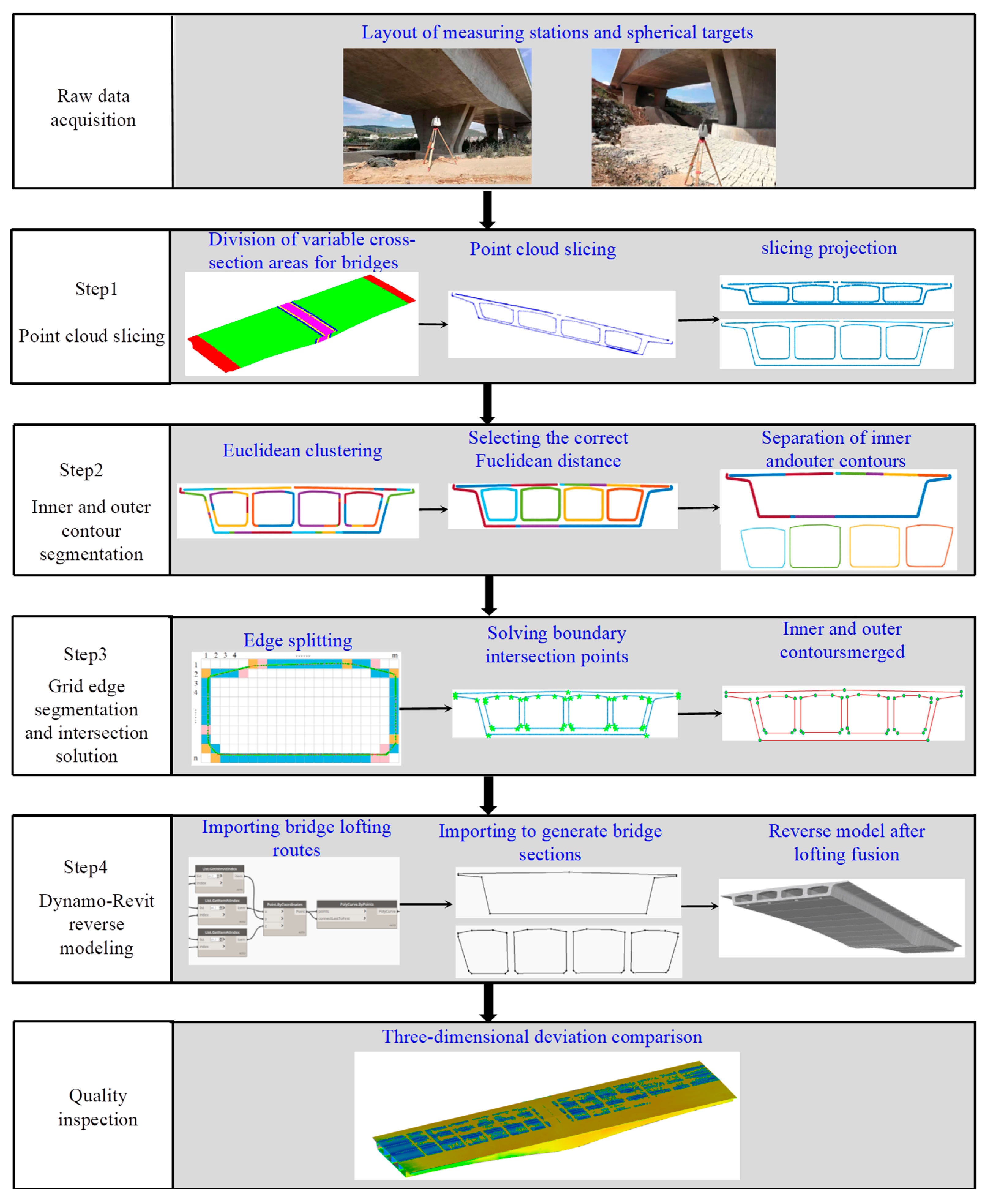
The composition of bridge structures is inherently more complex compared with those of building structures, making the generation of bridge gDT models a challenging task. Luo et al. [34] used the slicing method to extract point cloud features and used CATIA for reverse engineering based on these features, resulting in a modelling error of 8%. Wang et al. [35] proposed a fully automated detection and modelling method for MEP scenarios based on slicing, which enabled the modelling of a solid model for an indoor pipeline system. The cross-section types mainly consisted of circular and rectangular shapes, and the maximum average deviation between the model and the point cloud was 0.035 m. Zhao et al. [36] generated a reverse model by slicing the point cloud of prefabricated components and conducted quality inspection by comparing the reverse model with the design model. Tang et al. [37] utilised Revit and Recap to establish a 3D model based on point clouds and further employed the Revit family for parametric modelling. Zhou et al. [38] developed a BIM based on point cloud feature extraction for the virtual trial assembly of steel components. Qin et al. [39] used Dynamo–Revit to model single-box precast box beams, achieving a maximum deviation of 15 mm.

No single modelling software or platform can establish 3D models for all types of structures [40]. When dealing with complex components, information loss and subjective errors may occur due to human operations and other factors. However, the current modelling software and platforms available typically only offer standard components, such as pipes, walls, and rectangular beams [41]. The point cloud features extracted from the point cloud model provide fundamental parameters for reverse modelling [42,43,44,45]. In the context of 3D modelling based on point cloud data in housing construction, the focus is often on regular-shaped components, such as walls and roofs. For bridges, reverse modelling primarily concentrates on components with regular solid sections, such as piers, cap beams, T-beams, and other straightforward elements. In response to this situation, this paper adopts visual programming software Dynamo and Revit, employing a linked approach to effectively address the challenge of generating gDT models for bridges with complex cross-sections.

3. Method Framework

Figure 1 illustrates the principal steps of the proposed method outlined in this paper. The initial step involves planning the arrangement of targets and scanner stations, followed by the collection and pre-processing of bridge point clouds. Subsequently, four primary steps are involved in creating bridge gDT models, which include the extraction of point cloud features and the subsequent generation process:

Step 1: The first step involves longitudinal and horizontal slicing of the bridge point cloud. Euclidean clustering and grid segmentation algorithms are then applied to extract the coordinates of control points in the variable section segment. Subsequently, the bridge point cloud is divided into variable cross-section segments based on these control points, and the slices are projected into a 2D point cloud.

Step 2: In the second step, the 2D point cloud contour undergoes segmentation using the Euclidean clustering algorithm. This segmentation separates the inner and outer contours of the point cloud cross-section.

Step 3: The third step focuses on each contour individually, where segmentation and fitting are performed using a grid segmentation algorithm. This process results in obtaining the intersection points of adjacent edges for each contour.

Step 4: In the fourth step, Dynamo directly calls the Excel file containing the intersection coordinates of the cross-section. The bridge route and cross-section are generated using these coordinates, and the bridge gDT model is subsequently formed through cross-section lofting fusion.

Finally, to ensure accuracy, 3D deviation detection is performed between the bridge gDT model and the point cloud model.

4. Proposed Approach

This section proposes the bridge gDT generation method based on TLS. Section 4.1 describes the bridge point cloud acquisition method and point cloud registration method proposed in this study. The four steps in Figure 1 are introduced in Section 4.2 and Section 4.3. In addition, the DaDe Bridge in Section 5 is used as an example to verify the feasibility of the method proposed in this section.

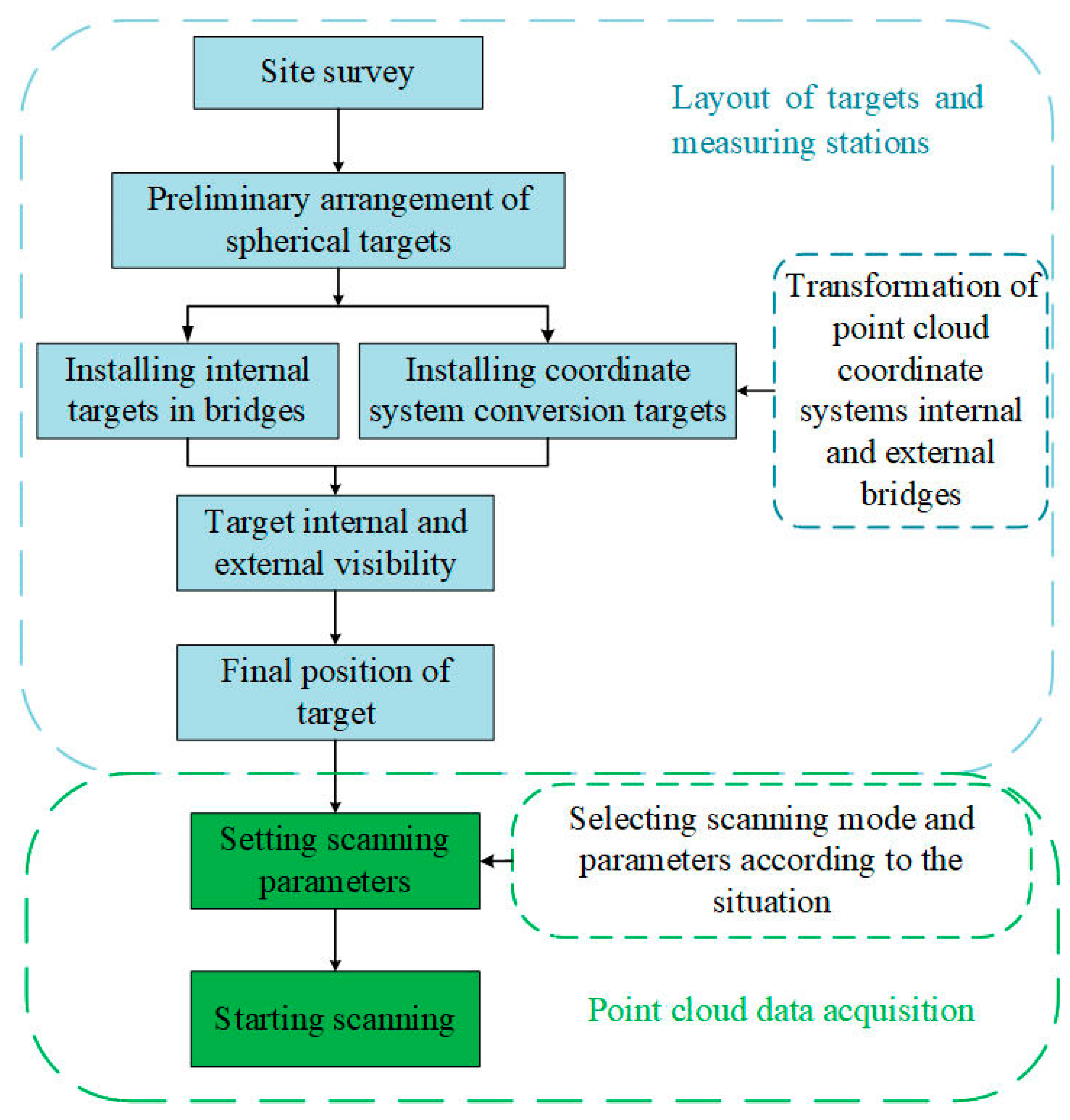
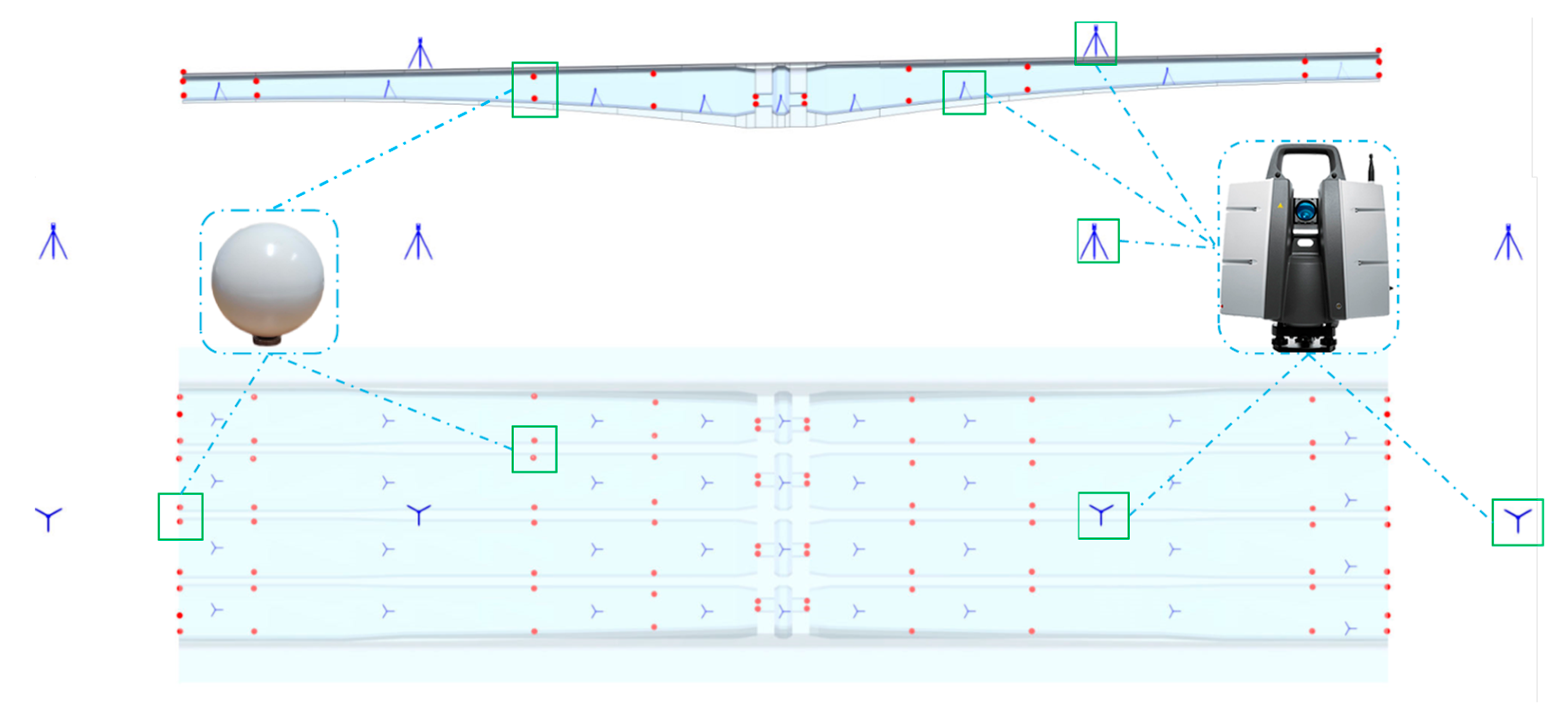
4.1. Point Cloud Acquisition Method

Due to the separation of the box and surface point clouds internal to the bridge, the two parts of the point cloud must be collected separately. The internal box chamber point cloud registration uses the target to register. Meanwhile, the external point cloud is registered using a two-stage approach that involves coarse and ICP fine registration. To ensure accurate point cloud registration, overlap between the point clouds of adjacent stations and points on the target for target fitting must be sufficient. Therefore, calculating the positions of the scanner station and target becomes necessary. The specific steps for collecting bridge point clouds are illustrated in Figure 2.

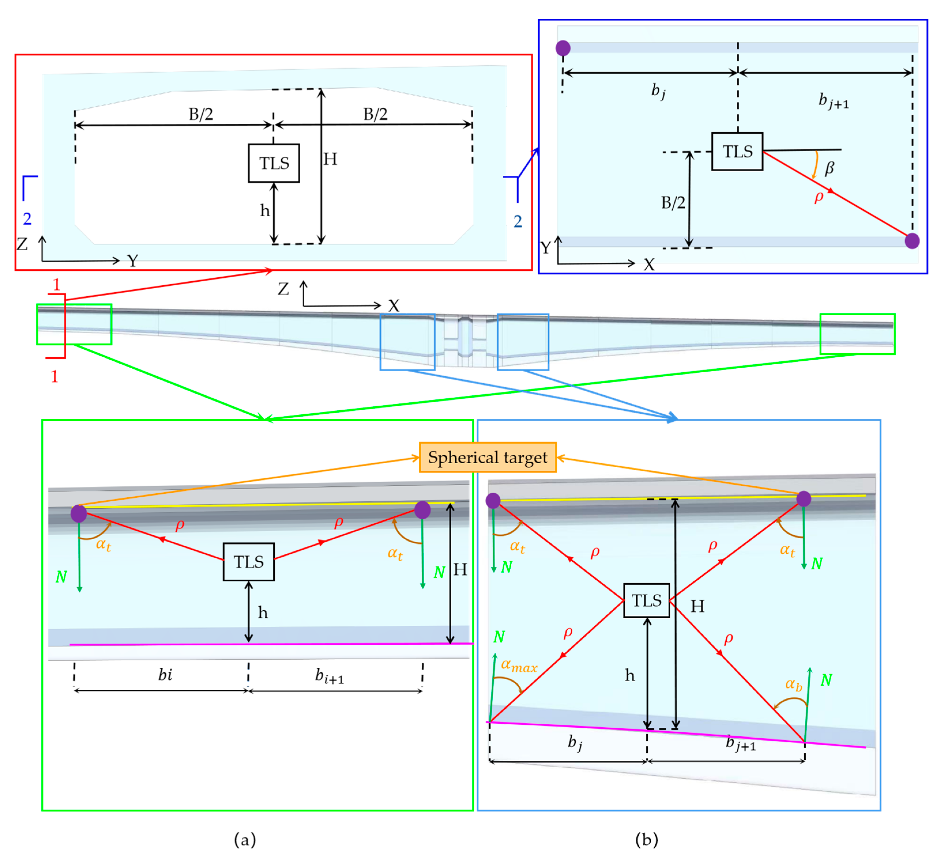
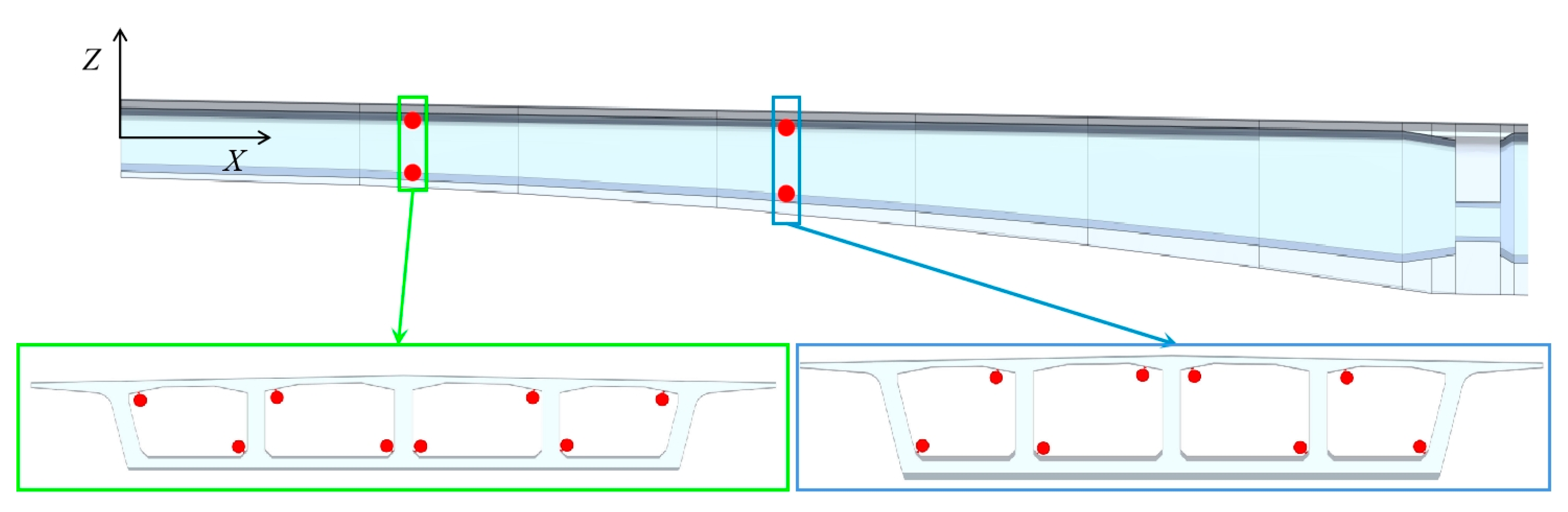
4.1.1. Layout Method of Internal Chamber Scanner Stations and Targets

In accordance with TLS principles, certain factors, such as incident angle, surface condition of concrete, and distance measurements, significantly influence the scanning process. Specifically, the internal box chamber of the bridge presents challenges because of its narrow scanning area, making it highly susceptible to the impact of incident angles and distance measurements. Incidence angles and ranging exceeding the threshold can lead to considerable noise, which subsequently affects the accuracy of point clouds. The relationship between the impact of incident angles and the distance from the sensor to the target on the received power is shown in Equation (1):

$$P_R\left(\rho \right)=P_T\frac{\cos \alpha }{{\rho }^2}\pi \gamma {\eta }_{sys}{\eta }_{atm}$$

(1)

where $P_T$ is the emission power, $\alpha$ is the incident laser line and the target plane normal, $\rho$ is the distance from the sensor to the target, $\gamma$ is the surface reflectance, ${\eta }_{sys}$ is the system losses, and ${\eta }_{atm}$ is the atmospheric losses.

During the scanning process inside the bridge box chamber, the surface condition remains relatively consistent. In this study, the parameter γ for the same bridge chamber is considered a constant. Additionally, the atmospheric transport effect is deemed negligible in TLS [46,47,48]. As a result, Equation (1) can be further simplified as follows:

$$P_R\left(\rho \right)=C\frac{\cos \alpha }{{\rho }^2}$$

(2)

where $C=P_T\pi \gamma {\eta }_{sys}$ is applicable for TLC scanning similar objects. As shown in Figure 3, the impact of incident angle and ranging on the received power is significant. The distance $b$ between the target ball and the scanner station directly influences $\alpha$. As b increases, $\alpha$ also increases, resulting in a decrease in received power and a decline in the quality of the obtained point cloud data. Due to the limited internal space of the box chamber, selecting a scanning mode with a smaller ranging and high resolution is advisable. The mode ensures the collection of point clouds with high point density and accuracy. For instance, for the Leica P50 3D scanner, the suggested scanning option is a range of 120 m, a resolution of 3.1 mm @ 10 m, and a single station scanning duration of 3 min. The distance between the 3D scanner and the target in the box is calculated with the incidence angle as the control threshold.

$b$ is calculated using the equation of changing the cross-section at the top of the bridge bottom plate and the greatest incidence angle. When $b$ is confirmed, $\propto$ meets the condition of ${\propto }_{max}>{\propto }_{t }>{\propto }_b$. Hence, ${\propto }_{max}$ will be utilised as the greatest incidence angle to calculate $b$. Finally, the distance between the instrument and the target in the box chamber is calculated using Equation (3) as follows:

$$\left\{\begin{array}{l}{b}_i=A\tan \left({\alpha }_{\max }\right)\cos (\beta ),A=\min \left[h,H-h\right]\hfill \\ b_j=\frac{y\left(x_{i-1}\right)\left(h+y_{i-1}\right)-\tan \left({\alpha }_{\max }\right)\left(y_{i-1}-h\right)+2x_{i-1}+1}{\tan \left({\alpha }_{\max }\right)y^{\prime }\left(x_{i-1}\right)-1}\cos (\beta )\hfill \end{array}\right.$$

(3)

where $b_i$ is the distance between the target and the measuring station in the constant beam height section; $b_j$ is the distance between the target and the measuring station in the variable beam height section; A is the smaller value of the difference between the height of the box; H is the height of the box chamber; h is the instrument height; y is the longitudinal variable cross-section equation of the box beam bottom plate; $\beta =\arctan \left(B/2b\right)$ is the angle between the centerline of the compartment and the line connecting TLS and the target ball; B is the width of the box chamber; and ${\mathrm{x}}_{\mathrm{i}-1}$ is the x-coordinate of the previous target in the measuring station; $\mathrm{y}\prime$ is the first derivative of y at x.

At least two targets are positioned within each target layout section, and they are placed at the corners of the cavity. The cross-sections of adjacent targets are arranged, as depicted in Figure 4.

4.1.2. Layout Method of External Scanner Stations for Bridges

The collection of external point clouds for bridges is divided into two parts: point cloud collection of the bridge deck and point cloud collection of the bridge bottom. When arranging stations for bridge deck point clouds, the impact of the incident angle on the accuracy of the point cloud must be considered. The calculation principle of the distance between two neighbouring scanner stations is shown in Figure 5. The distance $b_i$ is calculated using Equation (4).

$$b_i=2h\tan ({\alpha }_{\max })$$

(4)

The collection of point clouds below the bridge necessitates scanning both sides and ends of the bridge. When scanning at the bottom of the bridge, the incident angle is relatively small, and the impact of the incident angle can be disregarded.

4.1.3. Registration Method for External and Internal Point Clouds of Bridge

Box Chambers

Bridge point clouds are registered according to the process presented in Figure 6. This process can be divided into five main parts: registration of the bottom point cloud, registration of the deck point cloud, registration of the bottom point cloud to the deck point cloud, registration of the interior chamber point cloud, and overall registration of the surface and box chamber point clouds. The bottom and deck point clouds are registered using a two-stage method comprising coarse registration and ICP accurate registration. Additionally, the point cloud within the bridge cavity is registered utilising targets. However, due to limited visibility between the box chamber and the bridge exterior, the common overlap between the two parts of the point clouds is relatively small, which does not meet the conditions required for ICP registration.

Therefore, this study proposes a method of installing targets at the manhole to establish a unified coordinate system for the external and internal parts of the bridge. Although the manhole provides favourable sight conditions for both inside and outside the bridge, the sight range is limited and may not meet the conditions required for ICP registration. To address this, the registration of point clouds inside and outside the bridge is achieved by placing spherical targets at each manhole. To ensure registration accuracy, two targets should be arranged at each manhole. These targets are placed in opposite directions at the manhole, with their target base diameter coinciding with the upper edge of the manhole, as shown in Figure 7c,d. Additionally, the TLS at the manhole is arranged following Figure 7a,b and positioned at the centre of each maintenance entrance, perpendicular to the ground. The measurement station is located near the manhole inside the box chamber.

4.2. Method for Extracting Bridge Section Features

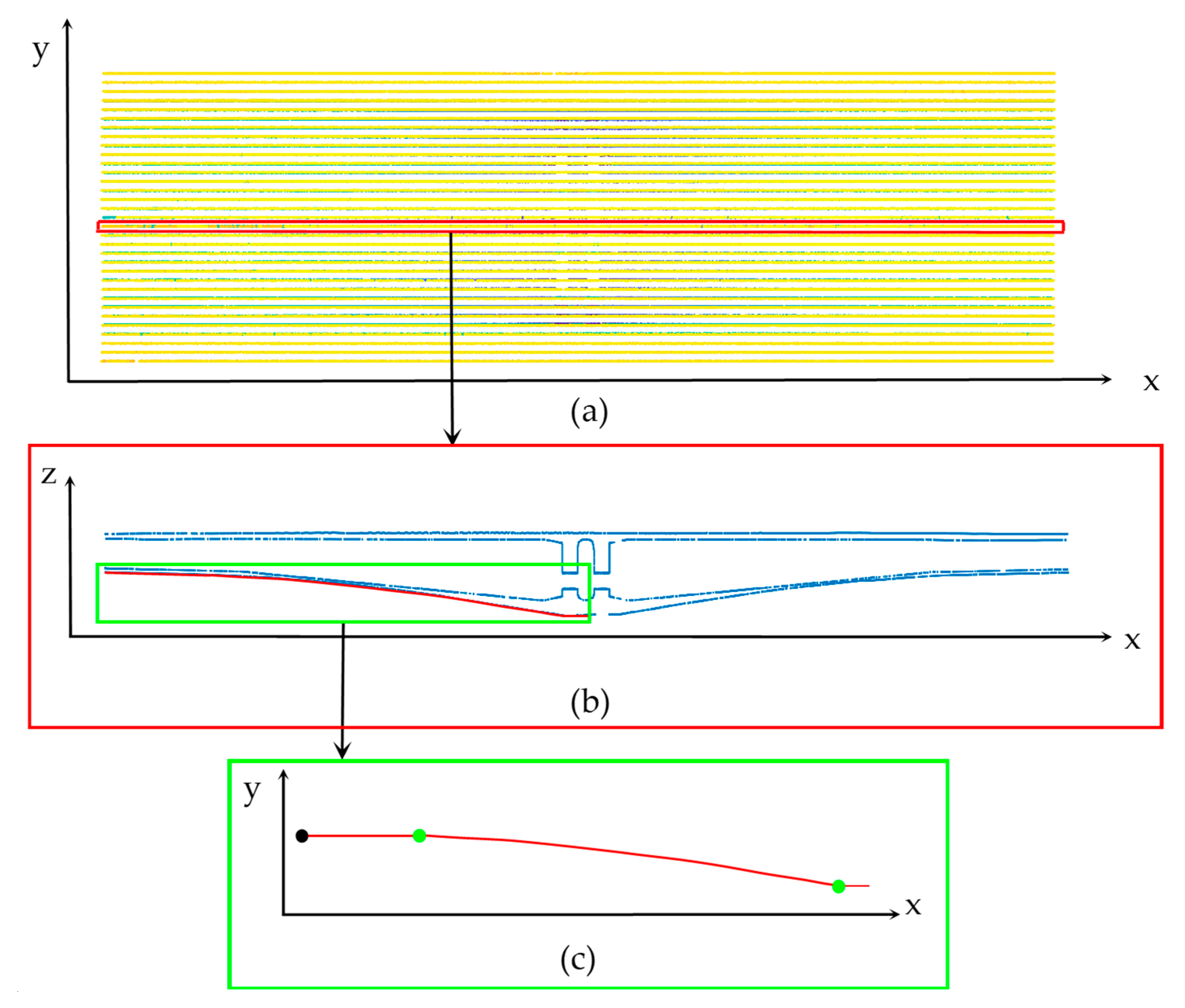
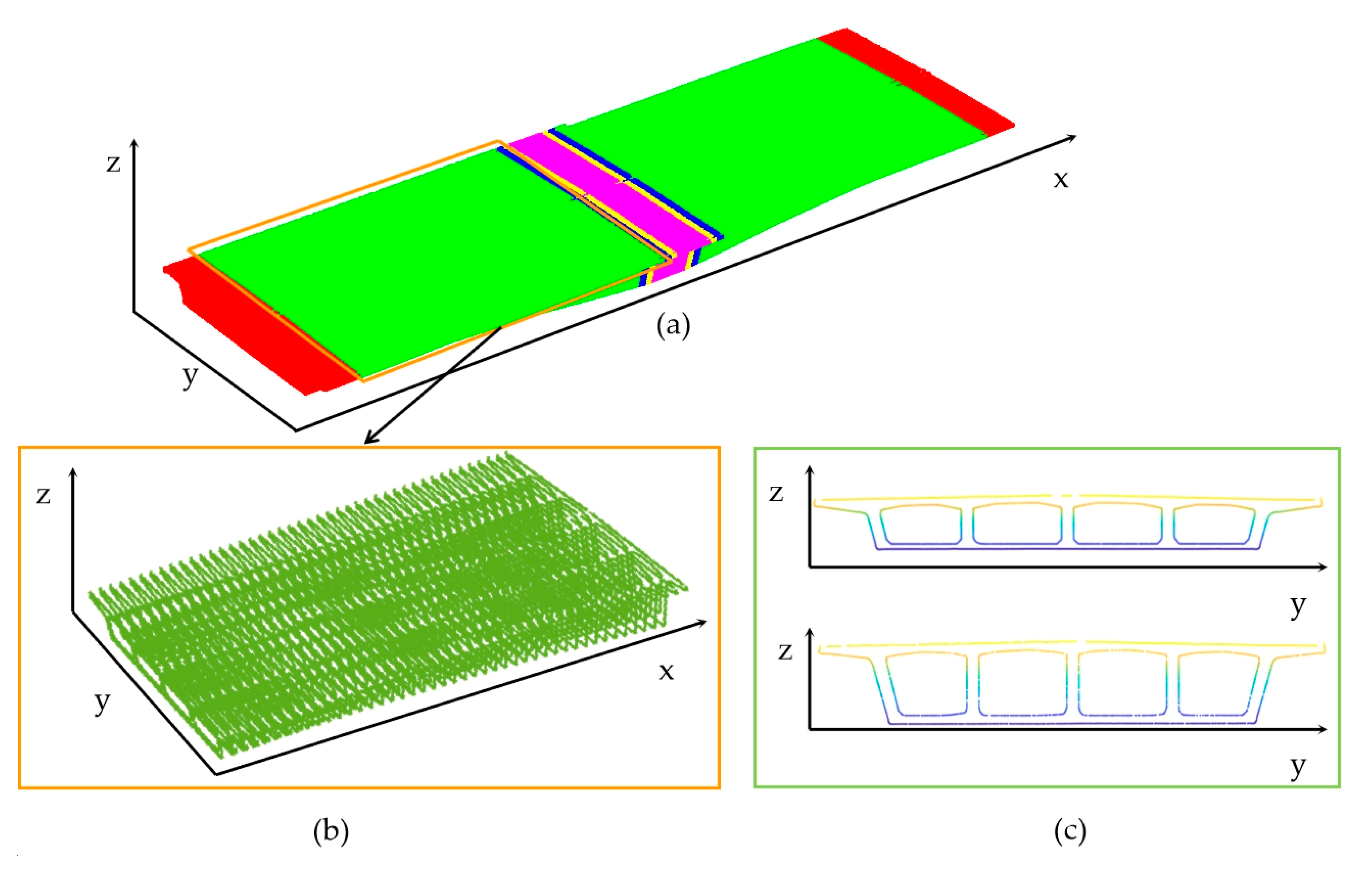
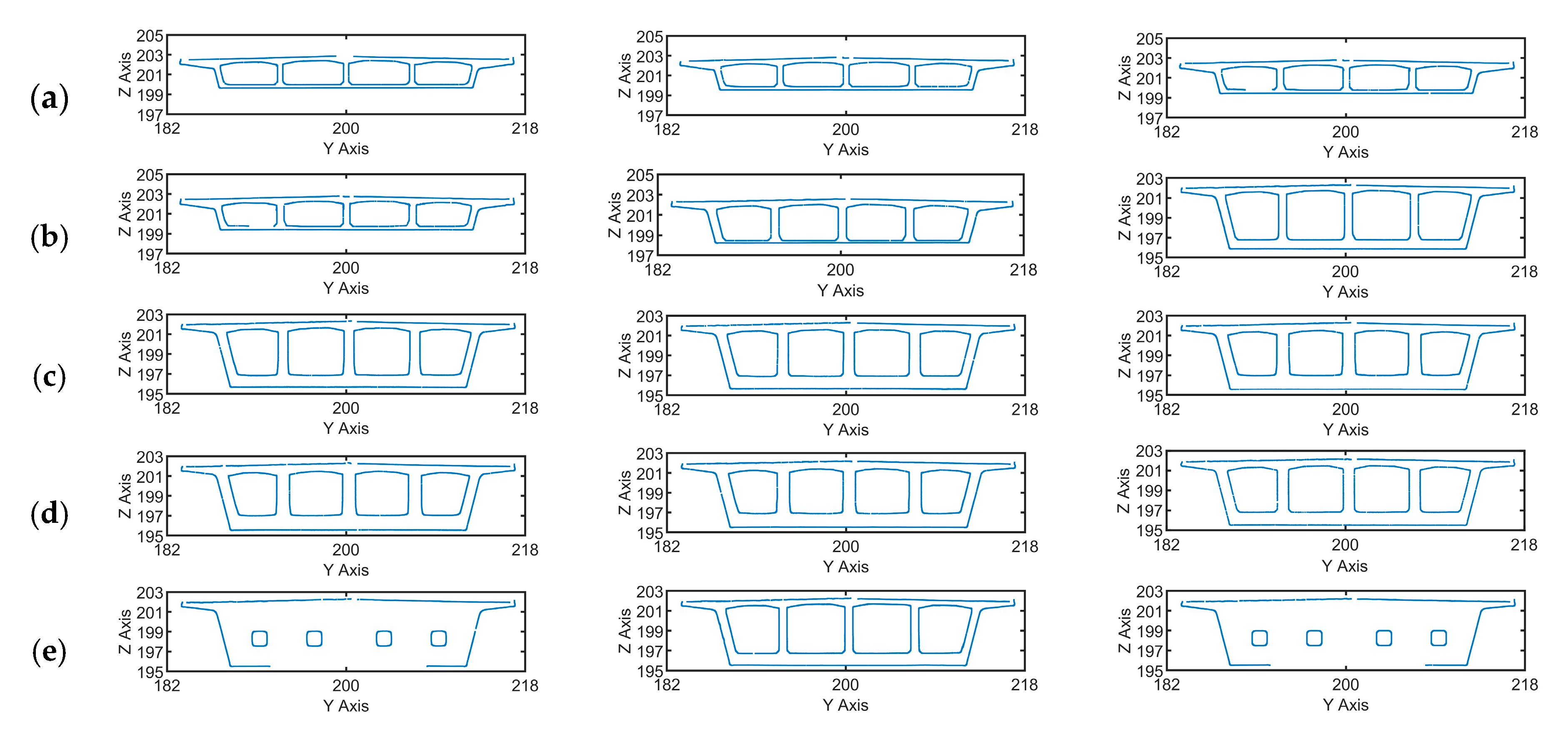
4.2.1. Point Cloud Slicing of Bridge

The reverse modelling of the starting and ending points of the variable section of a bridge holds particular significance. To determine the control section position of the variable section, clustering and grid segmentation algorithms are proposed to extract the control section position. The variable section of the bridge consists of two parts: the internal web plate variation section and the external beam height variation section. Therefore, the method separately extracts the coordinates of the starting and ending points of these two variable segments. Afterwards, the extracted coordinates are sorted in ascending order based on their x-coordinate values. Ultimately, the bridge is divided into different variable cross-section segments based on the x value of the coordinates.

The method mainly consists of three steps. Firstly, the pre-processed point cloud model is rotated so that the longitudinal and transverse directions of the bridge are aligned with the x and y axes, respectively. Secondly, the extraction of control section coordinates is divided into two main parts.

Part 1: The coordinate extraction of the web variable section is divided into four steps: (1) The bridge is sliced vertically along the z-axis, as shown in Figure 8a. (2) The Euclidean clustering method is used to separate the box chamber contours from the slice point cloud, as illustrated in Figure 8b. (3) The contour of the 1/2 width box chamber is segmented using Section 4.2 grid segmentation algorithm for edge lines, and the segmented point cloud edge lines are fitted, as seen in Figure 8c,d. (4) The solved lines are sorted by slope, and the intersection points of adjacent edge lines are determined. The black point in Figure 8d serves as the starting point of the variable cross-section segment, taking the intersection point between the solid section edge line of the bridge and the web edge line. Consequently, the coordinates of the control section inside the box chamber can be obtained.

Part 2: The coordinates of the control section for the beam height variation section are extracted in four steps: (1) The bridges are sliced vertically along the y-axis, as shown in Figure 9a. (2) The lower edge line of the bridge bottom plate is extracted using the Euclidean clustering algorithm, as depicted in Figure 9b. (3) The Euclidean clustering algorithm is used to segment the bottom edge of the beam. Then, the segmented beam bottom edge is further segmented and fitted using a clustering algorithm based on curvature. (4) The fitted point cloud edges are sorted according to curvature, and the intersection points between adjacent edges are determined, as shown in Figure 9c.

Finally, the bridge is divided based on the extracted coordinates of the control sections, as illustrated in Figure 10a. After dividing the variable cross-section section, it is sliced along the longitudinal bridge direction. During this process, the projected thickness $\mathsf{\Delta }$ plays a crucial role in point cloud feature extraction.

The calculation of the average density $\rho$ of point clouds is performed to determine the projected thickness $\mathsf{\Delta }$ of point cloud slices. Points $F_1,F_2,F_3\dots \dots ,\mathrm{and} F_b$ are randomly selected points from the point cloud as query objects, with each query object as the centre and $R$, the radius of the circle, as the range threshold. If the number of points within the query range is $P_i$, then the value should satisfy Equation (5).

$$\left\{\begin{array}{l}\rho =\frac{{\displaystyle \sum \left[P_{Fi}/\left(\pi R^2\right)\right]}}{b},i\in \left(i,b\right)\hfill \\ \Delta =k\rho ,k\in [2,4]\hfill \end{array}\right.$$

(5)

The larger the empirical parameter $k$ value, the more complete the features are maintained, and $\mathsf{\Delta }$ increases accordingly. However, a larger $\mathsf{\Delta }$ can lead to redundant points in the projection cross-section, potentially reducing the reliability and accuracy of the projected point cloud edges. Thus, selecting an appropriate k value based on the actual characteristics of the point cloud is crucial. For different variable cross-section segments, corresponding slice spacing is used for point cloud slicing. Figure 10b illustrates the point cloud slice of the variable section segment, and Figure 10c shows the contour of the point cloud after projection.

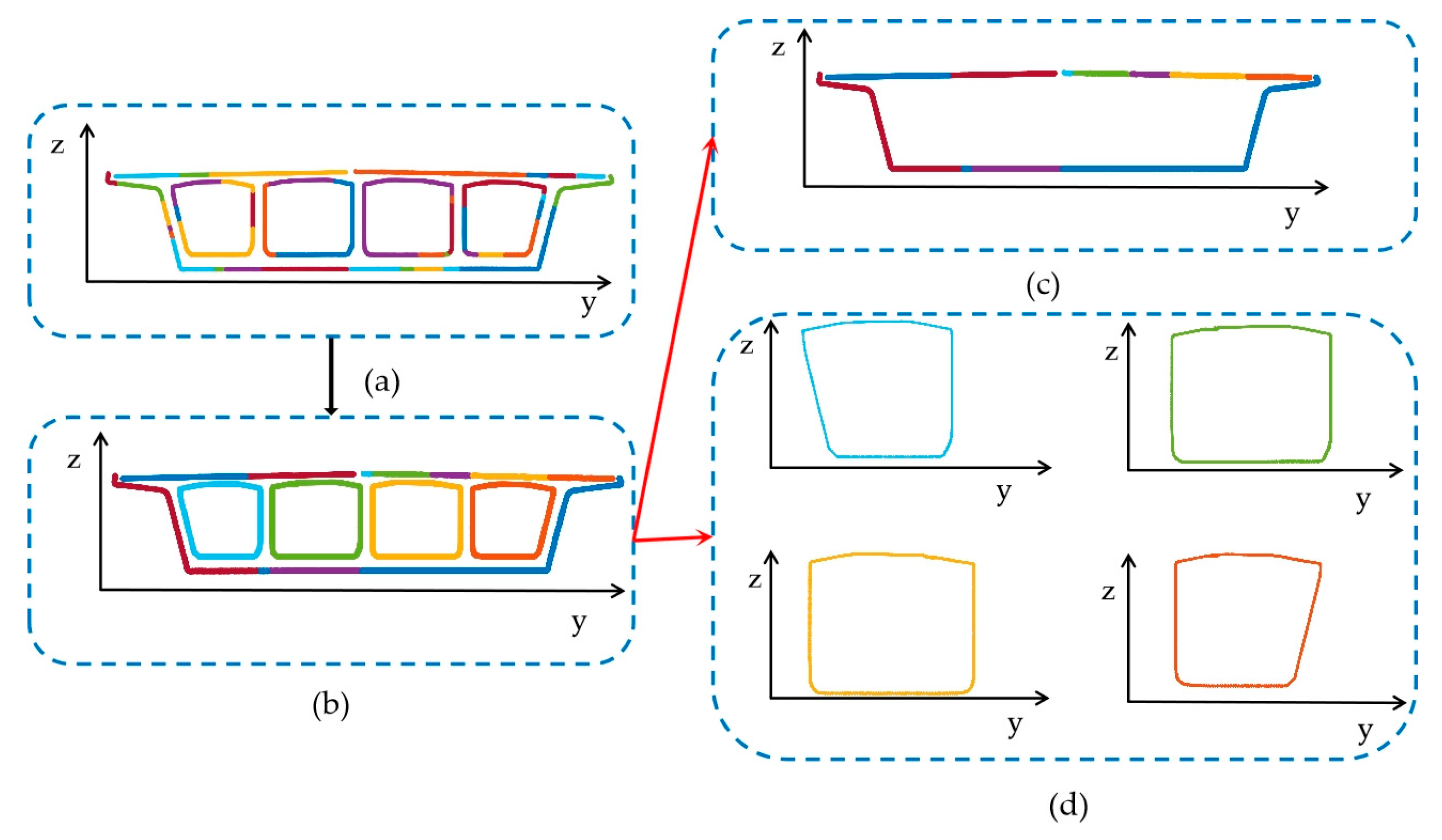
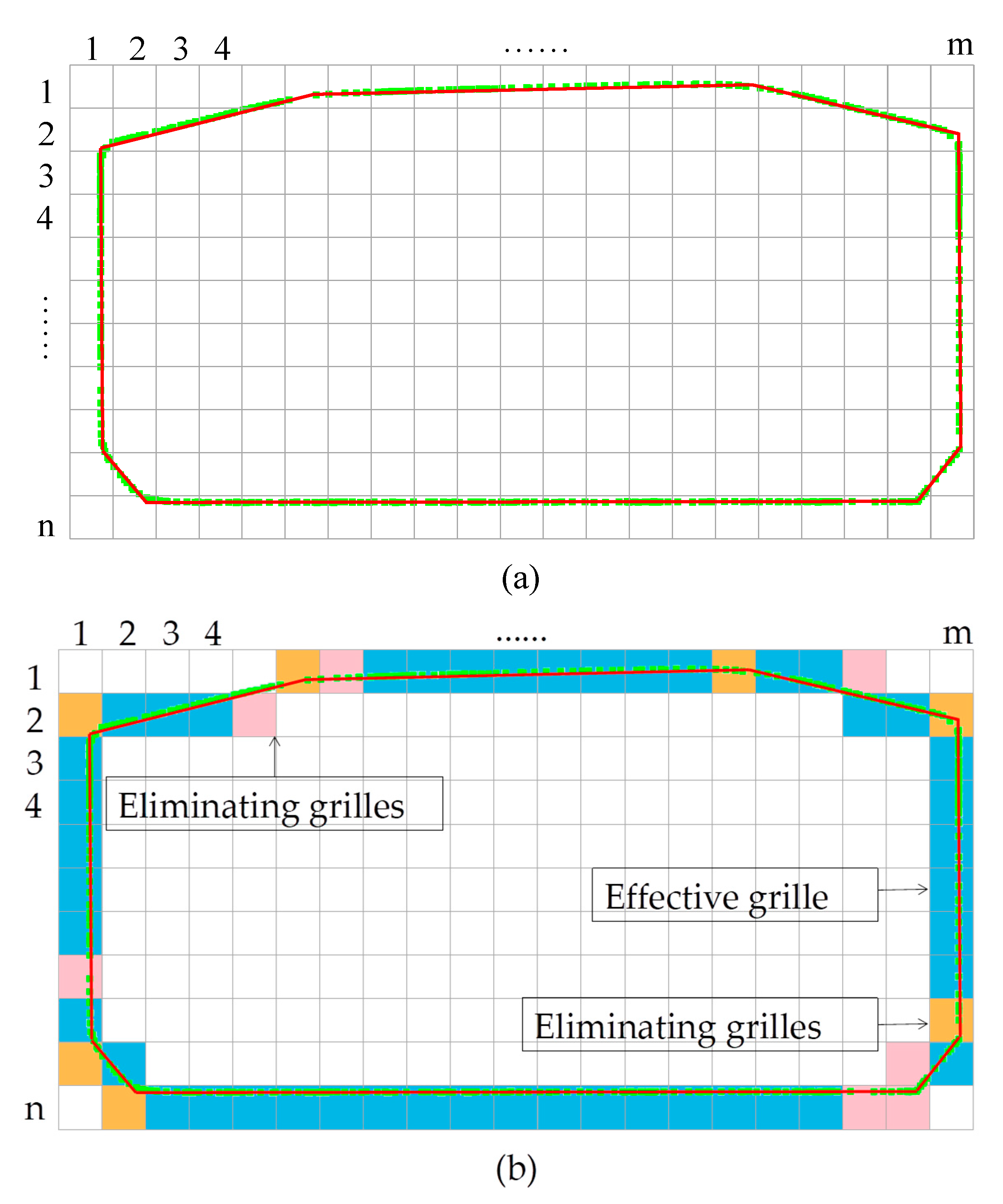
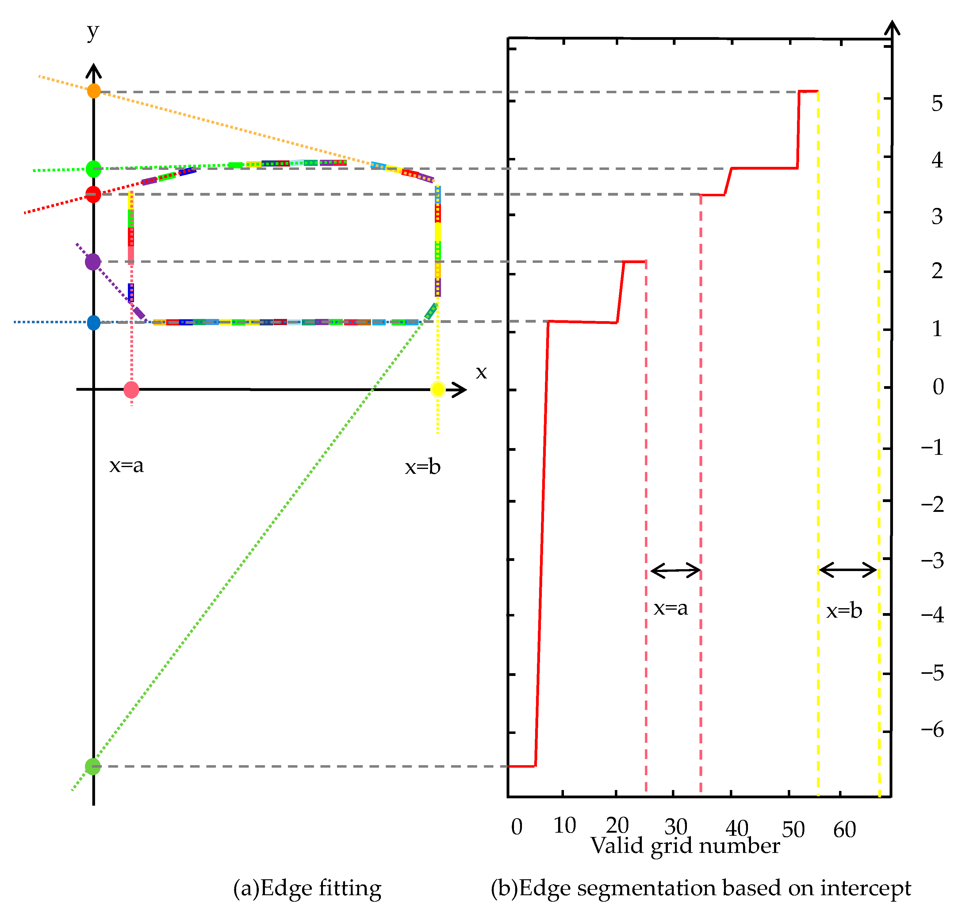
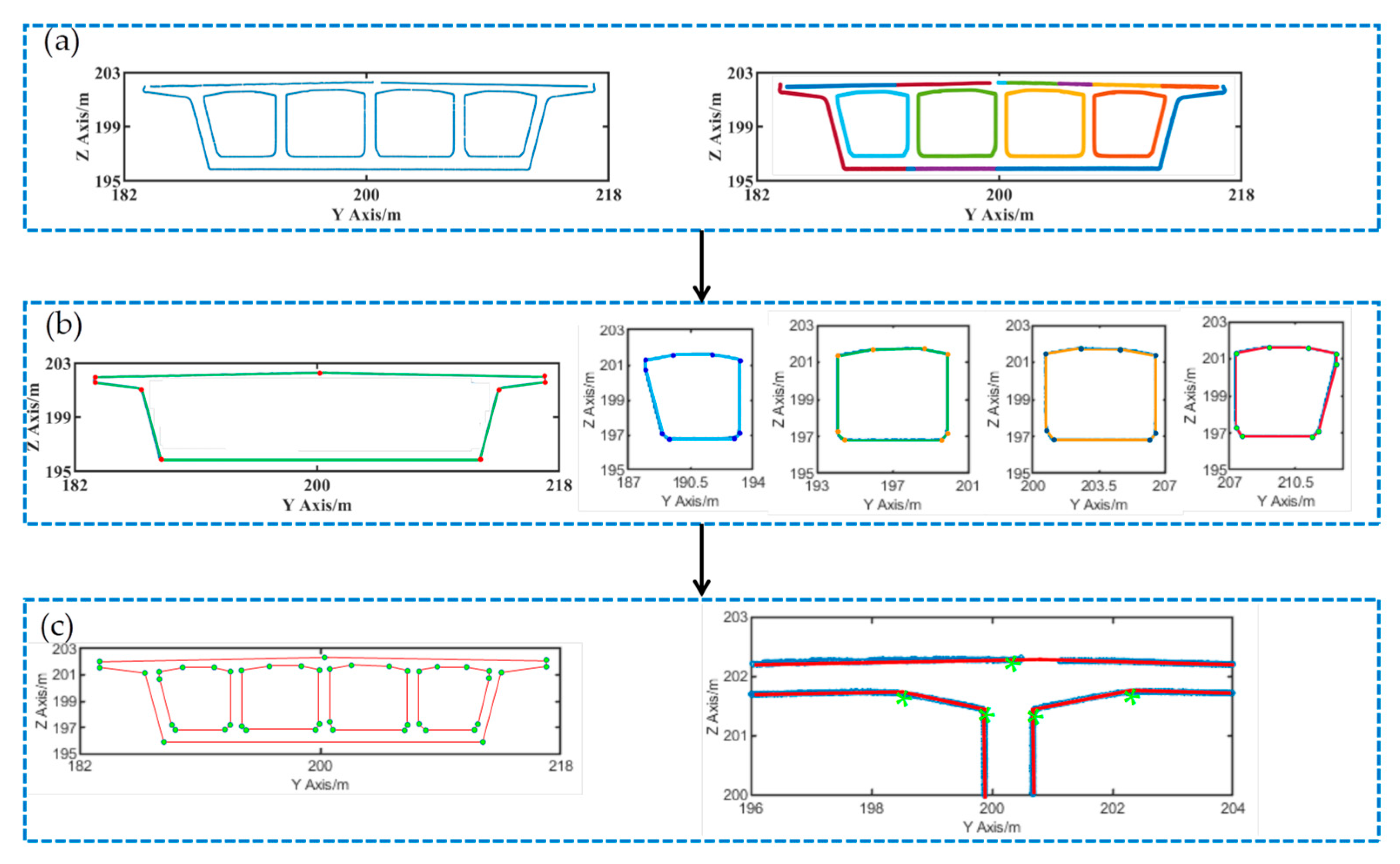
4.2.2. Point Cloud Feature Extraction

The feature extraction based on slice point clouds mainly consists of two steps:

Step 1: The projected slice point cloud uses a clustering algorithm to segment the inner and outer contours of the cross-section. The query point $F_i$ is randomly selected from the point cloud contour. By calculating the Euclidean distance $l_j$ between $F_i$ and the adjacent point $K_j$, the minimum Euclidean distance $L_{min}$ between $l_j$ and different cluster points is compared. When $l_j$ is greater than $L_{min}$, $F_i$ and $K_j$ belong to the same cluster point group. When $l_j$ is less than $L_{min}$, they belong to a different cluster point group. When the conditions of Equation (6) are met, the Euclidean clustering method can accurately separate the inner and outer contours of the point cloud, as shown in Figure 11.

$$m\rho \le L_{\min }\le d_{\min }$$

(6)

where $d_{min}$ is the minimum distance between the inner and outer contours of the bridge, and m is the empirical parameters.

Step 2: A grid method is proposed for the feature extraction of contours. The first step in using the grid segmentation algorithm is to determine the grid size, d; the number of points in the grid, p; and the standard deviation, q, of the point cloud fitting line within the grid. d and p are related to the point spacing of the point cloud cross-section. The parameters are assigned values by analysing the contour of each segmented point cloud. Subsequently, the 2D point cloud is assigned to the grid, as depicted in Figure 12a. The grids containing point clouds are filtered based on the number of points within the grid and the standard deviation of the point cloud fitting line, as shown in Figure 12b. Blank grids, grids with fewer points, and grids with corners are filtered out, retaining the effective grids. The remaining point clouds within the grids are linearly fitted separately. Considering that parallel edges are observed in the cross-sectional contour line, using the slope for classification is not feasible. Therefore, for edges with a straight line slope, each grid obtained is linearly fitted, and the lines are classified based on the slope. The point clouds within the grid are divided into a set of points with a similar intercept, and the points within this set are linearly fitted to obtain the line equation of this boundary line. For edges without slope, the y-axis of the boundary line does not intersect, so the intercept on the y-axis cannot be obtained. However, these edges without slope have distinct geometric features, and their linear equations can be directly obtained, as illustrated in the two straight lines x = a and x = b in Figure 13. Finally, the fitted edges are solved for contour intersections in grid order. The specific steps of the grid segmentation algorithm are presented in Algorithm 1.

Algorithm 1: grid segmentation algorithm

Input: Section point cloud Datan×2; //Convert to a section point cloud on a 2D coordinate system. Output: Crosspoint 1. For i = 1:n do 2. j = x_Data(i)/d, k = y_Data(i)/d; //Calculate the coordinates of the i-th row in the grid in Data, d is the grid size. 3. Box{j, k} = Data(i); //Traverse all points in the Data and assign them to the corresponding grid. 4. End For 5. If length(Box{j, k}) > p or std(error_linefit(Box{j, k})) < q; //P is the screening condition for the number of points in the grid, and q is the screening condition for the standard deviation of line fitting residuals. 6. Box_good{m} = Box{j, k}; //Box_ Good is the effective grid point cloud stack, and the initial value of m is 1. 7. [a(m) b(m)] = linefit(Box{j, k}); //a is the slope of the grid fitting line, and b is the intercept of the grid fitting line. 8. m = m + 1; 9. End If 10. [b1 b2 b3 …br…] = Sort b; //Obtain the approximate intercept b1, b2, b3 …br… of the edge fitting line through sorting and clustering. 11. Pointcloud(r) = Box_good{find(b==br)}; //By determining whether the intercept b of any grid is merged with the approximate intercept br of the edge line, it belongs to a certain edge line grid point cloud. 12. Line(r) = Linefit(Pointcloud(r); //Accurately calculate the fitting line for each edge line. 13. Crosspoint(r) = Solve(Line(r) Line(r + 1)); //Solve the intersection points of adjacent lines in grid order. 14. End

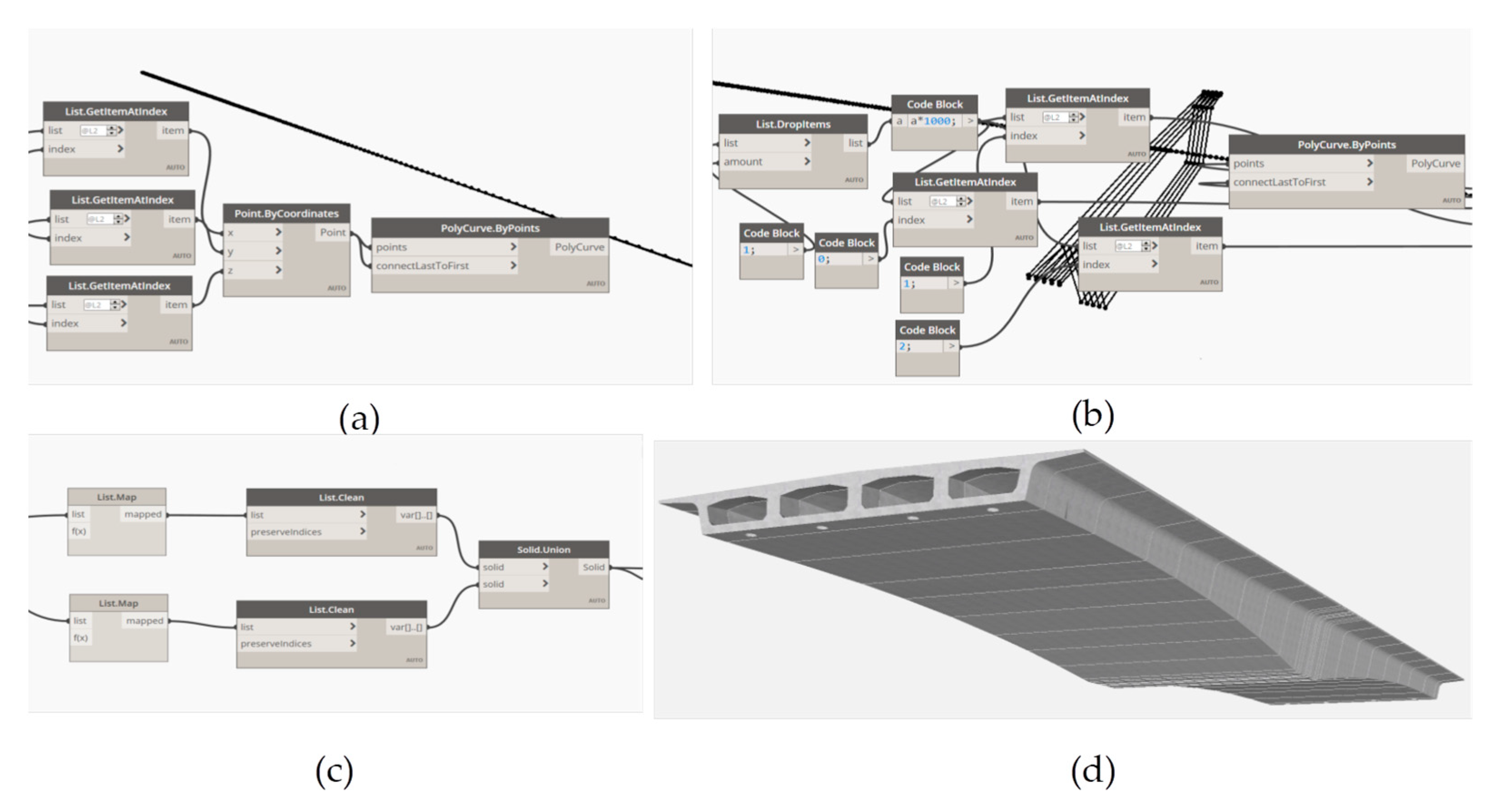
4.3. Dynamo-Revit Reverse Modelling Framework

The intersection coordinates extracted from the point cloud model are exported to an Excel file. The Dynamo platform is utilised to access the Excel file automatically, enabling the automatic generation of the bridge gDT model based on point cloud feature extraction. The gDT model generation process can be divided into three main steps:

Step 1: Dynamo automatically retrieves the coordinates of the bridge route. After extracting section features, select the point with the highest Z coordinate value for each section as the base point of the section. The base points of all sections are arranged from small to large according to the X coordinate value, connecting the base points to form the bridge route. The polycurve.bypoints node is then used to automatically connect each coordinate point to form the bridge route, as depicted in Figure 14a.

Step 2: Considering the section coordinate data provided by this method represent the actual bridge section coordinates, the coordinate system does not need to be converted. Dynamo automatically retrieves the coordinates of the intersection points of the profiles of each section of the bridge from Excel. The Polygon.bypoints node is used to generate the outer and inner profiles of the bridge section, respectively, as shown in Figure 14b.

Step 3: The generated contours are lofted and fused using the Solid.byloft and List.map nodes along the route for the outer and inner contours. Subsequently, the Solid.Difference node is employed for Boolean operations to generate the bridge gDT model, as illustrated in Figure 14c,d.

5. Experiment

To verify the feasibility of the proposed method in this study, a single box and four-chamber concrete bridge are modelled through scanning. The experimental details are presented in Section 5.1, while the experimental results are summarised and discussed in Section 5.2.

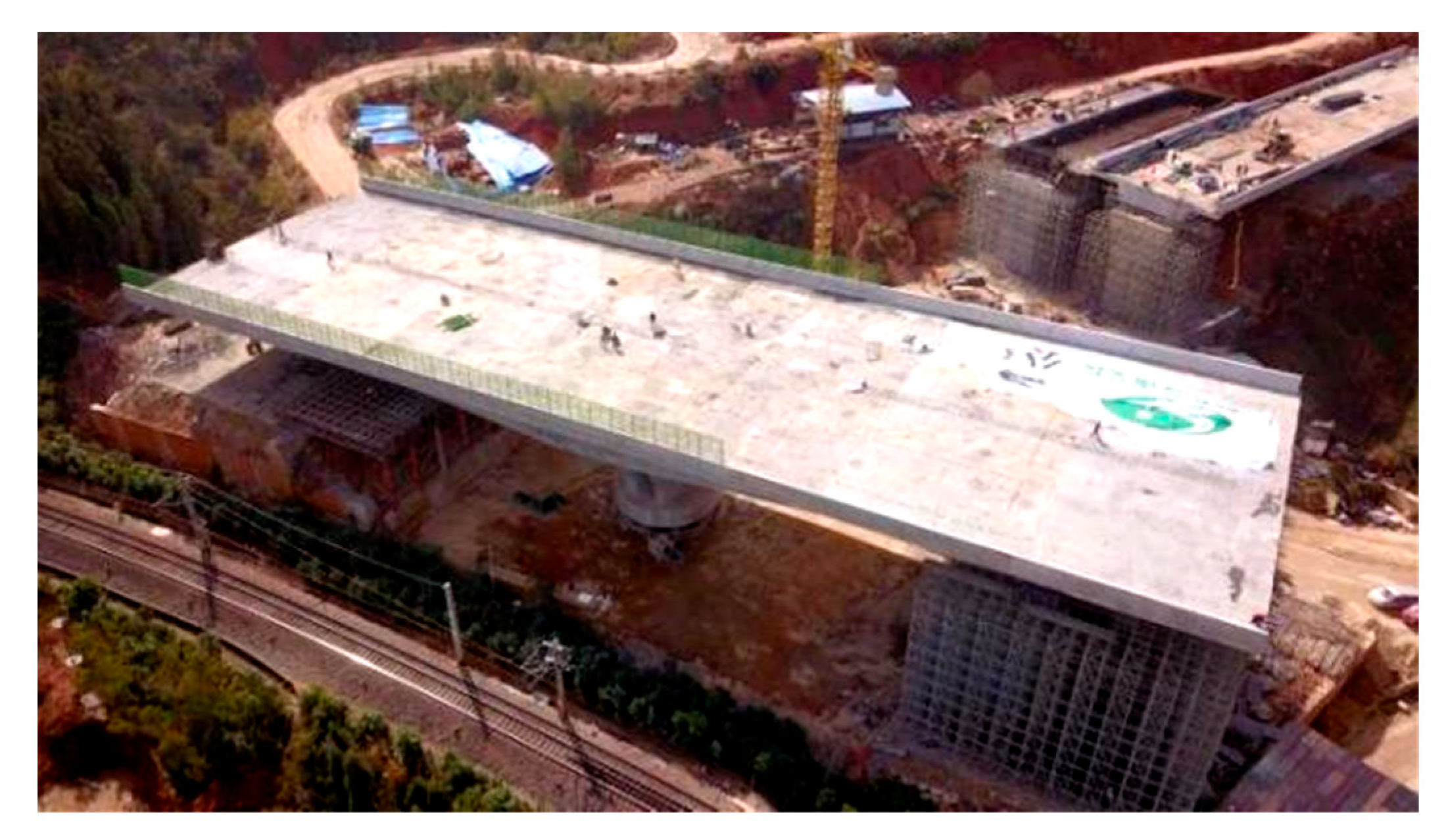
5.1. Experimental Information

The bridge is situated over the Chengdu-Kunming railway. To ensure the operational safety of the existing railway lines during the bridge construction, a horizontal rotation method is employed. The construction team is required to complete the bridge rotation within a short timeframe. This bridge is characterised by its substantial weight, with a theoretical self-weight of approximately 1.5 × 10⁴ tons, making it the second-largest tonnage swivel bridge in Yunnan Province. It has a total length of 290 m, which includes a main bridge with a swivel section that spans 121 m and a bridge deck width of 33.5 m. The bridge’s minimum beam height is 3 m, and the maximum beam height is 6.5 m. Moreover, the minimum cavity height is 2.45 m, and the maximum cavity height is 5.05 m. The rigid frame bridge rotates counterclockwise by 66° to reach its completed position, as depicted in Figure 15.

The scanner utilised in this study is the Leica P50, with a scanning mode of 120 m ranging and a resolution of 3.1 mm @ 10 m. Following the target and station layout method proposed in Section 4.1, the bridge deck measurement stations are arranged as two stations on each side along the bridge and one station at each end of the bridge, resulting in a total of eight external scanner stations for the bridge. Additionally, there are 36 internal box chamber scanner stations, making a total of 44 scanner stations for the entire bridge. The layout of stations and spherical targets can be seen in Figure 16. The time loss of bridge scanning mainly includes calculating the position of measuring stations and targets, arranging spherical targets and scanners, and moving scanners. The time required for calculating the station and target positions is 10 min, the scanner working time and target and station layout time of each scanner station is 6 min, and the movement of the entire bridge measurement station lasts 86 min. The total time required for full bridge scanning is 360 min. The total number of point clouds captured for the entire bridge amounts to 5.86 million. Notably, a prism does not need to be set up, making the process more efficient than using Total Station to measure the geometric parameters of bridges.

The raw point cloud presented in Figure 17 exhibits a noticeable initial attitude error. To rectify this, the bridge deck point cloud and the bridge bottom point cloud are registered using the Iterative Closest Point (ICP) method, with the mean square error of the iteration set to ${\epsilon }_{min}=0.001$. Following this, the box chamber point cloud and surface point cloud are registered through the use of spherical targets, resulting in a maximum registration error of 2 mm for the entire bridge. Figure 18 displays the registered point cloud. An analysis of the full bridge point cloud and local point cloud indicates that the point cloud registration accuracy is reliable, with no point cloud layering phenomenon observed, and subsequent system errors have been minimised.

The bridge point cloud is manually segmented from the point cloud model. The pre-processed point cloud model utilises the point cloud slicing method described in Section 4.2. As the bridge comprises multiple variable sections, the variable section division method from Section 4.1 is applied to divide the bridge into 9 variable sections. The left and right sides of the bridge are symmetric with respect to the centreline of the bridge pier. The distribution of the left half-span slice areas is as follows: the first region has a length of 7.5 m, and the slice spacing is 50 cm; the second region has a length of 48.4 m and a slice spacing of 40 cm; the third region has a length of 1.1 m and a slice spacing of 10 cm; the fourth region has a length of 0.9 m and a slice spacing of 30 cm; and the fifth region has a length of 5.2 m and a slice spacing of 10 cm. The thickness of the projection slice is 8 cm, and the division of the right and left variable cross-section segments is identical. In total, the entire bridge is divided into 352 slices, with some of them displayed in Figure 19.

According to the analysis of point cloud slice contours, some missing edges in the point cloud contours are observed, but it does not affect the extraction of point cloud cross-sectional features. The Euclidean clustering algorithm is utilised to separate the inner and outer contours of the point cloud cross-section after slicing and projecting. Considering the minimum top plate thickness of the bridge to be 25 cm and the minimum bottom plate thickness as 30 cm, we set $L_{min}=24 \mathrm{cm}$. As a result, the cross-section is divided into one outer contour and four inner contours, as depicted in Figure 20b. The segmented contour is fitted to the boundary equation using a grid segmentation algorithm, and the intersection points of the lines are calculated. Finally, the five profiles are assembled to obtain the box girder cross-section, as illustrated in Figure 20c.

Finally, Dynamo calls the intersection feature parameters of each section to generate the route and cross-section of the bridge. The contours and routes generated by Dynamo are fused through extruding and Boolean operations to generate a bridge gDT model, as shown in Figure 21.

5.2. Result

Firstly, the locations of scanner stations and targets are calculated using the method proposed in Section 4.1, with 44 stations and 84 targets arranged throughout the bridge. Then, 352 slice point cloud features are successfully extracted using the methods proposed in Section 4.2. According to Section 4.3, the bridge gDT model is successfully generated using the proposed framework. Finally, the gDT model is exported to IFC format through Revit, and the IFC file is imported into Geomagic for 3D deviation comparison with the raw point model. Figure 22 shows the comparison results of 3D deviations, with a uniform distribution of deviations. The maximum deviation is 6.6 mm, and the average accuracy is within 3 mm, indicating that the generated gDT model closely aligns with the point cloud data.

5.3. Discussion

During the gDT model generation process, there are several aspects we should pay attention to. On the one hand, the minimum Euclidean distance $L_{min}$ has a significant effect on the separation of the inner and outer contours of the slice in Section 4.2.1. In this bridge, the minimum distance between the inner and outer contours of the swivel bridge is 25 cm. To analyse the contour segmentation effect under different values of $L_{min}$, the slices are segmented from 10 cm to 25 cm in steps of 1 cm. According to Figure 23, when $L_{min}$ satisfies the condition of $L_{min}\in \left[22,24\right]$, it can accurately segment the inner and outer contours of the point cloud slice. If $L_{min}$ is less than 22 cm, then the phenomenon of missing mages in segmenting contours is caused by missing point clouds. If $L_{min}$ is more than 25 cm, then the phenomenon of missing edges in segmenting contours is due to point cloud drifting and surface defects on the enclosure. On the other hand, in the process of extracting point cloud features through grid segmentation, the standard deviation q of point cloud fitting lines within the grid directly affects the accuracy of edge fitting and the number of grids. If the value of q is less than the appropriate range, then it will result in a decrease in the number of points for final edge fitting and the loss of short edges. If the value of q is greater than the appropriate range, then it will cause a decrease in the accuracy of edge fitting. Therefore, this paper suggests that the value of q should be in the range of [0.004, 0.006], which can ensure the integrity of the edges and have high fitting accuracy. However, some positions still have deviations between the gDT model and point cloud, mainly due to the following reasons: (1) errors being generated by point cloud registration; (2) the error caused by multiple format transformations of the bridge gDT model; and (3) system errors caused by point cloud slice projection and feature extraction algorithm calculations during the point cloud feature extraction process. Despite these deviations, the results indicate the feasibility and accuracy of the proposed method in this paper.

6. Conclusions

This study proposes a method for gDT twin models of RC bridges with box chambers based on TLS. The main contributions of this study are summarised as follows: (1) this paper introduces a rapid data collection method for point cloud data in bridges with box chambers; (2) an automatic extraction algorithm for bridge section features based on Euclidean clustering and grid slicing of point clouds is proposed; and (3) a framework for automatic generation of bridge gDT models based on Dynamo-Revit is established. The specific conclusions are as follows:

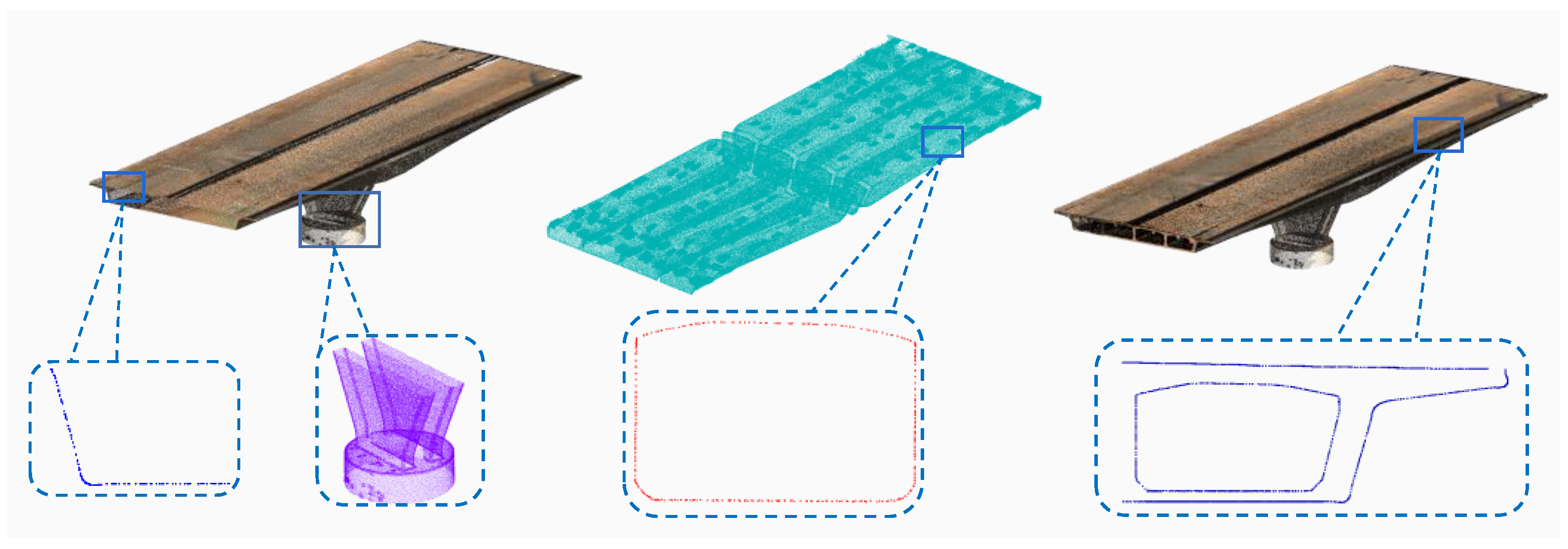
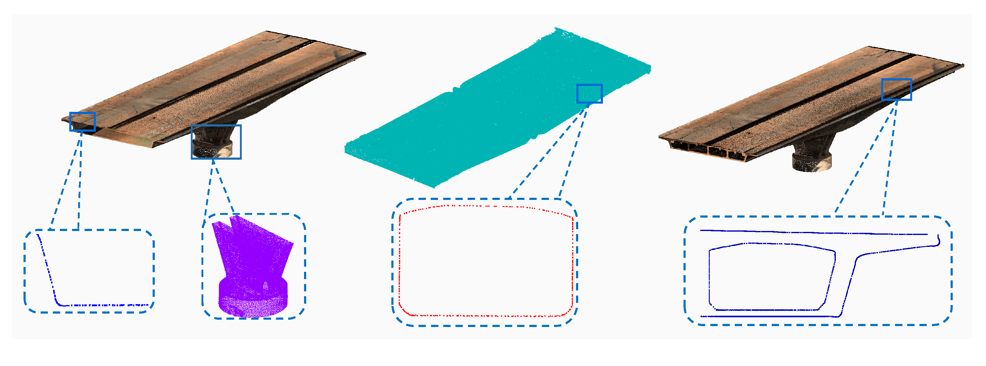
• Compared to solid section bridges, bridges with box chambers present greater challenges in point cloud data collection and registration. However, the strategic layout planning of measuring stations and targets can significantly enhance the quality and efficiency of data collection.
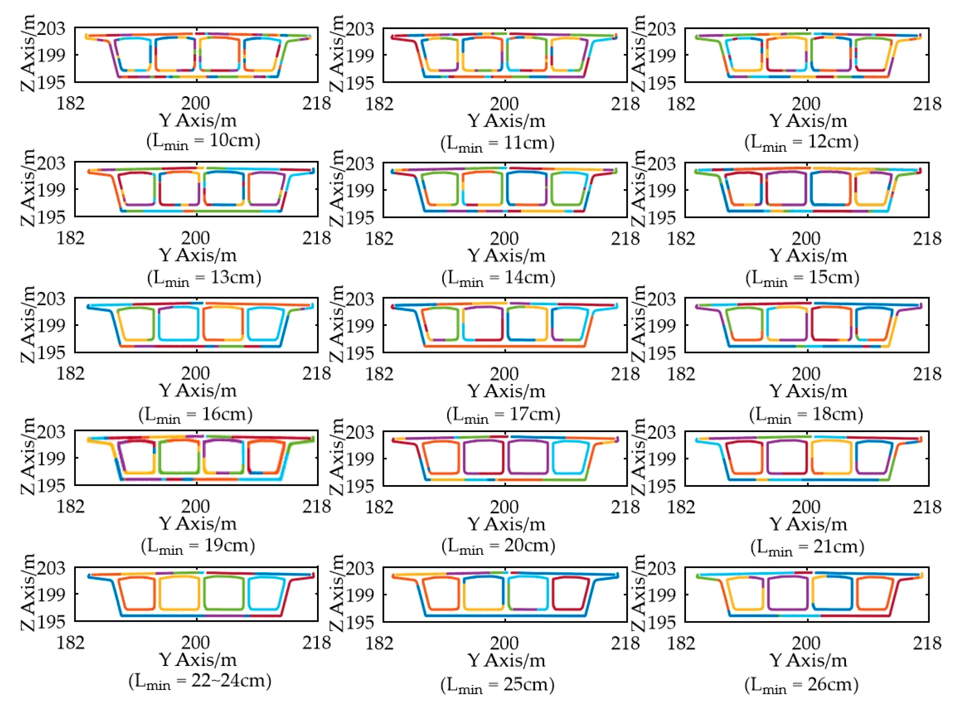
• The proposed method automates the feature extraction process from point cloud slices of the bridge box chamber contour and outer contour. This not only increases feature extraction efficiency but also ensures accurate extraction of short edges within the contour.
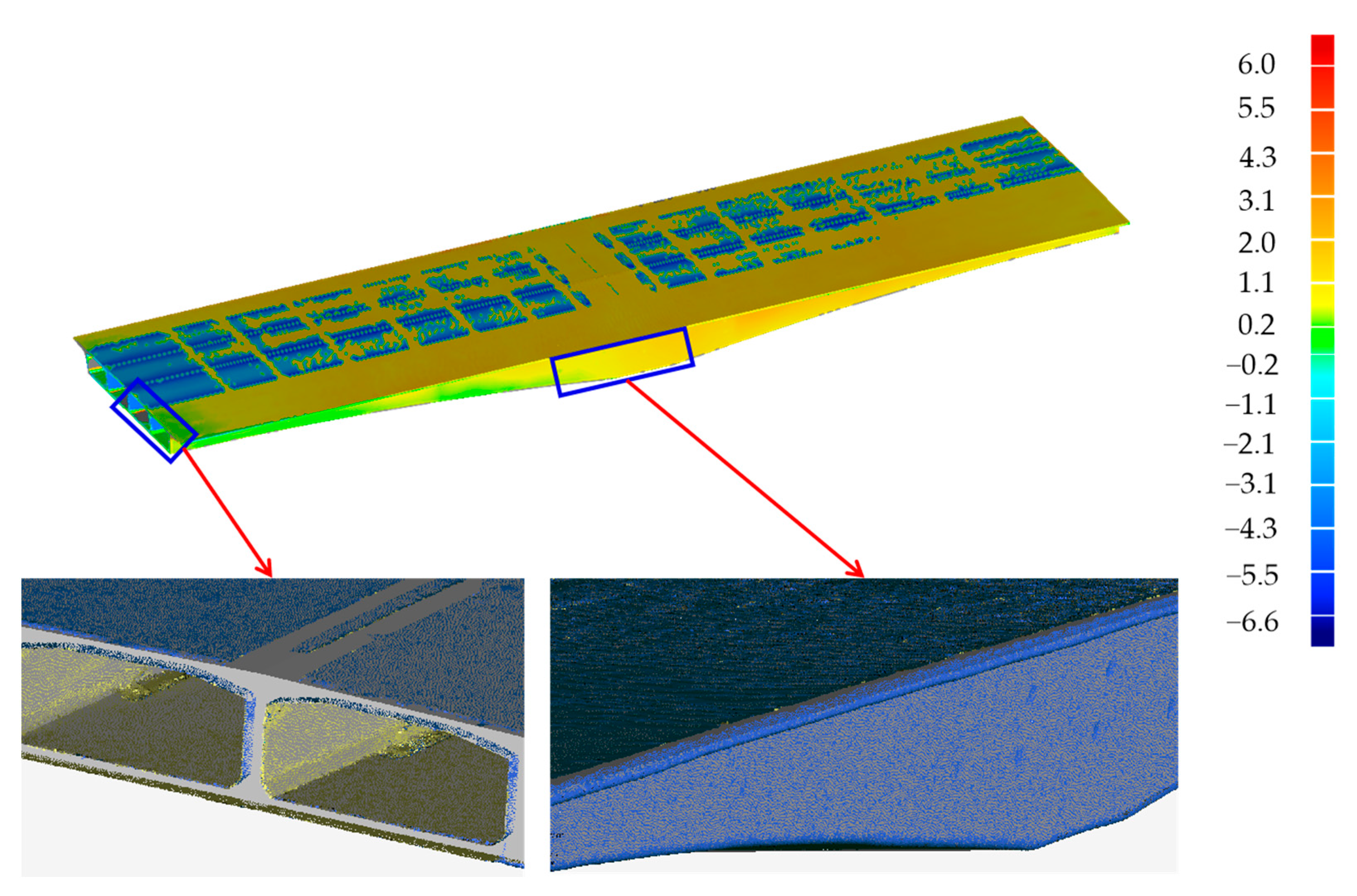
• Utilising Dynamo-Revit, the feature extraction results are directly integrated to automatically generate a bridge gDT model, thereby enhancing modelling efficiency and reducing subjective errors associated with manual operations. The accuracy of feature extraction and reverse modelling methods is confirmed through 3D deviation analysis with the measured point cloud.

Although this study successfully and rapidly generates bridge gDT models based on TLS, the bridge sections investigated in this study consist solely of straight lines. Future research should extend the extraction methods to include other types of cross-sections, such as circular and component types composed of multiple curved segments. Moreover, integrating point cloud segmentation, feature extraction, and reverse modelling into a cohesive system could further enhance the level of automation and digitisation in construction practices.

References

1. Stavropoulos, P.; Mourtzis, D. Chapter 10—Digital Twins in Industry 4.0. In Design and Operation of Production Networks for Mass Personalization in the Era of Cloud Technology; Mourtzis, D., Ed.; Elsevier: Amsterdam, The Netherlands, 2022; pp. 277–316. [Google Scholar]
2. Zhou, C.; Xiao, D.; Hu, J.; Yang, Y.; Li, B.; Hu, S.; Demartino, C.; Butala, M. An Example of Digital Twins for Bridge Monitoring and Maintenance: Preliminary Results. In Proceedings of the 1st Conference of the European Association on Quality Control of Bridges and Structures, Padua, Italy, 29 August–1 September 2021; Springer International Publishing: Cham, Switzerland, 2022; pp. 1134–1143. [Google Scholar]
3. Barazzetti, L.; Banfi, F.; Brumana, R.; Previtali, M.; Roncoroni, F. BIM from laser scans… not just for buildings: Nurbs-based parametric modeling of a medieval bridge. ISPRS Ann. Photogramm. Remote Sens. Spat. Inf. Sci. 2016, III-5, 51–56. [Google Scholar] [CrossRef]
4. Martini, A.; Tronci, E.M.; Feng, M.Q.; Leung, R.Y. A computer vision-based method for bridge model updating using displacement influence lines. Eng. Struct. 2022, 259, 114129. [Google Scholar] [CrossRef]
5. Ma, Z.; Liu, S. A review of 3D reconstruction techniques in civil engineering and their applications. Adv. Eng. Inform. 2018, 37, 163–174. [Google Scholar] [CrossRef]
6. Cheng, G.; Liu, J.; Li, D.; Chen, Y.F. Semi-Automated BIM Reconstruction of Full-Scale Space Frames with Spherical and Cylindrical Components Based on Terrestrial Laser Scanning. Remote Sens. 2023, 15, 2806. [Google Scholar] [CrossRef]
7. Han, Y.; Feng, D.; Wu, W.; Yu, X.; Wu, G.; Liu, J. Geometric shape measurement and its application in bridge construction based on UAV and terrestrial laser scanner. Autom. Constr. 2023, 151, 104880. [Google Scholar] [CrossRef]
8. Mohammadi, M.; Rashidi, M.; Mousavi, V.; Yu, Y.; Samali, B. Application of TLS Method in Digitization of Bridge Infrastructures: A Path to BrIM Development. Remote Sens. 2022, 14, 1148. [Google Scholar] [CrossRef]
9. Rashidi, M.; Mohammadi, M.; Sadeghlou Kivi, S.; Abdolvand, M.M.; Truong-Hong, L.; Samali, B. A Decade of Modern Bridge Monitoring Using Terrestrial Laser Scanning: Review and Future Directions. Remote Sens 2020, 12, 3796. [Google Scholar] [CrossRef]
10. Goebbels, S. 3D Reconstruction of Bridges from Airborne Laser Scanning Data and Cadastral Footprints. J. Geovisualization Spat. Anal. 2021, 5, 10. [Google Scholar] [CrossRef]
11. Hu, K.; Han, D.; Qin, G.; Zhou, Y.; Chen, L.; Ying, C.; Guo, T.; Liu, Y. Semi-automated Generation of Geometric Digital Twin for Bridge Based on Terrestrial Laser Scanning Data. Adv. Civ. Eng. 2023, 2023, 6192001. [Google Scholar] [CrossRef]
12. Song, X.; Jüttler, B. Modeling and 3D object reconstruction by implicitly defined surfaces with sharp features. Comput. Graph. 2009, 33, 321–330. [Google Scholar] [CrossRef]
13. Lu, R.; Brilakis, I. Digital twinning of existing reinforced concrete bridges from labelled point clusters. Autom. Constr. 2019, 105, 102837. [Google Scholar] [CrossRef]
14. Kwon, S.-W.; Bosche, F.; Kim, C.; Haas, C.T.; Liapi, K.A. Fitting range data to primitives for rapid local 3D modeling using sparse range point clouds. Autom. Constr. 2004, 13, 67–81. [Google Scholar] [CrossRef]
15. Oesau, S.; Lafarge, F.; Alliez, P. Indoor scene reconstruction using feature sensitive primitive extraction and graph-cut. ISPRS J. Photogramm. Remote Sens. 2014, 90, 68–82. [Google Scholar] [CrossRef]
16. Chen, J.; Zhang, C.; Tang, P. Geometry-based optimized point cloud compression methodology for construction and infrastructure management. In Proceedings of the Computing in Civil Engineering, Seattle, WA, USA, 25–27 June 2017; pp. 377–385. [Google Scholar]
17. Carr, J.C.; Beatson, R.K.; McCallum, B.C.; Fright, W.R.; McLennan, T.J.; Mitchell, T.J. Smooth surface reconstruction from noisy range data. In Proceedings of the Conference on Computer Graphics and Interactive Techniques in Australasia and Southeast Asia, Melbourne, Australia, 11–14 February 2003. [Google Scholar]
18. Deng, Y.; Cheng, J.C.P.; Anumba, C. Mapping between BIM and 3D GIS in different levels of detail using schema mediation and instance comparison. Autom. Constr. 2016, 67, 1–21. [Google Scholar] [CrossRef]
19. Patil, A.K.; Holi, P.; Lee, S.K.; Chai, Y.H. An adaptive approach for the reconstruction and modeling of as-built 3D pipelines from point clouds. Autom. Constr. 2017, 75, 65–78. [Google Scholar] [CrossRef]
20. Schnabel, R.; Wahl, R.; Klein, R. Efficient RANSAC for Point-Cloud Shape Detection. In Computer Graphics Forum; Blackwell Publishing Ltd.: Oxford, UK, 2007; Volume 26. [Google Scholar]
21. Xiao, J.; Furukawa, Y. Reconstructing the World’s Museums. Int. J. Comput. Vis. 2014, 110, 243–258. [Google Scholar] [CrossRef]
22. Budroni, A.; Boehm, J. Automated 3D Reconstruction of Interiors from Point Clouds. Int. J. Archit. Comput. 2010, 8, 55–73. [Google Scholar] [CrossRef]
23. Ochmann, S.; Vock, R.; Wessel, R.; Klein, R. Automatic reconstruction of parametric building models from indoor point clouds. Comput. Graph. 2016, 54, 94–103. [Google Scholar] [CrossRef]
24. Borrmann, A.; Beetz, J.; Koch, C.; Liebich, T.; Muhic, S. Industry Foundation Classes: A Standardized Data Model for the Vendor-Neutral Exchange of Digital Building Models. In Building Information Modeling: Technology Foundations and Industry Practice; Borrmann, A., König, M., Koch, C., Beetz, J., Eds.; Springer International Publishing: Cham, Switzerland, 2018; pp. 81–126. [Google Scholar]
25. Dou, S.; Zhang, X.Y. Research on Generalization Technology of Spatial Line Vector Data. Appl. Mech. Mater. 2014, 687–691, 1153–1156. [Google Scholar]
26. Marani, R.; Renó, V.; Nitti, M.; D’orazio, T.; Stella, E. A Modified Iterative Closest Point Algorithm for 3D Point Cloud Registration. Comput.-Aided Civ. Infrastruct. Eng. 2016, 31, 515–534. [Google Scholar] [CrossRef]
27. Wang, X.; Chen, H.; Wu, L. Feature extraction of point clouds based on region clustering segmentation. Multimed. Tools Appl. 2020, 79, 11861–11889. [Google Scholar] [CrossRef]
28. Lee, K.-H.; Woo, H. Direct integration of reverse engineering and rapid prototyping. Comput. Ind. Eng. 2000, 38, 21–38. [Google Scholar] [CrossRef]
29. Qiu, Y.; Zhou, X.; Qian, X. Direct slicing of cloud data with guaranteed topology for rapid prototyping. Int. J. Adv. Manuf. Technol. 2011, 53, 255–265. [Google Scholar] [CrossRef]
30. Wu, Y.F.; Wong, Y.S.; Loh, H.T.; Zhang, Y. Modelling cloud data using an adaptive slicing approach. Comput. Aided Des. 2004, 36, 231–240. [Google Scholar] [CrossRef]
31. Tang, J.; Tan, J.; Du, Y.; Zhao, H.; Li, S.; Yang, R.; Zhang, T.; Li, Q. Quantifying Multi-Scale Performance of Geometric Features for Efficient Extraction of Insulators from Point Clouds. Remote Sens. 2023, 15, 3339. [Google Scholar] [CrossRef]
32. Zhou, Y.; Xiang, Z.; Zhang, X.; Wang, Y.; Han, D.; Ying, C. Mechanical state inversion method for structural performance evaluation of existing suspension bridges using 3D laser scanning. Comput.-Aided Civ. Infrastruct. Eng. 2021, 37, 650–665. [Google Scholar] [CrossRef]
33. Zolanvari, S.M.I.; Laefer, D.F. Slicing Method for curved façade and window extraction from point clouds. ISPRS J. Photogramm. Remote Sens. 2016, 119, 334–346. [Google Scholar] [CrossRef]
34. Luo, T.; Lian, Z.; Yu, H.; Liu, Y.; Li, B.-S. Reverse design based on slicing method. J. Braz. Soc. Mech. Sci. Eng. 2019, 41, 541. [Google Scholar] [CrossRef]
35. Wang, B.; Yin, C.; Luo, H.; Cheng, J.C.P.; Wang, Q. Fully automated generation of parametric BIM for MEP scenes based on terrestrial laser scanning data. Autom. Constr. 2021, 125, 103615. [Google Scholar] [CrossRef]
36. Zhao, J.; Cui, Y.; Niu, X.; Wang, X.R.; Zhao, Y.; Guo, M.; Zhang, R.B. Point cloud slicing-based extraction of indoor components. Int. Arch. Photogramm. Remote Sens. Spat. Inf. Sci. 2022, 48, 103–108. [Google Scholar] [CrossRef]
37. Tang, P.; Huber, D.; Akinci, B.; Lipman, R.; Lytle, A. Automatic reconstruction of as-built building information models from laser-scanned point clouds: A review of related techniques. Autom. Constr. 2010, 19, 829–843. [Google Scholar] [CrossRef]
38. Zhou, Y.; Han, D.; Hu, K.; Qin, G.; Xiang, Z.; Ying, C.; Zhao, L.; Hu, X. Accurate Virtual Trial Assembly Method of Prefabricated Steel Components Using Terrestrial Laser Scanning. Adv. Civ. Eng. 2021, 2021, 9916859. [Google Scholar] [CrossRef]
39. Qin, G.; Zhou, Y.; Hu, K.; Han, D.; Ying, C. Automated Reconstruction of Parametric BIM for Bridge Based on Terrestrial Laser Scanning Data. Adv. Civ. Eng. 2021, 2021, 8899323. [Google Scholar] [CrossRef]
40. Agapaki, E.; Brilakis, I. State-of-Practice on As-Is Modelling of Industrial Facilities. In Workshop of the European Group for Intelligent Computing in Engineering; Springer International Publishing: Cham, Switzerland, 2018; pp. 103–124. [Google Scholar]
41. Son, H.; Bosché, F.; Kim, C. As-built data acquisition and its use in production monitoring and automated layout of civil infrastructure: A survey. Adv. Eng. Inform. 2015, 29, 172–183. [Google Scholar] [CrossRef]
42. Macher, H.; Landes, T.; Grussenmeyer, P. From Point Clouds to Building Information Models: 3D Semi-Automatic Reconstruction of Indoors of Existing Buildings. Appl. Sci 2017, 7, 1030. [Google Scholar] [CrossRef]
43. Azhar, S.; Khalfan, M.M.A.; Maqsood, T. Building information modelling (BIM): Now and beyond. Australas. J. Constr. Econ. Build. 2012, 12, 15–28. [Google Scholar] [CrossRef]
44. Gao, T.; Akinci, B.; Ergan, S.; Garrett, J.H. Constructing as-is BIMs from progressive scan data. Gerontechnology 2012, 11, 75. [Google Scholar]
45. Li, S.; Isele, J.; Bretthauer, G. Proposed Methodology for Generation of Building Information Model with Laserscanning. Tsinghua Sci. Technol. 2008, 13, 138–144. [Google Scholar] [CrossRef]
46. Fang, W.; Huang, X.; Zhang, F.; Li, D. Intensity correction of terrestrial laser scanning data by estimating laser transmission function. IEEE Trans. Geosci. Remote Sens. 2015, 53, 942–951. [Google Scholar] [CrossRef]
47. Kaasalainen, S.; Jaakkola, A.; Kaasalainen, M.; Krooks, A.; Kukko, A. Analysis of incidence angle and distance effects on terrestrial laser scanner intensity: Search for correction methods. Remote Sens. 2011, 3, 2207–2221. [Google Scholar] [CrossRef]
48. Kaasalainen, S.; Krooks, A.; Kukko, A.; Kaartinen, H. Radiometric calibration of terrestrial laser scanners with external reference targets. Remote Sens. 2009, 1, 144–158. [Google Scholar] [CrossRef]
Figure 1. Proposed process for generating bridge gDT model.
Remotesensing 15 04440 g001
Figure 2. Point cloud data collection process.
Remotesensing 15 04440 g002
Figure 3. Schematic diagrams of the principle for calculating the distance between the scanner and the target: (a) the constant beam height section and (b) the variable beam height section. To quickly calculate b j , make b i + 1 =   b i . α is the angle between the incident light and the normal of the target plane. The red wireframe represents Section 1, and the dark blue wireframe represents Section 2. The purple line represents the top surface line of the bridge’s bottom plate, whereas the yellow line represents the bottom surface of the bridge’s top plate.
Remotesensing 15 04440 g003
Figure 4. Adjacent cross-section target layout; the red dots represent spherical targets.
Remotesensing 15 04440 g004
Figure 5. Method for calculating the distance between adjacent bridge deck scanner stations.
Remotesensing 15 04440 g005
Figure 6. Point cloud registration process.
Remotesensing 15 04440 g006
Figure 7. Method for arranging targets and measuring stations at the internal and external point cloud registration manhole of the box chamber; (a) layout of measuring stations; (b) plane layout of targets; (c) elevation layout of targets; and (d) detailed layout of targets.
Remotesensing 15 04440 g007
Figure 8. Extraction of control points for variable cross-section sections in the bridge box chamber: (a) slicing the bridge perpendicular to the z-axis; (b) point cloud slicing containing complete box chamber contours; (c) selected box chamber contour; and (d) solution of variable cross-section control points.
Remotesensing 15 04440 g008
Figure 9. Extraction of control points for beam height variation segments; (a) slice perpendicular to the y-axis; (b) slice the longitudinal centreline of the bridge; and (c) solution of variable cross-section control points.
Remotesensing 15 04440 g009
Figure 10. Schematic diagram of bridge point cloud slicing; (a) variable cross-section segment division; (b) point cloud slicing; and (c) slicing projection.
Remotesensing 15 04440 g010
Figure 11. Inner and outer contour segmentation based on Euclidean clustering algorithm; (a) failure to select correct L m i n point cloud clustering; (b) selection of correct L m i n point cloud clustering; (c) outer contour of section; and (d) inner contour of section.
Remotesensing 15 04440 g011
Figure 12. Schematic diagram of grid segmentation: (a) grid segmentation and (b) grid filtering.
Remotesensing 15 04440 g012
Figure 13. Cross-section feature extraction steps.
Remotesensing 15 04440 g013
Figure 14. Dynamo–Revit generating bridge gDT model steps; (a) bridge route generation steps; (b) bridge outline generation; (c) Profile lofting fusion and Boolean operations; and (d) bridge gDT model.
Remotesensing 15 04440 g014
Figure 15. On-site status before the rotation of Dade Bridge.
Remotesensing 15 04440 g015
Figure 16. Layout of TLS and spherical targets. Red dots represent spherical target, and dark blue represents scanner.
Remotesensing 15 04440 g016
Figure 17. Raw point cloud: (a) point cloud below the bridge and (b) point cloud of deck; the green and purple point clouds come from different stations.
Remotesensing 15 04440 g017
Figure 18. Registered bridge point cloud model and details.
Remotesensing 15 04440 g018
Figure 19. Point clouds at different slice positions (x-axis) along the longitudinal bridge: (a) point cloud slicing for region 1; (b) point cloud slicing for region 2; (c) point cloud slicing of region 3; (d) point cloud slicing of region 4; and (e) point cloud slicing for region 5.
Remotesensing 15 04440 g019
Figure 20. Feature extraction process for swivel bridge point cloud: (a) clustering and segmentation of inner and outer contours; (b) feature extraction of point cloud; and (c) cross-section and detail of feature extraction.
Remotesensing 15 04440 g020
Figure 21. gDT model of swivel bridge.
Remotesensing 15 04440 g021
Figure 22. Chromatogram of main beam deviation, unit: mm.
Remotesensing 15 04440 g022
Figure 23. Segmentation effect of the inner and outer contours of point cloud sections under different values of L m i n .
Remotesensing 15 04440 g023
Disclaimer/Publisher’s Note: The statements, opinions and data contained in all publications are solely those of the individual author(s) and contributor(s) and not of MDPI and/or the editor(s). MDPI and/or the editor(s) disclaim responsibility for any injury to people or property resulting from any ideas, methods, instructions or products referred to in the content.