
Spatiotemporal Characteristics and Volume Transport of Lagrangian Eddies in the Northwest Pacific


1
State Key Laboratory of Marine Environmental Science, Center for Marine Meteorology and Climate Change, College of Ocean and Earth Sciences, Xiamen University, Xiamen 361102, China
2
Southern Marine Science and Engineering Guangdong Laboratory (Zhuhai), Zhuhai 519082, China
*
Author to whom correspondence should be addressed.
Remote Sens. 2023, 15(17), 4355; https://doi.org/10.3390/rs15174355
Submission received: 5 July 2023
/
Revised: 31 August 2023
/
Accepted: 1 September 2023
/
Published: 4 September 2023
(This article belongs to the Special Issue Remote Sensing Applications in Ocean Observation II)
Abstract
:Mesoscale eddies play a crucial role in the transport of mass, heat, salt and nutrients, exerting significant influence on ocean circulation patterns, biogeochemical processes and the global climate system. Based on Lagrangian-Averaged Vorticity Deviation (LAVD) method, this study applies 27 years (1993–2019) of geostrophic current velocity data to detect Rotationally Coherent Lagrangian Vortices (RCLVs) in the Northwest Pacific (NWP; 10°N–30°N, 115°E–155°E), with the spatiotemporal characteristics of Eulerian Sea Surface Height Eddies (SSH eddies) and RCLVs being compared. A higher number of SSH eddies and RCLVs can be observed in spring and winter, and their inter-annual variations are similar. SSH eddies show higher generation number and larger radius in the Subtropical Countercurrent region, while RCLVs occur more favorably in the ocean basin. The propagation speed distributions of both eddy types are nearly identical and decrease with increasing latitude. Due to the material coherent transport maintained by RCLVs within a finite time interval, the coherent cores of RCLVs are considerably smaller in scale as compared to those of SSH eddies. The average zonal transports induced by SSH eddies and RCLVs are estimated to be −0.82 Sv and −0.51 Sv (1 Sv = 106 m3/s), respectively. For non-overlapping SSH eddies with RCLVs, approximately 80% of the water within the eddy leaks out during the eddy’s lifespan. In the case of overlapping SSH eddies, the ratio of coherent water inside the eddy decreases with increasing radius, and the leakage rate is around 58%. Finally, an examination of 36 shedding RCLVs events from the Kuroshio near the Luzon Strait, which induce an average zonal transport of −0.14 Sv, reveals that 54% of the water within the shedding RCLVs originates from the Kuroshio.
1. Introduction
Mesoscale eddies are widely prevalent in the global oceans, typically persisting for weeks to months, with horizontal scales ranging from tens to hundreds of kilometers [1,2]. The mechanisms of eddy generation are often associated with factors such as ocean current instability, frontal instability, wind stress, wind stress curl, air–sea interactions, and topography [3,4,5,6,7,8,9]. The transports of heat, salt, water mass, chlorophyll and nutrients induced by these eddies play a vital role in modulating the structure of ocean circulation and biogeochemical processes [10,11,12], thereby impacting the heat balance of the ocean and the dynamics of the climate system [8,13,14,15,16].
The Northwest Pacific (NWP) is recognized as a prominent hotspot for eddy activity on a global scale [6,17,18]. In this region, the westward-flowing North Equatorial Current (NEC) and the eastward-flowing Subtropical Countercurrent (STCC) constitute the STCC–NEC system [17]. Additionally, the northward branch of NEC after encountering the Philippine Islands forms an energetic western boundary current known as the Kuroshio [19,20,21]. The Kuroshio, carrying a substantial amount of warm and saline Pacific water, intrudes into the South China Sea (SCS) through the Luzon Strait, exerting a strong influence on the circulation structures, ecological environment, regional climate, thermodynamics, and dynamic processes of the SCS [22,23,24,25,26].
Large-scale ocean circulation is commonly considered the primary carrier of oceanic energy and material transport [21]. However, the contribution of mesoscale eddies to the transports of heat, salt and water cannot be neglected compared to background advection [1,14,15]. On the one hand, eddy-induced heat and salt flux anomalies either partially compensate or cancel out for the material transport from the circulation [12,27], particularly in the Southern Ocean and western boundary regions [28,29], indicating the mixing processes associated with mesoscale eddies. On the other hand, considering the nonlinear characteristics of eddies, Dong et al. [30] estimated the meridional eddy-induced heat and salt transport using satellite altimetry data combined with Argo profiles, highlighting the dominance of individual eddy movements in oceanic heat and salt transport. Zhang et al. [31] utilized potential vorticity contours to identify eddy structures, suggesting that the eddy-induced zonal volume transport is 30 Sv (1 Sv = 106 m3/s) or greater in the NWP, comparable to the transport of large-scale wind-driven circulation. Notably, the exchange of substances between the NWP and the SCS near the Luzon Strait appears intricately linked to the eddy activity [32,33]. Shedding eddies, generated through the frontal instability caused by different types of Kuroshio’s intrusion paths in the northwest Luzon Strait, propagate westward [9,34,35,36], regulating the hydrodynamics and circulation between the NWP and the SCS [37,38]. Satellite altimetry and in situ measurements documented that the volume transport caused by shedding eddies ranges from 0.23 Sv to 0.38 Sv, accounting for 5% to 20% of the upper-layer transport through the Luzon Strait [39,40,41]. These results are all from the Eulerian perspective.
However, recent investigations have raised concerns on diagnosing eddy transport capabilities by the Eulerian method [42,43,44,45]. Techniques attempting to diagnose eddy boundaries via instantaneous Eulerian snapshots heavily rely on arbitrarily defined parameters or thresholds, especially those based on closed contours of sea surface height (SSH), commonly known as SSH eddies. These approaches introduce some biases into the results [43,46]. Moreover, the sole reliance on Eulerian features, whether instantaneous or consecutive, to establish associations among multiple entities is inadequate [47]. First, continuous features observed over the time do not necessarily pertain to the same fluid entities. Additionally, the Eulerian eddies fail to trap fluid parcels within eddy cores and maintain the coherent structures within a finite time, resulting in potential leakage errors in material transport [43,48].
Despite Eulerian eddy snapshots offering valuable insights into mesoscale dynamics [49,50,51,52], they do not fully capture the evolutionary characteristics of eddy generation and development, as well as the coherence of eddy transport. These aspects are crucial for exploring the effective transport capabilities of eddies. In contrast to the Eulerian detection methods, Lagrangian eddies are defined as fluid particles that are enclosed by material boundaries and carry internal water coherently within a finite time interval. Under the Lagrangian perspective, Haller et al. [45] introduced the Lagrangian-Averaged Vorticity Deviation (LAVD) method to detect Rotationally Coherent Lagrangian Vortices (RCLVs) that maintain material coherent transport in the ocean. The inclusion of time-dependent RCLVs trajectories significantly enhances the estimate accuracy for eddy material transport [53]. Reevaluating RCLVs in the eastern Pacific within a finite time interval, Abernathey and Haller [46] demonstrated that RCLVs with a lifespan of 30 days exhibit meridional transport peaks ranging from −0.1 Sv to −0.2 Sv, significantly lower than previous Eulerian estimates. Liu et al. [54] extracted the SSH eddies and RCLVs by using model data, revealing that the coherent core of the SSH eddies is overestimated, resulting in more than 50% of material leakage within their lifespan. The application of the LAVD method has also been extended to studying the long-lived Agulhas Rings, examining the processes of eddy generation and decay [55,56,57]. Recent studies have explored various aspects of RCLVs, including different time and spatial scales of global RCLV detection and mass transport estimation [47,58], chlorophyll convergence and divergence effects induced by RCLVs [59], and diffusivity estimation induced by RCLVs [60]. The Lagrangian approach has also been applied to estimate global ocean mixing intensity, elucidate water sources, and predict the movement of oceanic materials [61,62,63]. However, limited attention has been given to Lagrangian eddy characteristics in the active eddy zone of the NWP, and further clarification focusing on the relationship between Eulerian and Lagrangian eddies throughout their lifespans is required. Specifically, the issue of water exchange between the NWP and the SCS due to the shedding eddies from the Kuroshio near the Luzon Strait needs further investigation.
This study aims to identify RCLVs with material coherent transport capabilities using the LAVD method proposed by Haller et al. [45]. The objective is to reevaluate the water transport of eddies in the NWP, to gain a comprehensive understanding of water exchange induced by shedding eddies from the Kuroshio, and to improve the accuracy of diagnosing eddy transport capabilities. In contrast to Liu et al. [54], this paper utilizes satellite altimetry data for RCLV identification and tracking, providing a more realistic depiction of RCLV characteristics in the NWP. The rest of this paper is organized as follows: Section 2 briefly introduces the datasets and the methodology for identifying SSH eddies and RCLVs. In Section 3.1, we analyze and compare the spatiotemporal distributions of SSH eddies and RCLVs. In Section 3.2, we quantitatively assess the water transport capabilities of both types of eddies and examine the leakage of SSH eddies. In Section 3.3, we investigate the water sources of the shedding RCLVs in the Luzon Strait and estimate their volume transport. Finally, the discussion and conclusions are provided in Section 4.
2. Data and Methods
2.1. Data
In this study, we utilize daily absolute dynamic topography (ADT) and geostrophic current velocity data with a grid spacing of 0.25 degrees. The dataset is obtained from the Copernicus Marine and Environment Monitoring Service (CMEMS; https://data.marine.copernicus.eu/product/SEALEVEL_GLO_PHY_L4_MY_008_047/, accessed on 9 July 2022). To compare the characteristics of RCLVs, we also utilize the Mesoscale Eddy Trajectory Atlases (META3.1exp) dataset, which is produced by SSALTO/DUACS and distributed by the Archiving, Validation and Interpretation of Satellite Data in Oceanography (AVISO; https://www.aviso.altimetry.fr/, accessed on 6 June 2022), with support from the Centre National d’Études Spatiales (CNES). Our research focuses on the period from January 1993 to December 2019.
2.2. SSH Eddy Detection Method
The detection of SSH eddies is conducted using the py-eddy-tracker (PET) algorithm (https://py-eddy-tracker.readthedocs.io/en/stable/index.html, accessed on 29 July 2022) proposed by Mason et al. [64], which relies on the ADT as the background field. A first-order Lanczos filter with a half-power cutoff wavelength of 700 km is applied to smooth the ADT, yielding the grid data containing mesoscale variations. The eddy detection employs the ADT closed contour method, considering the specific conditions of the NWP. The following constraints are applied:
- (1)
- The daily ADT background fields are scanned with an output interval of 0.2 cm to ensure that each anticyclonic (cyclonic) eddy contains no more than one local ADT maximum (minimum). The extreme point is considered as the eddy center.
- (2)
- The amplitude is defined as the height difference between extreme point and the outermost closed contour.
- (3)
- The radius is determined as the standard circle radius with the same enclosed area as the contour. The overlapping area between the circle and the contour should be at least 30% of the eddy area.
- (4)
- The outermost contour is a single connected region containing at least 5 and at most 1000 pixels.
For SSH eddy tracking, the overlap method described in Pegliasco et al. [65] is utilized:
where represents the time step or time interval. The facilitates determining whether two eddies of the same polarity at times and are the same. If the is greater than 5%, the eddy candidates between two maps are defined as the same eddies. In case of multiple candidate eddies, the one with a higher overlap is retained. If no overlap exceeding 5% is found at the next time step, a new SSH eddy is identified. For the full explanation about this tracking scheme, please refer to Pegliasco et al. [65].
2.3. RCLV Detection Method
Within fluidic domains, Lagrangian eddies manifest as the rotating structures where the enclosed fluid parcels exhibit not only uniform rotation around their central cores at an equivalent average angular velocity, but maintain a relatively consistent motion over a finite-time interval. A prominent technique employed for identifying the boundaries of such coherently rotating structure is the LAVD method proposed by Haller et al. [45]. By quantifying the accumulative rotation angle of each fluid parcel through the calculation of relative vorticity variations over a specific time interval, the LAVD method enables the detection of RCLVs from Lagrangian trajectory data. A brief overview of the LAVD calculation is provided as follows [66].
In a two-dimensional flow field, the instantaneous relative vorticity is given by
Relative to the entire flow field, the vorticity anomaly for each particle can be expressed as the instantaneous relative vorticity minus the spatial average of the entire field:
Subsequently, the average of the vorticity anomalies along the particle’s trajectory yields the LAVD:
In Equation (2), and represent the velocity and vorticity of a particle ( at time , respectively. In Equation (3), and represent the vorticity anomaly of a particle ( at time and the time-averaged vorticity of all particles at time , respectively. In Equation (4), and represent the starting and ending time, respectively. represents the vorticity anomaly of a particle initially located at at time .
Therefore, RCLVs can be considered as an assembly of particles exhibiting comparable rotational characteristics within a finite time interval, and the boundaries of RCLVs can be identified as closed contour lines of LAVD at each interval. The procedure for detecting RCLVs based on the LAVD results is as follows [45]:
- (1)
- Selecting a finite time interval T = [t0, t1], the LAVD field is computed using Equation (4).
- (2)
- The center of the RCLVs is defined as the local maximum of LAVD.
- (3)
- The regions of RCLVs are grown by iterating through the nested contour field around the center. The boundaries of RCLVs are the outermost closed contour of LAVD.
- (4)
- The vorticity of RCLVs > 0 for anticyclonic eddies (ACEs), and else for cyclonic eddies (CEs) in the Northern Hemisphere.
- (5)
- The amplitude and the radius of RCLVs are determined in the same manner as SSH eddies.
- (6)
- The increment of the numerically calculated LAVD contour will distort the convex hull of the RCLV boundary. To ensure the coherence and convexity of the RCLV boundaries, the requirements of the Coherency Index (CI) and Convexity Deficiency (CD) are introduced:
- i.
- The CD is defined as the ratio of the difference in the area between the convex hull and the contour to the area enclosed by the contour’s area [45]. Higher CD values indicate more filamentary tails and less compact geometry. And the closer CD is to zero, the closer the eddy boundary is to become a convex curve.
- ii.
- The CI examines the change in the spatial compactness of particles inside the contour over a finite time interval T = [t0, t1], which is expressed from the variance of the particle positions (σ2(t)):
The CI is then calculated as the relative change in compactness between the starting time t0 and ending time t1:
where 〈 〉 indicates an average over the set of RCLV particles and | | is the standard Euclidean distance. The sign and magnitude of CI specify the material coherency of an RCLV. A positive CI value (CImax = 1) indicates that the RCLV is strongly coherent. The CI metric penalizes an RCLV for dispersing and developing filaments, and rewards an RCLV for growing more compact.
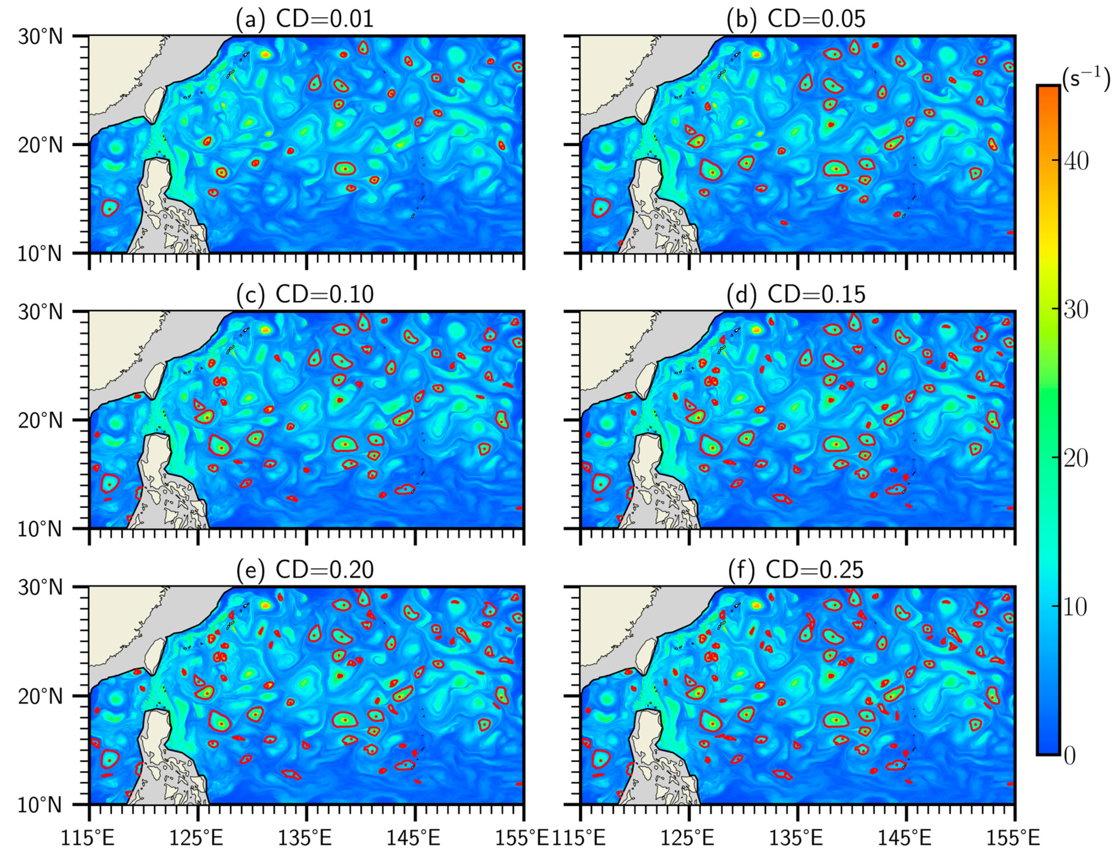
Building upon the work of Tarshish et al. [67], we provide a comprehensive exposition and exemplification of the structures of the RCLVs. Figure 1 illustrates the distribution and boundaries of the identified RCLVs at varying CD values. It is evident that smaller CD values hinder the stretching of eddies, leading to a reduction in the quantity of RCLVs. This implies that this criterion is so strict that prevents the identification of coherent structures. As CD values increase, the number of RCLVs gradually increases along with their size. For CD > 0.15, the RCLVs’ abundance becomes stable, yet their boundaries start to deform, indicating incoherence of RCLVs over the time. Hence, drawing from sensitivity experiments conducted in previous studies [45,66,67], we choose CD < 0.1 and CI > −1 as the thresholds in this study. Although it is imperative to rigorously select parameters to constrain the structure of RCLVs, we still expect to detect a substantial number of coherent structures.
In this work, the LAVD field is computed by the numerical integration of artificially released Lagrangian particles in the oceanic velocity field over a finite time interval. A grid particle matrix is uniformly initialized with a horizontal resolution of 1/32° × 1/32°. A smaller spatial resolution compared to the velocity field enables more detailed information of oceanic features [45]. The particle trajectories are then propelled by fourth-order Runge–Kutta integration in time, mapping the particles’ spatial paths and tracking the vorticity matrices of each particle. The instantaneous vorticity deviation is obtained by subtracting the average vorticity of all particles at the same time, resulting in the LAVD field over the specified time interval. The Lagrangian particle tracking toolbox and documentation can be found on the Ocean Parcels website (https://oceanparcels.org/, accessed on 10 October 2022). The algorithm for LAVD computation and RCLVs detection is provided as an open-source Python code available at GitHub (https://github.com/rabernat/floater/, accessed on 12 November 2022).
3. Results
Based on the methodology described above, we conduct a comprehensive analysis of SSH eddies and RCLVs in the NWP (10°N–30°N, 115°E–155°E) with a lifetime of 30 days during 1993–2019. A key distinction of RCLVs, in comparison to SSH eddies, lies in their identifications within a specific finite time interval. So, we initialize all Lagrangian particles at the first day of every 30-day interval within the flow field. After integrating their trajectories over time, we obtain the LAVD field, and then RCLVs with a lifetime of 30 days are identified from the initialization date. In order to compare the features of SSH eddies and RCLVs in the same time interval, we also extracted SSH eddies from the META3.1exp dataset that share the same generation date as RCLVs and persist for the next 30 days. It is noted that the NWP stands as a vital geographic domain significantly impacted by tropical cyclones, which induce a strong perturbation on the sea–atmosphere interface named as near-inertial oscillations (NIOs), consequently injecting substantial momentum and energy into the ocean [68,69]. NIOs are a significant component of ocean dynamics, characterized by oscillations persisting for many days in the upper ocean before decay, with the frequency close to the local Coriolis frequency [70,71]. Previous observations and experiments indicated an intricate interaction between NIOs and mesoscale eddies, which involves a modulation effect of eddies on the frequency, propagation and thermal response of NIOs [72,73,74]. This symbiotic relationship contributes to complexities in the interpretation of SSH anomalies. It is of great importance to emphasize the potential influence emanating from NIOs. In the framework of our research, the results might include a limited portion of NIOs under realistic conditions, which will be important for a further comprehensive investigation. To ensure the robustness of the results, we mask the data for areas where the depths are shallower than 200 m, and exclude SSH eddies and RCLVs with a radius smaller than 25 km and an amplitude smaller than 2 cm.
3.1. Eddy Spatiotemporal Characteristics
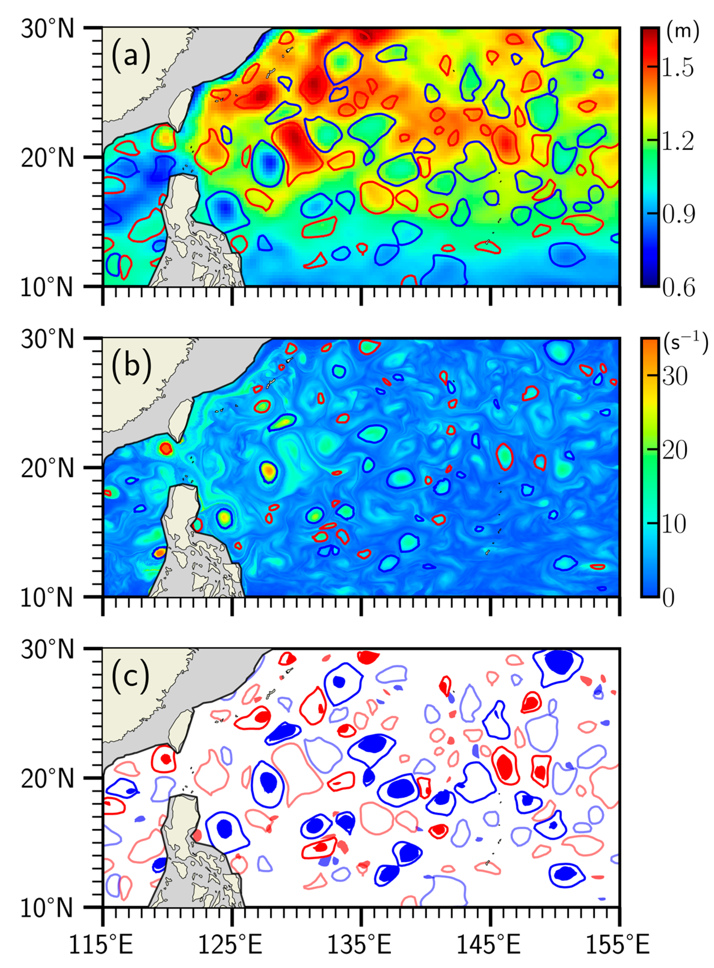
The initial positions of SSH eddies and RCLVs in the NWP on 1 January 1993, are shown in Figure 2, covered on the ADT field and LAVD field, respectively. The generation of these eddies in the region has been confirmed to be associated with barotropic or baroclinic instability [17,52] and both of them exhibit a westward propagation after generation [20,75]. It can be observed that the ACEs and CEs detected using SSH field can also be captured using the LAVD identification algorithm effectively. Some RCLVs’ boundaries (Figure 2b) exhibit filamentous and stretched structures, reflecting the fact that the coherence of RCLVs decays from the center to the outside. If the overlap area between an SSH eddy and an RCLV is more than half of either area, it is named as an overlapping SSH eddy, otherwise it is a non-overlapping SSH Eddy. Figure 2c combines the initial locations of 30-day SSH eddies (closed contours) and RCLVs (color shading), with overlapping SSH eddies and RCLVs highlighted in darker colors. Notably, most RCLVs are embedded within the SSH eddies’ core and the area of these RCLVs is considerably smaller than that of the corresponding SSH eddies.
Table 1 presents the statistics of SSH eddies and RCLVs, including number, amplitude, radius, zonal propagation speed, meridional propagation speed (, where can be zonal or meridional, and is the center position of eddy), Eddy Kinetic Energy (EKE, EKE is defined by , where and are the zonal and meridional components of the geostrophic current anomaly, respectively), and vorticity. Compared to SSH eddies, RCLVs exhibit the most prominent differences in terms of radius. Both SSH eddies and RCLVs seem to maintain larger parameter values for CEs, except for radius and meridional propagation speed.
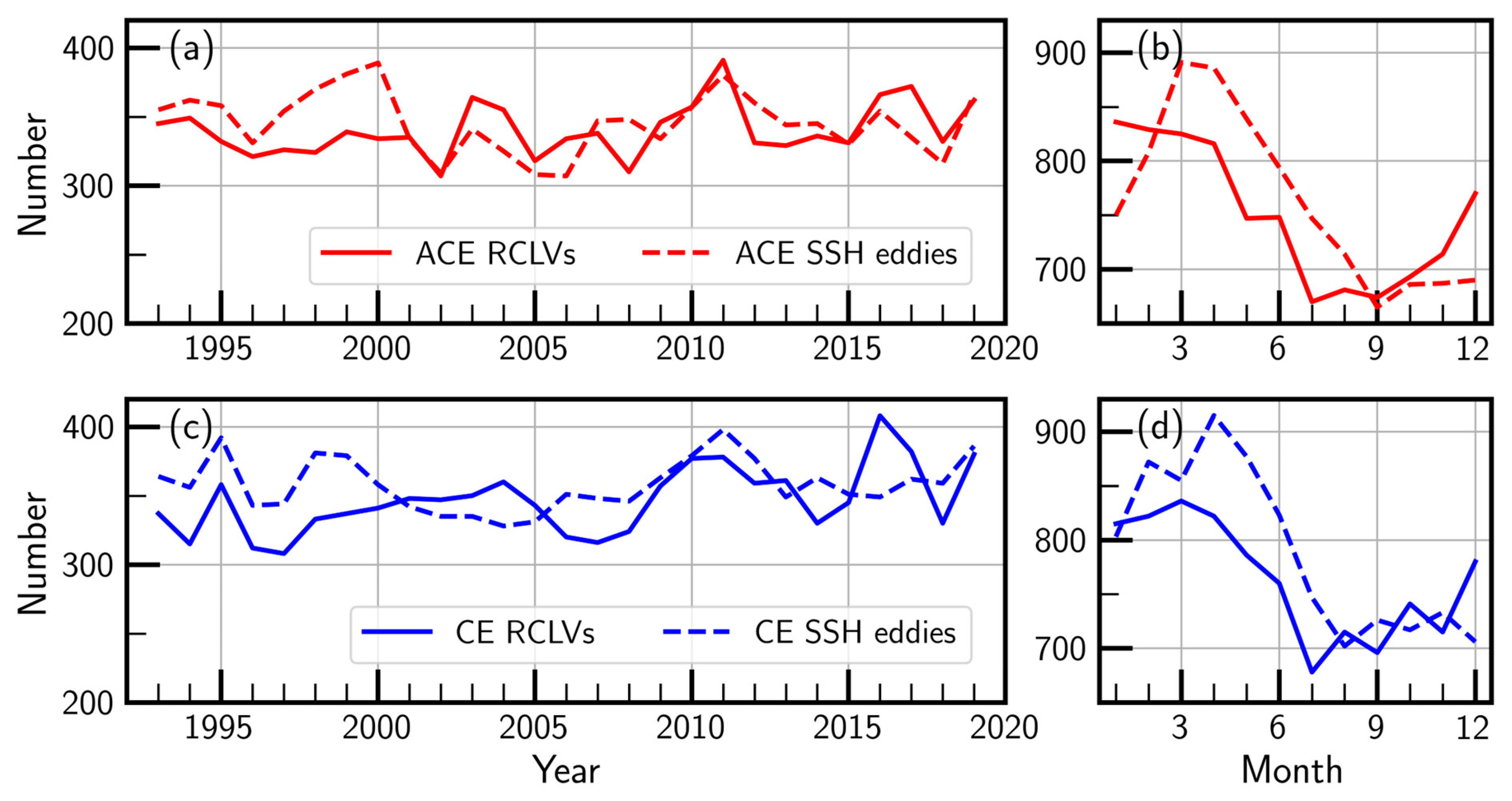
Figure 3 presents the statistical results of the total number of SSH eddies and RCLVs. Over the study period, 18,633 SSH eddies were identified, consisting of 9157 ACEs and 9476 CEs. The number of RCLVs is slightly lower, with a total of 18,169, including 9003 ACEs and 9166 CEs. Both SSH eddies and RCLVs exhibit relatively minor interannual variability, with the numbers of ACEs and CEs consistently falling within the range of 300–400. Moreover, the inter-annual variability of SSH eddies and RCLVs are similar, suggesting a potential spatiotemporal correlation with large-scale climate variability modes [7,76]. The generation of mesoscale eddies displays distinct seasonal variation, showing higher values for spring and winter, which may be attributed to intensified air–sea interactions, vertical shear, wind stress, and frontal instability [3,4,6,77,78].
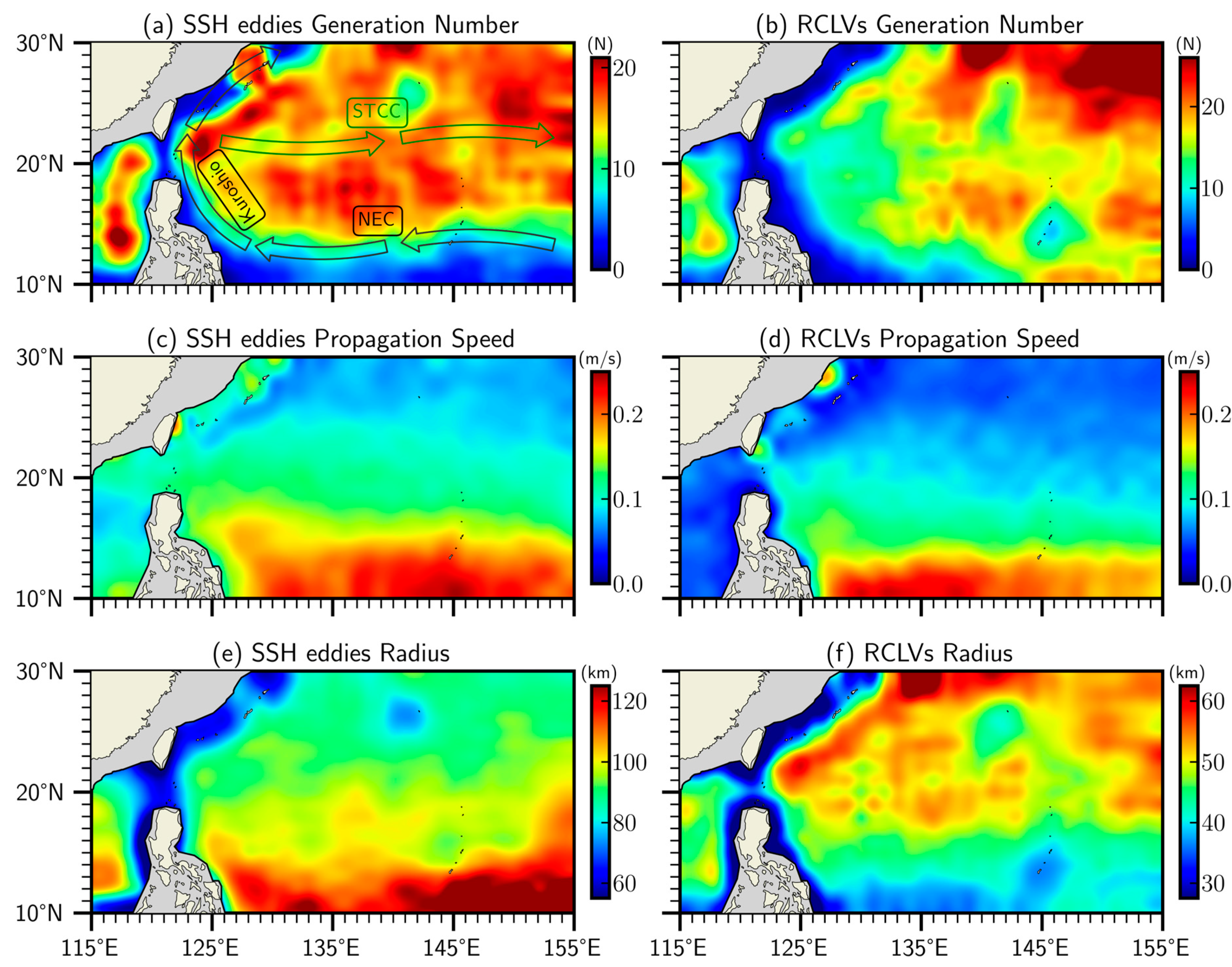
The spatial distributions of eddy generation number, propagation speed, and radius on a 1/2° × 1/2° grid are illustrated in Figure 4. One can see an evident spatial dependence in the geographical patterns of eddy generation number (Figure 4a,b) and radius (Figure 4e,f) for both SSH eddies and RCLVs. The majority of SSH eddies and RCLVs tend to concentrate in the high-latitude regions of the study area, while eddy activity is relatively lower in tropical and low-latitude regions, consistent with previous findings on the distribution of mesoscale eddies [2]. RCLVs are more abundant in the ocean basin regions, where the influence of topography on eddy occurrence diminishes, and areas with weaker flow are more conducive to the generation of stable RCLVs with coherent transport capabilities enhanced. However, the impact of the Kuroshio with its strong instability significantly hinders the evolutions of RCLVs.
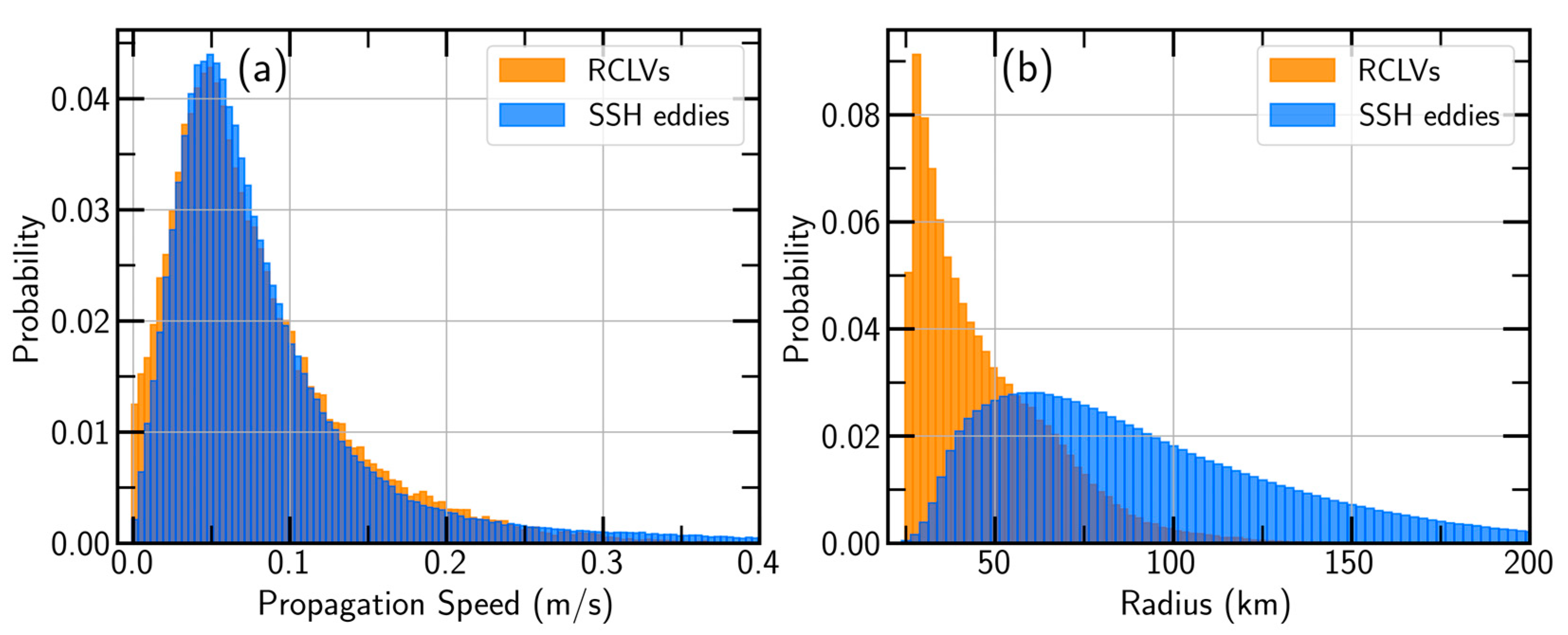
To quantify the zonal propagation tendency, we examine the westward propagation speed of eddies derived from the zonal distance travelled during their lifespans. Both SSH eddies and RCLVs demonstrate similar magnitudes and spatial distributions of the propagation speed, showing a distinct latitudinal dependence (Figure 4c,d). Eddies propagate much faster at lower latitudes, despite the fewer abundance in those regions. The radius distribution of the SSH eddies roughly follows the deformation radius of the average Rossby radius. As the latitude increases, the radii of SSH eddies generally exhibit a linear decrease (Figure 4e). Conversely, at low-latitudes, the higher flow velocity and weaker Coriolis force result in a more pronounced impact of velocity variations on RCLVs’ coherent core, leading to smaller radii of RCLVs. Additionally, we provide the probability density histograms of eddy propagation speed (Figure 5a), which clearly show that the propagation speed distributions of the two types of eddies are quite similar, with their velocity centered in the range of 0–0.1 m/s. However, a significant difference exists in the distribution of eddy radius (Figure 5b), where the radius distribution of RCLVs is more concentrated. In comparison to SSH eddies, the average radius of SSH eddies is approximately twice that of RCLVs, as RCLVs require material coherent transport.
3.2. Analysis of Eddy Transport
Let us now discuss the ability of eddies’ material transport. Due to the lack of three-dimensional eddy information, we are prompted to assume an idealized eddy model. Previous studies on global or regional mesoscale eddy profiles show that, the influence depth of eddies may range from several hundred meters to 2000 m [19,38,79,80], with larger depths in strong current regions and shallower ones in the interior of the ocean [29]. Taking these perspectives into account, here we consider a uniform influence depth to be 1000 m for all eddies in NWP. The resulting transport estimates are only accurate within an order of magnitude; further validation through quantitative data analysis is still necessary.
Assuming that SSH eddies can maintain coherent transport throughout their lifetime (RCLVs are always coherent), the volume transport () is calculated as follows [47,59]:
where and are the volume and diameter of each individual eddy, respectively; and are its zonal propagation speed and meridional propagation speed, respectively; and is the number of eddies for each 1° × 1° grid point in the study area from 1993 to 2019.
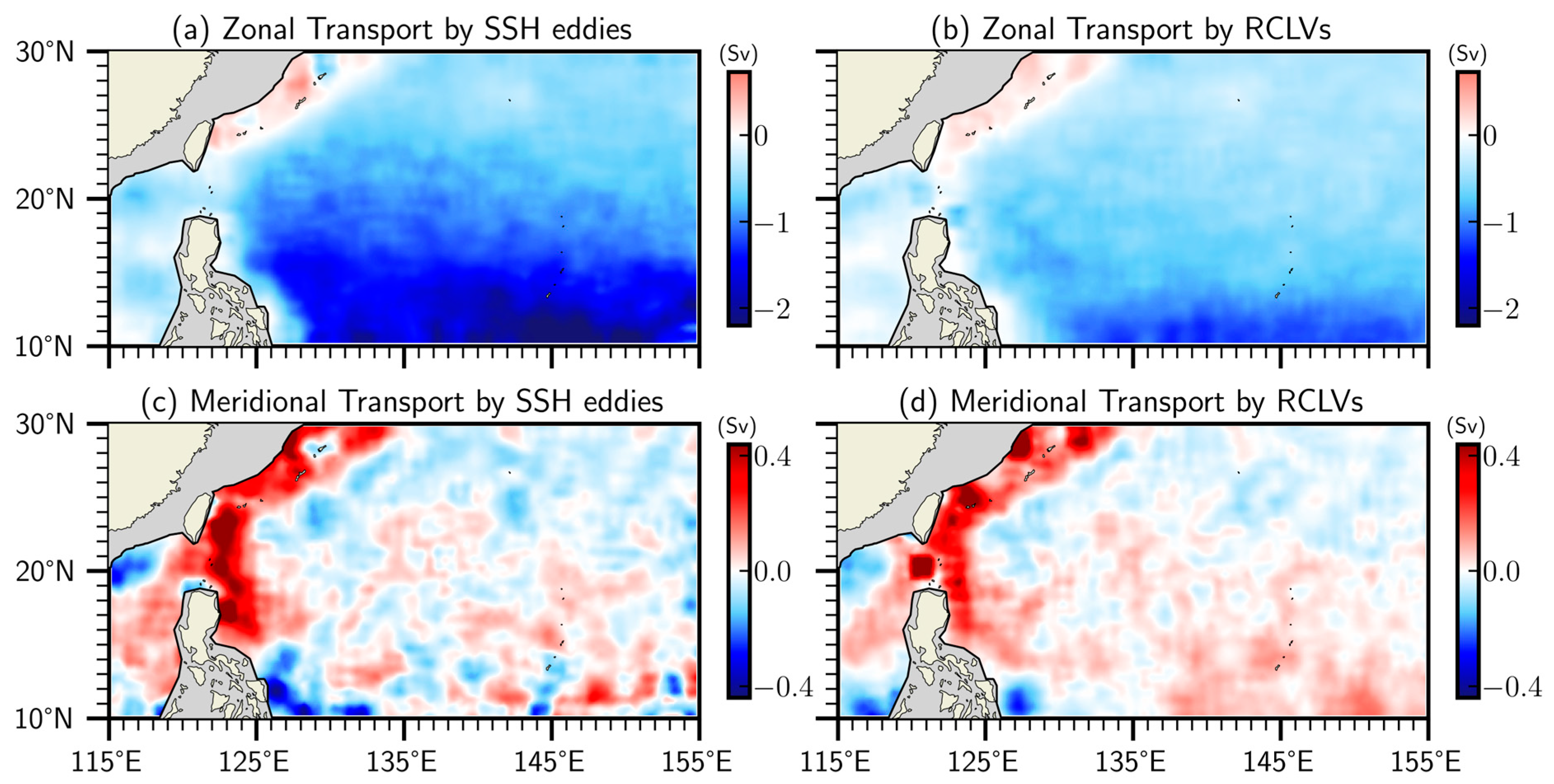
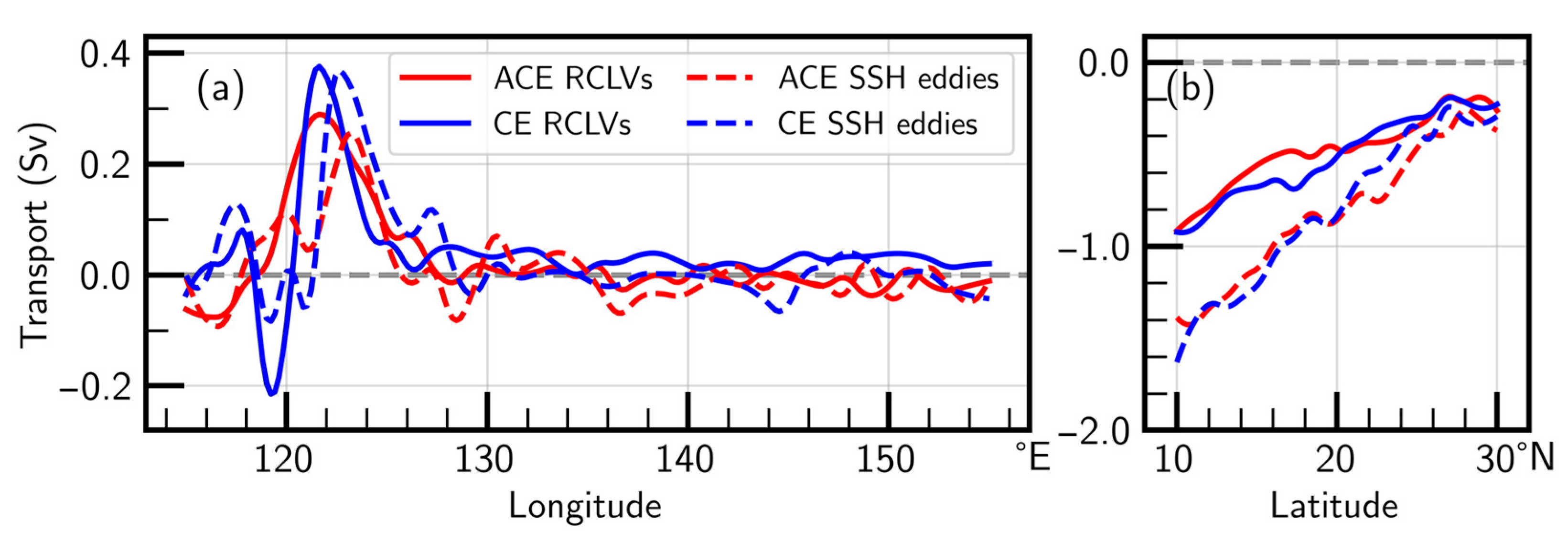
The spatial patterns of average eddy-induced transport capacity are shown in Figure 6. It is evident that both SSH eddies and RCLVs exhibit robust westward transport (the symbol ‘−’ denotes westward or southward direction). The transport of SSH eddies is more than that of RCLVs, with the average zonal transport ranging from −0.2 Sv to −1.6 Sv per degree latitude for the former and −0.2 Sv to −1.0 Sv per degree latitude for the latter. Both types of eddies show a decrease in zonal transport with increasing latitude (Figure 7b), and the spatial distribution of zonal transport (Figure 6a,b) is similar to the propagation speed distribution (Figure 4c,d), indicating a direct influence of the propagation speed distribution on transport patterns. The average eddy-induced zonal transport for all SSH eddies is estimated at −0.82 Sv, while for all RCLVs, it is estimated at −0.51 Sv. This discrepancy in transport can be primarily attributed to the contrasting radius sizes between the two types of eddies. It is worth noting that eddies primarily propagate westward after generation, resulting in stronger zonal transport than meridional transport. Furthermore, the meridional transport of eddies exhibits particularly intensity and alignment with the Kuroshio at the western boundary (Figure 6c,d and Figure 7a), reflecting the substantial impacts of the Kuroshio on eddy volume transport. In summary, the spatial distribution of eddy-induced zonal transport is closely linked to their propagation speed. While in the case of SSH eddies, the absence of the coherent transport constraint leads to larger eddy radius compared to RCLVs, resulting in higher transport estimates.
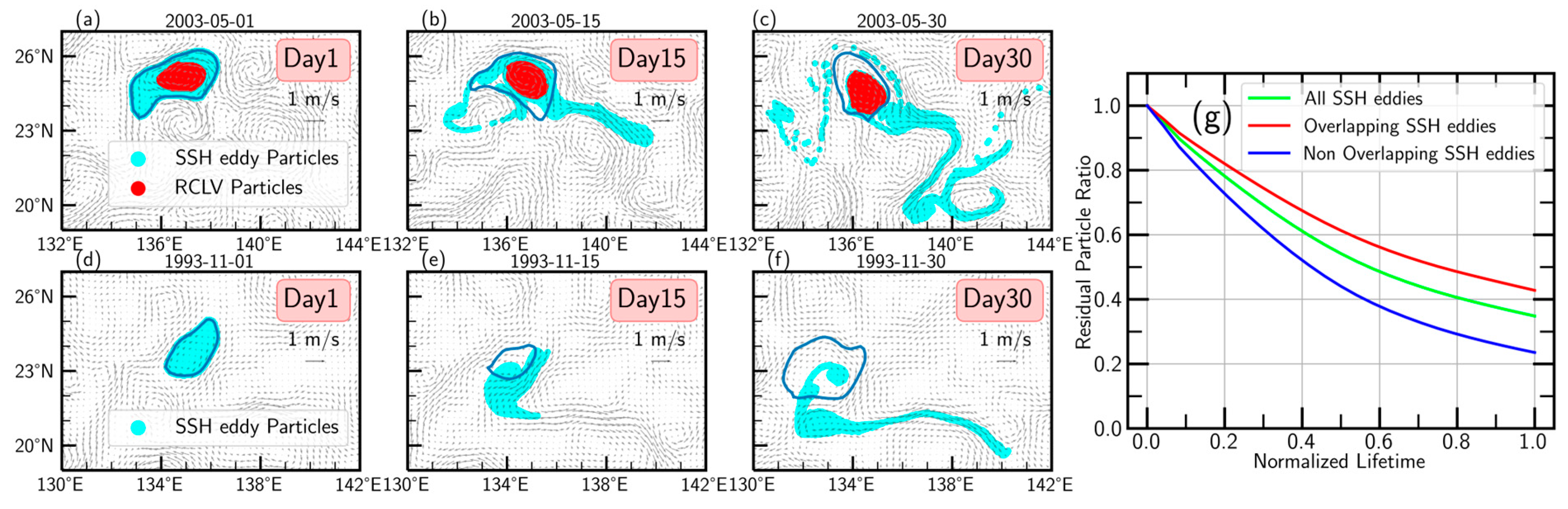
Figure 8 illustrates the leakage processes for two randomly selected cases of SSH eddies, one overlapping with RCLVs and the other non-overlapping. The water within the eddy core tends to exhibit coherent transport, and this portion is consistently identified as RCLVs (red dots in Figure 8a–c). Over the next 30 days, no particle leakage occurs within the RCLVs, as all particles remain being carried by the RCLVs, preserving their relatively stable shape. However, SSH eddies’ surrounding areas and shapes exhibit considerable variations at different time intervals, and their boundaries cannot trap the internal water effectively, particularly for the non-overlapping SSH eddies (Figure 8d–f), in which substantial intrusion of external water and leakage of internal water occur during their evolution. At the 30th day, the leakage rate is approximately 60% for overlapping SSH eddies, whereas non-overlapping SSH eddies experience a leakage ratio close to 80%, retaining only around 20% of the initial water (Figure 8g). For all SSH eddies, at least 65% of the internal water is not coherently carried by the eddies throughout their lifespan. The water enclosed by the boundaries of SSH eddies, as identified by closed contours of ADT, no longer remains constant over the time. Consequently, the eddy-induced transport derived from the Eulerian method may overestimate the real values.
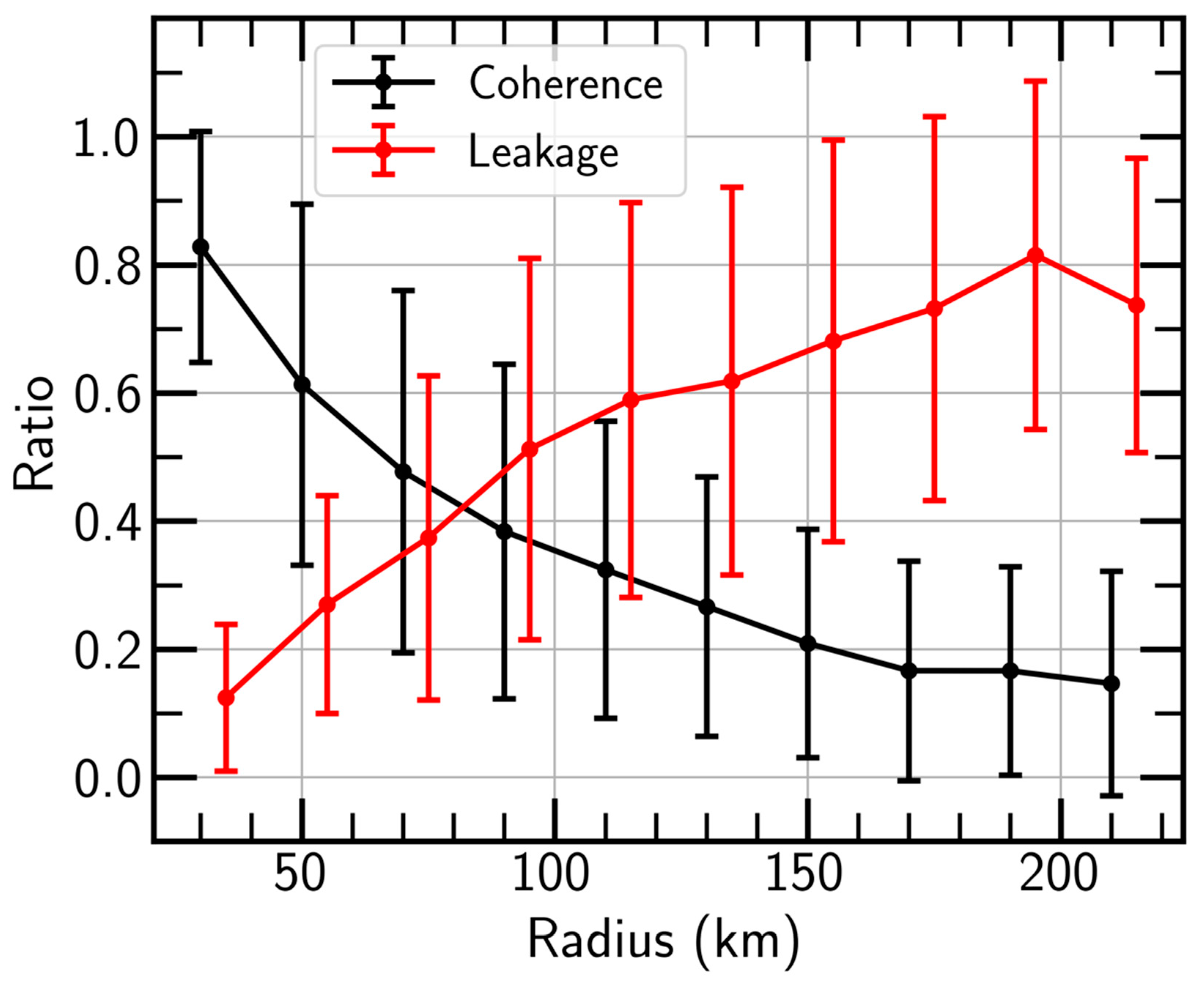
To quantitatively assess the extent of coherent water transport within overlapping SSH eddies, we analyze the variations in the ratios of the coherence and leakage of water as a function of radius (Figure 9). It is observed that as the radius increases, the ratio of coherent water within overlapping SSH eddies gradually decreases while the water leakage intensifies. Specifically, when the radius of overlapping SSH eddies reaches 200 km, the ratio of coherent water inside the eddy core reduces to less than 20%, corresponding to a mere 80% water leakage. It is worth mentioning that the sum of the ratios of coherent water and leakage water for overlapping SSH eddies is less than 1, indicating the persistence of a certain fraction of water enclosed by the evolving eddy boundaries. Although such water may not maintain coherence, they manage to avoid leakage. These findings suggest the possible inadequacy of the Eulerian method in accurately capturing the intricate properties of coherent eddy structures, especially when dealing with non-overlapping SSH eddies.
3.3. Features of Shedding RCLV in the Luzon Strait
The Luzon Strait, serving as the conveyor belt connecting the NWP and the SCS, has long obtained the interest of researchers studying the water exchange in this region. Among the various modes of water exchange, the shedding eddies induced by the Kuroshio intrusion hold significant importance, deserving careful consideration. Taking the advantage of the LAVD method in identifying coherent transport within RCLVs, it becomes possible to reevaluate the eddy-induced transport in the Luzon Strait. Building upon the selection criteria for shedding RCLVs proposed by Zhang et al. [40], an occurrence of a shedding RCLV event is defined as the ADT contours of the Kuroshio path extend west of 120°E in the northeastern SCS and then return to the NWP in a clockwise circulation through the northern Luzon Strait together with the presence of an RCLV.
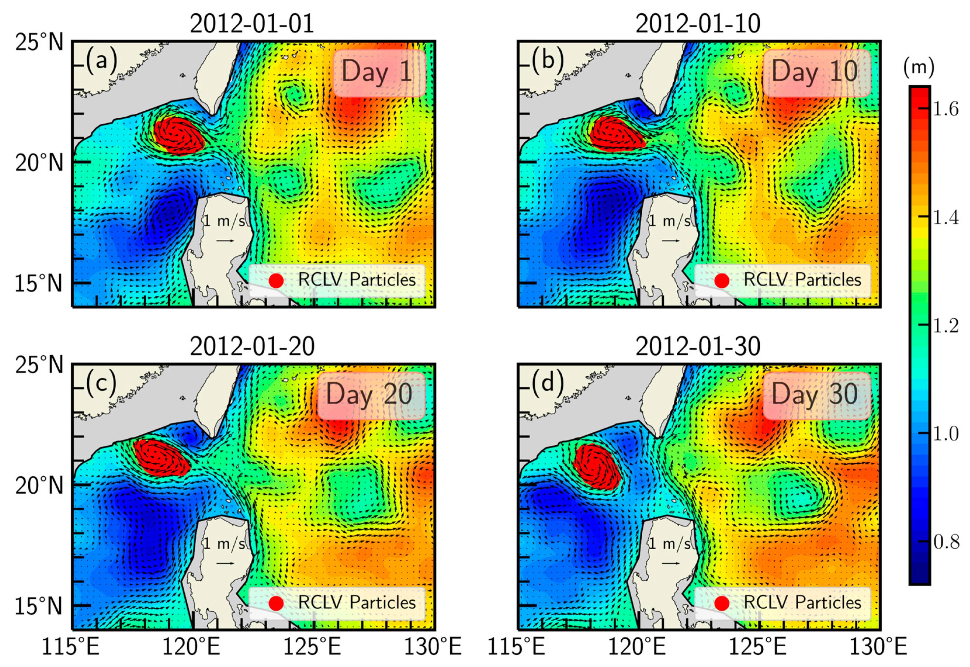
Figure 10 shows the formation of the Loop Current and the evolution of its accompanying shedding RCLV. The main axis of the Kuroshio strongly shifted toward the northwest Luzon Strait, while the shedding RCLV started to establish on 1 January 2012. Then, the intrusion of the Kuroshio continued to intensify. By 20 January 2012, the shedding RCLV moved westward with a coherent shape and gradually separated from the Kuroshio (Figure 10c). On the last day, closed ADT contours were isolated between the shedding RCLV and the Kuroshio, indicating the formation of the shedding RCLV, and the core of shedding RCLV continued to maintain a rising ADT toward the SCS.
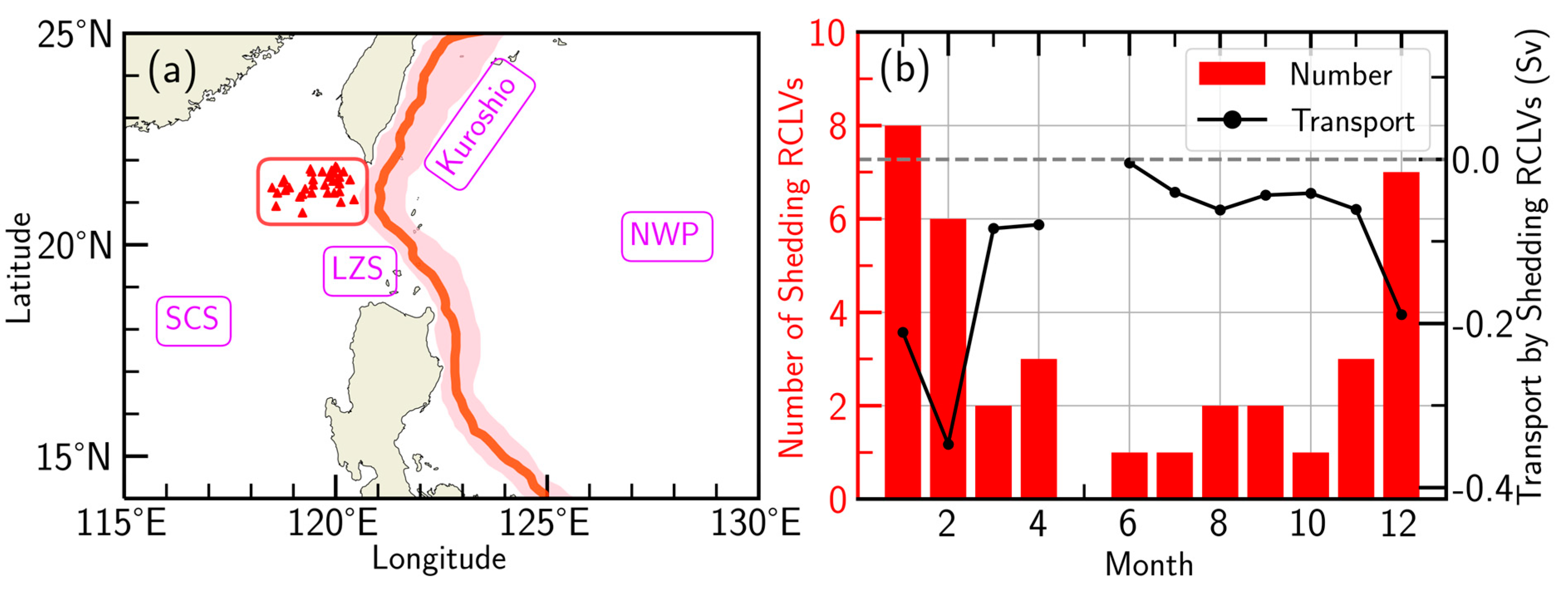
Figure 11a presents the occurrence locations of a total of 36 shedding RCLVs (all are ACEs) with a 30-day lifetime identified in the northwestern Luzon Strait during the study period from 1993 to 2019, with an average annual occurrence of 1.3 ± 1.1 events per year. Consistent with previous statistical findings [36,40,81], these RCLVs exhibit a higher occurrence rate during the autumn and winter seasons. The average eddy-induced zonal transport associated with shedding RCLVs amounts to −0.14 Sv, with the peak occurring in February at approximately −0.35 Sv (Figure 11b). Although the use of a constant eddy influence depth may introduce estimation errors, the focus of this study lies in the assessment of coherent transport induced by eddies, yielding a robust result indicating a relatively small volume transport of RCLVs. As there existed discrepancies among previous studies regarding eddy-induced transport in the Luzon Strait [39,40,41], it should be noted that their results were based on Eulerian eddy detection, which introduced uncertainties in estimating eddy radius and propagation speed. Considering the generation and evolution processes of eddies are essential, previous studies might have overestimated the real eddy-induced transport in this region.
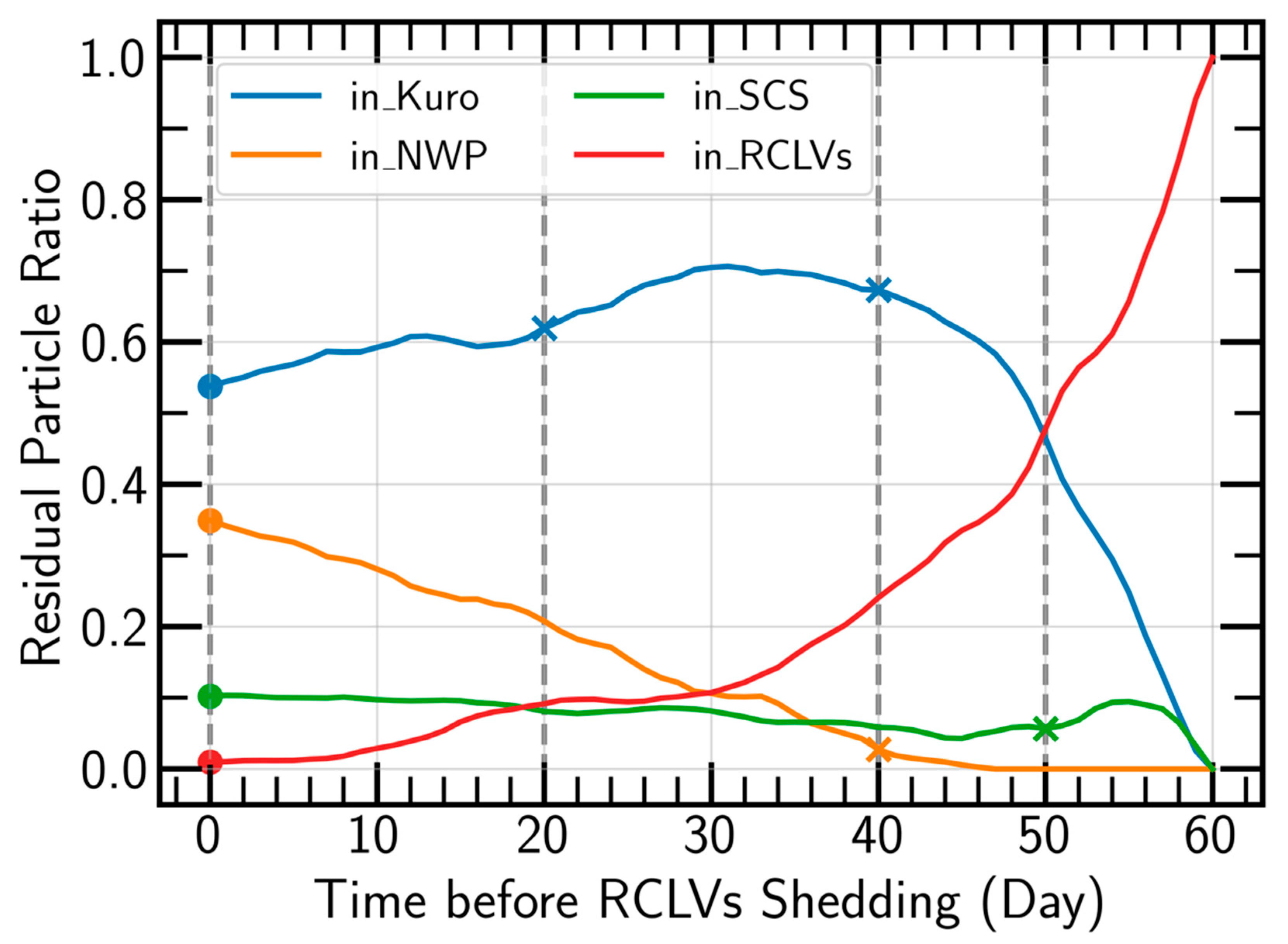
Finally, we turn to discuss the evolution of shedding RCLVs from the Kuroshio, aiming to understand the underlying processes involved in their occurrence. To explore the origin of the internal water within the shedding RCLVs, for each shedding RCLV, we uniformly release a set of Lagrangian particles at a spatial resolution of 1/32° × 1/32° within its interior. These Lagrangian particles serve as effective tracers that unravel the intricate details of the RCLVs’ shedding process. We conduct a backward time integration of these particles for 60 days, accounting for the upstream Kuroshio water into the Luzon Strait, as well as the formation of looping and shedding RCLVs. It is noted that the Kuroshio axis is defined as the position east of 120°E where the climatic average velocity reaches a maximum and the Kuroshio region is determined on either side away from the axis with a cutoff velocity greater than 0.3 m/s [82,83]. As shown in Figure 12, approximately 54% of the internal particles within the eddies originate from the Kuroshio 60 days before the occurrence of shedding RCLVs. Then, the particles residing in the NWP are gradually entrained into the Kuroshio with the Kuroshio intrusion enhancing, contributing to an increasing accumulation of particles within the Kuroshio, reaching a peak of around 70% on the 31st day after the release of particles. Subsequently, it takes about 10 days for the particles to travel through the Kuroshio towards the shedding RCLVs. The RCLVs trapping mainly occurs on the 20th day preceding the occurrence of shedding RCLVs and then the capture ratio continuously increases. A fraction of water parcels lingering in the SCS also tend to aggregate towards the shedding RCLVs. Simultaneously, it is worth noting that a cold-core eddy forms on the southwestern side of the Luzon Strait [51,63], during this period, giving rise to a north–south eddy dipole structure with the shedding RCLVs, delaying the trapped water parcels into the shedding RCLVs. Eventually, all particles merge into the interior of the shedding RCLVs and move coherently towards the SCS.
4. Discussion and Conclusions
The complicated ocean circulation structure in the NWP serves as a fertile ground for the generation of mesoscale eddies, whose transports of volume, heat, salt and nutrients exert a profound influence on oceanic physical, chemical and biological processes. Previous studies on eddies in the NWP primarily rely on Eulerian methods, which are subjective, dependent on manual parameters and thresholds, and have limitations in revealing the coherent structures of eddies over a finite time. In contrast, Lagrangian methods considering particle trajectories offer a more robust approach to identify the coherent structures of eddies. Recently, Haller et al. [45] introduced the LAVD method to examine RCLVs with material coherent transport, providing novel perspectives for studying eddies within the Lagrangian framework.
In this study, applying both the Eulerian method based on the ADT closed contour and the Lagrangian method based on the LAVD, we identify 30-day SSH eddies and RCLVs in the NWP (10°N–30°N, 115°E–155°E) from 1993 to 2019. Then, we compare their spatiotemporal characteristics, and focus on the volume transport associated with two types of eddies. The following conclusions are drawn:
During the study period, the number of SSH eddies in the NWP is slightly higher than that of RCLVs, but both exhibit similar inter-annual variability. The eddy-generation number peaks in spring and winter, with the most remarkable number differences observed between SSH eddies and RCLVs during these two seasons. Compared to SSH eddies, RCLVs are less abundant in the Kuroshio region and have a significantly smaller radius, approximately half the size of SSH eddies. The magnitudes and spatial distributions of propagation speed of the two types of eddies are similar. Assuming the coherence of SSH eddies throughout their lifespan, the average SSH eddy-induced zonal transport is about −0.82 Sv, nearly double that of RCLVs (−0.51 Sv). This disparity is primarily attributed to the difference in radius, as the Eulerian method does not distinguish between coherent and incoherent structures precisely, leading to a substantial overestimation of the degree of eddy-induced transport. We also investigate the transport within the lifespan of SSH eddies and find a minimal internal water leakage in SSH eddies overlapping with RCLVs, with the fluid parcels in the center of the eddies maintaining coherent transport. Conversely, non-overlapping SSH eddies exhibit significant water leakage, with approximately 80% of internal water leakage occurring on the 30th day. Although the leakage rate of overlapping SSH eddies is low (58%), the ratio of coherent water within overlapping SSH eddies decreases as the eddy radius increases, resulting in an increase in water leakage.
Using the LAVD method, we also identify the shedding RCLVs generated from the Kuroshio and estimate their volume transport, and then analyze the sources of water particles within the shedding RCLVs. The results show that approximately 54% of the water in the shedding RCLVs originates from the Kuroshio, with an average eddy-induced zonal transport of approximately −0.14 Sv.
This work demonstrates that RCLVs act as indicators of coherent structures in the ocean and provide insights into the spatiotemporal evolution of eddies. The study of coherent material transport characteristics of eddies in the NWP from a Lagrangian perspective is reliable as compared to the Eulerian method. The transport information provided by RCLVs contributes to a better understanding of the water exchange process in the Luzon Strait. Nevertheless, we acknowledge that the LAVD method still faces challenges and limitations in the eddy–mean flow interactions. Passive particle simulations can only be conducted on the two-dimensional surface flow field due to the lack of observations of the three-dimensional flow field. Future research might employ high-resolution model data to conduct more in-depth investigations into the three-dimensional structure of RCLVs, which will advance our understanding of mesoscale eddy dynamics. We believe that further efforts and research are required for a comprehensive analysis and profound comprehension of this field.
Author Contributions
Writing—original draft preparation, Q.Y.; Writing—review and editing, J.H. All authors have read and agreed to the published version of the manuscript.
Funding
This study is supported by the National Natural Science Foundation of China (91958203 and 41730533).
Data Availability Statement
The datasets for this research are publicly available. The absolute dynamic topography and geostrophic velocity are produced by the Copernicus Marine Environment Monitoring Service (CMEMS) via https://marine.copernicus.eu/, accessed on 9 July 2022. The Mesoscale Eddy Trajectory Atlases (META3.1exp) dataset is produced by SSALTO/DUACS and distributed by the Archiving, Validation and Interpretation of Satellite Data in Oceanography (AVISO) via https://www.aviso.altimetry.fr/, accessed on 6 June 2022. We sincerely appreciate the provision of these publicly available datasets.
Acknowledgments
We are very grateful to three anonymous reviewers and the academic editor who contributed to the paper for insightful comments and invaluable suggestions that helped improve an earlier version of this manuscript.
Conflicts of Interest
The authors declare no conflict of interest. The funders had no role in the design of the study; in the collection, analyses, or interpretation of data; in the writing of the manuscript; or in the decision to publish the results.
References
- Chelton, D.B.; Schlax, M.G.; Samelson, R.M.; de Szoeke, R.A. Global observations of large oceanic eddies. Geophys. Res. Lett. 2007, 34, L15606. [Google Scholar] [CrossRef]
- Chelton, D.B.; Schlax, M.G.; Samelson, R.M. Global observations of nonlinear mesoscale eddies. Prog. Oceanogr. 2011, 91, 167–216. [Google Scholar] [CrossRef]
- Qiu, B. Seasonal eddy field modulation of the North Pacific Subtropical Countercurrent: TOPEX/Poseidon observations and theory. J. Phys. Oceanogr. 1999, 29, 2471–2486. [Google Scholar] [CrossRef]
- Noh, Y.; Yim, B.Y.; You, S.H.; Yoon, J.H.; Qiu, B. Seasonal variation of eddy kinetic energy of the North Pacific Subtropical Countercurrent simulated by an eddy-resolving OGCM. Geophys. Res. Lett. 2007, 34, L07601. [Google Scholar] [CrossRef]
- Yoshida, S.; Qiu, B.; Hacker, P. Wind-generated eddy characteristics in the lee of the island of Hawaii. J. Geophys. Res. 2010, 115, C03019. [Google Scholar] [CrossRef]
- Liu, Y.; Dong, C.; Guan, Y.; Chen, D.; McWilliams, J.; Nencioli, F. Eddy analysis in the subtropical zonal band of the North Pacific Ocean. Deep Sea Res. Part I Oceanogr. Res. Pap. 2012, 68, 54–67. [Google Scholar] [CrossRef]
- Ding, M.; Lin, P.; Liu, H.; Chai, F. Increased eddy activity in the Northeastern Pacific during 1993–2011. J. Clim. 2018, 31, 387–399. [Google Scholar] [CrossRef]
- Sun, J.; Zhang, S.; Nowotarski, C.J.; Jiang, Y. Atmospheric responses to mesoscale oceanic eddies in the winter and summer North Pacific Subtropical Countercurrent region. Atmosphere 2020, 11, 816. [Google Scholar] [CrossRef]
- Sun, Z.; Hu, J.; Chen, Z.; Zhu, J.; Yang, L.; Chen, X.; Wu, X. A strong Kuroshio intrusion into the South China Sea and its accompanying cold-core anticyclonic eddy in winter 2020–2021. Remote Sens. 2021, 13, 2645. [Google Scholar] [CrossRef]
- Dufois, F.; Hardman-Mountford, N.J.; Greenwood, J.; Richardson, A.J.; Feng, M.; Matear, R.J. Anticyclonic eddies are more productive than cyclonic eddies in subtropical gyres because of winter mixing. Sci. Adv. 2016, 2, 5. [Google Scholar] [CrossRef]
- Kobashi, F.; Doi, H.; Iwasaka, N. Sea surface cooling induced by extratropical cyclones in the Subtropical North Pacific: Mechanism and interannual variability. J. Geophys. Res. Oceans 2019, 124, 2179–2195. [Google Scholar] [CrossRef]
- Sun, B.; Liu, C.; Wang, F. Global meridional eddy heat transport inferred from Argo and altimetry observations. Sci. Rep. 2019, 9, 1345. [Google Scholar] [CrossRef] [PubMed]
- Stammer, D. On Eddy characteristics, eddy transports, and mean flow properties. J. Phys. Oceanogr. 1998, 28, 727–739. [Google Scholar] [CrossRef]
- Roemmich, D.; Gilson, J. Eddy transport of heat and thermocline waters in the North Pacific: A key to interannual/decadal climate variability? J. Phys. Oceanogr. 2001, 31, 675–687. [Google Scholar] [CrossRef]
- Jayne, S.R.; Marotzke, J. The oceanic eddy heat transport. J. Phys. Oceanogr. 2002, 32, 3328–3345. [Google Scholar] [CrossRef]
- Volkov, D.L.; Lee, T.; Fu, L.-L. Eddy-induced meridional heat transport in the ocean. Geophys. Res. Lett. 2008, 35, L20601. [Google Scholar] [CrossRef]
- Chen, S.; Qiu, B. Interannual variability of the North Pacific Subtropical Countercurrent and its associated mesoscale eddy field. J. Phys. Oceanogr. 2010, 40, 213–225. [Google Scholar] [CrossRef]
- Kang, L.; Wang, F.; Chen, Y. Eddy generation and evolution in the North Pacific Subtropical Countercurrent (NPSC) zone. Chin. J. Oceanol. Limnol. 2010, 28, 968–973. [Google Scholar] [CrossRef]
- Yang, G.; Wang, F.; Li, Y.; Lin, P. Mesoscale eddies in the northwestern subtropical Pacific Ocean: Statistical characteristics and three-dimensional structures. J. Geophys. Res. Oceans 2013, 118, 1906–1925. [Google Scholar] [CrossRef]
- Cheng, Y.-H.; Ho, C.-R.; Zheng, Q.; Kuo, N.-J. Statistical characteristics of mesoscale eddies in the North Pacific derived from satellite altimetry. Remote Sens. 2014, 6, 5164–5183. [Google Scholar] [CrossRef]
- Kida, S.; Mitsudera, H.; Aoki, S.; Guo, X.; Ito, S.-I.; Kobashi, F.; Komori, N.; Kubokawa, A.; Miyama, T.; Morie, R.; et al. Oceanic fronts and jets around Japan: A review. J. Oceanogr. 2015, 71, 469–497. [Google Scholar] [CrossRef]
- Qu, T.; Mitsudera, H.; Yamagata, T. Intrusion of the North Pacific waters into the South China Sea. J. Geophys. Res. 2000, 105, 6415–6424. [Google Scholar] [CrossRef]
- Xue, H.; Chai, F.; Pettigrew, N.; Xu, D. Kuroshio intrusion and the circulation in the South China Sea. J. Geophys. Res. 2004, 109, C02017. [Google Scholar] [CrossRef]
- Caruso, M.J.; Gawarkiewicz, G.G.; Beardsley, R.C. Interannual variability of the Kuroshio intrusion in the South China Sea. J. Oceanogr. 2006, 62, 559–575. [Google Scholar] [CrossRef]
- Liang, W.-D.; Yang, Y.J.; Tang, T.Y.; Chuang, W.-S. Kuroshio in the Luzon Strait. J. Geophys. Res. 2008, 113, C08048. [Google Scholar] [CrossRef]
- Nan, F.; Xue, H.; Chai, F.; Shi, L.; Shi, M.; Guo, P. Identification of different types of Kuroshio intrusion into the South China Sea. Ocean Dyn. 2011, 61, 1291–1304. [Google Scholar] [CrossRef]
- Qiu, B.; Chen, S.M. Eddy-induced heat transport in the subtropical North Pacific from Argo, TMI, and altimetry measurements. J. Phys. Oceanogr. 2005, 35, 458–473. [Google Scholar] [CrossRef]
- Souza, J.M.A.C.; de Boyer Montégut, C.; Cabanes, C.; Klein, P. Estimation of the Agulhas ring impacts on meridional heat fluxes and transport using ARGO floats and satellite data. Geophys. Res. Lett. 2011, 38, L21602. [Google Scholar] [CrossRef]
- Zhang, Z.; Zhong, Y.; Tian, J.; Yang, Q.; Zhao, W. Estimation of eddy heat transport in the global ocean from Argo data. Acta Oceanol. Sin. 2014, 33, 42–47. [Google Scholar] [CrossRef]
- Dong, C.; McWilliams, J.C.; Liu, Y.; Chen, D. Global heat and salt transports by eddy movement. Nat. Commun. 2014, 5, 3294. [Google Scholar] [CrossRef]
- Zhang, Z.; Wang, Y.; Qiu, B. Oceanic mass transport by mesoscale eddies. Science 2014, 345, 322–324. [Google Scholar] [CrossRef] [PubMed]
- Yuan, D.; Han, W.; Hu, D. Surface Kuroshio path in the Luzon Strait area derived from satellite remote sensing data. J. Geophys. Res. 2006, 111, C11007. [Google Scholar] [CrossRef]
- He, Q.; Zhan, H.; Cai, S.; He, Y.; Huang, G.; Zhan, W. A new assessment of mesoscale eddies in the South China Sea: Surface features, three-dimensional structures, and thermohaline transports. J. Geophys. Res. Oceans 2018, 123, 4906–4929. [Google Scholar] [CrossRef]
- Jia, Y.L.; Liu, Q.Y. Eddy shedding from the Kuroshio bend at Luzon Strait. J. Oceanogr. 2004, 60, 1063–1069. [Google Scholar] [CrossRef]
- Jia, Y.; Liu, Q.; Liu, W. Primary study of the mechanism of eddy shedding from the Kuroshio Bend in Luzon Strait. J. Oceanogr. 2005, 61, 1017–1027. [Google Scholar] [CrossRef]
- Nan, F.; Xue, H.; Xiu, P.; Chai, F.; Shi, M.; Guo, P. Oceanic eddy formation and propagation southwest of Taiwan. J. Geophys. Res. 2011, 116, C12045. [Google Scholar] [CrossRef]
- Wu, C.-R.; Chiang, T.-L. Mesoscale eddies in the northern South China Sea. Deep Sea Res. Part II Top. Stud. Oceanogr. 2007, 54, 1575–1588. [Google Scholar] [CrossRef]
- Zhang, Z.; Zhao, W.; Tian, J.; Liang, X. A mesoscale eddy pair southwest of Taiwan and its influence on deep circulation. J. Geophys. Res. Oceans 2013, 118, 6479–6494. [Google Scholar] [CrossRef]
- Wang, X.; Li, W.; Qi, Y.; Han, G. Heat, salt and volume transports by eddies in the vicinity of the Luzon Strait. Deep Sea Res. Part I Oceanogr. Res. Pap. 2012, 61, 21–33. [Google Scholar] [CrossRef]
- Zhang, Z.; Zhao, W.; Qiu, B.; Tian, J. Anticyclonic eddy sheddings from Kuroshio Loop and the accompanying cyclonic eddy in the Northeastern South China Sea. J. Phys. Oceanogr. 2017, 47, 1243–1259. [Google Scholar] [CrossRef]
- Yang, Y.; Zeng, L.; Wang, Q. How much heat and salt are transported into the South China Sea by mesoscale eddies? Earth’s Future 2021, 9, e2020EF001857. [Google Scholar] [CrossRef]
- Froyland, G.; Padberg, K.; England, M.H.; Treguier, A.M. Detection of coherent oceanic structures via transfer operators. Phys. Rev. Lett. 2007, 98, 224503. [Google Scholar] [CrossRef] [PubMed]
- Olascoaga, M.J.; Wang, Y.; Beron-Vera, F.J.; Goni, G.J.; Haller, G. Objective detection of oceanic eddies and the Agulhas leakage. J. Phys. Oceanogr. 2013, 43, 1426–1438. [Google Scholar] [CrossRef]
- Beron-Vera, F.J.; Olascoaga, M.J.; Haller, G.; Farazmand, M.; Trinanes, J.; Wang, Y. Dissipative inertial transport patterns near coherent Lagrangian eddies in the ocean. Chaos 2015, 25, 087412. [Google Scholar] [CrossRef]
- Haller, G.; Hadjighasem, A.; Farazmand, M.; Huhn, F. Defining coherent vortices objectively from the vorticity. J. Fluid. Mech. 2016, 795, 136–173. [Google Scholar] [CrossRef]
- Abernathey, R.; Haller, G. Transport by Lagrangian vortices in the Eastern Pacific. J. Phys. Oceanogr. 2018, 48, 667–685. [Google Scholar] [CrossRef]
- Xia, Q.; Li, G.; Dong, C. Global oceanic mass transport by coherent eddies. J. Phys. Oceanogr. 2022, 52, 1111–1132. [Google Scholar] [CrossRef]
- Haller, G.; Beron-Vera, F.J. Coherent Lagrangian vortices: The black holes of turbulence. J. Fluid. Mech. 2013, 731, R4. [Google Scholar] [CrossRef]
- Chern, C.S.; Wang, J. Interactions of mesoscale eddy and western boundary current: A reduced-gravity numerical model study. J. Oceanogr. 2005, 61, 271–282. [Google Scholar] [CrossRef]
- Chen, X.; Qiu, B.; Chen, S.; Qi, Y.; Du, Y. Seasonal eddy kinetic energy modulations along the North Equatorial Countercurrent in the Western Pacific. J. Geophys. Res. Oceans 2015, 120, 6351–6362. [Google Scholar] [CrossRef]
- Jan, S.; Mensah, V.; Andres, M.; Chang, M.H.; Yang, Y.J. Eddy-Kuroshio interactions: Local and remote effects. J. Geophys. Res. Oceans 2017, 122, 9744–9764. [Google Scholar] [CrossRef]
- Yan, X.; Kang, D.; Curchitser, E.N.; Pang, C. Energetics of eddy–mean flow interactions along the western boundary currents in the North Pacific. J. Phys. Oceanogr. 2019, 49, 789–810. [Google Scholar] [CrossRef]
- Beron-Vera, F.J.; Hadjighasem, A.; Xia, Q.; Olascoaga, M.J.; Haller, G. Coherent Lagrangian swirls among submesoscale motions. Proc. Natl. Acad. Sci. USA 2018, 116, 18251–18256. [Google Scholar] [CrossRef] [PubMed]
- Liu, T.; Abernathey, R.; Sinha, A.; Chen, D. Quantifying Eulerian eddy leakiness in an idealized model. J. Geophys. Res. Oceans 2019, 124, 8869–8886. [Google Scholar] [CrossRef]
- Froyland, G.; Horenkamp, C.; Rossi, V.; van Sebille, E. Studying an Agulhas ring’s long-term pathway and decay with finite-time coherent sets. Chaos 2015, 25, 083119. [Google Scholar] [CrossRef]
- Wang, Y.; Beron-Vera, F.J.; Olascoaga, M.J. The life cycle of a coherent Lagrangian Agulhas ring. J. Geophys. Res. Oceans 2016, 121, 3944–3954. [Google Scholar] [CrossRef]
- Xia, Q.; Dong, C.; He, Y.; Li, G.; Dong, J. Lagrangian study of several long-lived Agulhas rings. J. Phys. Oceanogr. 2022, 52, 1049–1072. [Google Scholar] [CrossRef]
- Tian, F.; Wang, M.; Liu, X.; He, Q.; Chen, G. SLA-based orthogonal parallel detection of global rotationally coherent Lagrangian vortices. J. Atmos. Ocean. Technol. 2022, 39, 823–836. [Google Scholar] [CrossRef]
- He, Q.; Tian, F.; Yang, X.; Chen, G. Lagrangian eddies in the Northwestern Pacific Ocean. J. Oceanol. Limnol. 2021, 40, 66–77. [Google Scholar] [CrossRef]
- Liu, T.; He, Y.; Zhai, X.; Liu, X. Diagnostics of coherent eddy transport in the South China Sea based on satellite observations. Remote Sens. 2022, 14, 1690. [Google Scholar] [CrossRef]
- Peacock, T.; Haller, G. Lagrangian coherent structures: The hidden skeleton of fluid flows. Phys. Today 2013, 66, 41–47. [Google Scholar] [CrossRef]
- Serra, M.; Haller, G. Objective Eulerian coherent structures. Chaos 2016, 26, 053110. [Google Scholar] [CrossRef]
- Zheng, Z.; Zhuang, W.; Hu, J.; Wu, Z.; Liu, C. Surface water exchanges in the Luzon Strait as inferred from Lagrangian coherent structures. Acta Oceanol. Sin. 2021, 39, 21–32. [Google Scholar] [CrossRef]
- Mason, E.; Pascual, A.; McWilliams, J.C. A new sea surface height—Based code for oceanic mesoscale eddy tracking. J. Atmos. Ocean. Technol. 2014, 31, 1181–1188. [Google Scholar] [CrossRef]
- Pegliasco, C.; Delepoulle, A.; Mason, E.; Morrow, R.; Faugère, Y.; Dibarboure, G. META3.1exp: A new global mesoscale eddy trajectory atlas derived from altimetry. Earth Syst. Sci. Data 2022, 14, 1087–1107. [Google Scholar] [CrossRef]
- Liu, T.; Abernathey, R. A global Lagrangian eddy dataset based on satellite altimetry. Earth Syst. Sci. Data 2023, 15, 1765–1778. [Google Scholar] [CrossRef]
- Tarshish, N.; Abernathey, R.; Zhang, C.; Dufour, C.O.; Frenger, I.; Griffies, S.M. Identifying Lagrangian coherent vortices in a mesoscale ocean model. Ocean Model. 2018, 130, 15–28. [Google Scholar] [CrossRef]
- Hou, H.; Yu, F.; Nan, F.; Yang, B.; Guan, S.; Zhang, Y. Observation of near-inertial oscillations induced by energy transformation during typhoons. Energies 2018, 12, 99. [Google Scholar] [CrossRef]
- Guan, S.; Zhao, W.; Huthnance, J.; Tian, J.; Wang, J. Observed upper ocean response to typhoon Megi (2010) in the Northern South China Sea. J. Geophys. Res. Oceans 2014, 119, 3134–3157. [Google Scholar] [CrossRef]
- Sun, Z.; Hu, J.; Zheng, Q.; Li, C. Strong near-inertial oscillations in geostrophic shear in the northern South China Sea. J. Oceanogr. 2011, 67, 377–384. [Google Scholar] [CrossRef]
- Liu, Q.; Cui, J.; Shang, X.; Xie, X.; Wu, X.; Gao, J.; Mei, H. Observation of near-inertial internal gravity waves in the Southern South China Sea. Remote Sens. 2023, 15, 368. [Google Scholar] [CrossRef]
- Byun, S.-S.; Park, J.J.; Chang, K.-I.; Schmitt, R.W. Observation of near-inertial wave reflections within the thermostad layer of an anticyclonic mesoscale eddy. Geophys. Res. Lett. 2010, 37, L01606. [Google Scholar] [CrossRef]
- Elipot, S.; Lumpkin, R.; Prieto, G. Modification of inertial oscillations by the mesoscale eddy field. J. Geophys. Res. 2010, 115, C09010. [Google Scholar] [CrossRef]
- Yang, B.; Hu, P.; Hou, Y. Observed near-inertial waves in the Northern South China Sea. Remote Sens. 2021, 13, 3223. [Google Scholar] [CrossRef]
- Cheng, Y.-H.; Ho, C.-R.; Zheng, Q.; Qiu, B.; Hu, J.; Kuo, N.-J. Statistical features of eddies approaching the Kuroshio east of Taiwan Island and Luzon Island. J. Oceanogr. 2017, 73, 427–438. [Google Scholar] [CrossRef]
- Tuo, P.; Yu, J.-Y.; Hu, J. The changing influences of ENSO and the Pacific meridional mode on mesoscale eddies in the South China Sea. J. Clim. 2019, 32, 685–700. [Google Scholar] [CrossRef]
- Wang, G.; Chen, D.; Su, J. Winter eddy genesis in the eastern South China Sea due to orographic wind jets. J. Phys. Oceanogr. 2008, 38, 726–732. [Google Scholar] [CrossRef]
- Kobashi, F.; Xie, S.-P. Interannual variability of the North Pacific Subtropical Countercurrent: Role of local ocean–atmosphere interaction. J. Oceanogr. 2011, 68, 113–126. [Google Scholar] [CrossRef]
- Zhang, Z.; Tian, J.; Qiu, B.; Zhao, W.; Chang, P.; Wu, D.; Wan, X. Observed 3D structure, generation, and dissipation of oceanic mesoscale eddies in the South China Sea. Sci Rep. 2016, 6, 24349. [Google Scholar] [CrossRef]
- He, Y.; Feng, M.; Xie, J.; He, Q.; Liu, J.; Xu, J.; Chen, Z.; Zhang, Y.; Cai, S. Revisit the vertical structure of the eddies and eddy-induced transport in the Leeuwin Current system. J. Geophys. Res. Oceans 2021, 126, e2020JC016556. [Google Scholar] [CrossRef]
- Jia, Y.; Chassignet, E.P. Seasonal variation of eddy shedding from the Kuroshio intrusion in the Luzon Strait. J. Oceanogr. 2011, 67, 601–611. [Google Scholar] [CrossRef]
- Ambe, D.; Imawaki, S.; Uchida, H.; Ichikawa, K. Estimating the Kuroshio axis south of Japan using combination of satellite altimetry and drifting buoys. J. Oceanogr. 2004, 60, 375–382. [Google Scholar] [CrossRef]
- Sun, Z.; Hu, J.; Lin, H.; Chen, Z.; Zhu, J.; Yang, L.; Hu, Z.; Chen, X.; Wu, X. Lagrangian observation of the Kuroshio current by surface drifters in 2019. J. Mar. Sci. Eng. 2022, 10, 1027. [Google Scholar] [CrossRef]
Figure 1.
Location of 30-day RCLVs under different CD parameter choices of (a) CD = 0.01, (b) CD = 0.05, (c) CD = 0.1, (d) CD = 0.15, (e) CD = 0.2, and (f) CD = 0.25. The color shading represents the LAVD values, while the red contour lines and red dots indicate the RCLVs and their centers, respectively. The areas with a depth less than 200 m are shadowed in grey.

Figure 2.
The generation locations of SSH eddies (a) and RCLVs (b) with a lifetime of 30 days detected by the contours of ADT (color shading) and LAVD (color shading) in the Northwest Pacific Ocean (NWP) on 1 January 1993, respectively. The red and blue closed contours correspond to the anticyclonic eddies (ACEs) and cyclonic eddies (CEs), respectively. (c) The distribution of 30-day SSH eddies (closed contours) and RCLVs (color shading) generation locations. Dark colors mean the overlapping SSH eddies and RCLVs, while the light colors mean the non-overlapping ones. The solid black lines in each panel denote the 200 m isobath. These are all the same for the following figures.

Figure 3.
Inter-annual (a,c) and inter-monthly (b,d) variations of eddy generation number. The red and blue lines correspond to ACEs and CEs, respectively. The solid lines and the dashed lines represent RCLVs and SSH eddies, respectively.
Figure 3.
Inter-annual (a,c) and inter-monthly (b,d) variations of eddy generation number. The red and blue lines correspond to ACEs and CEs, respectively. The solid lines and the dashed lines represent RCLVs and SSH eddies, respectively.

Figure 4.
Spatial distributions of eddy generation number (a,b), propagation speed (c,d), and radius (e,f). The left and right panels denote the SSH eddies and RCLVs, respectively. The arrows in (a) represent the schematic of upper ocean circulation in the Northwest Pacific Ocean (NWP), where NEC and STCC refer to the North Equatorial Current and Subtropical Countercurrent, respectively.

Figure 5.
Probability density histograms of propagation speed (a) and radius (b) for SSH eddies and RCLVs.
Figure 5.
Probability density histograms of propagation speed (a) and radius (b) for SSH eddies and RCLVs.

Figure 6.
Eddy-induced zonal (a,b) and meridional (c,d) transports by SSH eddies (left) and RCLVs (right). Eddy-induced zonal (meridional) transport is calculated through meridional (zonal) cross section per degree of latitude (longitude).
Figure 6.
Eddy-induced zonal (a,b) and meridional (c,d) transports by SSH eddies (left) and RCLVs (right). Eddy-induced zonal (meridional) transport is calculated through meridional (zonal) cross section per degree of latitude (longitude).

Figure 7.
Meridionally averaged eddy-induced zonal transport (a) and zonally averaged eddy-induced meridional transport (b) of SSH eddies and RCLVs.
Figure 7.
Meridionally averaged eddy-induced zonal transport (a) and zonally averaged eddy-induced meridional transport (b) of SSH eddies and RCLVs.

Figure 8.
The particle locations of the overlapping (top) and non-overlapping (bottom) SSH eddies with RCLVs on Day 1 (a,d), Day 15 (b,e), and Day 30 (c,f), and the mean residual particle ratio (g) during the normalized lifetime of all SSH eddies (green line), overlapping SSH eddies (red line), and non-overlapping SSH eddies (blue line). The red dot represents the RCLVs particles, the cyan dot represents the SSH eddies particles, and the blue line represents the SSH eddies boundary in (a–f).

Figure 9.
The ratio of coherence (black curve) and leakage (red curve) of water in overlapping SSH eddies at different radius. The error bar represents one standard deviation of the mean for overlapping SSH eddies sampling at a 20 km interval.
Figure 9.
The ratio of coherence (black curve) and leakage (red curve) of water in overlapping SSH eddies at different radius. The error bar represents one standard deviation of the mean for overlapping SSH eddies sampling at a 20 km interval.

Figure 10.
Snapshot of a shedding RCLV event that occurred on 1 January 2012 (a) and its location distribution every ten days (b–d). The red dots in (a–d) represent the particles inside the RCLV, superimposed on the ADT (color shading) and the surface geostrophic current (vectors) derived from the ADT.

Figure 11.
(a) Initial locations of shedding ACE RCLVs (the red triangles inside red box) during the period of 1993–2019. The pink shading represents the climatological region of the Kuroshio with a red line as its axis, and the NWP, SCS and LZS represent the Northwest Pacific, South China Sea and Luzon Strait, respectively. (b) Monthly occurrence number (red bar) and monthly mean zonal volume transport (solid black dotted line) of shedding RCLVs from 1993 to 2019.

Figure 12.
The origin distribution ratio of particles within the shedding RCLVs in 60 days backward advection integration. Blue, pink, green and red solid lines represent the ratio of shedding RCLVs particles from Kuroshio (Kuro), Northwest Pacific (NWP), South China Sea (SCS) and RCLVs.
Figure 12.
The origin distribution ratio of particles within the shedding RCLVs in 60 days backward advection integration. Blue, pink, green and red solid lines represent the ratio of shedding RCLVs particles from Kuroshio (Kuro), Northwest Pacific (NWP), South China Sea (SCS) and RCLVs.


Table 1.
Statistical characteristics of SSH eddies and RCLVs. A negative value of eddy propagation speed denotes the southward or westward direction.
Table 1.
Statistical characteristics of SSH eddies and RCLVs. A negative value of eddy propagation speed denotes the southward or westward direction.
| Polarity | SSH Eddies | RCLVs | |
|---|---|---|---|
| Number/(N) | ACE | 9157 | 9003 |
| CE | 9476 | 9166 | |
| Amplitude/(m) | ACE | 6.9 × 10⁻² | 6.9 × 10⁻² |
| CE | 7.3 × 10⁻² | 7.9 × 10⁻² | |
| Radius/(m) | ACE | 9.08 × 10⁴ | 4.69 × 10⁴ |
| CE | 9.01 × 10⁴ | 4.81 × 10⁴ | |
| Zonal Propagation Speed/(m/s) | ACE | −6.7 × 10⁻² | −8.6 × 10⁻² |
| CE | −7.2 × 10⁻² | −8.7 × 10⁻² | |
| Meridional Propagation Speed/(m/s) | ACE | 0.20 × 10⁻² | 0.03 × 10⁻² |
| CE | 0.17 × 10⁻² | 0.04 × 10⁻² | |
| EKE/(m2/s2) | ACE | 3.65 × 10⁻² | 2.87 × 10⁻² |
| CE | 3.95 × 10⁻² | 3.28 × 10⁻² | |
| Vorticity/(s−1) | ACE | −1.39 × 10⁻⁶ | −5.64 × 10⁻⁶ |
| CE | 1.42 × 10⁻⁶ | 6.12 × 10⁻⁶ |
Disclaimer/Publisher’s Note: The statements, opinions and data contained in all publications are solely those of the individual author(s) and contributor(s) and not of MDPI and/or the editor(s). MDPI and/or the editor(s) disclaim responsibility for any injury to people or property resulting from any ideas, methods, instructions or products referred to in the content. |
© 2023 by the authors. Licensee MDPI, Basel, Switzerland. This article is an open access article distributed under the terms and conditions of the Creative Commons Attribution (CC BY) license (https://creativecommons.org/licenses/by/4.0/).
Share and Cite
MDPI and ACS Style
Yuan, Q.; Hu, J. Spatiotemporal Characteristics and Volume Transport of Lagrangian Eddies in the Northwest Pacific. Remote Sens. 2023, 15, 4355. https://doi.org/10.3390/rs15174355
AMA Style
Yuan Q, Hu J. Spatiotemporal Characteristics and Volume Transport of Lagrangian Eddies in the Northwest Pacific. Remote Sensing. 2023; 15(17):4355. https://doi.org/10.3390/rs15174355
Chicago/Turabian StyleYuan, Quanmu, and Jianyu Hu. 2023. "Spatiotemporal Characteristics and Volume Transport of Lagrangian Eddies in the Northwest Pacific" Remote Sensing 15, no. 17: 4355. https://doi.org/10.3390/rs15174355
Note that from the first issue of 2016, this journal uses article numbers instead of page numbers. See further details here.