
Spatiotemporal Gravitational Evolution of the Night Land Surface Temperature: An Empirical Study Based on Night Lights
1
School of Geomatics, Liaoning Technical University, Fuxin 123000, China
2
Lhasa Plateau Ecosystem Research Station, Institute of Geographic Sciences and Natural Resources Research, Chinese Academy of Sciences, Beijing 100101, China
*
Author to whom correspondence should be addressed.
Remote Sens. 2023, 15(17), 4347; https://doi.org/10.3390/rs15174347
Submission received: 7 August 2023
/
Revised: 30 August 2023
/
Accepted: 1 September 2023
/
Published: 4 September 2023
(This article belongs to the Topic Sustainable Development and Coordinated Governance of Urban and Rural Areas under the Guidance of Ecological Wisdom)
Abstract
:Land surface temperature (LST) is closely associated with urban and rural development. To study the spatiotemporal evolution of the LST, we used daily night light and LST data as well as the gravity model, coupling coordination model, standard deviation ellipse, and other methods. Under the analysis–coordination–gravity framework, we studied the spatiotemporal and gravitational evolution of the nighttime LST in the Henan Province in 2013, 2016, 2019, and 2022. Our research revealed significant differences in the high-brightness values of nighttime lighting between different years and seasons. The maximum offset distance occurred in the winters of 2013–2016 at 20,933.28 m, whereas the minimum offset distance was observed in the autumns of 2019–2022 at 1196.03 m. In addition, the spatiotemporal gravity of the LST exhibits a certain evolution pattern. Although differences in the direction of evolution and the distribution of high gravity density were found, a homogenization trend was observed for the distribution of gravity in the spring of 2016, autumn of 2019, and summer of 2022. LST shows different characteristics over changing space and seasons, and its gravity shows the characteristics of spatial aggregation. The results provide new ideas for LST studies and are of significance for the restoration of ecosystems.
1. Introduction
As a country with rapid urbanization, China constantly faces serious ecological problems. Due to frequent and abnormal human activities, natural ecosystems are confronted with problems such as resource consumption, environmental pollution, and ecological destruction, posing enormous challenges to ecological governance. In March 2019, the United Nations (UN) adopted “The UN Decade on Ecosystem Restoration 2021–2030” initiative, establishing a vision for ecosystem restoration and marking the comprehensive launch of global natural restoration actions [1,2]. The land surface temperature (LST) is closely related to the energy [3], water [4], and carbon cycles [5,6] of natural ecosystems and plays an important role in the restoration of the ecosystem.
In recent years, the complex relationship between LST and ecosystems has attracted attention from the scientific community, including the regulation of the LST and ecosystem services [7], social-ecological indicators and risk assessment of thermal health [8], and the effects of heat waves on ecosystem productivity [9]. Related research on LST has continuously delved into multiple dimensions, scales, and levels [10]. The emergence of nighttime lighting provides a basis for the further explanation of human activities [11], the economy [12], population [13,14], and electricity consumption [15]. Existing research has also combined LST with nighttime lighting to explore the relationship between urban development and the LST. For example, the characteristics and trends of the LST and nighttime light intensity [16], relationship between night light and the spatial heterogeneity of the LST [17], and gradient evolution relationship between the urban development index defined by nighttime lighting and urban heat islands [18] were analyzed. According to previous research, the distribution of nighttime lights better reflects the spatial characteristics of human activity [19]. Areas with high brightness values exhibit increased entertainment [20], infrastructure [21], and environmental pollution [22]. Because of the large number of human gatherings, surface heat accumulates in high-brightness areas. However, research on the interaction between nighttime lighting and LST is lacking. Few studies have explored the coupling and coordination relationships between nighttime lighting and LST. Furthermore, based on the current literature, research on nighttime lighting and LST generally uses an 8-day synthesis, 16-day synthesis, and monthly or annual data for regional analysis. However, we believe that it is not possible to fully consider the true trend and evolution of nighttime lighting and the LST when using the above-mentioned synthesized data for analysis. Furthermore, seasonal variations significantly differ due to different weather conditions, sunshine durations, and urbanization level.
The gravity model explores the interaction of regional spatial data and is primarily used for research on the economy [23], trade [24], energy [25], and other aspects. With the development of its academic application, the gravity model has been gradually introduced by experts and scholars into geography, ecology, humanities, and other disciplines. The relevant theories represented by the gravity model have great advantages in relevant theories of spatial connection and intensity. In recent years, the reports of gravitational model research in the field of ecology have gradually increased, primarily including ecological security patterns [26], efficiency [27], and corridors [28]. As mentioned, LST has a strong correlation with ecological restoration. This study focuses on the gravitational effect of LST, which provides important reference for related research on high temperature heat waves and the heat island effect.
Therefore, this study uses the time nodes of spring, summer, autumn, and winter in the 24 solar terms to divide the daily night light and LST data, extract the LST values with high brightness, and further combine the analysis–coordination–gravity framework to explore the spatial distribution and spatiotemporal variation laws of regional LST gravity. This study provides an important reference for understanding the formation of the heat island effect and regional ecological restoration and governance.
2. Research Area and Technical Route
2.1. Research Area
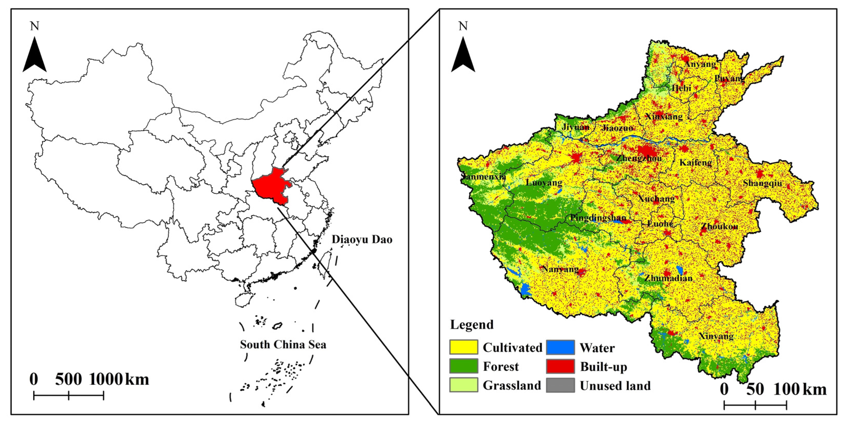
The Henan Province (Figure 1) is in the central region of China, between 31°23′–36°22′N and 110°21′–116°39′E. Its terrain and landforms are diverse and feature extensive vegetation coverage. The province spans the Yangtze, Yellow, Huai, and Hai River basins, with relatively scarce water resources and various types of natural disasters such as drought, floods, pests and diseases, geological disasters, forest fires, and sudden environmental events. In recent years, the number of geological disasters has significantly increased (766 in 2021) and the number of natural disasters, such as forest fires and sudden environmental events, has also remained high. The urbanization rate in the research area has increased annually since 2013, reaching 50% in 2017. The built-up area has been increasing annually, reaching 3235 km2 in 2021. Urbanization has caused a series of environmental problems, such as ecological damage, resource scarcity, and air pollution, which must be better managed and resolved.
2.2. Research Technical Route
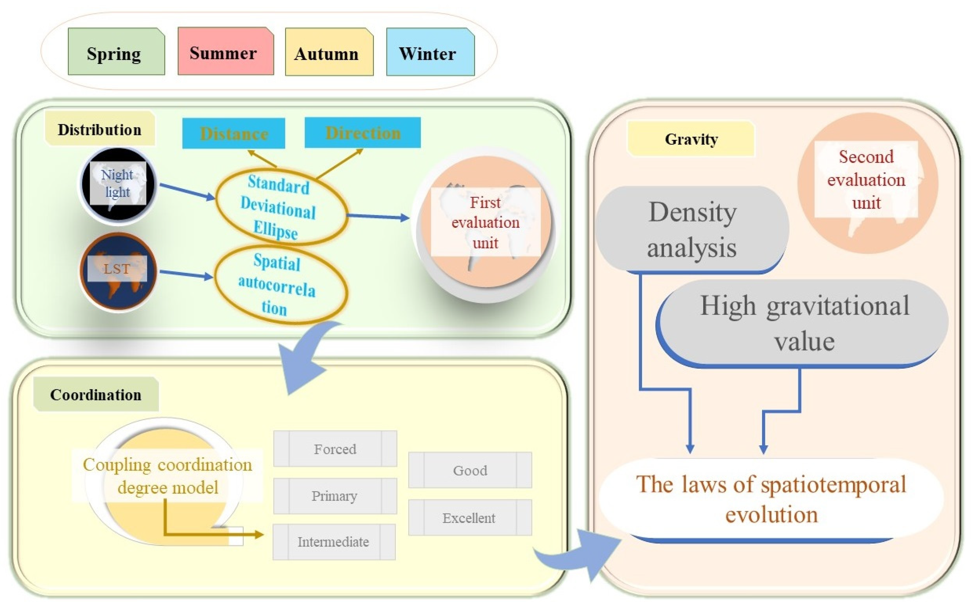
In this study, daily nighttime lighting and the LST were considered the main data sources. The standard deviation ellipses, autocorrelation analysis, coupled coordination models, and gravity models were analyzed. Taking the years 2013, 2016, 2019, and 2022 in the Henan Province as examples, this study delves into the evolutionary laws of LST and gravity. The data were mainly divided based on the 24 solar terms of spring, summer, autumn, and winter and the average method was used for data synthesis to obtain night light data and LST for the four seasons. The natural breakpoint classification method was utilized to consider the high brightness value as the first evaluation unit. The LST in the evaluation unit was extracted. The coupling coordination degree model was used to obtain the coupling coordination relationship between the brightness value and LST; the coordination degree was used as the division scale to obtain the second evaluation unit. Finally, the gravity model was used to explore the space–time evolutionary law of the high gravity area of LST in the second evaluation unit. Figure 2 shows the research technology roadmap, which displays the analysis–coordination–gravity architecture. The main idea of this architecture is to grasp the spatial distribution of the main research content in the region and use the coupling coordination relationship as a transitional process. The coordination part of the coupling coordination relationship can be represented as a “1 + 1 > 2” relationship. In this study, the LST area with high brightness values included concentrated and intense high temperatures. By conducting relevant research on LST and gravity, the spatiotemporal evolution law of LST and gravity was further elucidated.
3. Research Methods and Data
3.1. Standard Deviation Ellipse
The standard deviation ellipse is a method in which graphics are used as representations to depict the spatial variations of elements using parameters such as the area, center of gravity, major and minor axes, and rotation angles of the ellipse. Recently, it has been widely applied in disciplines such as ecology [29], geography [30], and environmental sciences [31]. The equations are as follows:
3.2. Autocorrelation Analysis
The spatial autocorrelation method mainly explores whether variables have spatial dependence or aggregation in space [32,33]. It is mainly divided into global spatial autocorrelation and local spatial autocorrelation [34,35,36] and is generally represented by Moran’s I.
where is the number of samples, is the variance of the kernel density value, and represent the values of the variables in the sample, and is the spatial weight matrix. The range of values for Moran’s I is [–1, 1]. Values greater than 0 indicate positive autocorrelation, values less than 0 indicate negative autocorrelation, and values equal to 0 indicate a random distribution. Furthermore, local spatial autocorrelation was combined to explore the spatial aggregation of the LST with high brightness values.
3.3. Coupling Coordination Model
The coupling coordination degree model integrates the coupling degree and coordination degree indicators [37,38], thereby describing the interaction and coordination level between nighttime light brightness values and the LST. In this study, the focus was placed on variable coordination and then extracted gravitational values. The equations for the coupling coordination degree are:
where , , represent coupling co-scheduling, coordination degree, and coupling degree, respectively; and represent nighttime light brightness values and LST values, respectively; and and are undetermined coefficients that characterize the importance of the variables. In this study, .
3.4. Gravity Model
The basic concept of the gravity model is derived from Newton’s law of universal gravitation [39]. In this study, a gravity model was introduced to study LST. Focusing on the coordination region, the product of the LST of the two regions was divided by the regional distance to reflect the gravitational relationship of the LST. When the gravitational value is larger, the gravitational relationship between the LST between regions is stronger. The equation is as follows:
where is the gravitational value of the LST between regions and ; and represent the LST values between regions and , respectively; is a coefficient, generally 1; is the distance between the center positions of regions and .
3.5. Data Sources and Preprocessing
The nighttime lighting and LST data in this study were obtained from NASA’s Earthdata database (https://www.earthdata.nasa.gov/) and AI Earth (https://engine-aiearth.aliyun.com/). The nighttime lighting data are VNP46A2 data, which include substantial improvements in temporal resolution, calibration, and spatial resolution compared with DMSP-OLS. In this study, a stable light source corrected using the DNB BRDF was extracted. The daily LST data used were MOD11A1. To maintain consistency with the nighttime lighting time, we chose the nighttime LST as the main research object and did not consider daytime LST. The LST was converted into a numerical value in degrees Celsius. The LST and nighttime lighting data were preprocessed through embedding, cropping, and a unified coordinate system. The LST has a resolution of 1 km, and the nighttime lighting data has a resolution of 500 m.
4. Spatiotemporal Gravitational Evolution of the Land Surface Temperature
4.1. Spatiotemporal Distribution of Nighttime Lighting
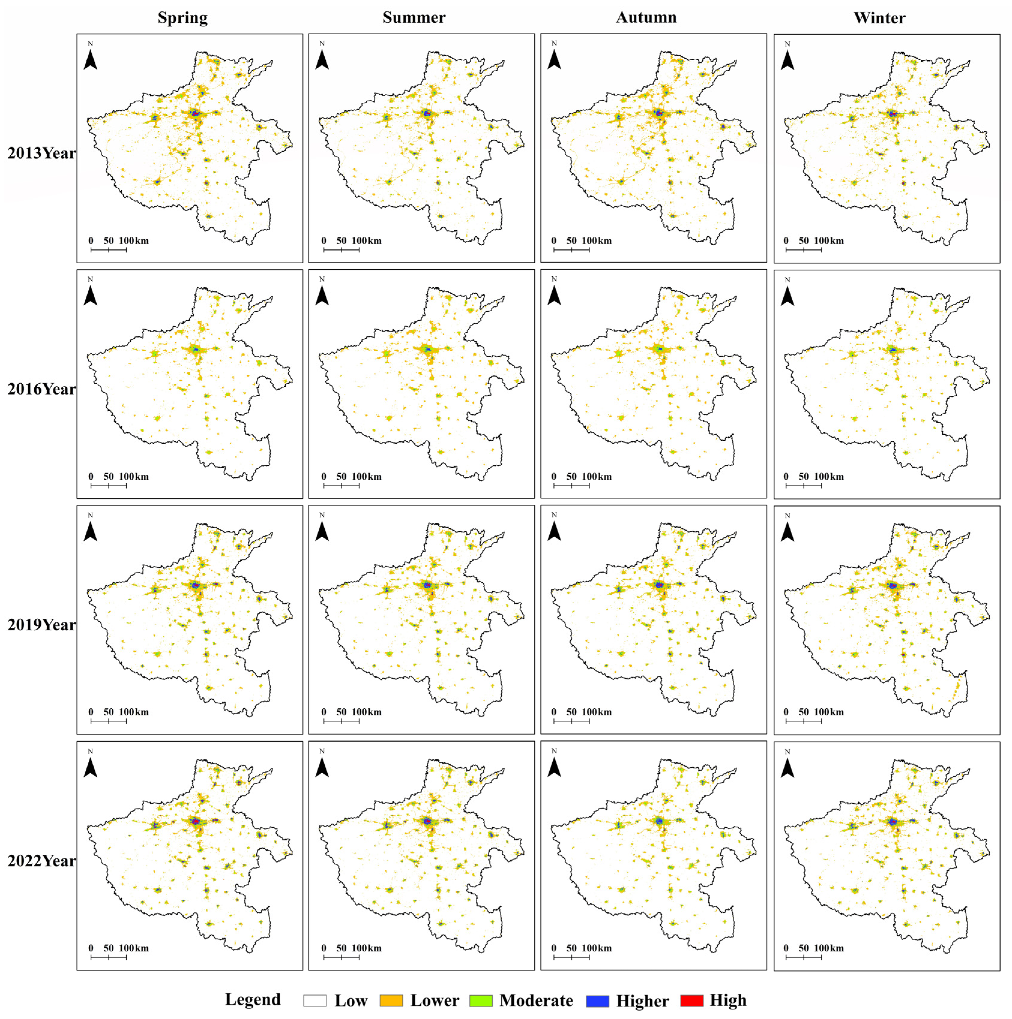
To make reasonable use of the coupling coordination model, spatiotemporal distribution differences in the nighttime lighting brightness values were analyzed (Figure 3). In addition to areas other than those with low nighttime brightness values, the nighttime light was centered around Zhengzhou City and distributed to other prefecture-level cities and counties in the Henan Province. In addition, the nighttime brightness values of cities, such as Pingdingshan, Jiaozuo, Xuchang, and Xinxiang, were high. The nighttime light brightness had a large distribution area in 2013, 2019, and 2022 and the nighttime light in 2013 and 2019 showed a balanced distribution throughout the four seasons, without significant differences. The nighttime lighting brightness was weaker in 2016, especially in autumn and winter. The nighttime lighting brightness in autumn 2022 was slightly weak and gradually increased in winter.
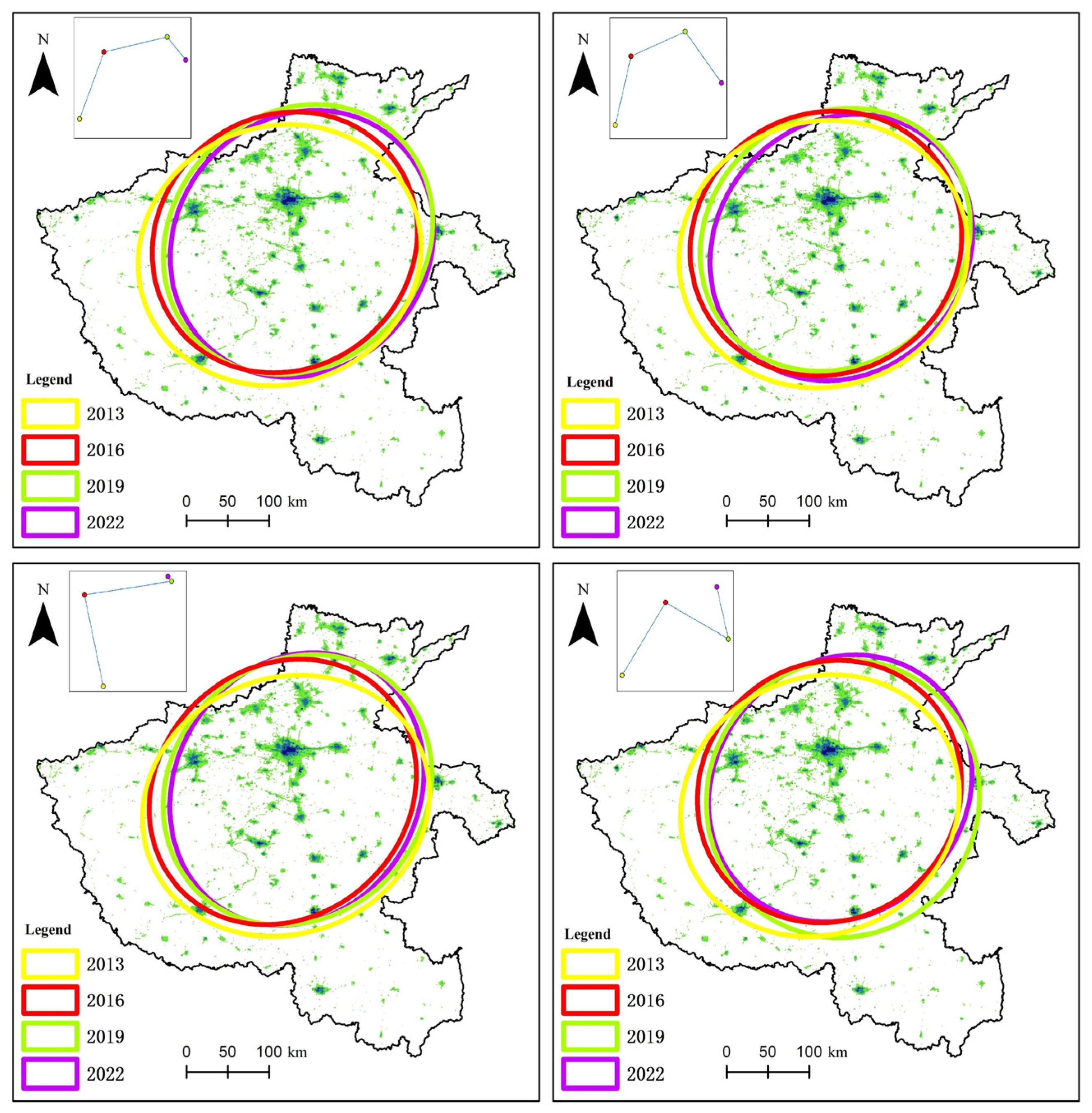
In this study, areas other than those with low light intensity were selected as the first evaluation unit, and the directional distribution of the first evaluation unit was explored using a standard deviation ellipse (Figure 4; the scale of the thumbnail in the upper left corner is inconsistent). Table 1 shows the offset distances of the standard deviation ellipses for the three time periods in the study area, which indirectly indicate the magnitude of nighttime lighting offset. In the first two periods of spring, the offset distance was similar and the offset amplitude was consistent, whereas the offset amplitude significantly decreased in the last period. The shift amplitude in summer was relatively small in the three time periods, with a slightly larger shift amplitude in the first period. The amplitude in the first two periods of autumn was consistent, but a sharp decrease in the shift amplitude occurred in the third period, indicating that the change in the lighting brightness during the autumn period was relatively small. The deviation amplitude in winter decreased from the first to the third period. Overall, the deviation distance and amplitude exhibited significant changes in the first period, whereas the changes in the last period were relatively small. This indicates that the social, economic, and demographic changes in the Henan Province have been relatively small in the past four years compared with those in 2013 and 2016.
In spring, the first evaluation unit shifted toward the eastern region, and the direction of the shift in summer was similar to that in spring. The shift direction in autumn changed, shifting from the northeast direction in spring and summer to the northwest direction from 2013 to 2016, and the shift direction also changed from 2019 to 2022. The winter shift direction returned to the same direction as in spring and summer in the 2013–2016 period, shifted southeast in the 2016–2019 time period, and shifted in the same direction as in autumn in the 2019–2022 time period.
4.2. Spatiotemporal Correlation Characteristics of the Land Surface Temperature
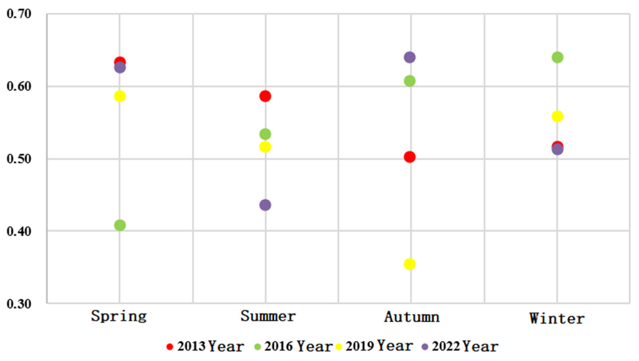
Figure 5 shows the global spatial autocorrelation results. The autocorrelation test for LST under the first evaluation unit in all years yielded Z > 2.58, with a p-value below 0.01 and a positive Moran’s I. This indicates that LST was not randomly distributed and showed a positive autocorrelation at the 99.9% confidence level. The LST trend was the same, and a spatial clustering effect was observed. In 2013 and 2019, Moran’s I first decreased and then increased with seasonal changes, indicating that the aggregation degree of the LST also first decreased and then increased. The degree of aggregation in 2016 gradually increased with the change in seasons and the degree of aggregation in 2022 showed an oscillating evolution pattern. From a seasonal perspective, the degree of LST aggregation in the spring of 2016 was lower than that of the other three years. The degree of LST aggregation in the summer of 2016 surpassed that of 2019 and 2022 and the degree of aggregation in 2013 remained in a leading position. The degree of aggregation in autumn decreased significantly in 2019, with 2022 having the highest degree of aggregation. The Moran’s I values in winter were all greater than 0.5. The year 2016 showed the highest degree of clustering, whereas the other three years had similar degrees of clustering.
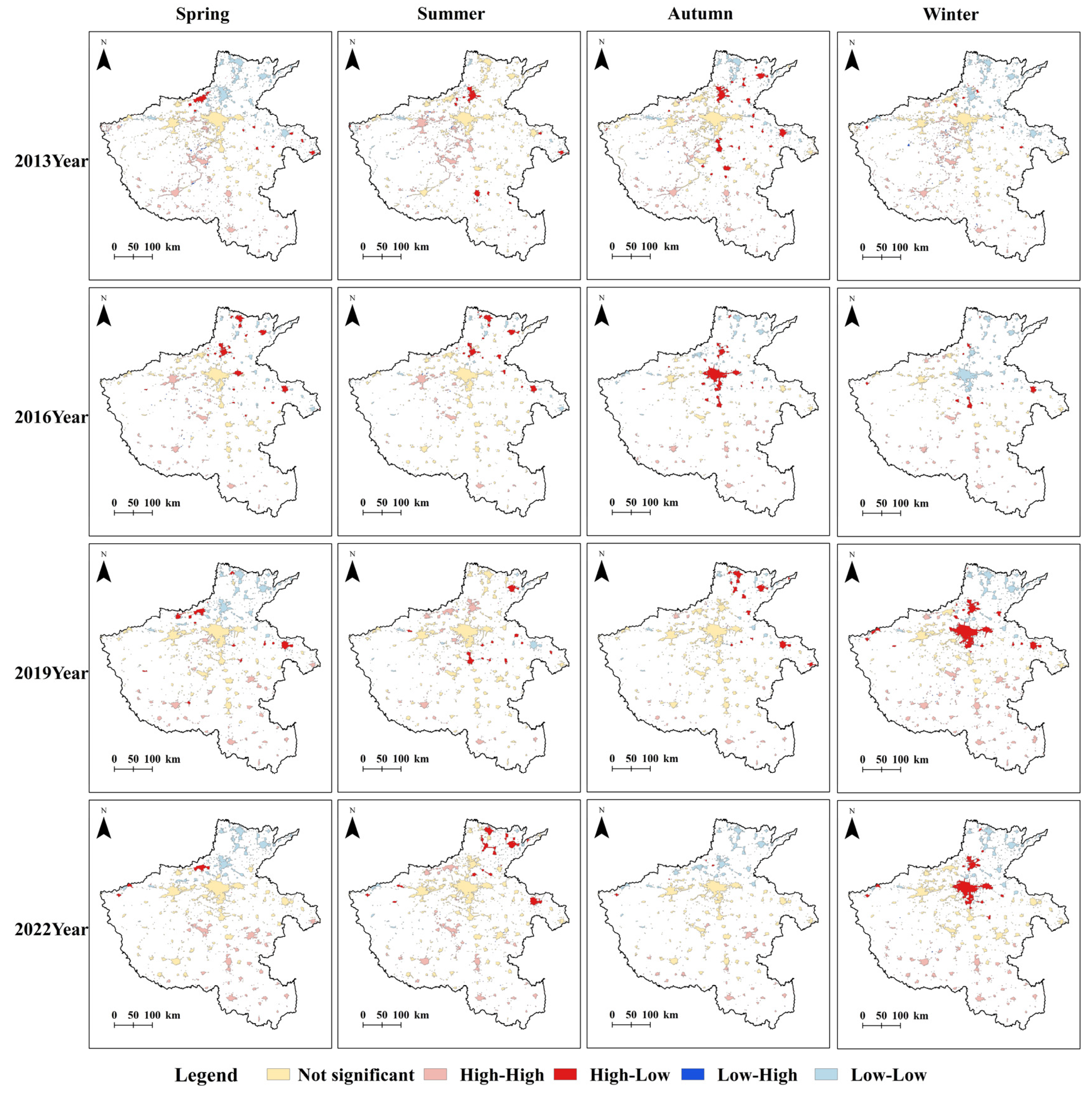
To analyze the spatial aggregation and diffusion of the LST more intuitively, a local autocorrelation test was conducted. Figure 6 shows the results. In 2013, the high–high aggregates in spring, autumn, and winter were mainly concentrated in the southern part of the Henan Province, whereas they were mainly concentrated in the central region in summer. The high–low aggregates were scattered in small amounts throughout the Henan Province, with large areas appearing in summer and autumn. In 2016, The high–high aggregates were mainly located in the southern region of the study area, with significant differences in the degree of aggregation between the spring and summer and autumn and winter seasons. In spring and summer, more high–low aggregates were observed in the southern region, which transformed into low–low aggregates during autumn and winter. Large areas around Zhengzhou City also transitioned from insignificant clustering to high–low and low–low aggregates in spring and summer, respectively. In spring and winter of 2019, the clustering types in the southern region of the study area were similar to those in the northern region. Except for the low–high clustering types in summer, the clustering types were evenly distributed throughout the study area, whereas the insignificant ones in autumn occupied most of the area, with some clusters located at the edge of the study area. The cluster distribution in 2022 was similar to that in 2019, with spring and winter being the most similar. In summer, the northern cluster shifted from an insignificant to a high–low cluster, whereas the northern region shifted from a high–low to a low–low cluster in autumn.
4.3. Spatiotemporal Gravity Analysis of the Night Land Surface Temperature
In this study, the coupling coordination model was used to extract the second evaluation unit, and the coupling coordination between nighttime light brightness and LST values was explored. The first evaluation unit of the coordination part was extracted as the second evaluation unit and the LST gravity value of the second evaluation unit was calculated, with the high gravity value as the main focus of the study.
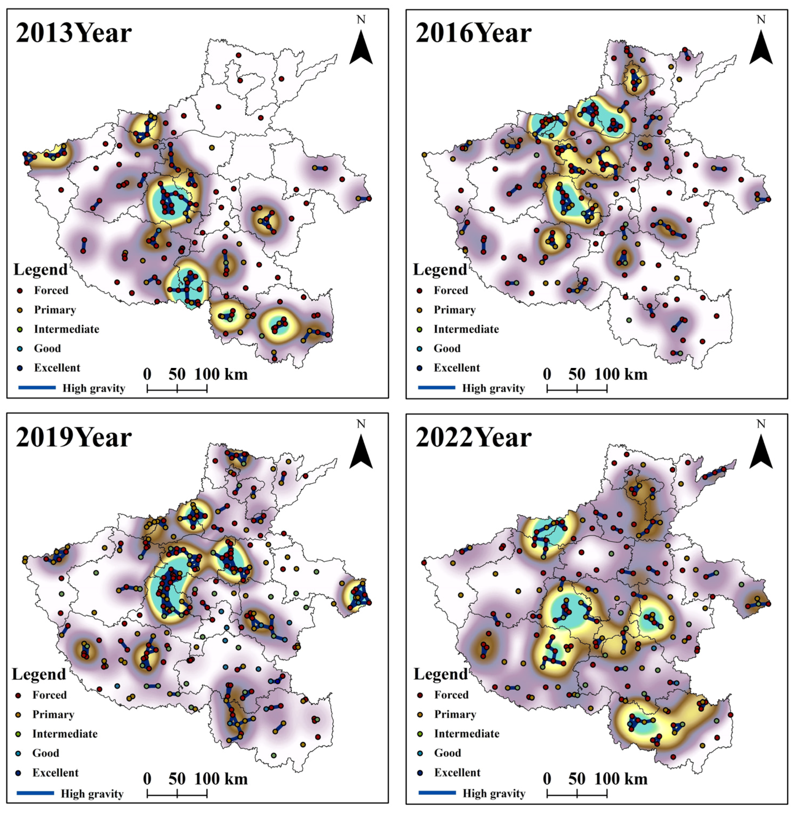
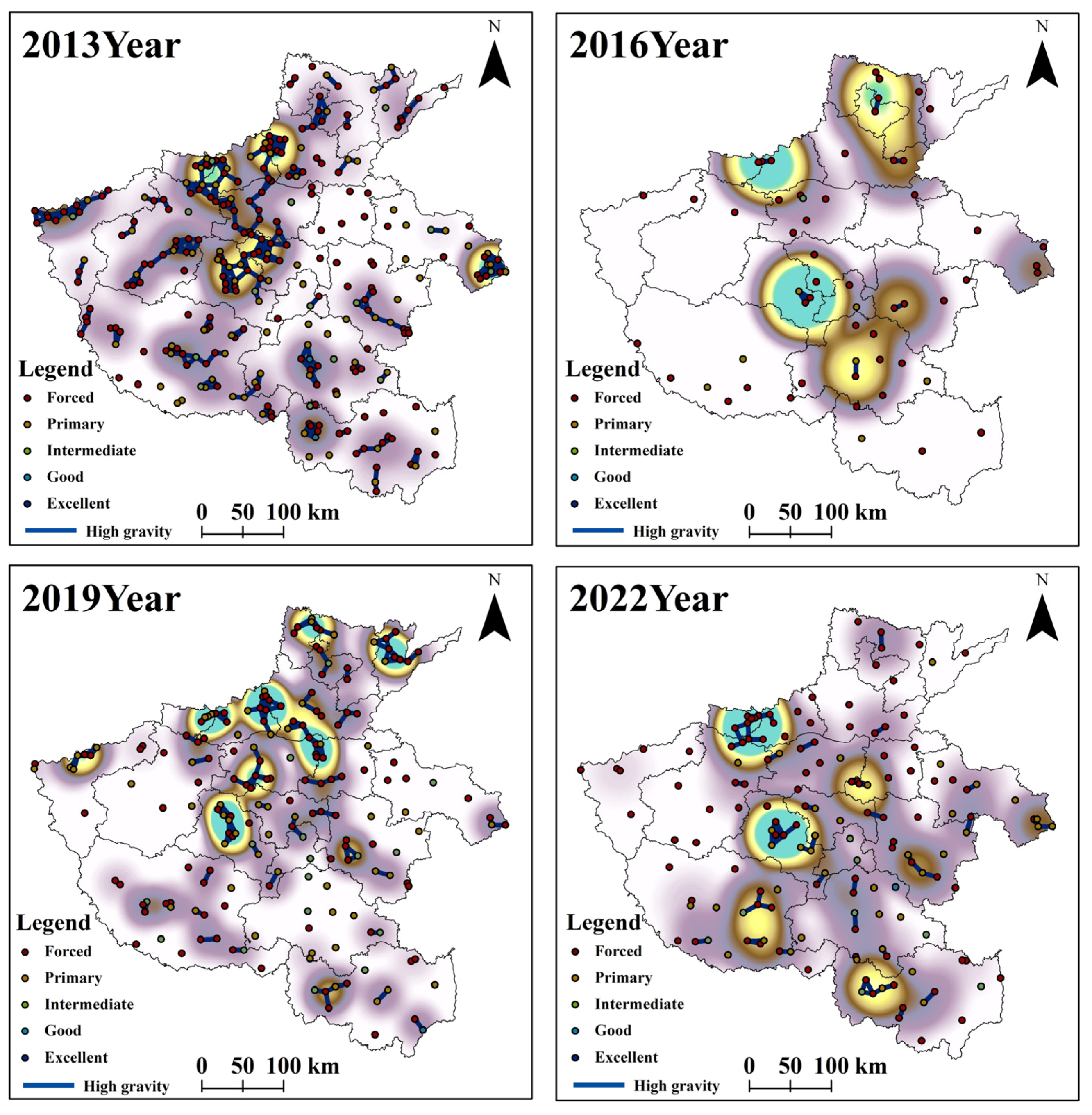
Figure 7 shows the spatiotemporal distribution of the high-gravity LST in spring. The high gravity values in spring showed certain differences in their spatial and temporal dimensions. In 2013, high-gravity values did not appear in the northern region of the Henan Province but were more densely distributed in the western and southern regions, mainly at the junction of Pingdingshan City, Zhumadian and Nanyang City, and Xinyang City. In 2016, high-gravity values gradually shifted to the north and appeared as high-density distributions in Xinxiang, Jiaozuo, Hebi City, and other places. High-gravity value densities in Zhumadian, Nanyang, and Xinyang gradually decreased. The high-gravity values in 2019 were mainly distributed in Pingdingshan, Xinxiang, Jiaozuo, and Kaifeng as well as around Shangqiu City. The distribution of high-gravity values in 2022 was relatively balanced. Except for Luoyang, Sanmenxia, and Zhengzhou, which had lower values, the prefecture-level cities had higher or lower gravity values. The two ends of the springtime nodes were located at extremely high and extremely low temperatures for the entire year’s LST. At the same time, they were in the transitional season of vegetation presence to absence. Such geographical features and climate can lead to differences in the gravity of LST. Except for the significant spatial differences in 2013, high-gravity values in the other years were mostly evenly distributed.
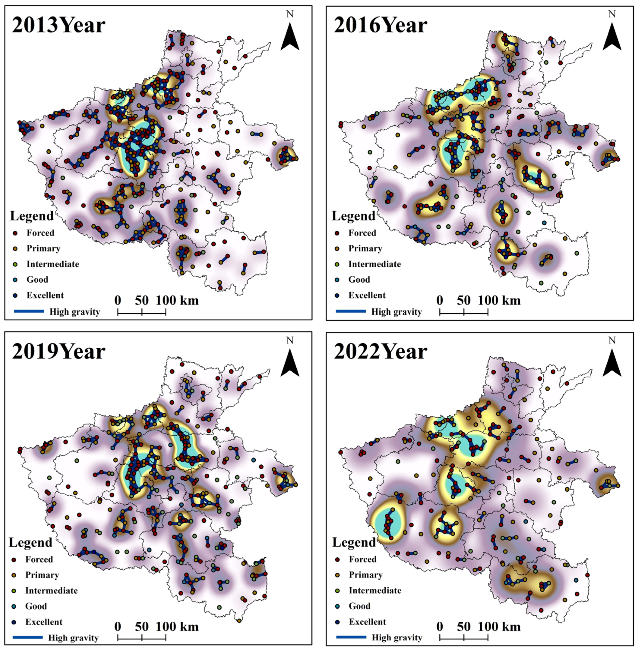
Figure 8 shows the spatiotemporal distribution of the high-gravity LST in summer. The distribution of high-gravity values in summer was denser than that in spring. In 2013, a very high distribution density was observed from Anyang City to the southwest, with the overall distribution in the east being sparser than in the west. The high-gravity value distribution in 2016 was mainly centered around Zhengzhou City, spreading towards cities such as Pingdingshan, Jiaozuo, Xinxiang, and Jiyuan. In addition, small areas with a high-gravity value distribution also appeared in cities such as Zhumadian, Zhoukou, and Shangqiu, and the distribution of high-gravity values was denser in 2019 than in 2016. Zhengzhou and Pingdingshan City had high-gravity values that pulled each other and became dense centers. The distribution of high-gravity values in the northern region of the Henan Province was wider and denser. The distribution of high-gravity values in 2022 was generally sparse compared with other years, with an increase in high-gravity values in the southern region. Summer is the hottest season of the year and the LST reached its highest value at night. The distribution density of high-gravity values showed a clear upward trend. In addition, because of prolonged sunlight and strong solar radiation, the distribution density of high-gravity values was more prominent in areas with dense human activity. However, over the years, the distribution density of high-gravity values decreased, which may be related to the deep governance of the ecological environment by the local government.
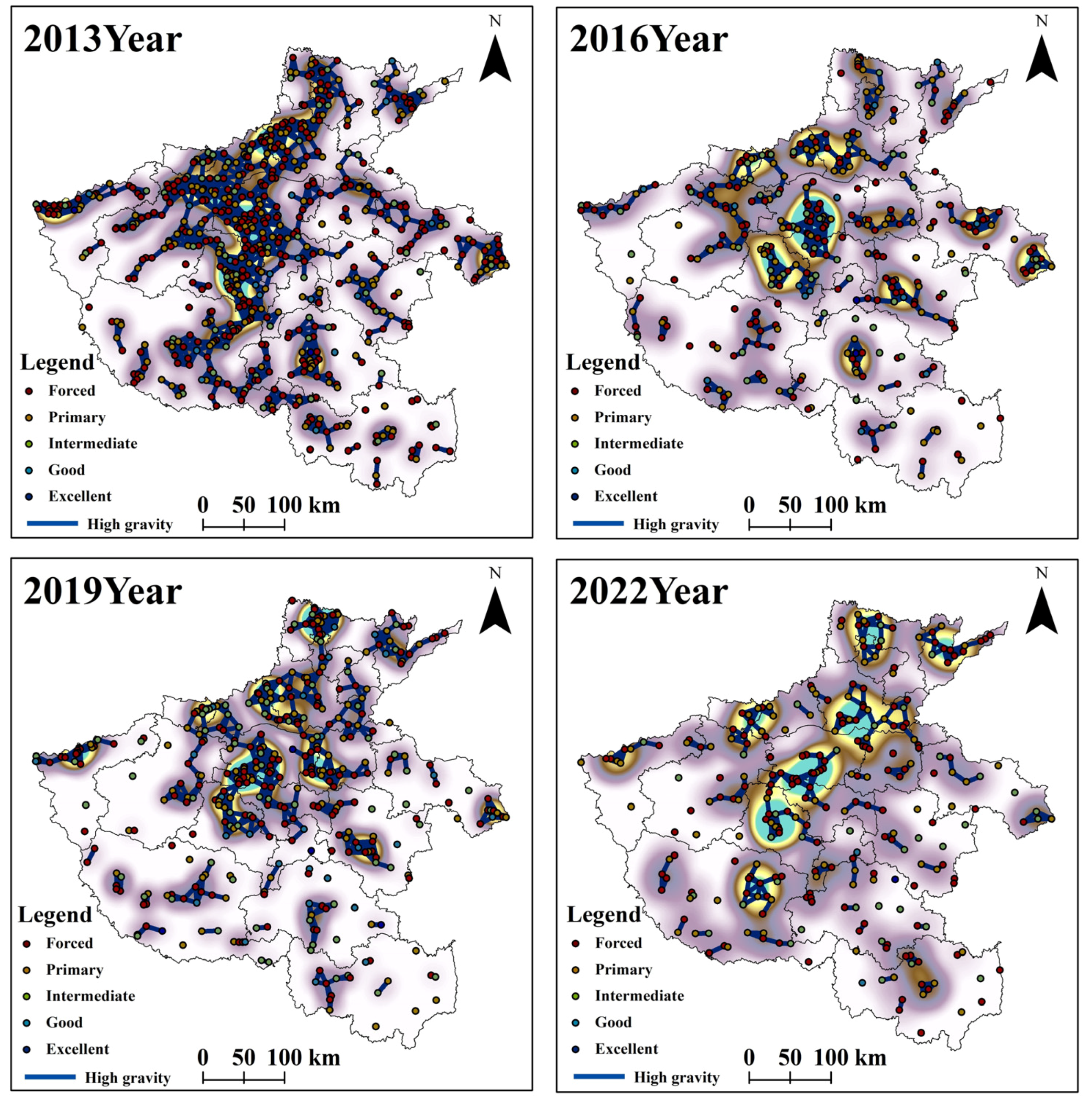
Figure 9 shows the spatiotemporal distribution of the high-gravity LST in autumn. Compared with summer, the density distribution of high-gravity values decreased significantly in autumn. In 2013, the primary core distribution in Zhengzhou disappeared. High-gravity values were mainly observed in Xinxiang, Jiyuan, Jiaozuo, Shangqiu, Pingdingshan, and other cities. Notably, the high-density distribution of high-gravity values also appeared in the western region of Sanmenxia City. In 2016, the distribution of high-gravity values was the lowest, appearing only sporadically in some areas of cities such as Anyang, Jiyuan, Jiaozuo, Pingdingshan, and Luohe. In 2019, the distribution of high-gravity values gradually recovered. Simultaneously, the high-gravity density centered around Zhengzhou City reappeared, and many high-gravity values were distributed in the northern region of the Henan Province. The high-gravity value distribution density in 2022 shifted towards sparsity and presented a uniform distribution. The nighttime LST showed a downward trend in autumn, which was much lower than the high-temperature heat waves in summer. The solar radiation and sunlight were significantly reduced and the distribution of high-gravity values of LST decreased, especially in late autumn at the transition to winter. The significant decrease in the nighttime LST also affected the overall high-gravity distribution of the LST in autumn.
Figure 10 shows the spatiotemporal distribution of the high-gravity LST in winter. The distribution of high-gravity values in winter was denser than that of spring and autumn. In 2013, high-density values were mainly distributed at the junction of Pingdingshan, Xuchang, and Zhengzhou City, whereas other high-gravity values were scattered in the Henan Province. The distribution of high-gravity values in 2016 and 2019 was relatively similar and evenly distributed in the study area. The high-gravity densities of Pingdingshan, Xuchang, Zhengzhou, and other cities maintained their peak values. Although the distribution of high-gravity values in 2022 was relatively uniform, the distribution of high-gravity values gradually became discrete. Due to the relatively low impact of clouds and air humidity on winter solar radiation, the LST decreased. In addition to factors such as sunlight and solar radiation, weather changes, such as snowfall and frost, were also observed. Although the distribution density of the high-gravity values was high, the overall gravity value was low, which was closely related to the overall decrease in the LST.
According to the above results and analysis, the spatiotemporal gravity distribution of LST showed very large differences, and the spatiotemporal gravity distribution at most time nodes demonstrated an aggregation distribution. From the temporal perspective, combined with the evolutionary direction of night light, we know that with the continuous acceleration of urbanization in Henan Province from 2013 to 2022, great changes in population, economy, and environment [40] will inevitably lead to changes in the gravity of LST. From the seasonal perspective, the difference between the four seasons is not only an alternate evolution to that of time. The transition of the seasons causes certain changes in vegetation, water, animal activities, and ecology [41], which also affect LST.
5. Discussion and Conclusions
5.1. Discussion
In this study, daily nighttime lighting and LST data and seasonal data were selected and fused according to the division of the four seasons into 24 solar terms, completing in-depth data mining. In this study, we proposed and applied the suitable analysis–coordination–gravity research framework. We fused the daily data to make relevant research on LST accurate at the daily scale, which has practical and theoretical significance. The LST is an important parameter in ecological processes such as climate [42], environment [43,44], resource management [45], and urban construction [46,47], and is closely related to humans. A reasonable analysis of the spatiotemporal evolution of LST gravity can facilitate the sustainable development of the ecological environment. In addition, the focus of this research was placed on high-gravity changes in the LST in areas with high nighttime lighting brightness values. These areas have a significant effect on high-temperature heat waves in cities and rural areas. Studying their seasonal evolution can provide guidance to better control the LST as well as develop ideas for research on the heat island effect and thermal environment.
In this study, only the spatiotemporal gravity law of the nighttime LST was discussed, and factors influencing of the LST spatiotemporal gravity were not considered. However, these factors can be used to analyze the urban heat island effect, which has a significant effect on species distribution, ecological adaptation, and climate change. In addition, the gravity mining of LST is not deep enough. Due to the limited scope of this study, the gravity of LST in each year is not explored, which may lead to the neglect of some evolutionary laws. In future research, we aim to determine the factors affecting the LST gravity and pay more attention to the study of longer time series, so as to provide guidance for government decision-making, resource management and environmental management.
5.2. Conclusions
In this study, we utilized daily LST and nighttime light data in combination with the analysis–coordination–gravity research framework to explore the spatiotemporal and gravitational evolutionary laws of the LST in the Henan Province in 2013, 2016, 2019, and 2022. We focused on areas with high brightness values that had high coupling and coordination with the LST. The high-temperature heat waves generated in this area were particularly severe. The results can be summarized as follows:
- (1)
- The high brightness values of nighttime lights had a larger distribution area in 2013, 2019, and 2022, with a larger deviation in the winter of 2013–2016 and a smaller deviation in the autumn of 2019–2022. The deviation direction also significantly varied in different seasons, except for spring and summer.
- (2)
- The distribution of the LST under the first evaluation unit was not randomized and presented a positive autocorrelation with a 99.9% confidence interval. Moran’s I values in winter were greater than 0.5. The local spatial autocorrelation results indicate that clustering was mainly distributed at the northern and southern ends of the Henan Province. Close to the more developed Zhengzhou City, only four nodes showed a clustering distribution.
- (3)
- The distribution of high-gravity values showed a differentiated pattern across different years and seasons. Because of seasonal differences, the LST is influenced by multiple factors such as solar radiation, sunlight, and rainfall. The distribution of high-gravity values was relatively dense in summer, whereas in the milder seasons of spring and autumn it showed a uniform distribution in most years. The distribution in winter appeared to be denser than that in spring and autumn; however, the overall gravity value was relatively low.
In addition to the connection of population, policy and economy among regions, the correlation between thermal environment and LST cannot be ignored. To control the harm caused by the heat island effect at the provincial level, further consideration of the evolutionary process of LST across seasons and time is necessary. In addition to its own heat, the attraction among LST must be considered. These research results are of great significance for a deeper understanding of the relationship between nighttime brightness changes and the LST and provide a scientific basis and decision-making support for urban planning and environmental management.
Author Contributions
Conceptualization, Q.F. and Y.S.; Data curation, Y.S.; Investigation, B.M. and Y.S.; Methodology, Q.F. and N.C.; Validation, Y.S. and B.M.; Visualization, Y.S.; Writing—original draft, Q.F. and Y.S.; Writing—review and editing, Q.F., Y.S., N.C., and B.M. All authors have read and agreed to the published version of the manuscript.
Funding
This research was funded by the Project supported by discipline innovation team of Liaoning Technical University (grant number LNTU20TD-06).
Data Availability Statement
Please refer to Chapter 3.5 of the article for detailed information on the sources of data used in this study.
Conflicts of Interest
The authors declare no conflict of interest.
References
- Waltham, N.J.; Elliott, M.; Lee, S.Y.; Lovelock, C.; Duarte, C.M.; Buelow, C.; Simenstad, C.; Nagelkerken, I.; Claassens, L.; Wen, C.K.C.; et al. UN decade on ecosystem restoration 2021–2030—What chance for success in restoring coastal ecosystems? Front. Mar. Sci. 2020, 7, 71. [Google Scholar] [CrossRef]
- Aronson, J.; Goodwin, N.; Orlando, L.; Eisenberg, C.; Cross, A.T. A world of possibilities: Six restoration strategies to support the United Nation’s Decade on Ecosystem Restoration. Restor. Ecol. 2020, 28, 730–736. [Google Scholar] [CrossRef]
- Xue, B.L.; Wang, L.; Yang, K.; Tian, L.; Qin, J.; Chen, Y.; Zhao, L.; Ma, Y.; Koike, T.; Hu, Z.; et al. Modeling the land surface water and energy cycles of a mesoscale watershed in the central Tibetan Plateau during summer with a distributed hydrological model. J. Geophys. Res. Atmos. 2013, 118, 8857–8868. [Google Scholar] [CrossRef]
- Yang, K.; Wu, H.; Qin, J.; Lin, C.; Tang, W.; Chen, Y. Recent climate changes over the Tibetan Plateau and their impacts on energy and water cycle: A review. Glob. Planet. Change 2014, 112, 79–91. [Google Scholar] [CrossRef]
- Rahaman, Z.A.; Kafy, A.-A.; Saha, M.; Rahim, A.A.; Almulhim, A.I.; Rahaman, S.N.; Fattah, M.A.; Rahman, M.T.; Kalaivani, S.; Al Rakib, A.J.B.; et al. Assessing the impacts of vegetation cover loss on surface temperature, urban heat island and carbon emission in Penang city, Malaysia. Build. Environ. 2022, 222, 109335. [Google Scholar] [CrossRef]
- Ren, J.; Yang, J.; Wu, F.; Sun, W.; Xiao, X.; Xia, J. Regional thermal environment changes: Integration of satellite data and land use/land cover. iScience 2023, 26, 105820. [Google Scholar] [CrossRef]
- Marando, F.; Salvatori, E.; Sebastiani, A.; Fusaro, L.; Manes, F. Regulating ecosystem services and green infrastructure: Assessment of urban heat island effect mitigation in the municipality of Rome, Italy. Ecol. Modell. 2019, 392, 92–102. [Google Scholar] [CrossRef]
- Estoque, R.C.; Ooba, M.; Seposo, X.T.; Togawa, T.; Hijioka, Y.; Takahashi, K.; Nakamura, S. Heat health risk assessment in Philippine cities using remotely sensed data and social-ecological indicators. Nat. Commun. 2020, 11, 1581. [Google Scholar] [CrossRef]
- Bastos, A.; Ciais, P.; Friedlingstein, P.; Sitch, S.; Pongratz, J.; Fan, L.; Wigneron, J.-P.; Weber, U.; Reichstein, M.; Fu, Z.; et al. Direct and seasonal legacy effects of the 2018 heat wave and drought on European ecosystem productivity. Sci. Adv. 2020, 6, eaba2724. [Google Scholar] [CrossRef]
- Yang, J.; Xin, J.; Zhang, Y.; Xiao, X.; Xia, J.C. Contributions of sea–land breeze and local climate zones to daytime and nighttime heat island intensity. Npj Urban. Sustain. 2022, 2, 12. [Google Scholar] [CrossRef]
- Feng, S.; Lu, H.; Tian, P.; Xue, Y.; Lu, J.; Tang, M.; Feng, W. Analysis of microplastics in a remote region of the Tibetan Plateau: Implications for natural environmental response to human activities. Sci. Total. Environ. 2020, 739, 140087. [Google Scholar] [CrossRef]
- Gibson, J.; Olivia, S.; Boe-Gibson, G.; Li, C. Which night lights data should we use in economics, and where? J. Dev. Econ. 2021, 149, 102602. [Google Scholar] [CrossRef]
- Stathakis, D.; Baltas, P. Seasonal population estimates based on night-time lights. Comput. Environ. Urban Syst. 2018, 68, 133–141. [Google Scholar] [CrossRef]
- You, H.; Yang, J.; Xue, B.; Xiao, X.; Xia, J.; Jin, C.; Li, X. Spatial evolution of population change in Northeast China during 1992–2018. Sci. Total Environ. 2021, 776, 146023. [Google Scholar] [CrossRef]
- Bhattarai, D.; Lucieer, A.; Lovell, H.; Aryal, J. Remote sensing of night-time lights and electricity consumption: A systematic literature review and meta-analysis. Geogr. Compass. 2023, 17, e12684. [Google Scholar] [CrossRef]
- Li, L.; Yu, T.; Zhao, L.; Zhan, Y.; Zheng, F.; Zhang, Y.; Mumtaz, F.; Wang, C. Characteristics and trend analysis of the relationship between land surface temperature and nighttime light intensity levels over China. Infrared Phys. Technol. 2019, 97, 381–390. [Google Scholar] [CrossRef]
- Guo, A.; Yang, J.; Sun, W.; Xiao, X.; Cecilia, J.X.; Jin, C.; Li, X. Impact of urban morphology and landscape characteristics on spatiotemporal heterogeneity of land surface temperature. Sustain. Cities Soc. 2020, 63, 102443. [Google Scholar] [CrossRef]
- Liang, Z.; Wu, S.; Wang, Y.; Wei, F.; Huang, J.; Shen, J.; Li, S. The relationship between urban form and heat island intensity along the urban development gradients. Sci. Total Environ. 2020, 708, 135011. [Google Scholar] [CrossRef]
- Levin, N.; Kyba, C.C.; Zhang, Q.; de Miguel, A.S.; Román, M.O.; Li, X.; Portnov, B.A.; Molthan, A.L.; Jechow, A.; Miller, S.D.; et al. Remote sensing of night lights: A review and an outlook for the future. Remote Sens. Environ. 2020, 237, 111443. [Google Scholar] [CrossRef]
- Levin, N.; Kark, S.; Crandall, D. Where have all the people gone? Enhancing global conservation using night lights and social media. Ecol. Appl. 2015, 25, 2153–2167. [Google Scholar] [CrossRef]
- Stokes, E.C.; Seto, K.C. Characterizing urban infrastructural transitions for the Sustainable Development Goals using multi-temporal land, population, and nighttime light data. Remote Sens. Environ. 2019, 234, 111430. [Google Scholar] [CrossRef]
- Liu, S.; Shi, K.; Wu, Y.; Chang, Z. Remotely sensed nighttime lights reveal China’s urbanization process restricted by haze pollution. Build. Environ. 2021, 206, 108350. [Google Scholar] [CrossRef]
- Kabir, M.; Salim, R.; Al-Mawali, N. The gravity model and trade flows: Recent developments in econometric modeling and empirical evidence. Econ. Anal. Policy 2017, 56, 60–71. [Google Scholar] [CrossRef]
- Balogh, J.M.; Aguiar, G.M.B. Determinants of Latin American and the Caribbean agricultural trade: A gravity model approach. Agric. Econ. 2022, 68, 127–136. [Google Scholar] [CrossRef]
- Kuik, O.; Branger, F.; Quirion, P. Competitive advantage in the renewable energy industry: Evidence from a gravity model. Renew. Energry 2019, 131, 472–481. [Google Scholar] [CrossRef]
- Li, Q.; Zhou, Y.; Yi, S. An integrated approach to constructing ecological security patterns and identifying ecological restoration and protection areas: A case study of Jingmen, China. Ecol. Indic. 2022, 137, 108723. [Google Scholar] [CrossRef]
- Qu, H.; Yin, Y.; Li, J.; Xing, W.; Wang, W.; Zhou, C.; Hang, Y. Spatio-temporal Evolution of the Agricultural Eco-efficiency Network and Its Multidimensional Proximity Analysis in China. Chin. Geogr. Sci. 2022, 32, 724–744. [Google Scholar] [CrossRef]
- Xiao, S.; Wu, W.; Guo, J.; Ou, M.; Pueppke, S.G.; Ou, W.; Tao, Y. An evaluation framework for designing ecological security patterns and prioritizing ecological corridors: Application in Jiangsu Province, China. Landsc. Ecol. 2020, 35, 2517–2534. [Google Scholar] [CrossRef]
- Zhang, L.; Hu, B.; Zhang, Z.; Liang, G. Research on the spatiotemporal evolution and mechanism of ecosystem service value in the mountain-river-sea transition zone based on “production-living-ecological space”—Taking the Karst-Beibu Gulf in Southwest Guangxi, China as an example. Ecol. Indic. 2023, 148, 109889. [Google Scholar] [CrossRef]
- Qiao, K.; Zhu, W.; Hu, D.; Hao, M.; Chen, S.; Cao, S. Examining the distribution and dynamics of impervious surface in different function zones in Beijing. J. Geogr. Sci. 2018, 28, 669–684. [Google Scholar] [CrossRef]
- Hu, J.; Liang, J.; Fang, J.; He, H.; Chen, F. How do industrial land price and environmental regulations affect spatiotemporal variations of pollution-intensive industries? Regional analysis in China. J. Clean. Prod. 2022, 333, 130035. [Google Scholar] [CrossRef]
- Xiao, G.; Hu, Y.; Li, N.; Yang, D. Spatial autocorrelation analysis of monitoring data of heavy metals in rice in China. Food Control. 2018, 89, 32–37. [Google Scholar] [CrossRef]
- Liu, Q.; Wang, S.; Zhang, W.; Zhan, D.; Li, J. Does foreign direct investment affect environmental pollution in China’s cities? A spatial econometric perspective. Sci. Total. Environ. 2018, 613, 521–529. [Google Scholar] [CrossRef] [PubMed]
- Wang, S. Spatial patterns and social-economic influential factors of population aging: A global assessment from 1990 to 2010. Soc. Sci. Med. 2020, 253, 112963. [Google Scholar] [CrossRef]
- Ren, H.; Shang, Y.; Zhang, S. Measuring the spatiotemporal variations of vegetation net primary productivity in Inner Mongolia using spatial autocorrelation. Ecol. Indic. 2020, 112, 106108. [Google Scholar] [CrossRef]
- Yan, D.; Lei, Y.; Shi, Y.; Zhu, Q.; Li, L.; Zhang, Z. Evolution of the spatiotemporal pattern of PM2.5 concentrations in China–A case study from the Beijing-Tianjin-Hebei region. Atmos. Environ. 2018, 183, 225–233. [Google Scholar] [CrossRef]
- Xing, L.; Xue, M.; Hu, M. Dynamic simulation and assessment of the coupling coordination degree of the economy–resource–environment system: Case of Wuhan City in China. J. Environ. Manag. 2019, 230, 474–487. [Google Scholar] [CrossRef]
- Shi, T.; Yang, S.; Zhang, W.; Zhou, Q. Coupling coordination degree measurement and spatiotemporal heterogeneity between economic development and ecological environment----Empirical evidence from tropical and subtropical regions of China. J. Clean. Prod. 2020, 244, 118739. [Google Scholar] [CrossRef]
- Bruno, G.; Improta, G. Using gravity models for the evaluation of new university site locations: A case study. Comput. Oper. Res. 2008, 35, 436–444. [Google Scholar] [CrossRef]
- Liu, Y.; Li, J.; Yang, Y. Strategic adjustment of land use policy under the economic transformation. Land Use Policy 2018, 74, 5–14. [Google Scholar] [CrossRef]
- Bastian, M.; Hawitt, R.B. Multi-species, ecological and climate change temporalities: Opening a dialogue with phenology. Environ. Plan E Nat. Space 2023, 6, 1074–1097. [Google Scholar] [CrossRef]
- Chen, Y.; Yang, J.; Yu, W.; Ren, J.; Xiao, X.; Xia, J.C. Relationship between urban spatial form and seasonal land surface temperature under different grid scales. Sustain. Cities Soc. 2023, 89, 104374. [Google Scholar] [CrossRef]
- Ren, J.; Yang, J.; Zhang, Y.; Xiao, X.; Xia, J.C.; Li, X.; Wang, S. Exploring thermal comfort of urban buildings based on local climate zones. J. Clean. Prod. 2022, 340, 130744. [Google Scholar] [CrossRef]
- Yang, J.; Yang, Y.; Sun, D.; Jin, C.; Xiao, X. Influence of urban morphological characteristics on thermal environment. Sustain. Cities Soc. 2021, 72, 103045. [Google Scholar] [CrossRef]
- Luo, X.; Yang, J.; Sun, W.; He, B. Suitability of human settlements in mountainous areas from the perspective of ventilation: A case study of the main urban area of Chongqing. J. Clean. Prod. 2021, 310, 127467. [Google Scholar] [CrossRef]
- Chen, Y.; Yang, J.; Yang, R.; Xiao, X.; Xia, J. Contribution of urban functional zones to the spatial distribution of urban thermal environment. Build. Environ. 2022, 216, 109000. [Google Scholar] [CrossRef]
- Xie, P.; Yang, J.; Sun, W.; Xiao, X.; Xia, J. Urban scale ventilation analysis based on neighborhood normalized current model. Sustain. Cities Soc. 2022, 80, 103746. [Google Scholar] [CrossRef]
Figure 1.
Map showing the location of the study area.

Figure 2.
Research roadmap.

Figure 3.
Spatiotemporal distribution of luminance values of night lights.

Figure 4.
Direction map of light evolution at night.

Figure 5.
Evolution of global Moran’s I (Z > 2.58; p < 0.01).

Figure 6.
Spatial distribution of local Moran’s I.

Figure 7.
Spatiotemporal distribution of the high-gravity land surface temperature in spring.

Figure 8.
Spatiotemporal distribution of the high-gravity land surface temperature in summer.

Figure 9.
Spatiotemporal distribution of the high-gravity land surface temperature in autumn.

Figure 10.
Spatiotemporal distribution of the high-gravity land surface temperature in winter.


Table 1.
Deviation of the standard deviation ellipse.
| Distance/m | 2013–2016 Year | 2016–2019 Year | 2019–2022 Year |
|---|---|---|---|
| Spring | 16,784.18 | 16,621.67 | 7198.46 |
| Summer | 13,277.02 | 12,135.64 | 12,032.19 |
| Autumn | 17,501.98 | 18,020.99 | 1196.03 |
| Winter | 20,933.28 | 17,993.05 | 13,269.90 |
Disclaimer/Publisher’s Note: The statements, opinions and data contained in all publications are solely those of the individual author(s) and contributor(s) and not of MDPI and/or the editor(s). MDPI and/or the editor(s) disclaim responsibility for any injury to people or property resulting from any ideas, methods, instructions or products referred to in the content. |
© 2023 by the authors. Licensee MDPI, Basel, Switzerland. This article is an open access article distributed under the terms and conditions of the Creative Commons Attribution (CC BY) license (https://creativecommons.org/licenses/by/4.0/).
Share and Cite
MDPI and ACS Style
Fan, Q.; Shi, Y.; Mutale, B.; Cong, N. Spatiotemporal Gravitational Evolution of the Night Land Surface Temperature: An Empirical Study Based on Night Lights. Remote Sens. 2023, 15, 4347. https://doi.org/10.3390/rs15174347
AMA Style
Fan Q, Shi Y, Mutale B, Cong N. Spatiotemporal Gravitational Evolution of the Night Land Surface Temperature: An Empirical Study Based on Night Lights. Remote Sensing. 2023; 15(17):4347. https://doi.org/10.3390/rs15174347
Chicago/Turabian StyleFan, Qiang, Yue Shi, Bwalya Mutale, and Nan Cong. 2023. "Spatiotemporal Gravitational Evolution of the Night Land Surface Temperature: An Empirical Study Based on Night Lights" Remote Sensing 15, no. 17: 4347. https://doi.org/10.3390/rs15174347
Note that from the first issue of 2016, this journal uses article numbers instead of page numbers. See further details here.