
Insight into the 1 December 2016 Mw 6.2 Juliaca Earthquake, Southern Peru, by InSAR Observations and Field Investigation
1
College of Surveying and Geo-Informatics, North China University of Water Resources and Electric Power, Zhengzhou 450046, China
2
Power China Northwest Engineering Corporation Limited, Xi’an 710100, China
*
Author to whom correspondence should be addressed.
Remote Sens. 2023, 15(17), 4341; https://doi.org/10.3390/rs15174341
Submission received: 14 July 2023
/
Revised: 23 August 2023
/
Accepted: 25 August 2023
/
Published: 3 September 2023
(This article belongs to the Special Issue Remote Sensing in Earthquake, Tectonics and Seismic Hazards)
Abstract
:On 1 December 2016, an Mw 6.2 earthquake characterized by normal faulting occurred in the highlands of the central Andes in southern Peru, marking the region’s largest shallow event. The occurrence of the earthquake provides a significant chance to gain insight into the regional tectonic deformation and the seismogenic mechanism of the shallow normal-faulting earthquake, as well as the regional potential seismic risk. Here, we first utilize Sentinel-1A interferometric synthetic aperture radar (InSAR) data to extract the coseismic and postseismic deformation associated with this earthquake and then determine the detailed coseismic slip and postseismic afterslip distribution of this event. Coseismic modeling results indicate that the coseismic rupture is mainly characterized by normal faulting with some dextral strike-slip components. Most coseismic slip is confined to a depth range of 2–12 km, indicating an obvious slip deficit area in the shallow fault part. Further postseismic modeling reveals that the majority of afterslip is concentrated at depths of 0 to 5.4 km. The relatively shallow postseismic afterslip makes up for the coseismic slip deficit area to some extent. Through a joint analysis of the inversions, seismic data, and regional geology and geomorphology, we infer that the occurrence of this 2016 normal-faulting event is a result of regional gravitational collapse. In addition, we investigate the relationship between the 2016 earthquake and great historical earthquakes near the subduction zone of the central Andes and find that the 2016 event is likely promoted in advance by these events through our calculations of the coseismic and postseismic Coulomb stress changes. Finally, we should pay more attention to the nearby Falla Huaytacucho-Condoroma fault and the western segment of the Vilcanota Fault because of their relatively high stress loading.
1. Introduction
On 1 December 2016 (UTC Time 22:40:26), an Mw 6.2 earthquake occurred approximately 77 km northwest of Juliaca, the capital of San Roman Province in the Puno Region of southern Peru (Figure 1a). As the largest shallow event to occur in the high Andes of southern Peru, the Juliaca earthquake led to three casualties and damaged at least 130 houses [1,2]. After the earthquake, only seven aftershocks (Mw > 2.5) followed within 15 days of the mainshock, according to the United States Geological Survey (USGS). The largest aftershock had a magnitude of Mw 4.8, and the epicenter of the mainshock was at 70.827°W and 15.312°S at a depth of 12 km (Table 1). The focal mechanism solutions of the mainshock from the USGS and Global Centroid Moment Tensor (GCMT) imply that this earthquake ruptured either a nearly SE-trending fault with a predominantly normal mechanism or a nearly NW-trending normal fault (Table 1). The occurrence of the December 2016 event provides a unique opportunity to improve our knowledge of the regional tectonic deformation and the seismogenic mechanism of the shallow normal-faulting earthquake with modern geodetic datasets. In preliminary geodetic analysis, the authors of the reference [3] utilize the coseismic InSAR observations to invert the fault geometry of the 2016 earthquake and support the activation of the SE-striking normal fault. However, they do not further investigate the detailed coseismic slip and postseismic afterslip distribution but focus more on the dynamics of the Andes on a large scale. By contrast, the authors of the reference [1] carry out the relatively detailed coseismic and postseismic modelings related to the 2016 earthquake and also believe the SE-striking normal fault to be the seismogenic fault responsible for the 2016 earthquake. Although the two previously published studies contribute to a deep understanding of the tectonic deformation, seismogenic fault of the 2016 earthquake, and dynamics of the high Andes, they ignore an in-depth analysis of the seismogenic mechanism, the relationship between this event and nearby historical earthquakes, and the detailed stress changes associated with the surrounding mapped active faults.
In this study, we first apply the Sentinel-1 SAR data, including both the ascending and descending observations, to extract the coseismic deformation and half-year postseismic deformation of the 2016 Juliaca earthquake. Then, we invert for the fault geometry parameters and coseismic slip distribution of the earthquake by means of nonlinear and linear inversions. Subsequently, we utilize the cumulative postseismic deformation to investigate the postseismic afterslip of the 2016 Juliaca event. Through a joint analysis of the inversion result, seismic data, geology, geomorphology, and fault kinematics, we also discuss the possible driving mechanism of this earthquake. In addition, based on the Coulomb stress change analysis, we explore the relationship between this event and great historical earthquakes with Mw > 7.5 near the subduction zone in the central Andes. Finally, we calculate the coseismic coulomb stress changes due to the Juliaca earthquake at different buried depths of the nearby known faults in order to evaluate potential seismic hazards.
2. Tectonic Background
As the longest ocean-continental collisional mountain range, the central Andes form in isostatic response to the crustal shortening and thickening associated with the convergence between the oceanic Nazca Plate and the stable continental South America Plate [8]. The region has a long crustal shortening history spanning the last 50 million years [9] that leads to eastward movement of crustal material over the entire central Andes [10] and that has generated crustal thicknesses of 60 to 65 km below the Altiplano plateau and ~70 km in the Western Cordillera (WC) and Eastern Cordillera (EC) [11].
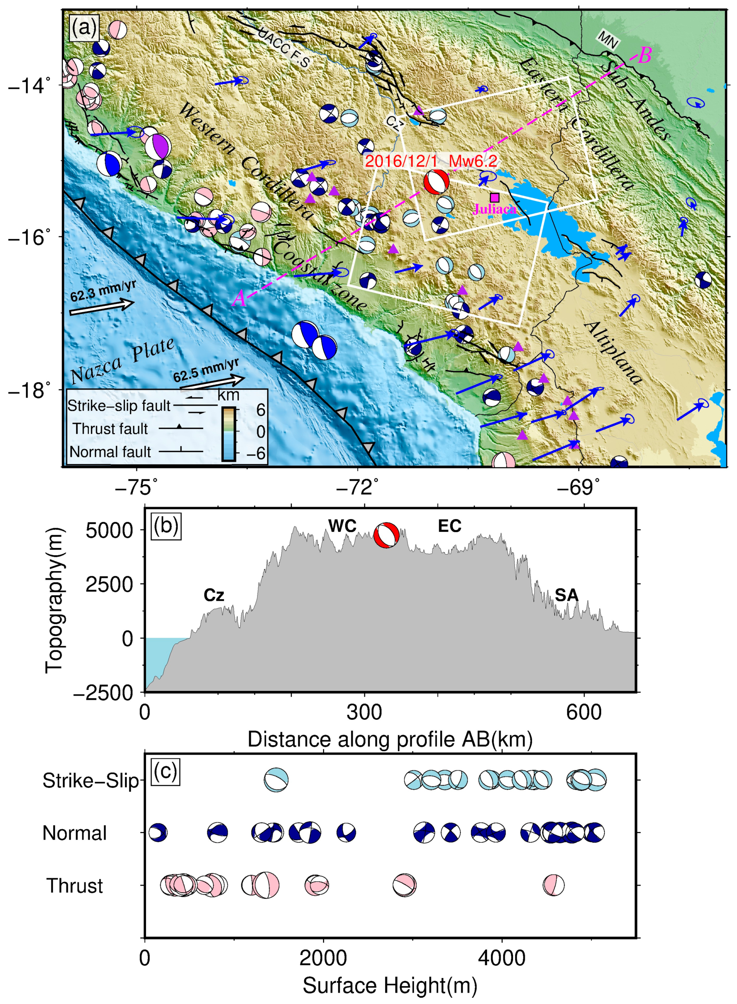
As an active part of the central Andes, the section from 13°S to 19°S experiences different convergence rates from north to south along the Peru Trench (Figure 1a; [4,12]). These variations can lead to complex changes in the geologic processes along the subduction zone, which have great effects on crustal deformation as well as seismic activity all across the central Andes of southern Peru. Numerous earthquakes have occurred in the central Andes of southern Peru in the past, especially along the subduction zone, including some great thrust earthquakes (Mw > 7.5), such as the historical 1942 Mw 8.1 earthquake, the 1996 Mw 7.7 earthquake, the 2001 Mw 8.4 earthquake, and the 2001 Mw 7.6 earthquake (Figure 1a). The frequent occurrence of these great earthquakes indicates a complex tectonic process. In general, the geological structure of the southern Peruvian Andes consists of a forearc region, a volcanic arc, and a back-arc region. However, in detail, the main geological structures are the trench axis, the coastal zone (Cz), the WC, the Altiplano plateau, the EC, and the sub-Andean fold and thrust belt (SA) from west to east (Figure 1a; [13]). All these morphotectonic provinces are different in their style of deformation and topography. Active thrust faults are found in the SA, whereas strike-slip faults and normal faults are mainly concentrated in the Andean highlands (Figure 1a). Moreover, a combination of strike-slip, normal, and thrust faults is seen in the Cz, revealing a complex pattern of deformation (Figure 1a). The maximum elevations in the Cz and SA are both less than 3000 m, whereas the Altiplano plateau has an average elevation of ~3800 m ([14]; Figure 1a). Besides, the peak elevations of the WC and EC exceed 6000 m ([14]; Figure 1a). The 2016 Juliaca earthquake occurred in the highlands of the central Andes at an elevation of approximately 4800 m, and an active volcanic chain is located to the west of the epicenter (Figure 1a). High heat flow that can affect the tectonic evolution and physical properties of the lithosphere is found below the volcanic chain, forearc, and back-arc regions between 15°S and 19°S. But, compared with the high heat flow below the volcanic chain and back-arc, heat flow is relatively low below the forearc [15]. In the east of the epicenter, two fault systems, named the Vilcanota Fault and the Cuzco Fault System, exist and are characterized by normal mechanisms and NW-SE trending (Figure 1a). A large sinistral strike-slip fault known as the Urcos-Ayayiri-Copacabana-Coniri Fault appears to the north of the epicenter and trends NW-SE (Figure 1a). Its slip rate is estimated to be ~2 to 3 mm/yr over the last 2 Ma [16], which indicates relatively low tectonic movement. Seismic data (Figure 1c) show that the majority of crustal thrust earthquakes are limited to elevations less than 3000 m, while normal earthquakes preferentially occur in high regions above 3000 m. The clear relationship between the focal mechanisms and topography indicates that gravitational potential energy (GPE) within the central Andean mountains plays a significant role in controlling the type of crustal deformation [17]. Besides, the authors of the reference [18] investigated the Peruvian Andes and proposed that these shallow and normal-faulting earthquakes near the Andean peaks reflect local shallow extension controlled by gravitational processes.
3. Coseismic Observations
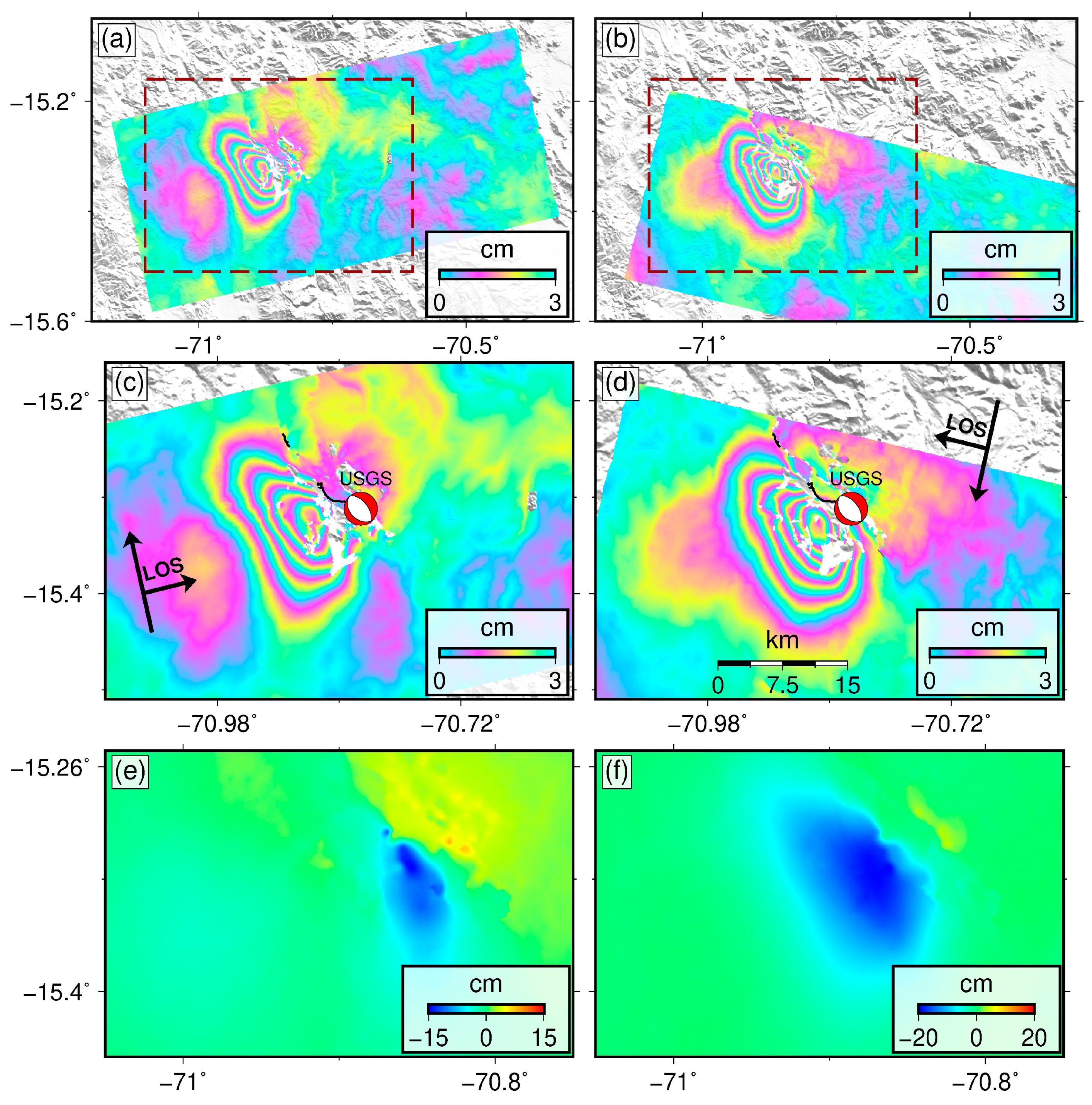
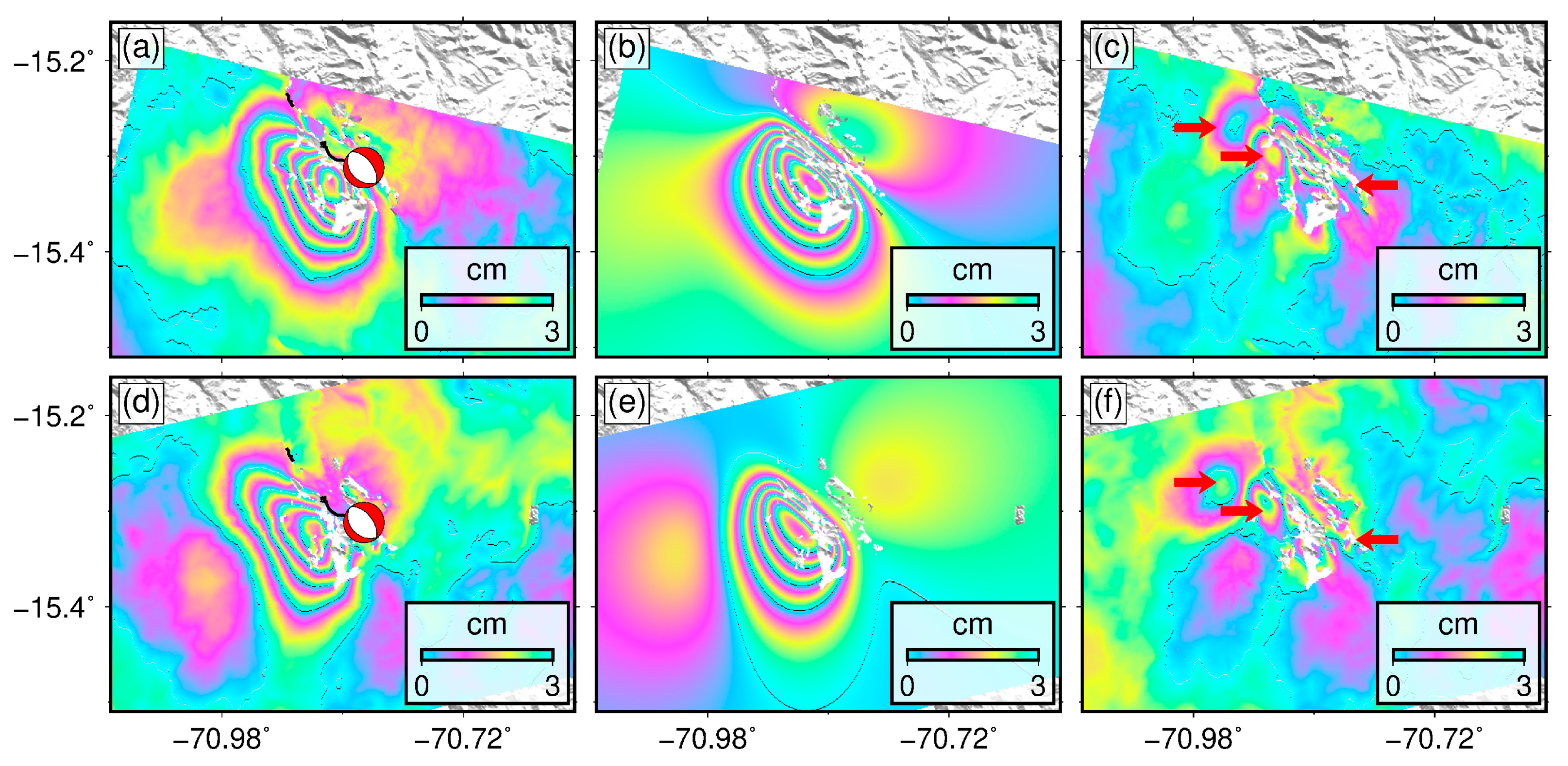
The Sentinel-1A satellite, which collects C-band SAR data using terrain observation with progressive scans (TOPS) mode, is widely used to measure the surface deformation related to earthquakes [19]. In this study, we acquire both the ascending track T149A and the descending track T127D Sentinel-1A SAR data covering the coseismic rupture of the 2016 Juliaca earthquake between 15 November 2016 and 20 December 2016 (Table 2). We use subswath 1 (bursts 3–4) and subswath 2 (bursts 1–2) from tracks T149A and T127D, respectively, to generate the coseismic interferograms of this earthquake. Based on the GAMMA 2022 software [20], we use the two-pass differential SAR interferometry method to process four pairs of single-look complex SAR images with the purpose of obtaining the coseismic deformation of this earthquake. In order to suppress noise to a degree, the multilook ratio between the azimuth and range directions is set at 2:10. An accuracy better than 0.001 pixel in the azimuth direction is required to eliminate possible phase jumps between subsequent bursts [21,22]. After achieving high-quality coregistration results between the TOPS SLC data, the topography phase is removed from the interferogram by using agency-provided precise orbits together with a 30 m digital elevation model [23]. A power spectrum filter [24] is utilized in order to reduce the influence of phase noise, and the branch cut method [25] is used to unwrap the interferograms. Finally, the interferograms are geocoded to the WGS84 geographic coordinates. Moreover, we used a linear function among elevation, location, and error phase, estimated with observations away from the main deformation, to eliminate the topography-correlated atmospheric delays and residual orbital errors [26]. Benefiting from the sparse vegetation in the highlands of the central Andes, clear coseismic surface deformation related to the 2016 Juliaca earthquake is acquired. We can see much denser fringes on the western edge of the major ellipitical deformation region than on the eastern edge of the major ellipitical deformation region in both the ascending and descending interferograms. Besides, the surface rupture trace is also found on the eastern edge of the major ellipitical deformation region. These pieces of evidence support a west-dipping seismogenic fault responsible for the 2016 earthquake. The LOS displacements of the ascending and descending interferograms are up to ~14 cm and ~19 cm, respectively. The ascending and descending interferograms exhibit similar deformation magnitudes and comparable fringe patterns consistent with the major motion away from the satellite, revealing that the surface deformation is characterized by subsidence. A small decorrelation region still exists, which may be a result of the high surface deforamtion gradient and intense damage. Moreover, we acquired the quasi-east-west and quasi-vertical deformations by utilizing the ascending and descending SAR data (a detailed method can be seen in the reference [19]). The result (Figure 2e,f) reveals that the 2016 Juliaca earthquake mainly led to subsidence displacement with a peaking value of ∼20 cm, revealing a normal-faulting mechanism.
4. Postseismic Observations
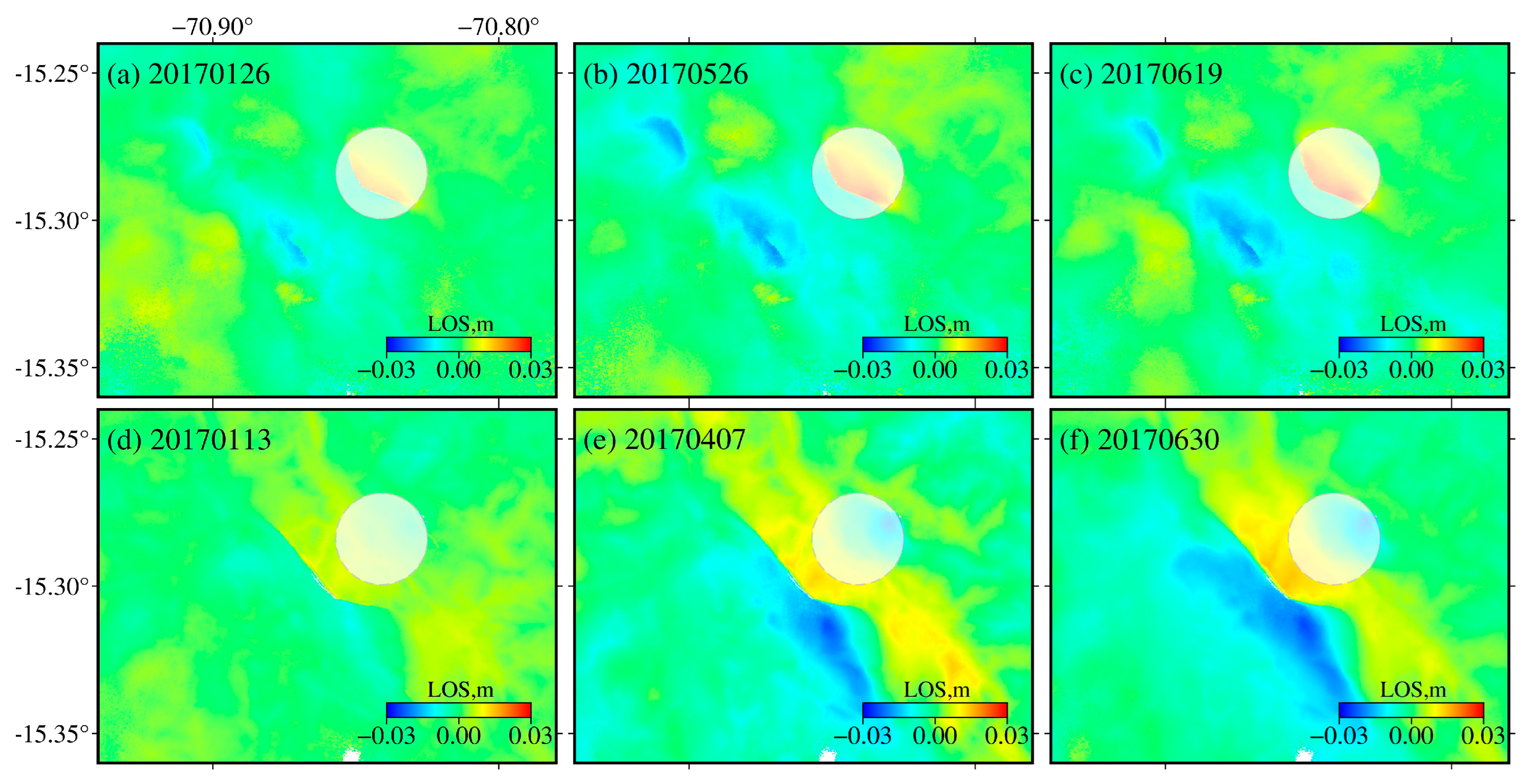
To obtain the postseismic deformation related to the 1 December 2016 Juliaca earthquake, seven Sentinel-1A ascending images spanning the time period from 9 December 2016 to 19 June 2017 and twelve descending images spanning the time period from 20 December 2016 to 30 June 2017 are used (Table 3). We first use the same method to process all the postseismic interferometric pairs as the coseismic interferogram and then apply the MintPy package to acquire the following InSAR time series by means of the small baseline method [27,28,29]. The processing results (Figure 3) exhibit one significant deformation area located at the up-dip region of the greatest coseismic deformation gradient. The cumulative postseismic LOS displacements in the ascending and descending interferograms are up to ~−1.8 cm and ~2.5 cm, respectively, for the 2016 Juliaca event.
5. Results
5.1. Coseismic Inversion
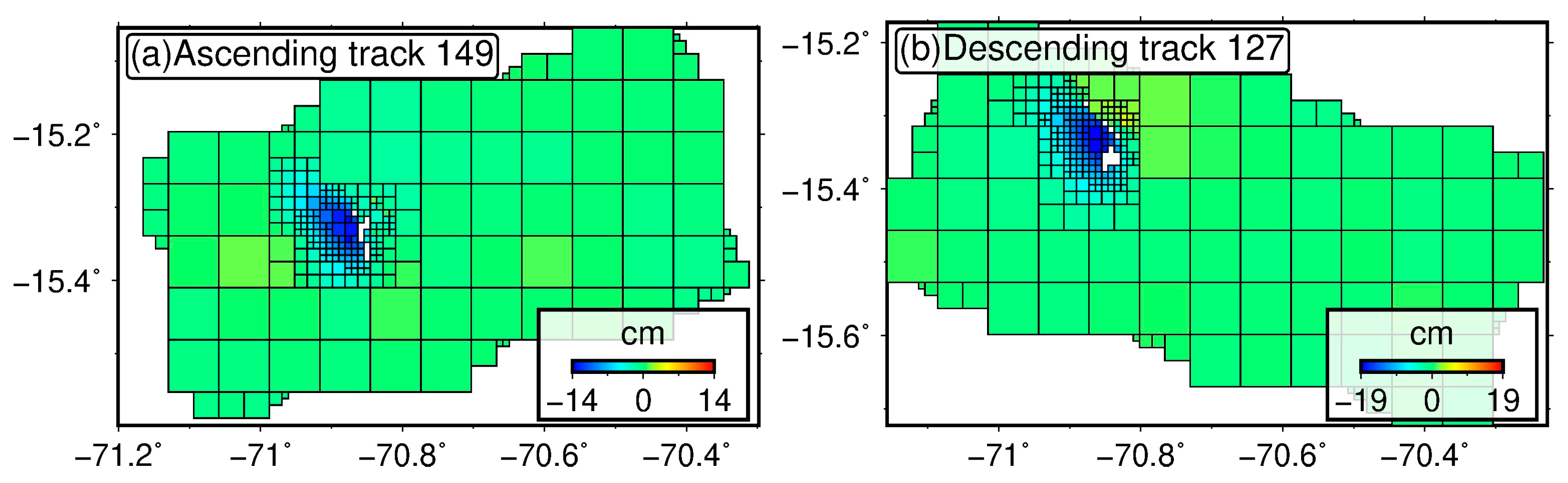
To improve the inversion efficiency, we use the quadtree method to downsample the coseismic deformation of the 2016 Juliaca earthquake (Figure 4). In addition, we apply the empirical errors of these two interferograms obtained from the 1D covariance function to set the weight ratio of the ascending and descending SAR data to be 1:0.987 [30]. On the basis of the rectangular dislocation model [31], the fault geometrical parameters and the detailed coseismic slip distribution of this earthquake were obtained by InSAR observations. An open inversion package called PSOKINV [32] is used to invert for the fault parameters of the one-segment model with a two-step method. First, a nonlinear inversion algorithm is applied to obtain the fault geometric parameters by minimizing the square misfit under the hypothesis of uniform slip on a rectangular fault; then, a linear inversion algorithm is applied to acquire the detailed slip distribution on the determined fault plane.
5.1.1. Uniform Slip Inversion
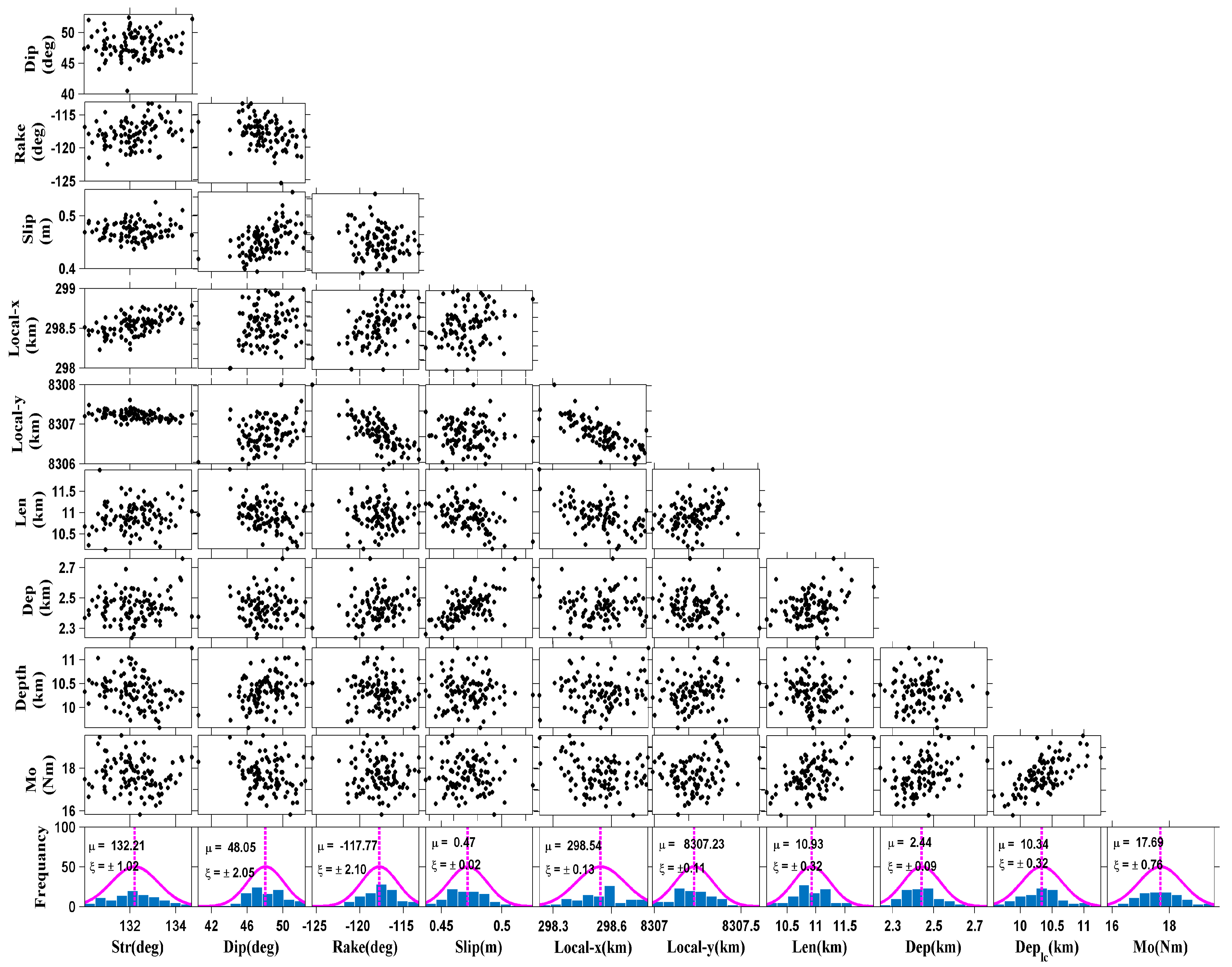
The fault geometry parameters, consisting of fault length, fault width, buried depth, dip, strike, rake, and location, are acquired by minimizing the squared misfits between the observed and modeled coseismic surface deformation [32]. According to the coseismic interferograms of the 2016 earthquake (Figure 1), field investigation [3], and focal mechanism solutions provided by both USGS and GCMT (Table 1), the strike of the rupture fault is constrained between 114° and 154° during the inversions. The uncertainty of fault geometrical parameters is evaluated by means of the Monte Carlo method [33]. Model solutions from 100 simulations disturbed by noise in statistical properties based on the one-dimensional covariance functions are applied to obtain the standard deviation from their distributions (Figure 5). The optimal fault parameters and standard deviations of all final solutions from inversion are shown in Table 1. Our uniform slip model shows that the rupture fault has a dip of ~48° and a strike of ~132°, with a width of ~10.7 km and a length of ~10.9 km. The uniform slip reaches up to 0.47 m and the rake is determined to be ~−118°. The inverted geodetic moment magnitude is Mw 6.13, which is slightly smaller than the GCMT result and the USGS result. As a whole, our optimal fault geometrical parameters are basically consistent with the two previously published studies [1,3] and are relatively stable (Figure 5). Figure 6 shows the modeling results for the uniform slip model. The acquired uniform slip model fits the observed interferograms well except in the epicenter area, where relatively large residual fringes still exist (Figure 6c,f). The root-mean-square error (RMS) between the observed and modeled values is 5.2 mm and 4.5 mm for the ascending track and the descending track, respectively.
5.1.2. Slip Distribution Inversion
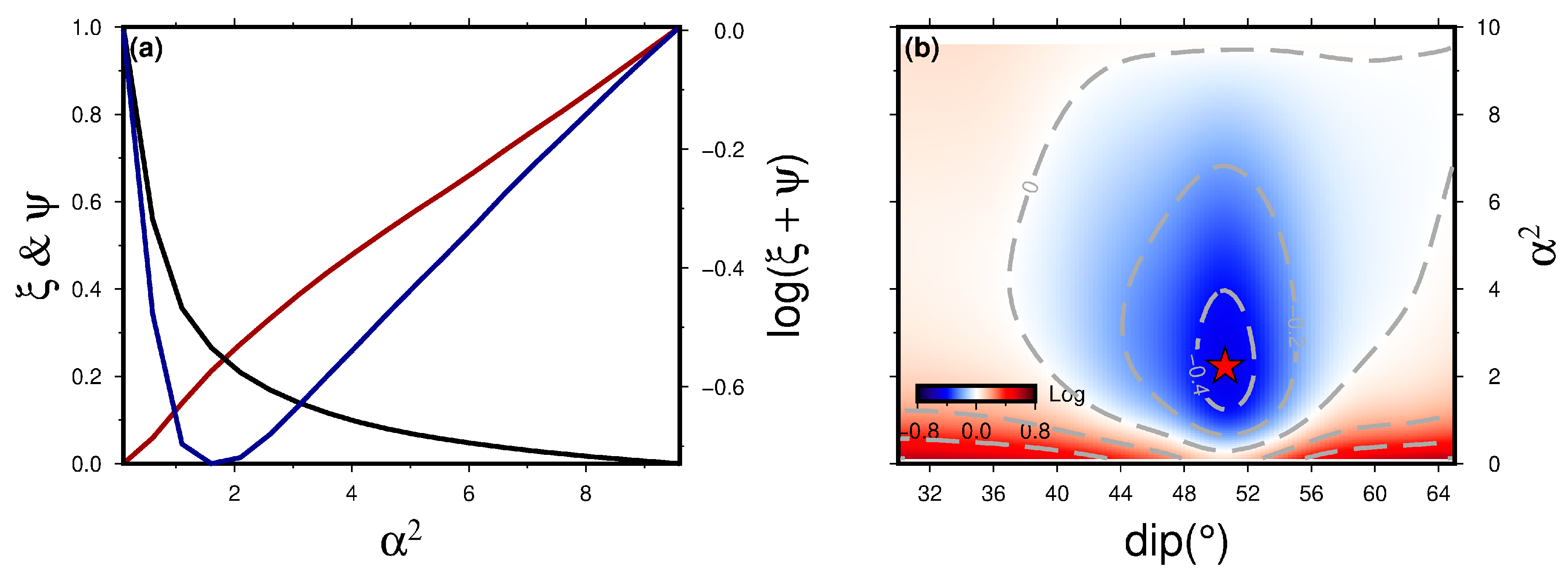
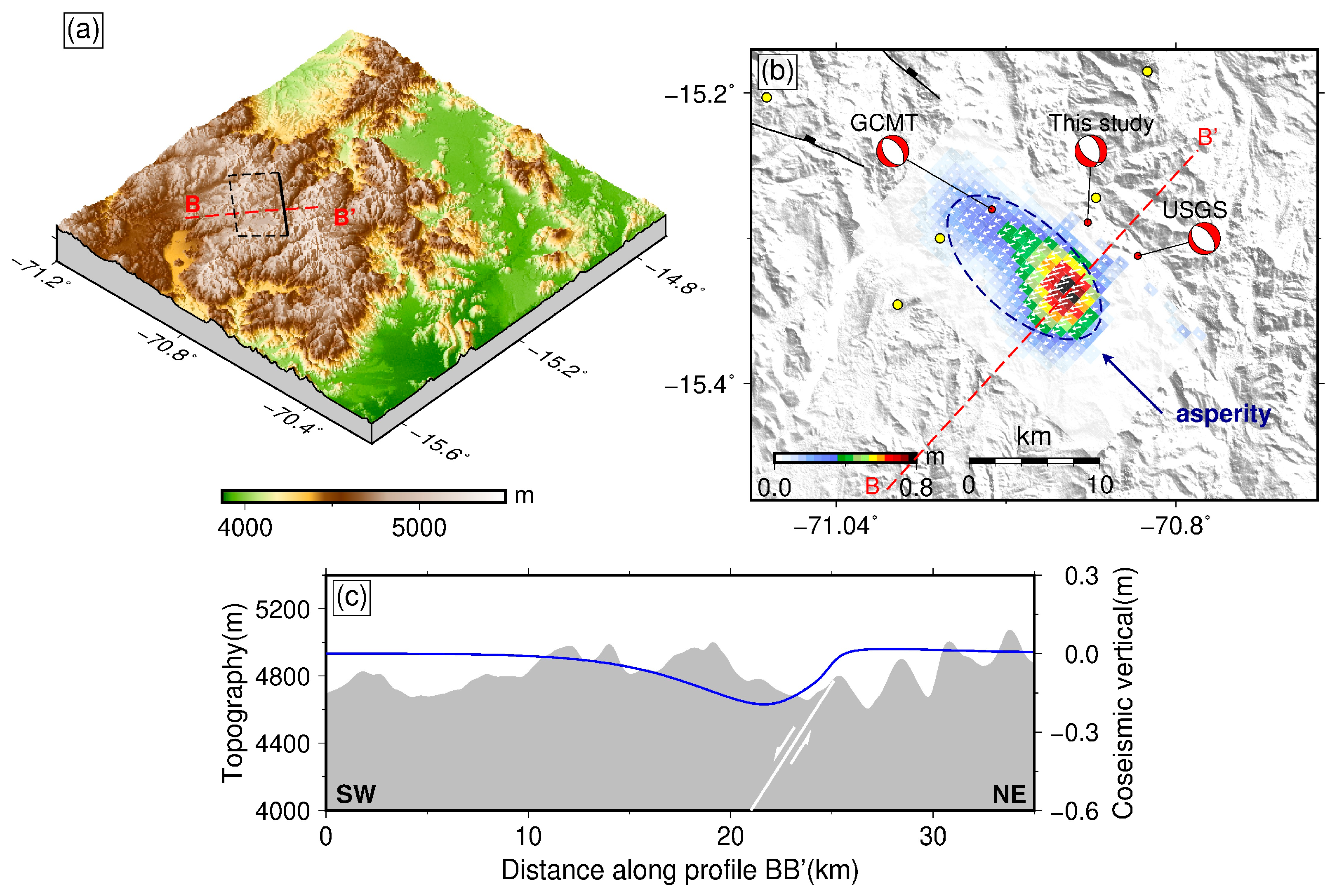
To fully understand the mechanism of regional tectonics, the detailed coseismic slip distribution of the 2016 Juliaca earthquake is inverted from the InSAR observations. Once the fault geometrical parameters are acquired from the uniform slip model, the slips on the rupture fault plane along the dip and strike directions show linear relationships with surface deformation according to the classic linear-elastic dislocation theory [31]. Fixing the fault geometrical parameters for the seismogenic fault plane, we extend the fault width and length to 20 km along the downdip direction and 25 km along the strike direction, respectively. Then, we discretize the fault plane into 500 patches with a size of 1 km by 1 km. In addition, the dip determined from the uniform slip inversion is not always optimal for the slip distribution model [32]. Therefore, we use the grid search method to determine the best-fit dip and the smoothing factor at the same time (e.g., [32]). Therein, a log function is applied as follows: ƒ(δ, α2) = log(Ψ + ξ), where α2, δ, Ψ and ξ are the smoothing factors, dip, slip roughness, and residual. The determined dip and smoothing factor acquired from the log function are 50.6° and 2.2, respectively (Figure 7). Figure 8 shows the best-fit slip distribution model of the 2016 earthquake, indicating that the rupture fault is mainly dominated by normal faulting with some dextral strike-slip components. The maximum values of strike-slip and dip-slip are 0.36 m and 0.7 m, respectively. The fault slip is mainly confined to the depth range of 3–12 km, with a peak slip of ~0.78 m at a depth of 5.4 km (Figure 8b). Furthermore, several slip patches with values of ~0.1 m appear at the surface, suggesting that the coseismic rupture of the 2016 earthquake may have fractured the ground surface, consistent with the field investigation results [3]. The Juliaca earthquake contributes to the NE-SW extensional strain and the thinning of the crust to some extent because of the downward movement of the rupture fault plane (Figure 8b). The coseismic slip distribution releases the geodetic seismic moment of 2.0 × 10¹⁸ N m, equal to Mw 6.14. The moment magnitude of this event is smaller than those provided by the GCMT and USGS, which is attributed to the difference in using observational data. Compared to the modeled results for the uniform slip model (Figure 6), the modeled results for the distributed slip model show an obvious improvement around the surface trace of the rupture fault (Figure 9). The general deformation patterns of the ascending and descending tracks are better matched by the coseismic slip distribution. Only some relatively large errors occur near the fault trace (Figure 9c,f), which may be related to the early postseismic deformation and the signal loss caused by the earthquake in the surrounding area. The RMS between the InSAR observations and the modeled value by our distributed slip model is 4.5 mm and 4.2 mm for the ascending and descending tracks, respectively. The map of topography and coseismic vertical displacement (Figure 8c) shows that the 2016 event clearly occurred on the eastern side of a graben with a steep footwall and that the resulting subsidence is located mainly beneath the relatively low topography. The modeled rupture fault is located to the east of both the high vertical deformation gradient and the high topographic gradient. The high consistency between surface displacement in this earthquake and the local geomorphology indicates that this event may be related to topography and that the SW-NE extensional direction of the rupture fault is controlled by the local topography near the epicenter (e.g., [34]).
5.2. Postseismic Inversion
Poroelastic rebound, afterslip, and viscoelastic relaxation are believed to be the three main mechanisms responsible for postseismic deformation (e.g., [35]). Given the short-period, localized postseismic deformation and shallow depth of the 1 Decenber 2016 Juliaca earthquake, we assume that the identified postseismic deformation is dominated by afterslip. To acquire the detailed afterslip distribution, we perform an inversion with cumulative deformation (Figure 3). Herein, we assume that the afterslip occurred on the same seismogenic fault plane as the coseismic rupture. The result (Figure 10) reveals that the afterslip is mainly characterized by normal faulting and that most of the slip is confined at depths between 0 and 5.4 km, peaking at ~0.05 m at a depth of ~3.8 km. The relatively shallow postseismic afterslip makes up for the coseismic slip deficit area to some extent (Figure 8b and Figure 10). The acquired afterslip distribution can fit the postseismic observation well (Figure 11). The cumulative moment due to afterslip is ~7.5 × 10¹⁶ Nm, corresponding to an Mw 5.2 earthquake.
6. Discussion
6.1. Possible Driving Mechanisms of the 2016 Juliaca Earthquake
Understandably, the occurrence of gravitational collapse often results from changes in the balance of forces that support the thickened crust during lithospheric deformation [36]. When the spreading forces induced by the lateral variations in crustal thickness are large enough or the forces that resist this anomaly decrease, such as the strength of both the deformed and surrounding lithosphere, GPE stored in the thickened crust and high topography during the mountain-building phase can be released through the lateral transfer of crustal material toward lowlands (e.g., [37,38,39]), thus causing collapse and crustal extension in the highlands as well as the occurrence of normal faulting earthquakes in this region.
For the central Andes, the authors of the reference [40] demonstrated that topographic contrast is highly consistent with crustal thickness contrast. Here, we can regard topography as a proxy for crustal thickness. Therefore, the crust and lithosphere below the regions of higher topography reflect intense crustal thickening and a relatively large PGE. Figure 1b shows that elevation decreases from ~5000 m in the WC to ~0 m in the Cz over a lateral distance of only ~110 km and from ~4200 m in the EC to ~1000 m in the SA over a lateral distance of only ~130 km. The sharp topographic gradients between highlands and lowlands, creating the large lateral contrasts in GPE, are believed to induce the large gravitational spreading force that can drive crustal material from the highlands (WC and EC) to the lowlands (Cz and SA) (e.g., [41,42]). For this phenomenon to occur immediately, the resisting force from the strength of the crust also plays a key role (e.g., [43]). However, the presence of high heat flows below both the volcanic chain and the highlands [15] weakens the strength of the crust and makes it less resistant to the gravitational spreading force to some extent [44]. As a result, the large GPE stored in the topography and crustal thickness may relax. The large GPE drives the crustal materials from the WC to the Cz and from the EC to the SA, which could lead to mass loss in the highlands (WC and EC) and accumulation of crustal material in the lowlands (Cz and SA). The highlands begin to experience gravitational collapse to achieve mass balance through isostatic adjustment, while the Cz and the SA experience tectonic compression to accommodate the flow of crustal material from the regions of high GPE. Such a long-term process is thought to produce large internal deformations within the highlands and thus result in the accumulation of substantial strain energy that is eventually released by normal-faulting earthquakes, e.g., [42]. The active normal faults and recent normal earthquakes, mainly concentrated in the highlands of the central Andes (Figure 1a), show some evidence for the present collapse. Moreover, the results of geological investigation show that from the mid-Neogene to the present, tectonic compression is mainly located in the SA rather than in the Cz [45,46], which further supports the geodynamic interpretation that gravitational collapse appears to occur in the high Andes. On the one hand, this GPE-driven crustal material transfer toward the lowlands is facilitated better by the high heat flow below the EC and SA than by the relatively low heat flow below the WC and Cz [15]. On the other hand, in the context of the eastward movement of crustal material over the entire central Andes [10,37], the direction of material flow driven by GPE in the EC is the same as the direction of the eastward movement of crustal material, resulting in the reinforcement of crustal material flow into the SA, whereas the direction of material flow driven by GPE in the WC is opposite to the direction of the eastward movement of crustal material, leading to the offset of the crustal material flow in the Cz. GPE-driven crustal material flow best explains the geological investigations. Meanwhile, the phenomenon that GPE drives the crustal material from the highlands to the lowlands also confirms the occurrence of gravitational collapse in the highlands.
The 2016 Juliaca earthquake, characterized by an extensional fault mechanism (Figure 8b, Table 1), is a typical event in the highlands of southern Peru, which may be experiencing a gravitational collapse. The geodynamic interpretation above is supported by our preferred coseismic and postseismic slip distribution of the 2016 earthquake (Figure 8b and Figure 10). The up-dip normal slip well reflects the gravitational collapse of the lithosphere that is caused by the down-dip mass loss due to the migration of crustal material toward the lowlands (Figure 8b).
6.2. Relationship with Great Historical Earthquakes
The occurrence of great historical earthquakes near the subduction zone of the central Andes can further influence the generation of earthquakes and stress states in the upper plate (e.g., [47]). To investigate whether the effect of the stress caused by historical earthquakes promoted the 2016 Juliaca earthquake, we calculated the coseismic and postseismic Coulomb stress changes (CCS and PCS) caused by the great earthquakes with Mw > 7.5 since 1942, including the 1942 Mw 8.1 earthquake, the 1996 Mw 7.7 earthquake, the 2001 Mw 8.4 earthquake, and the 2001 Mw 7.6 earthquake (Figure 1a), to obtain the stress accumulation state near the epicenter area of the 2016 earthquake. Here, we define the 1942 Mw 8.1 earthquake, the 1996 Mw 7.7 earthquake, the 2001 Mw 8.4 earthquake, and the 2001 Mw 7.6 earthquake as events A, B, C, and D, respectively. During the stress calculation, we use the psgrn/pscmp program, which is based on the viscoelastic-gravitational dislocation theory [48]. The USGS website provides the distributed slip models of events B, C, and D. For event A, we set the strike/dip/rake values of 345°/25°/95° for the rupture fault [7]. The length, width, and maximum displacement of the rupture fault calculated by the Wells and Coppersmith empirical formula [49] are 175 km, 51.4 km, and 6.15 m, respectively. The focal mechanism of the 2016 earthquake (Table 1) is used as the receiver fault. An apparent friction coefficient of 0.4 was applied [50]. Based on Crust1.0, a layered Earth model of the subduction zone was obtained (Table 4). Moreover, the postseismic Coulomb stress due to viscous relaxation is calculated with a viscosity value of 4 × 10¹⁹ for the continental mantle [51]. Finally, we calculate the Coulomb stress changes at a depth of 12 km (the maximum depth at which the fault ruptures). Compared with all the calculated results (Figure 12), event C plays a dominant role in the process of stress evolution. The coseismic stress changes and postseismic stress changes due to event C at the epicenter of the 2016 earthquake are 0.65 bar and 0.03 bar, respectively (Table 5). The total of the Coulomb stress changes of the four events reaches 0.95 bar at the epicenter of the 2016 earthquake (Table 5, Figure 12i), exceeding the commonly accepted triggering threshold of 0.1 bar, which suggests that the four events promoted the generation of the 2016 earthquake.
6.3. Potential Hazards in the Surrounding Area
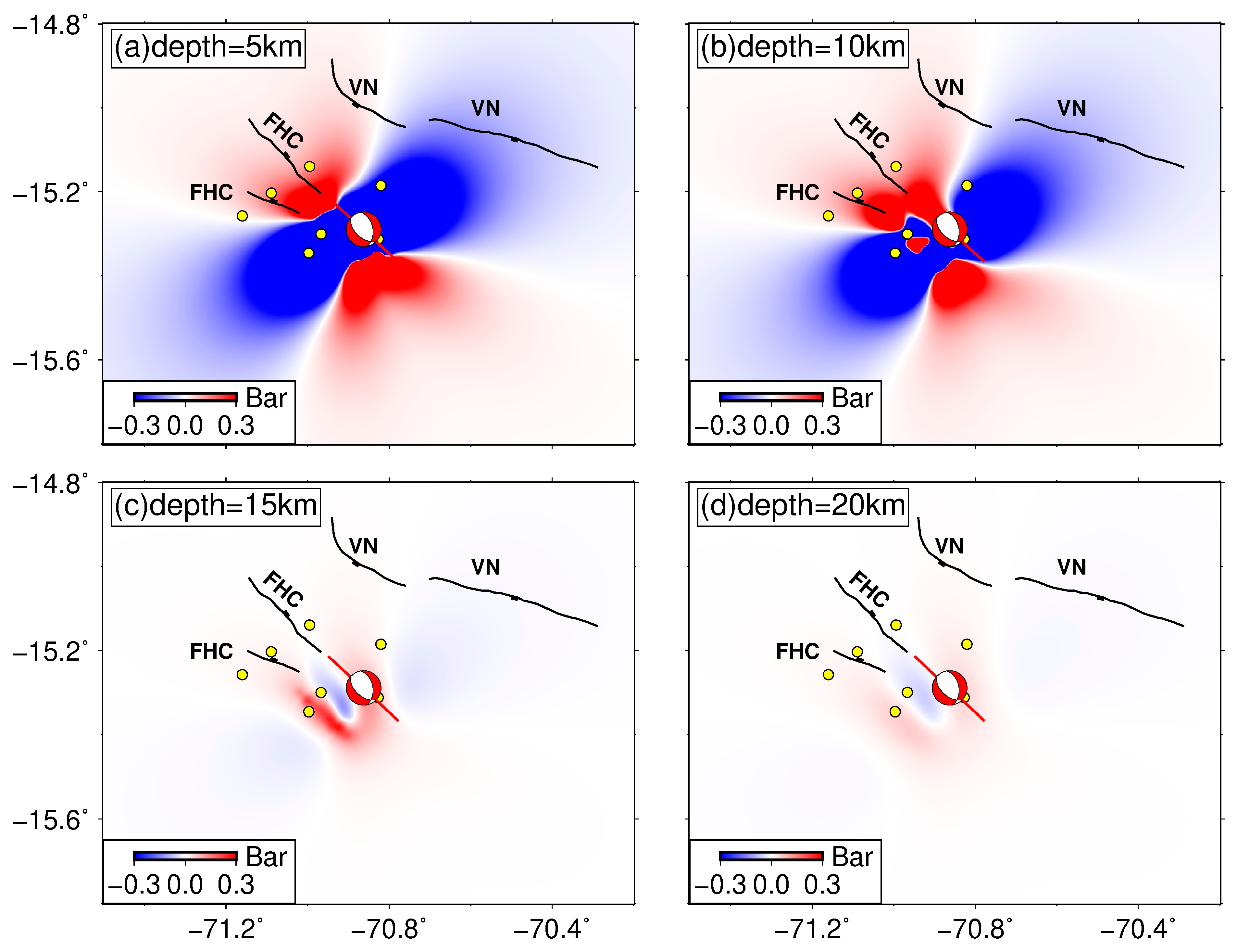
As the largest normal earthquake in the high Andes of southern Peru, the coseismic slip of the 2016 Juliaca earthquake may have a significant effect on the stress state of the adjacent faults and seismicity through stress transfer (e.g., [52,53,54,55,56]). To assess the influence of this event on the nearby mapped fault, we quantified the coseismic Coulomb stress changes. Similar to the method in Section 6.2, the layered Earth model near the epicenter is obtained from Crust1.0 (Table 4). In this study, the distributed slip model inverted is used (Figure 8b). Considering the strike and mechanism of the regionally known faults are similar to the seismogenic fault of the 2016 event, we set the focal mechanism (Table 1) of this event as the receiver mechanism for the mapped faults and applied a typical friction coefficient of 0.4 [50]. The depths of 5 km (at which the maximum slip is located), 10 km, 15 km, and 20 km are chosen as the calculated depths. The results (Figure 13) show that the stress decreases with increasing depth and that the shallow parts of both the Falla Huaytacucho-Condoroma fault (FHC) and the western segment of the Vilcanota Fault System (VN) are in a region with positive Coulomb stress changes greater than 0.1 bar (Figure 13), which indicates relatively high seismic risk. In addition, the eastern segment of VN is located in a region with negative Coulomb stress changes (Figure 13), indicating relatively low seismic risk. Because of the lack of aftershocks, the triggering mechanism of aftershocks is still a challenge for us to investigate. Further research is needed.
7. Conclusions
We apply the coseismic InSAR observation supplemented with the field investigation to explore the fault geometry parameters and detailed coseismic and postseismic slip distribution of the 2016 Juliaca earthquake. In addition, an in-depth analysis of the seismogenic mechanism, the relationship between this event and nearby historical earthquakes, and the detailed stress changes associated with the surrounding mapped active faults is performed. The main conclusions are as follows:
- (1)
- The coseismic rupture of the 2016 Juliaca earthquake is mainly dominated by normal faulting but has some dextral strike-slip components; the coseismic slip is mainly concentrated in the depth range of 2–12 km with a maximum slip of ~0.78 m at a depth of 5.4 km.
- (2)
- The postseismic afterslip with a peaking slip of 0.05 m at a depth of 3.8 km is located at the up-dip part (a depth range of 0–5.4 km) of the rupture fault, partially compensating the coseismic slip deficit.
- (3)
- The 2016 earthquake may be a result of gravitational collapse, and the nearby great historical earthquakes may have promoted the occurrence of this event in advance.
- (4)
- The FHC fault and the western segment of the VN fault should be paid more attention to due to their relatively high stress loading.
Author Contributions
Conceptualization, J.Y. and Q.H.; methodology, Q.H.; software, J.Y.; validation, Q.H., W.J. and J.Y.; formal analysis, W.J.; investigation, W.J.; resources, J.Y.; data curation, Q.H.; writing—original draft preparation, Q.H., W.J. and J.Y.; writing—review and editing, J.Y.; W.J., Q.H. and Y.Z.; visualization, Q.H.; supervision, J.Y.; project administration, J.Y.; funding acquisition, Q.H. All authors have read and agreed to the published version of the manuscript.
Funding
This research was funded by the National Natural Science Foundation of China (Nos. 42277478, 52274169, and 41301598), and Joint Funds of the National Natural Science Foundation of China (No. U21A20109).
Data Availability Statement
The original Sentinel-1 images are downloaded from the European Space Agency (https://scihub.copernicus.eu/dhus/#/home, accessed on 13 July 2023).
Conflicts of Interest
The authors declare no conflict of interest.
References
- Xu, G.; Xu, C.; Wen, Y.; Yin, Z. Coseismic and postseismic deformation of the 2016 Mw 6.2 lampa earthquake, southern peru, constrained by interferometric synthetic aperture radar. J. Geophys. Res. Solid Earth 2019, 124, 4250–4272. [Google Scholar] [CrossRef]
- Aguirre, E.; Benavente, C.; Audin, L.; Wimpenny, S.; Baize, S.; Rosell, L.; Palomino, A. Earthquake surface ruptures on the altiplano and geomorphological evidence of normal faulting in the december 2016 (Mw 6.1) parina earthquake, peru. J. S. Am. Earth Sci. 2021, 106, 103098. [Google Scholar] [CrossRef]
- Wimpenny, S.; Copley, A.; Benavente, C.; Aguirre, E. Extension and Dynamics of the Andes inferred from the 2016 Parina (Huarichancara) Earthquake. J. Geophys. Res. Solid Earth 2018, 123, 8198–8228. [Google Scholar] [CrossRef]
- Kendrick, E.; Bevis, M.; Smalley, R., Jr.; Brooks, B.; Vargas, R.B.; Laurıa, E.; Fortes, L.P.S. The Nazca–South America Euler vector and its rate of change. J. S. Am. Earth Sci. 2003, 16, 125–131. [Google Scholar] [CrossRef]
- Kendrick, E.; Bevis, M.; Smalley, R., Jr.; Brooks, B. An integrated crustal velocity field for the central Andes. Geochem. Geophys. Geosyst. 2001, 2, 11. [Google Scholar] [CrossRef]
- Bevis, M.; Kendrick, E.; Smalley, R.; Brooks, B.; Allmendinger, R.; Isacks, B. On the strength of interplate coupling and the rate of back arc convergence in the central Andes: An analysis of the interseismic velocity field. Geochem. Geophys. Geosyst. 2001, 2, 11. [Google Scholar] [CrossRef]
- Sennson, J.L.; Beck, S.L. Historical 1942 Ecuador and 1942 Peru subduction earthquakes and earthquake cycles along Colombia-Ecuador and Peru subduction segments. Pure Appl. Geophys. 1996, 146, 67–101. [Google Scholar] [CrossRef]
- Coutand, I.; Cobbold, P.R.; Urreiztieta, M.; Gautier, P.; Chauvin, A.; Gapais, D.; López-Gamundí, O. Style and history of Andean deformation, Puna plateau, northwestern Argentina. Tectonics 2001, 20, 210–234. [Google Scholar] [CrossRef]
- Echavarria, L.; Hernández, R.; Allmendinger, R.; Reynolds, J. Subandean thrust and fold belt of northwestern Argentina: Geometry and timing of the Andean evolution. AAPG Bull. 2003, 87, 965–985. [Google Scholar] [CrossRef]
- Gregory-Wodzicki, K.M. Uplift history of the Central and Northern Andes: A review. Geol. Soc. Am. Bull. 2000, 112, 1091–1105. [Google Scholar] [CrossRef]
- Beck, S.L.; Zandt, G. The nature of orogenic crust in the central Andes. J. Geophys. Res. Solid Earth 2002, 107, ESE-7. [Google Scholar] [CrossRef]
- Somoza, R. Updated azca (Farallon)-South America relative motions during the last 40 My: Implications for mountain building in the central Andean region. J. S. Am. Earth Sci. 1998, 11, 211–215. [Google Scholar] [CrossRef]
- Giovanni, M.K.; Horton, B.K.; Garzione, C.N.; McNulty, B.; Grove, M. Extensional basin evolution in the Cordillera Blanca, Peru: Stratigraphic and isotopic records of detachment faulting and orogenic collapse in the Andean hinterland. Tectonics 2010, 29, 6. [Google Scholar] [CrossRef]
- Garzione, C.N.; Hoke, G.D.; Libarkin, J.C.; Withers, S.; MacFadden, B.; Eiler, J.; Ghosh, P.; Mulch, A. Rise of the Andes. Science 2008, 320, 1304–1307. [Google Scholar] [CrossRef] [PubMed]
- Springer, M.; Förster, A. Heat-flow density across the Central Andean subduction zone. Tectonophysics 1998, 291, 123–139. [Google Scholar] [CrossRef]
- Sébrier, M.; Mercier, J.L.; Mégard, F.; Laubacher, G.; Carey-Gailhardis, E. Quaternary normal and reverse faulting and the state of stress in the central Andes of south Peru. Tectonics 1985, 4, 739–780. [Google Scholar] [CrossRef]
- Molnar, P.; Tapponnier, P. Active tectonics of Tibet. J. Geophys. Res. Solid Earth 1978, 83, 5361–5375. [Google Scholar] [CrossRef]
- Villegas-Lanza, J.C.; Chlieh, M.; Cavalié, O.; Tavera, H.; Baby, P.; Chire-Chira, J.; Nocquet, J.M. Active tectonics of Peru: Heterogeneous interseismic coupling along the Nazca megathrust, rigid motion of the Peruvian Sliver, and Subandean shortening accommodation. J. Geophys. Res. Solid Earth 2016, 121, 7371–7394. [Google Scholar] [CrossRef]
- Wen, Y.; Xu, C.; Liu, Y.; Jiang, G. Deformation and source parameters of the 2015 Mw 6.5 earthquake in Pishan, western China, from Sentinel-1A and ALOS-2 data. Remote Sens. 2016, 8, 134. [Google Scholar] [CrossRef]
- Werner, C.; Wegmüller, U.; Strozzi, T.; Wiesmann, A. Gamma SAR and interferometric processing software. In Proceedings of the ERS-ENVISAT Symposium, Gothenburg, Sweden, 16–20 October 2000; Volume 1620, p. 1620. [Google Scholar]
- Yagüe-Martínez, N.; Prats-Iraola, P.; Gonzalez, F.R.; Brcic, R.; Shau, R.; Geudtner, D.; Bamler, R. Interferometric processing of Sentinel-1 TOPS data. IEEE Trans. Geosci. Remote Sens. 2016, 54, 2220–2234. [Google Scholar] [CrossRef]
- Wegnüller, U.; Werner, C.; Strozzi, T.; Wiesmann, A.; Frey, O.; Santoro, M. Sentinel-1 support in the GAMMA software. Procedia Comput. Sci. 2016, 100, 1305–1312. [Google Scholar] [CrossRef]
- Farr, T.G.; Rosen, P.A.; Caro, E.; Crippen, R.; Duren, R.; Hensley, S.; Seal, D. The shuttle radar topography mission. Rev. Geophys. 2007, 45, 2. [Google Scholar] [CrossRef]
- Goldstein, R.M.; Werner, C.L. Radar interferogram filtering for geophysical applications. Geophys. Res. Lett. 1998, 25, 4035–4038. [Google Scholar] [CrossRef]
- Goldstein, R.M.; Zebker, H.A.; Werner, C.L. Satellite radar interferometry: Two-dimensional phase unwrapping. Radio Sci. 1998, 23, 713–720. [Google Scholar] [CrossRef]
- Cavalié, O.; Doin, M.P.; Lasserre, C.; Briole, P. Ground motion measurement in the Lake Mead area, Nevada, by differential synthetic aperture radar interferometry time series analysis: Probing the lithosphere rheological structure. J. Geophys. Res. Solid Earth 2007, 112, B03403. [Google Scholar] [CrossRef]
- Zhang, Y.; Fattahi, H.; Amelung, F. Small baseline InSAR time series analysis: Unwrapping error correction and noise reduction. Comput. Geosci. 2019, 133, 104331. [Google Scholar]
- Fattahi, H.; Amelung, F. DEM error correction in InSAR time series. IEEE Trans. Geosci. Remote Sens. 2013, 51, 4249–4259. [Google Scholar] [CrossRef]
- Fattahi, H.; Amelung, F. InSAR observations of strain accumulation and fault creep along the Chaman Fault system, Pakistan and Afghanistan. Geophys. Res. Lett. 2016, 43, 8399–8406. [Google Scholar] [CrossRef]
- Hanssen, R.F. Radar Interferometry: Data Interpretation and Error Analysis; Kluwer Academic: Dordrecht, The Netherlands; Boston, MA, USA, 2001; Volume 2. [Google Scholar]
- Okada, Y. Surface deformation due to shear and tensile faults in a half-space. Bull. Seismol. Soc. Am. 1985, 75, 1135–1154. [Google Scholar] [CrossRef]
- Feng, W.; Li, Z.; Elliott, J.R.; Fukushima, Y.; Hoey, T.; Singleton, A.; Xu, Z. The 2011 Mw 6.8 Burma earthquake: Fault constraints provided by multiple SAR techniques. Geophys. J. Int. 2013, 195, 650–660. [Google Scholar] [CrossRef]
- Parsons, B.; Wright, T.; Rowe, P.; Andrews, J.; Jackson, J.; Walker, R.; Khatib, M.; Tablebian, M.; Bergman, E.; Engdahl, E.R. The 1994 Sefidabeh (eastern Iran) earthquakes revisited: New evidence from satellite radar interferometry and carbonate dating about the growth of an active fold above a blind thrust fault. Geophys. J. Int. 2006, 164, 202–217. [Google Scholar] [CrossRef]
- Elliott, J.R.; Walters, R.J.; England, P.C.; Jackson, J.A.; Li, Z.; Parsons, B. Extension on the Tibetan plateau: Recent normal faulting measured by InSAR and body wave seismology. Geophys. J. Int. 2010, 183, 503–535. [Google Scholar] [CrossRef]
- Wang, K.; Fialko, Y. Space geodetic observations and models of postseismic deformation due to the 2005 M7. 6 Kashmir (Pakistan) earthquake. J. Geophys. Res. Solid Earth 2014, 119, 7306–7318. [Google Scholar] [CrossRef]
- England, P.C.; Houseman, G.A. The mechanics of the Tibetan Plateau. Philosophical Transactions of the Royal Society of London. Ser. A Math. Phys. Sci. 1988, 326, 301–320. [Google Scholar]
- Liu, M. Cenozoic extension and magmatism in the North American Cordillera: The role of gravitational collapse. Tectonophysics 2001, 342, 407–433. [Google Scholar] [CrossRef]
- Artyushkov, E.V. Stresses in the lithosphere caused by crustal thickness inhomogeneities. J. Geophys. Res. 1973, 78, 7675–7708. [Google Scholar] [CrossRef]
- McKenzie, D. Active tectonics of the Mediterranean region. Geophys. J. Int. 1972, 30, 109–185. [Google Scholar] [CrossRef]
- Beck, S.L.; Zandt, G.; Myers, S.C.; Wallace, T.C.; Silver, P.G.; Drake, L. Crustal-thickness variations in the central Andes. Geology 1996, 24, 407–410. [Google Scholar] [CrossRef]
- Dewey, J.F. Extensional collapse of orogens. Tectonics 1988, 7, 1123–1139. [Google Scholar] [CrossRef]
- Wang, S.; Xu, C.; Xu, W.; Yin, Z.; Wen, Y.; Jiang, G. The 2017 Mw 6.6 Poso Earthquake: Implications for Extrusion Tectonics in Central Sulawesi. Seismol. Res. Lett. 2018, 90, 649–658. [Google Scholar] [CrossRef]
- Rey, P.; Vanderhaeghe, O.; Teyssier, C. Gravitational collapse of the continental crust: Definition, regimes and modes. Tectonophysics 2001, 342, 435–449. [Google Scholar] [CrossRef]
- Viti, M.; Mantovani, E.; Albarello, D. On The Plausibility of The Gravitational Collapse As Driving Mechanism For Tectonic Extension. In Proceedings of the EGS General Assembly Conference Abstracts, Nice, France, 21–26 April 2002; Volume 27. [Google Scholar]
- Isacks, B.L. Uplift of the central Andean plateau and bending of the Bolivian orocline. J. Geophys. Res. Solid Earth 1998, 93, 3211–3231. [Google Scholar] [CrossRef]
- Sheffels, B.M. Lower bound on the amount of crustal shortening, in the central Bolivian Andes. Geology 1990, 18, 812–815. [Google Scholar] [CrossRef]
- Hayes, G.P.; Smoczyk, G.M.; Benz, H.M.; Furlong, K.P.; Villaseñor, A. Seismicity of The Earth 1900–2013, Seismotectonics of South America (Nazca Plate Region) (No. 2015-1031-E); US Geological Survey: Reston, VA, USA, 2015. [Google Scholar]
- Wang, R.; Lorenzo-Martín, F.; Roth, F. PSGRN/PSCMP-a new code for calculating co-and post-seismic deformation, geoid and gravity changes based on the viscoelastic-gravitational dislocation theory. Comput. Geosci. 2006, 32, 527–541. [Google Scholar] [CrossRef]
- Wells, D.L.; Coppersmith, K.J. New empirical relationships among magnitude, rupture length, rupture width, rupture area, and surface displacement. Bull. Seismol. Soc. Am. 1994, 84, 974–1002. [Google Scholar]
- Freed, A.M. Earthquake triggering by static, dynamic, and postseismic stress transfer. Annu. Rev. Earth Planet. Sci. 2005, 33, 335–367. [Google Scholar] [CrossRef]
- Li, S.; Moreno, M.; Bedford, J.; Rosenau, M.; Oncken, O. Revisiting viscoelastic effects on interseismic deformation and locking degree: A case study of the Peru-North Chile subduction zone. J. Geophys. Res. Solid Earth 2015, 120, 4522–4538. [Google Scholar] [CrossRef]
- Stein, R.S.; Barka, A.A.; Dieterich, J.H. Progressive failure on the North Anatolian fault since 1939 by earthquake stress triggering. Geophys. J. Int. 1997, 128, 594–604. [Google Scholar] [CrossRef]
- Toda, S.; Stein, R.S.; Reasenberg, P.A.; Dieterich, J.H.; Yoshida, A. Stress transferred by the 1995 Mw = 6.9 Kobe, Japan, shock: Effect on aftershocks and future earthquake probabilities. J. Geophys. Res. Solid Earth 1998, 103, 24543–24565. [Google Scholar] [CrossRef]
- Mildon, Z.K.; Toda, S.; Faure Walker, J.P.; Roberts, G.P. Evaluating models of Coulomb stress transfer: Is variable fault geometry important? Geophys. Res. Lett. 2016, 43, 12407–12414. [Google Scholar] [CrossRef]
- Sboras, S.; Lazos, I.; Bitharis, S.; Pikridas, C.; Galanakis, D.; Fotiou, A.; Chatzipetros, A.; Pavlides, S. Source modelling and stress transfer scenarios of the October 30, 2020 Samos earthquake: Seismotectonic implications. Turk. J. Earth Sci. 2021, 30, 699–717. [Google Scholar] [CrossRef]
- Toda, S.; Enescu, B. Rate/state Coulomb stress transfer model for the CSEP Japan seismicity forecast. Earth Planets Space 2011, 63, 171–185. [Google Scholar] [CrossRef]
Figure 1.
(a) Geological map around the 2016 Mw 6.2 Juliaca earthquake. White arrows represent the convergence rate of the Nazca Plate relative to the South American Plate [4]. Blue arrows show the GPS observations [5]. Purple triangles are active volcanoes [6]. White boxes outline the spatial coverage of the Sentinel-1A SAR images. All the crustal earthquakes (Mw > 5) with depths < 80 km from 1976 to 2016 in the overriding plate are shown. The light blue, dark blue, and pink beach balls represent normal, strike-slip, and thrust faulting earthquakes, respectively. The red beach ball indicates the focal mechanism of the 2016 Juliaca earthquake. The black beach balls from north to south denote the 1942 Mw 8.1 earthquake, the 1996 Mw 7.7 earthquake, 2001 Mw 8.4 earthquake, and 2001 Mw 7.6 earthquake near the subduction zone. Except for the focal mechanism of the 1942 earthquake acquired from the reference [7], all the focal mechanisms are obtained from the GCMT (https://www.globalcmt.org/CMTsearch.html, accessed on 13 July 2023). UACC F. S: Urcos-Ayayiri-Copacabana-Coniri Fault System; VN: Vilcanota Fault; CZ: Cuzco Fault System; MN: Manu thrust fault. (b) Topographic profile along AB marked by the dashed magenta line in (a). Cz: Coastal zone; WC: Western Cordillera; EC: Eastern Cordillera; SA: the sub-Andean fold and thrust belt. (c) Crustal earthquake mechanism versus surface height.

Figure 2.
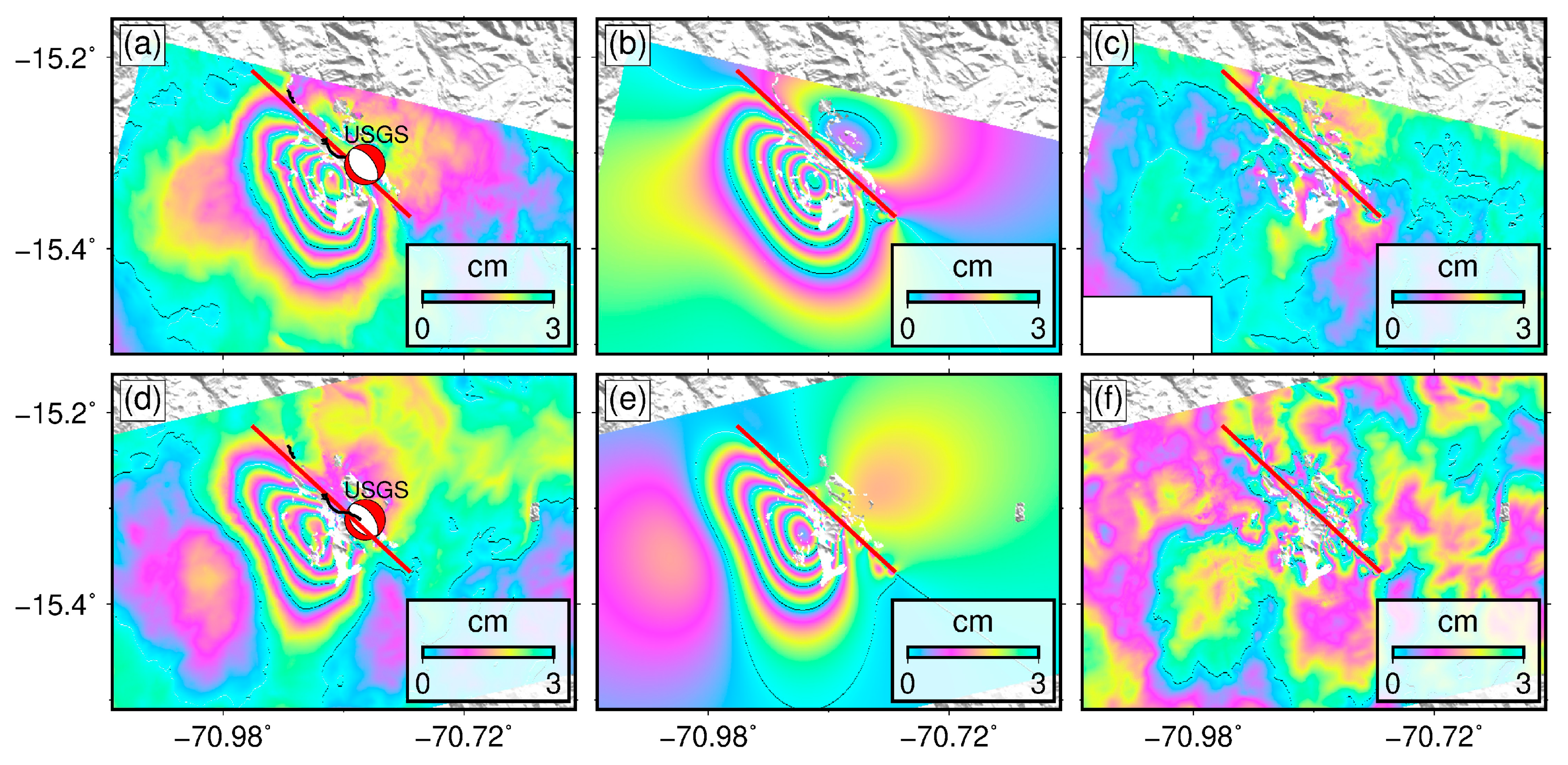
(a,b) are the coseismic interferograms from the ascending track 149 and descending track 127, respectively. The two dark-red dotted boxes represent the areas in (c,d), respectively. The thin black lines in (c,d) represent the surface rupture traces acquired by field investigation [3]. The red beach ball represents the focal mechanism solution of the 2016 Juliaca earthquake. (e,f) are the acquired coseismic quasi-east-west and quasi-vertical deformations, respectively.
Figure 2.
(a,b) are the coseismic interferograms from the ascending track 149 and descending track 127, respectively. The two dark-red dotted boxes represent the areas in (c,d), respectively. The thin black lines in (c,d) represent the surface rupture traces acquired by field investigation [3]. The red beach ball represents the focal mechanism solution of the 2016 Juliaca earthquake. (e,f) are the acquired coseismic quasi-east-west and quasi-vertical deformations, respectively.

Figure 3.
Ascending and descending postseismic time series of the 2016 Juliaca earthquake observed at different time intervals, respectively. White circles show the abnormal deformation, which is not used in the postseismic afterslip inversion.
Figure 3.
Ascending and descending postseismic time series of the 2016 Juliaca earthquake observed at different time intervals, respectively. White circles show the abnormal deformation, which is not used in the postseismic afterslip inversion.

Figure 4.
(a,b) are the ascending and descending down-sampled coseismic interferograms, respectively, which are used to the coseismic inversion.
Figure 4.
(a,b) are the ascending and descending down-sampled coseismic interferograms, respectively, which are used to the coseismic inversion.

Figure 5.
Source parameters of the 2016 Mw 6.2 Juliaca earthquake from the Monte-Carlo analysis. Histograms show distribution in individual model parameter.
Figure 5.
Source parameters of the 2016 Mw 6.2 Juliaca earthquake from the Monte-Carlo analysis. Histograms show distribution in individual model parameter.

Figure 6.
(a,d) are the observed interferograms for the ascending track and descending track, respectively. (b,e) are the modeled interferograms utilizing the acquired uniform slip model. (c,f) are the residual interferograms. Thick red arrows show the areas with relatively large errors.
Figure 6.
(a,d) are the observed interferograms for the ascending track and descending track, respectively. (b,e) are the modeled interferograms utilizing the acquired uniform slip model. (c,f) are the residual interferograms. Thick red arrows show the areas with relatively large errors.

Figure 7.
(a) A trade-off line related to the slip distribution model with a dip of 50.6°. The red and black lines represent the trends of the model roughness and residuals, respectively. The blue line shows log (ξ + ψ). (b) Contour map of log (ξ + ψ) with different dip angles and smoothing factors. Red star represents the global minimum.

Figure 8.
(a) 3D topography map. The thick black line indicates the surface fault trace and the dashed black lines represent the outline of the rupture fault at depth. The dashed red line represents the profile BB’. (b) Coseismic slip distribution model of the 2016 earthquake. Yellow circles are the aftershocks (Mw > 2.5) 15 days after the mainshock from USGS. (c) Topographic profile and coseismic vertical displacement (solid blue line) modeled by the coseismic slip distribution model along BB’. White line with white arrows represents the location of the rupture fault.

Figure 9.
(a,d) are the observed ascending and descending coseismic interferograms, respectively. (b,e) are the modeled interferograms using the distributed slip model. (c,f) are the residual interferograms. The red line is the fault surface trace.
Figure 9.
(a,d) are the observed ascending and descending coseismic interferograms, respectively. (b,e) are the modeled interferograms using the distributed slip model. (c,f) are the residual interferograms. The red line is the fault surface trace.

Figure 10.
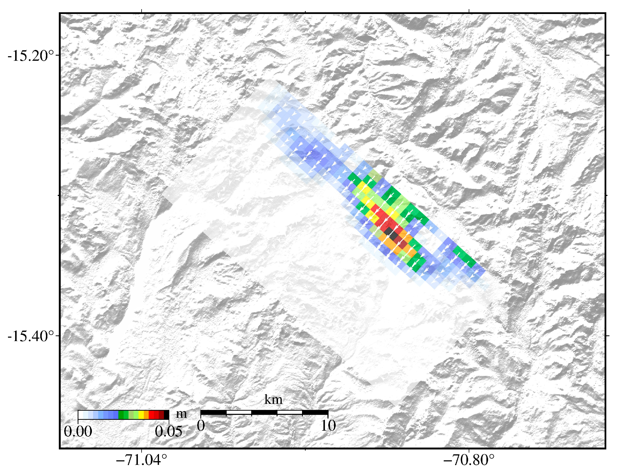
Surface projection of the postseismic afterslip distribtion of the 2016 Juliaca earthquake. The white arrows represent the slip direction.
Figure 10.
Surface projection of the postseismic afterslip distribtion of the 2016 Juliaca earthquake. The white arrows represent the slip direction.

Figure 11.
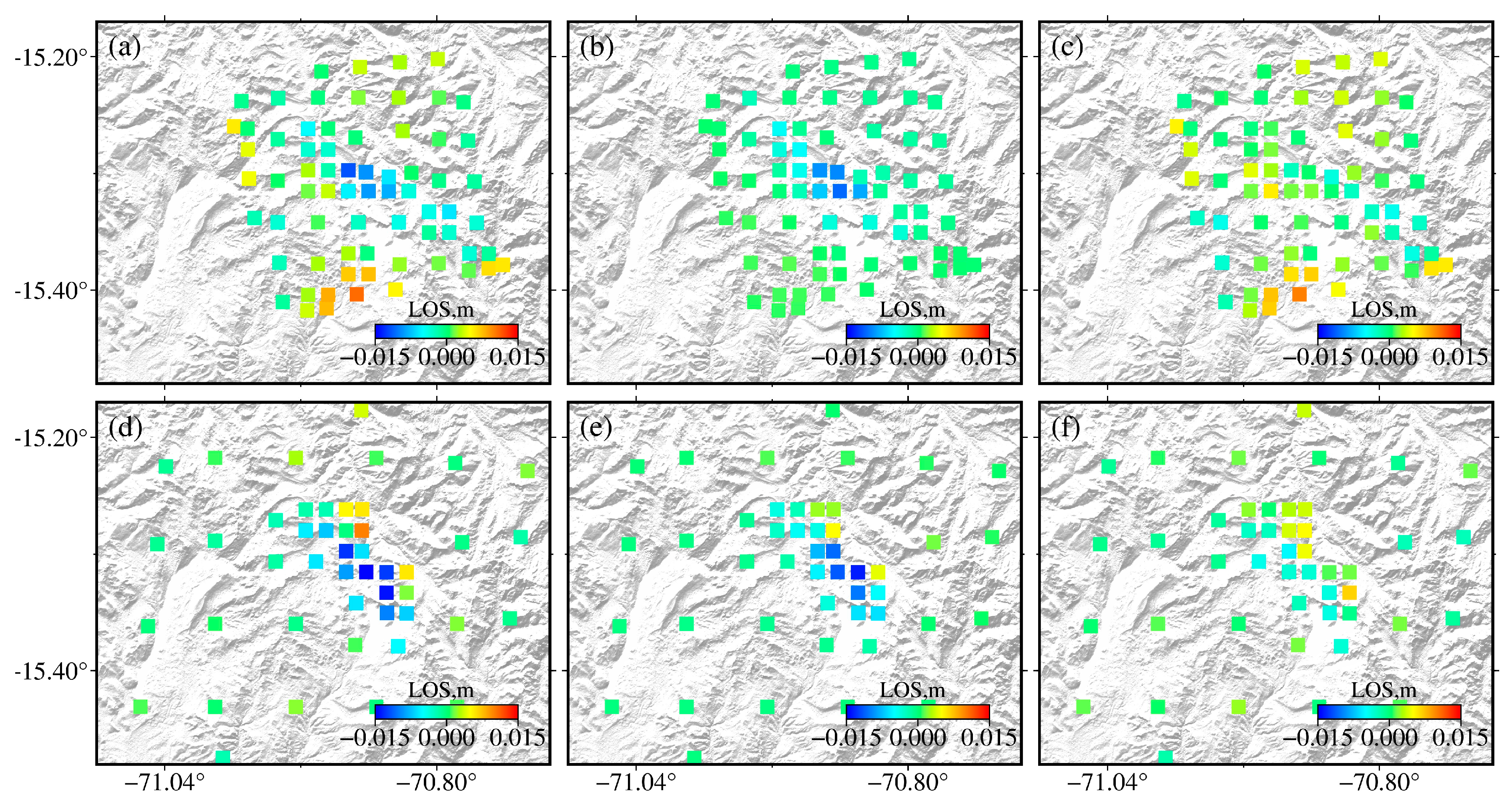
(a,d) are the observed ascending and descending down-sampled data, respectively. (b,e) are the corresponding modeled data. (c,f) are the residuals.
Figure 11.
(a,d) are the observed ascending and descending down-sampled data, respectively. (b,e) are the corresponding modeled data. (c,f) are the residuals.

Figure 12.
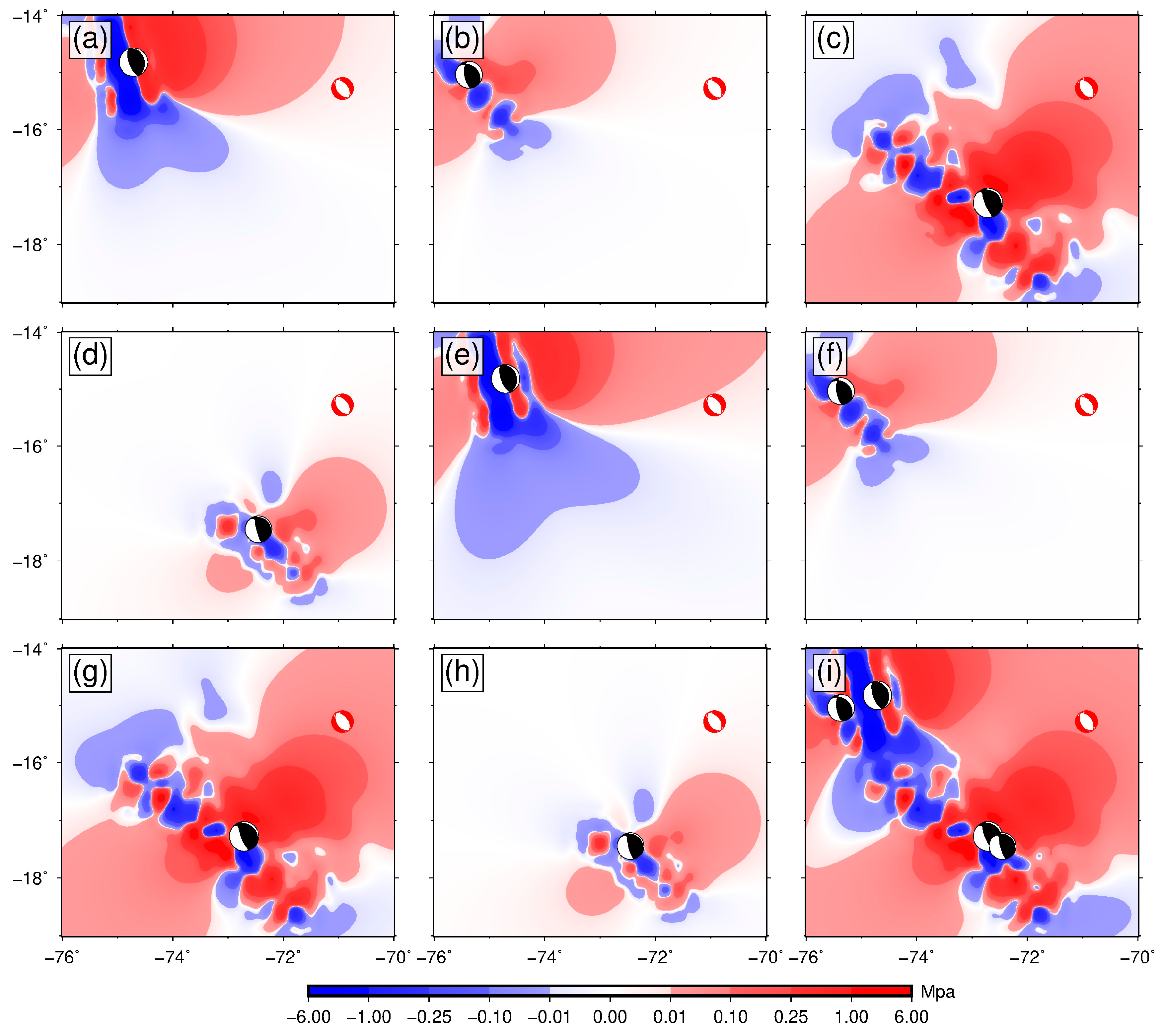
Coulomb stress changes at the epicenter of the 2016 earthquake. (a–d) are coseismic Coulomb stress changes for events A–D, respectively. (e–h) are the sum of the coseismic and postseismic stress changes for events A–D, respectively. (i) is the Coulomb stress accumulation state after the four events. The black beach balls represent the focal mechanism solutions of the events A–D while the red beach ball represents the focal mechanism solutions of the 2016 Juliaca event.
Figure 12.
Coulomb stress changes at the epicenter of the 2016 earthquake. (a–d) are coseismic Coulomb stress changes for events A–D, respectively. (e–h) are the sum of the coseismic and postseismic stress changes for events A–D, respectively. (i) is the Coulomb stress accumulation state after the four events. The black beach balls represent the focal mechanism solutions of the events A–D while the red beach ball represents the focal mechanism solutions of the 2016 Juliaca event.

Figure 13.
Coseismic Coulomb stress changes induced by the 2016 Juliaca earthquake. (a–d) are the Coulomb stress changes at depths of 5 km, 10 km, 15 km and 20 km, respectively. The red line represents the seismogenic fault of the 2016 event. Black lines with a black box are normal faults. FHC: Falla Huaytacucho-Condoroma fault from the SARA database (https://sara.openquake.org/, accessed on 13 July 2023).


Table 1.
Source parameters of the 1 December 2016 Mw 6.2 Juliaca earthquake.
| Model | Lon/° | Lat/° | Strike/° | Dip/° | Rake/° | Length/km | Depth/km | Slip/m | Mw |
|---|---|---|---|---|---|---|---|---|---|
| USGS | −70.827 | −15.312 | 134/324 | 35/56 | −97/−85 | - | 12 | - | 6.2 |
| GCMT | −70.93 | −15.28 | 148/322 | 43/47 | −86/−94 | - | 12.7 | - | 6.2 |
| U-S-model | 6.13 |
Notes: U-S-model are Uniform slip model. Depth shows the center of the upper boundary of the uniform rupture fault plane while the location (Lon and Lat) of the U-S-model is the center of the coseismic rupture surface trace.
Table 2.
Detailed SAR information applied for coseismic deformation of the 1 December 2016 Mw 6.2 Juliaca earthquake.
Table 2.
Detailed SAR information applied for coseismic deformation of the 1 December 2016 Mw 6.2 Juliaca earthquake.
| Satellite | Track | Reference Date | Repeat Date | Perp. B (m) | Inc. Angle | Azi. Angle |
|---|---|---|---|---|---|---|
| Sentinel-1A | T149A | 15 November 2016 | 9 December 2016 | −15 | 33.6 | −12.1 |
| Sentinel-1A | T127D | 26 November 2016 | 20 December 2016 | 112 | 39.0 | −167.8 |
Perp. B: Perpendicular baseline; Azi. Angle: Azimuth angle; Inc. Angle: Incidence angle.
Table 3.
Details of SAR data used for postseismic deformation of the 1 December 2016 Mw 6.2 Juliaca earthquake.
Table 3.
Details of SAR data used for postseismic deformation of the 1 December 2016 Mw 6.2 Juliaca earthquake.
| Satellite | Track | Reference Date | Date Due | No. of Images |
|---|---|---|---|---|
| Sentinel-1A | T149A | 9 December 2016 | 19 June 2017 | 7 |
| Sentinel-1A | T127D | 20 December 2016 | 30 June 2017 | 12 |
Table 4.
Layered crustal model of the Subduction zone.
| Depth/km | VP/km/s | VS/km/s | Density/g/cm3 |
|---|---|---|---|
| 0~7.76 | 6.000 | 3.500 | 2720 |
| 7.76~17.6 | 6.600 | 3.800 | 2860 |
| 17.6~34 | 7.100 | 3.900 | 3050 |
| 34~∞ | 8.040 | 4.470 | 3310 |
Table 5.
Coulomb stress changes caused by the coseismic and postseismic effects of the 1942 Mw 8.1 earthquake, 1996 Mw 7.7 earthquake, 2001 Mw 8.4 earthquake, and 2001 Mw 7.6 earthquake at the epicenter area of 2016 Juliaca earthquake (Unit: Bar).
Table 5.
Coulomb stress changes caused by the coseismic and postseismic effects of the 1942 Mw 8.1 earthquake, 1996 Mw 7.7 earthquake, 2001 Mw 8.4 earthquake, and 2001 Mw 7.6 earthquake at the epicenter area of 2016 Juliaca earthquake (Unit: Bar).
| Coulomb Stress Changes | 1942 Mw 8.1 Earthquake | 1996 Mw 7.7 Earthquake | 2001 Mw 8.4 Earthquake | 2001 Mw 7.6 Earthquake |
|---|---|---|---|---|
| CCS | 0.05472 | 0.008309 | 0.6491 | 0.1742 |
| PCS | 0.01504 | 0.001751 | 0.0287 | 0.0164 |
| CCS + PCS | 0.06976 | 0.01006 | 0.6778 | 0.1906 |
Disclaimer/Publisher’s Note: The statements, opinions and data contained in all publications are solely those of the individual author(s) and contributor(s) and not of MDPI and/or the editor(s). MDPI and/or the editor(s) disclaim responsibility for any injury to people or property resulting from any ideas, methods, instructions or products referred to in the content. |
© 2023 by the authors. Licensee MDPI, Basel, Switzerland. This article is an open access article distributed under the terms and conditions of the Creative Commons Attribution (CC BY) license (https://creativecommons.org/licenses/by/4.0/).
Share and Cite
MDPI and ACS Style
Hu, Q.; Jia, W.; Yang, J.; Zhao, Y. Insight into the 1 December 2016 Mw 6.2 Juliaca Earthquake, Southern Peru, by InSAR Observations and Field Investigation. Remote Sens. 2023, 15, 4341. https://doi.org/10.3390/rs15174341
AMA Style
Hu Q, Jia W, Yang J, Zhao Y. Insight into the 1 December 2016 Mw 6.2 Juliaca Earthquake, Southern Peru, by InSAR Observations and Field Investigation. Remote Sensing. 2023; 15(17):4341. https://doi.org/10.3390/rs15174341
Chicago/Turabian StyleHu, Qingfeng, Weiwei Jia, Jiuyuan Yang, and Yanling Zhao. 2023. "Insight into the 1 December 2016 Mw 6.2 Juliaca Earthquake, Southern Peru, by InSAR Observations and Field Investigation" Remote Sensing 15, no. 17: 4341. https://doi.org/10.3390/rs15174341
Note that from the first issue of 2016, this journal uses article numbers instead of page numbers. See further details here.