Article

Spectral Characteristics of Beached Sargassum in Response to Drying and Decay over Time

by
Chris J. Chandler
1,*,
Silvia Valery Ávila-Mosqueda
2,
Evelyn Raquel Salas-Acosta
2,
Eden Magaña-Gallegos
2,
Edgar Escalante Mancera
2,
Miguel Angel Gómez Reali
2,
Betsabé de la Barreda-Bautista
1,
Doreen S. Boyd
1,
Sarah E. Metcalfe
1,
Sofie Sjogersten
3,
Brigitta van Tussenbroek
2,
Rodolfo Silva
4 and
Giles M. Foody
1
1
School of Geography, University of Nottingham, University Park, Nottingham NG7 2RD, UK
2
Unidad Académica de Sistemas Arrecifales, Instituto de Ciencias del Mar y Limnología, Universidad Nacional Autónoma de México, Puerto Morelos 77580, Mexico
3
School of Biosciences, University of Nottingham, College Road, Sutton Bonington, Loughborough, Leicestershire LE12 5RD, UK
4
Instituto de Ingeniería, Universidad Nacional Autónoma de México, Mexico City 04510, Mexico
*
Author to whom correspondence should be addressed.
Remote Sens. 2023, 15(17), 4336; https://doi.org/10.3390/rs15174336
Submission received: 20 May 2023 / Revised: 7 August 2023 / Accepted: 24 August 2023 / Published: 2 September 2023
(This article belongs to the Section Environmental Remote Sensing)

Abstract

:
The bloom of pelagic Sargassum in the Atlantic Ocean has become increasingly problematic, especially when the algae have beached. A build-up of decaying beached material has damaging effects on coastal ecosystems and tourism industries. While remote sensing offers an effective tool to assess the spatial and temporal patterns of Sargassum over large spatial extents, its use so far has been limited to a broad discrimination of Sargassum species from other macroalgae and floating vegetation. Knowledge on the spatial distribution of decayed material will help to support management strategies and inform targeted removal. In this study, we aim to characterise the spectral response of fresh and decayed Sargassum and identify regions of the spectra that offer the greatest separability for the detection and classification of decayed material. We assessed the spectral response of fresh and decayed Sargassum (1) in situ on the beach and (2) in mesocosm experiments where Sargassum samples were allowed to decay over time. We found a decrease in the magnitude of reflectance, noticeably in the visible region (400–700 nm), for decayed, in contrast to fresh, Sargassum. Separability analyses also showed that most spectral bands with a wavelength > ~540 nm will be capable of discriminating between fresh and decayed material, although the near-infrared region offers the greatest degree of separability. We demonstrate, for the first time, that there are clear differences in the spectral reflectance of fresh and decayed Sargassum with potential application for remote sensing approaches.

1. Introduction

The quantity of seaweed beaching along coastlines around the world has increased substantially in recent years [1]. The build-up of decaying algal biomass can have damaging impacts on coastal ecosystems, livelihoods and tourism industries [2,3,4].
Since 2011, the Caribbean coast has experienced unprecedented influxes of pelagic-drifting Sargassum spp. [5], most commonly Sargassum natans and Sargassum fluitans [6,7]. Chavez et al., 2020 documented monthly averages of 3.2 × 10³ and 1.7 × 10³ m3/km/month for 2018 and 2019, respectively, along the Mexican Caribbean beaches [8]. Decayed masses cast onshore can also be returned to the sea which can convert the often clear coastal waters to a brown colour, often referred to as Sargassum brown-tide [9].
Therefore, understanding the spatial patterns of Sargassum is critical in order to predict its occurrence and help quantify the impact on coastal environments. Remote sensing provides a tool to monitor and assess Sargassum beaching events which otherwise would require ground-based assessments of Sargassum distribution and abundance which can be both time- and labour-intensive.
Previous studies have differentiated Sargassum in the sea from other floating vegetation (e.g., [10]). Field-measurements have found that Sargassum has a distinctive reflectance response at ~630 nm, due to its chlorophyll c pigments [11], and therefore both satellite and airborne instruments have been used to detect and monitor the distribution of Sargassum in the ocean [5,10,11,12,13,14,15,16].
While the remote detection of Sargassum improves our capacity to assess spatial and temporal patterns (see, [17]), knowledge on the degree of decay will further help to inform management strategies and support the targeted removal of such material. Appropriate management of Sargassum is critical for hoteliers, environmental authorities and those responsible for public health, as decomposition on the coast has potentially harmful effects on human health, as it produces toxic gases such as sulphuric acid and ammonia [8,18,19]. On the other hand, if the Sargassum is harvested when fresh, it could be used for a range of purposes with economic and ecological benefits [20,21,22].
Little research has focused on the remote sensing of decaying Sargassum. Recently, a preliminary assessment of the changing spectral response of Sargassum as it decays was undertaken using multi-spectral Sentinel-2 MSI imagery [23]. Until now, no study has assessed detailed, high-spectral-resolution differences in the spectral response of fresh and decayed Sargassum. Doing so will be a fundamental step in order to detect and assess the extent, movement and distribution of decayed Sargassum using satellite-based remote sensing. Widely available remote sensing platforms such as PlanetScope and Sentinel provide a cost-effective tool to repeatedly assess large spatial areas. This, in turn, will help to provide insights into the mechanisms that drive spatial patterns in the distribution and abundance of Sargassum and will reveal patterns that do not emerge at the scale of field-based measurements.
In this study, we aim to characterise the spectral response of Sargassum in different states: fresh, dry, mixed (fresh and dry) and decayed. We also identify regions of the spectra that are most effective at discriminating between fresh and decayed Sargassum. To achieve this, we assessed spectral measurements taken in situ on the beach as well as in mesocosm experiments where Sargassum samples were allowed to decay over time.

2. Materials and Methods
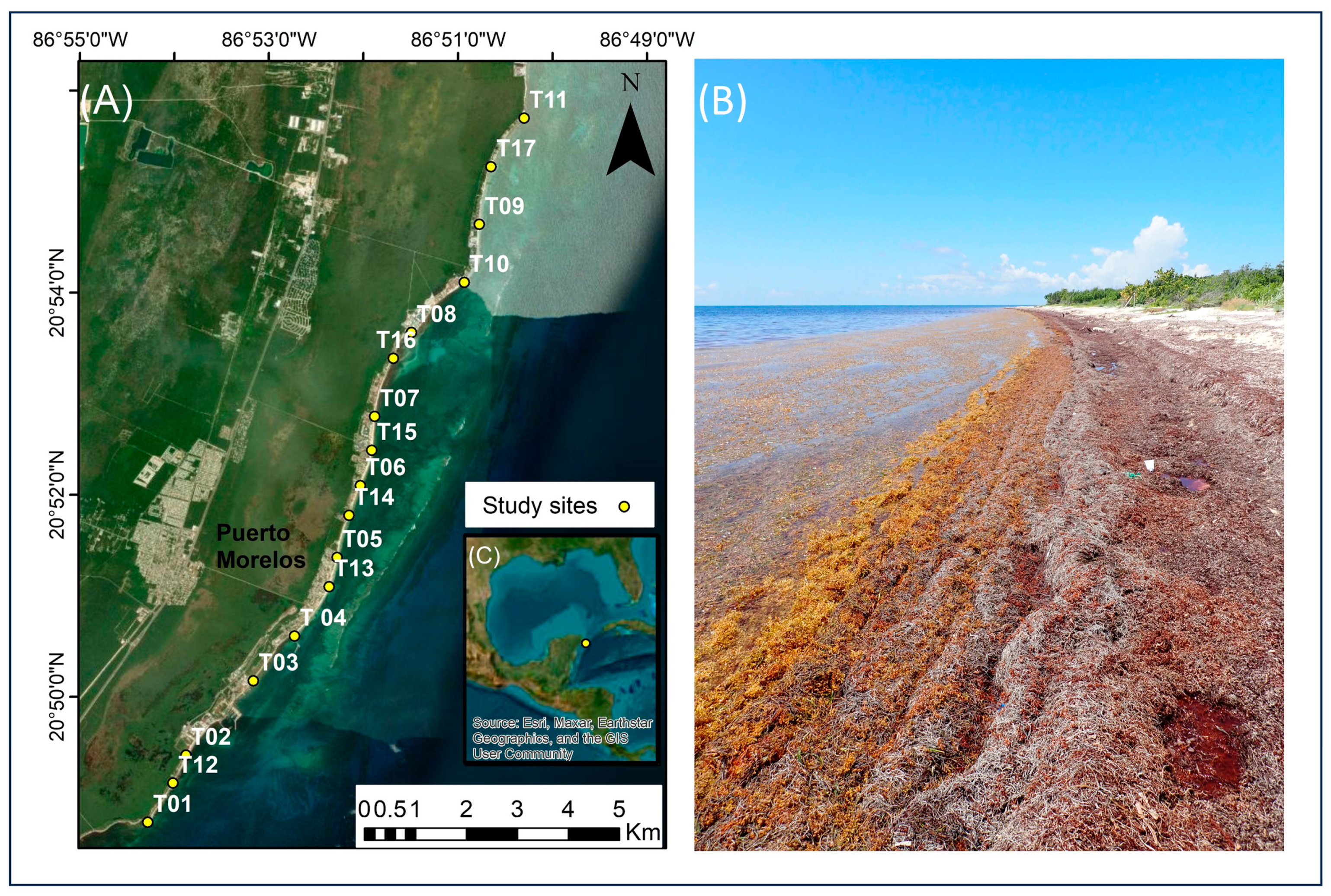
2.1. Study Area

The study area is situated along the Mexican Caribbean coastline near Puerto Morelos, in the state of Quintana Roo (Figure 1). Puerto Morelos (20.8662°N, 86.8686°W) is located 20 km south of the tropical beach resorts of Cancun and has a large, protected area (21 km length and 5 km width) which supports a biodiverse ecosystem and attracts a large number of tourists each year. The beach is NE–SW oriented (20°), composed of carbonate sand of biogenic origin. The region has a microtidal regime with semidiurnal spring and neap tidal ranges of 0.32 and 0.07 m, respectively. The region has a tropical climate with two seasons (summer and winter). In summer, easterly winds are dominant with speeds of 3–9 ms−1. The maximum air temperature is in August with a monthly average of 29 °C [24].
Field data were collected between May and August 2021. A total of 17 locations were chosen at random along the coast of Puerto Morelos (Figure 1). Each location was visited at least twice, and in some cases three times, in order to capture spectral measurements in different states (Table S1). At each sampling location, a transect line was set up perpendicular to the coastline. The sampling area was defined as five metres either side of the transect line.
Since 2011, this coastline, and surrounding areas, have experienced repeated large influxes of Sargassum spp., notably Sargassum fluitans and S. natans, making this a suitable location to assess the spectral characteristics of Sargassum at varying abundances and stages of decomposition. Dense seagrass meadows cover the bottom of the reef lagoon areas [25].

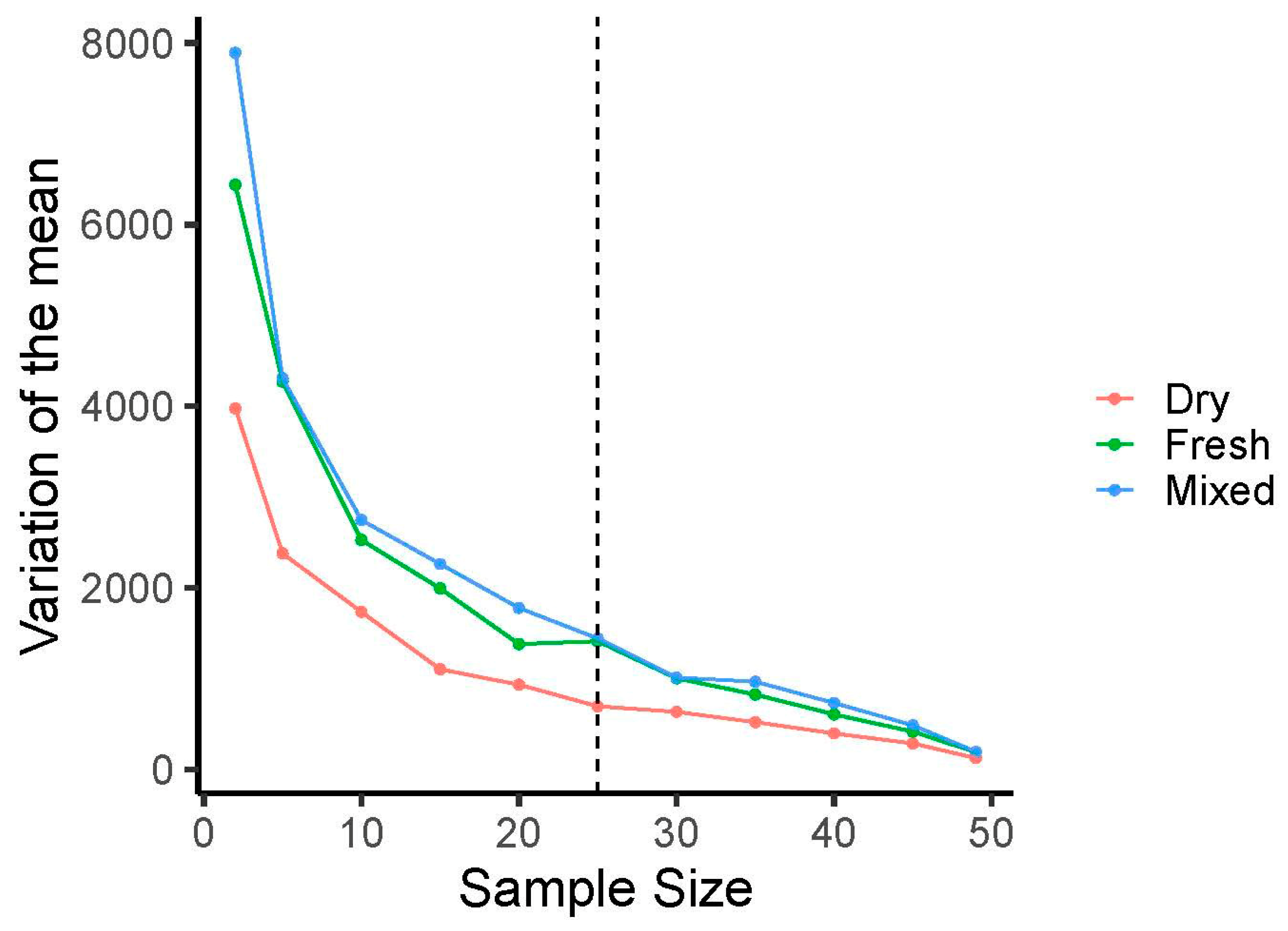
2.2. Spectral Data Collection

Spectral data collected from the beach were obtained using an Analytical Spectral Device (ASD) FieldSpec Pro spectroradiometer (NERC Field Spectroscopy Facility, University of Edinburgh, UK) which acquired high-resolution data from a wide spectral range (350–2500 nm). Spectral data were sampled at intervals of 1.4 nm within the visible-to-near infrared (VNIR) range (350–100 nm), and 2 nm within the shortwave infrared (SWIR) range (1000–2500 nm). The spectral resolution was 3 nm at 700 nm and 10 nm at 1400 nm. The field-of-view was 18 degrees at a distance of approximately 10 cm between the ground surface and the sensor.
Spectral data collected from controlled mesocosm environments were obtained using a GER1500 spectrometer with a spectral range of 350–1050 nm. Data were sampled at 1.5 nm intervals to produce a spectral resolution of 3.2 nm. The field-of-view was 15 degrees and the distance between the surface and the sensor was kept at 10 cm. The use of two different spectrometers was used to avoid unnecessarily moving equipment once the mesocosm experiment was set up. Two different sensors also allowed a comparison of spectra reflectance from two independent sources.
The condition of Sargassum was visually assessed to locate samples within four different states: fresh, dry, mixed (mix of fresh and dry), or decayed (see Supplementary Materials for further information on the different states). A quadrat was randomly placed to define an area to subsample within each class. Within each quadrat, we obtained 25 spectral measurements. Prior testing showed that 25 spectral samples was a sufficient number in order to derive an average spectral signal with no substantial further decrease in the standard deviation of the mean with additional measurements (Figure 2). We randomly selected two spectral measurements and measured the mean value of reflectance for each wavelength and averaged this to calculate an overall mean value. This was repeated 100 times and then the standard deviation of all 100 values was calculated to derive the variation of the mean. This entire process was repeated for increasing samples of spectral measurements, specifically 5, 10, 15, 20, 25, 30, 35, 40, 45, 50. The resulting standard deviation of the means was then plotted to visualise the point at which the variation does not substantially decrease with an increasing sample size (Figure 2).
Optimisation, including dark current readings, was carried out before recording spectral reflectance at each quadrat (approximately every 15 min) to adjust the sensitivity of the instrument’s detectors to illumination conditions at the time of the measurements. A white reference was also obtained, using a calibration plate (Spectralon, Labsphere, Sutton, NH, USA), before recording spectral measurements and after every five measurements to ensure that the quality of white reflectance was maintained for an accurate calculation of reflectance data. All measurements were taken on days with sunny weather conditions, between 11 am and 2 pm (UTC-5), to decrease variation in irradiance which could impact the spectral data collected. However, when frequent optimisation and white reference scans were recorded, we found that changeable weather conditions did not appear to have a large impact on the spectral response (F(1,34) = 1.516, p = 0.227; Figure S1).
Spectral measurements of Sargassum were also obtained outside, in a controlled environment (mesocosms), to determine the differences between the spectral responses of fresh and decayed seaweed. By conducting the experiment in a mesocosm, the impact of external factors such as weather conditions could be reduced in an attempt to highlight changes in spectral characteristics.
Sargassum was collected from the sea and added to 16 mesocosm units (18 L). The experiment consisted of four sets, each containing four individual units. The temperature within each experiment varied, specifically Experiment 1: 22 °C; Experiment 2: 25 °C; Experiment 3: 28 °C; and Experiment 4: 31 °C. Spectral measurements were recorded at the beginning of the experiment and after 10, 15 and 20 days to assess the effect of degradation on the spectral response. We obtained the average spectral measurements across different temperatures and species to capture the variation in spectral responses. Thus, the results show the average spectral responses for each four sets of experiments across four time periods. Three spectral measurements were removed due to equipment errors.

2.3. Identifying Spectra Regions of Greatest Separability

To identify bands that may be most effective at discriminating between classes, we assessed the Jeffries–Matusita (J–M) distance [26]. The J–M distance is a function of separability that directly relates to the probability of how good a resultant classification will be. The J–M distance is asymptotic to 2, whereby values of 2 suggest complete separability between classes. Spectra from fresh samples (n = 4) and decayed samples (n = 4) collected from the mesocosm experiment were used to assess for separability. The separability was assessed for each band (n = 511) and plotted against the wavelength to identify bands of the greatest importance. The degree of separability was also assessed in relation to commonly used remote sensing platforms such as Planet Scope and Sentinel-2 sensors to determine which spectral bands may be most beneficial when using multispectral satellite-derived imagery. The separability metric was calculated using the ‘spatialEco’ package [27] in R [28].
A principal component analysis (PCA) was also conducted to assess the contribution of spectral bands to principal components. A PCA was performed using the prcomp function in R [28]. The standardisation (μ = 0) of variables was performed prior to the PCA. The contribution of the variables was determined using the ‘factoextra’ package [29].

3. Results

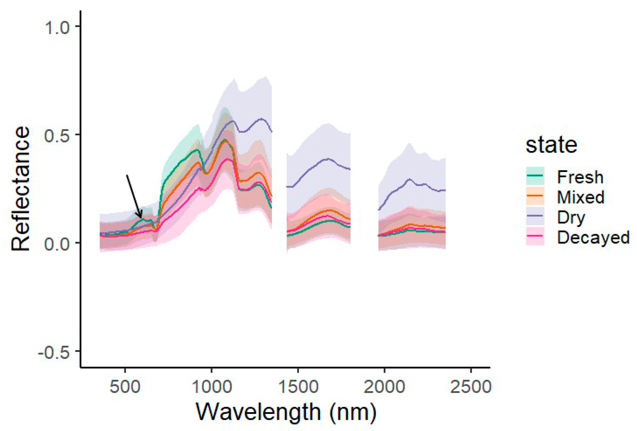
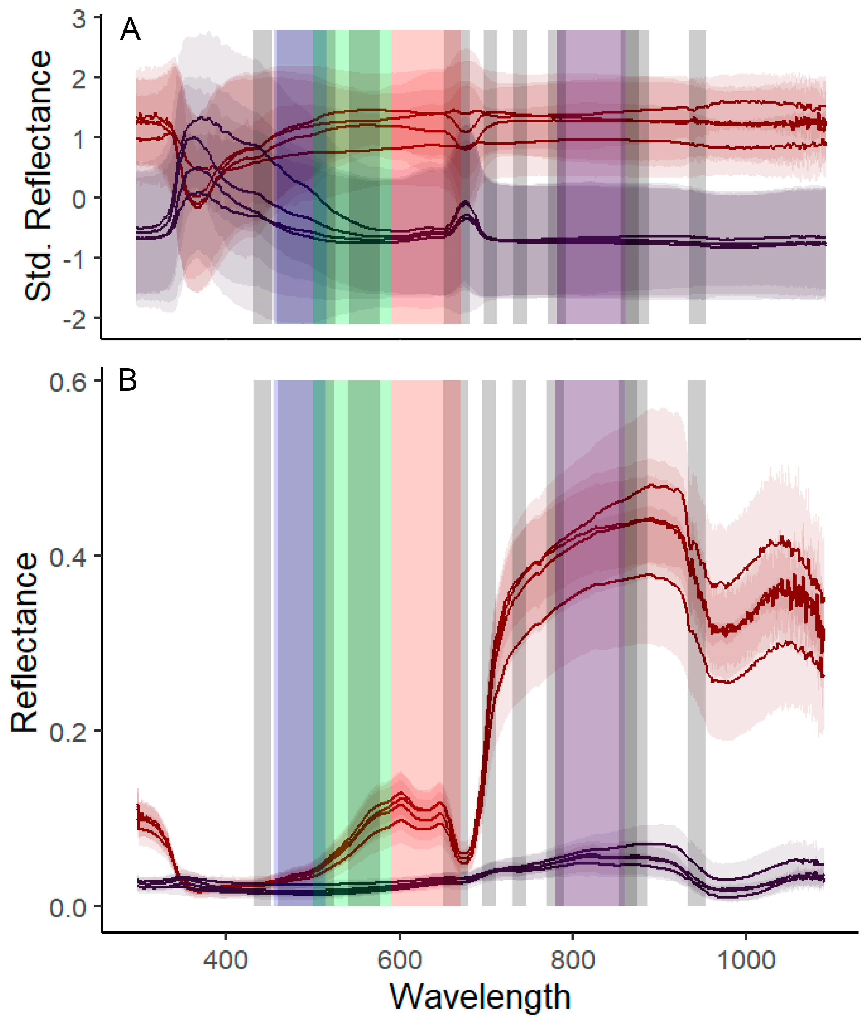
3.1. Spectral Response of Sargassum: Field Data

We found spectral differences between Sargassum in varying stages of freshness and decay. Fresh Sargassum exhibited a distinctive spectral response with two peaks in reflectance at 600 nm and 645 nm and a noticeable reflectance trough around 630 nm (i.e., chlorophyll C). As Sargassum dries or decays, the spectral response curve in the visible region changes considerably (Figure 3). In addition, while dried Sargassum showed a high reflectance in the near-infrared and shortwave-infrared regions in comparison to fresh material, the difference between the spectral reflectance of decayed and fresh material was less pronounced in the shortwave-infrared region (Figure 3).

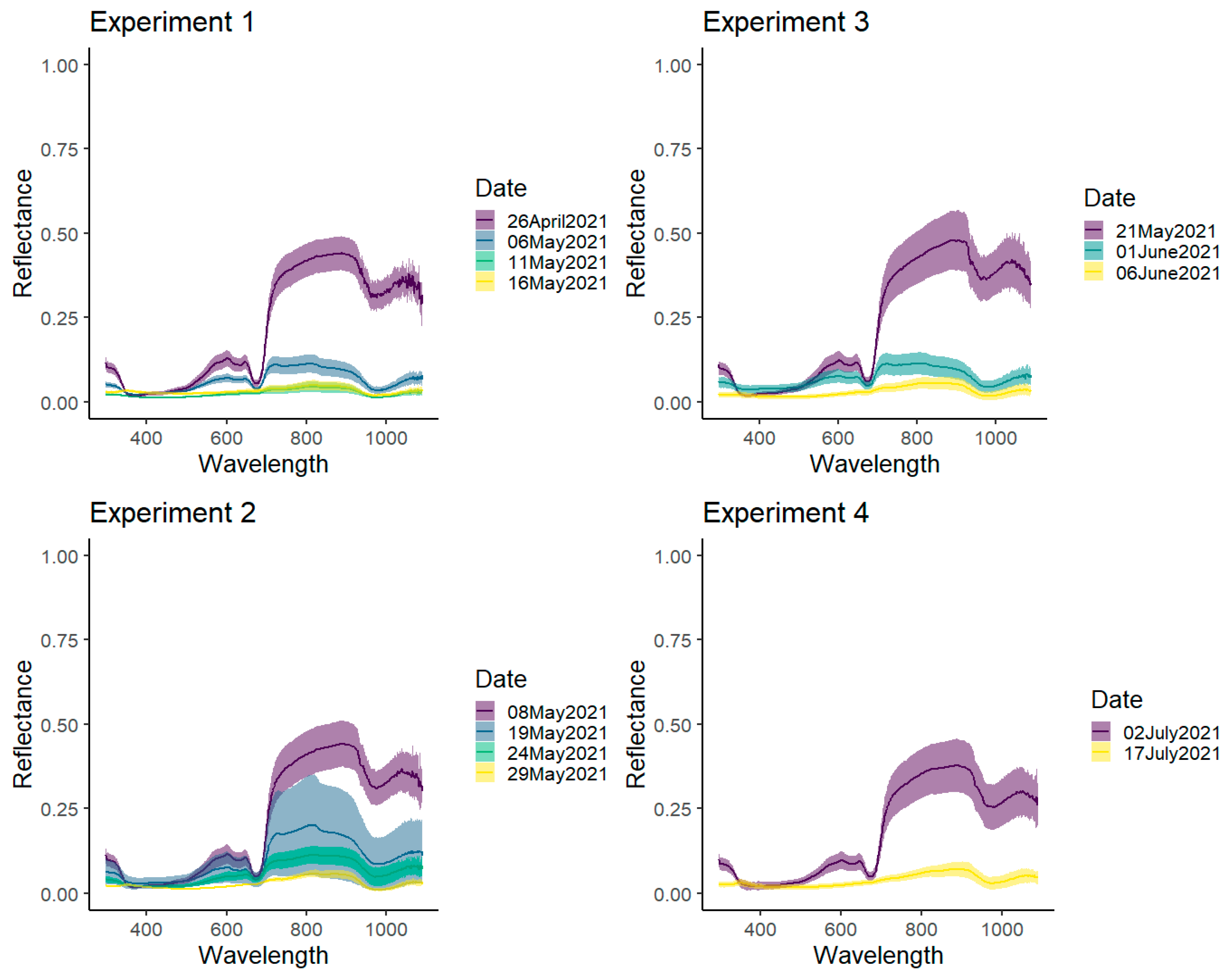
3.2. Spectral Response of Sargassum: Mesocosm Experiment

Spectral data collected from controlled mesocosm experiments revealed similar results to the spectral responses measured in the field. All four experiments showed the same distinctive reflectance curve (~600–645 nm) for the fresh material (Figure 4). A flattening of this curve, as well as an overall reduction in reflectance, was observed for the decayed material. Ten days after the start of the experiment, an overall decrease in reflectance was observed although the spectral shape remained. After 15 days from the start of the experiment, a flattening out of the spectra was observed.

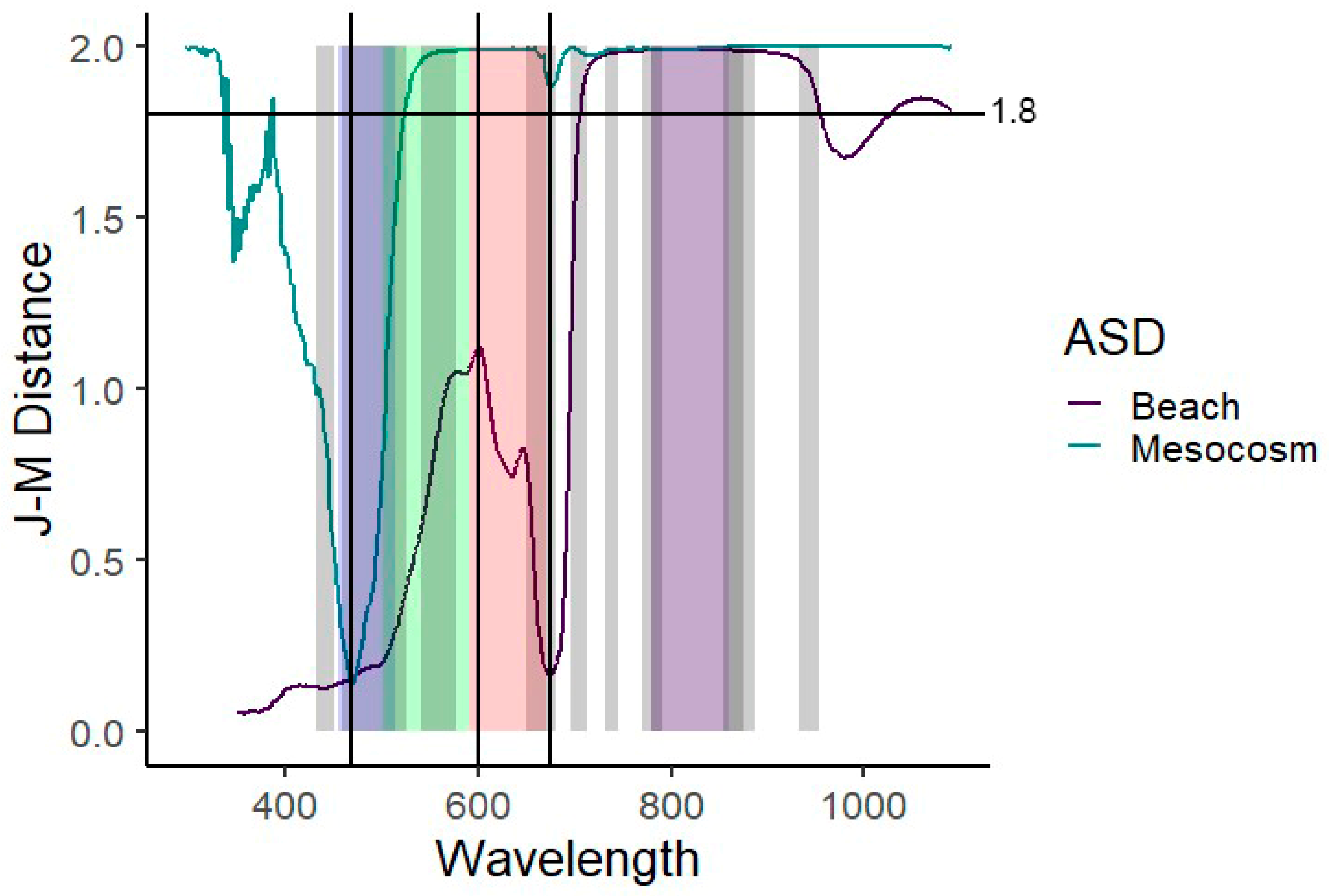
3.3. Regions of the Spectra That Offer the Greatest Separability

A change to the magnitude of reflectance, as well as the spectral shape, in response to decay demonstrates that remote sensing can be used to determine the state of Sargassum decay. All spectral bands (350–1050 nm) were evaluated to determine which regions offer the most potential for the separation of different states of Sargassum decay. The Jeffries–Matusita (J–M) distance revealed that all bands with an approximate wavelength of 540 nm or greater were likely to offer a similar degree of separability and resultant classification potential (Figure 5).
Results from the PCA also confirmed a clear separation between the fresh and decayed classes (Figure S2). This was also evident in the reflectance (Figure 6a) and standardised reflectance (Figure 6b), which showed greater separability between classes for wavelengths greater than ~540 nm. Standardised reflectance can more clearly show areas of greater separability as the magnitude of reflectance is removed such that relative differences in regions of the spectrum are more apparent. Standardised reflectance revealed a slightly greater separability between classes for wavelengths greater than ~690 nm as shown by a decrease in the overlap of standard deviations.

4. Discussion

Here, we show, for the first time, that there is a clear spectral contrast between fresh and decayed Sargassum. As Sargassum decays over time, a decrease in the magnitude of reflectance and a change to the spectral pattern are observed. Separability analyses suggest that most spectral bands greater than ~540 nm will be capable of discriminating between fresh and decayed material.
Two different methodologies were employed in order to assess spectral differences between fresh and decayed material. The spectral data from mesocosm experiments and that were recorded in situ revealed similar spectral differences between fresh and decayed Sargassum. This work therefore extends previous research that has focused on the detection of Sargassum and its discrimination from other vegetation [5,11,12,14].
A noticeable decrease in spectral reflectance for decayed Sargassum in contrast to fresh material was observed in the visible region (400–700 nm) due to a decrease in light absorption by the degraded pigments (Figure 6). For example, reflectance troughs at 630 nm and 670 nm have been linked to strong absorption by Chlorophyll (Chl)-c and Chl-a, respectively [30,31,32] (see also Figure 6). Pigments (Chl-a and Chl-b) absorb the majority of light in the blue-violet as well as the red wavelengths and this is evident from the local minima in the reflectance spectra between 350 nm and 450 nm for fresh Sargassum in comparison to decayed (Figure 3, Figure 4 and Figure 6). It is also known that as Chl pigments degrade, reflectance in the red region increases, producing a yellow senescent appearance. This difference is not observed in the spectral response of decayed material. However, an increase in red reflectance is observed for dry Sargassum in comparison to fresh (Figure 3). Further, a clear increase in reflectance across the near-infrared and shortwave-infrared regions (>1100 nm) is observed for dry Sargassum in comparison to fresh due to a decrease in the vegetation water content (Figure 3). Understanding the differences in the spectral reflectance of fresh and dry material [33] will be a useful step in order to achieve an accurate classification of fresh and decayed material.
Our analysis of the spectral differences between fresh and decayed Sargassum revealed that the majority of spectral bands are capable of discriminating between fresh and decayed material. The Jeffries–Matusita distance was used as a metric for separability whereby the degree of separability relates directly to the quality of a resultant classification. Separability was assessed for spectra collected in the mesocosm experiment and from material in situ on the beach. The results revealed the lower wavelengths (<540 nm) to have the lowest degree of separability and the near-infrared region to have the greatest degree of separability (Figure 5). Both methodologies showed similar reductions in separability at around 470 nm and 670 nm and greater separability around 600 nm and throughout the near-infrared region (Figure 5). In relation to the spectral regions of two different satellite-based sensors (Sentinel-2 and Planetscope), the band with lowest separability was limited to the blue region of the spectra (see Figure 5). A principal component analysis (PCA) was also conducted to support the results from the separability analysis. The contribution of spectral bands from the PCA output (Figure S3) also corroborated the results from the separability analysis, suggesting the blue region of the spectra is likely to be least effective, while all other bands may prove to be equally effective at discriminating between fresh and decayed spectra. This suggests that a machine learning approach may be the most appropriate method to capture variation across all spectral bands and achieve an accurate classification of fresh and decayed Sargassum. Machine learning approaches are also attractive for their ability to effectively manage mixed pixels in order to detect Sargassum at a sub-pixel scale [34,35,36].
The ability to accurately detect fresh and decayed Sargassum using satellite-based remote sensing will significantly improve our capability to predict the occurrence of decayed material and inform its targeted removal. While the spectra have revealed distinct differences between fresh and decayed material, results from the mesocosm experiment have also highlighted the length of time before fresh Sargassum begins to decay and the point at which this change is manifested in its spectral response. The early detection of decayed material will substantially improve efforts to control future beaching events. Clear differences in the spectral response of fresh Sargassum and Sargassum with early signs of decay (10–11 days after the experiment began) were observed. However, separability increased when fresh Sargassum was compared with Sargassum that had fully decayed over a 21-day period (Figure 4).
Our findings have demonstrated for the first time that there are distinct differences in the spectral characteristics of fresh and decayed Sargassum, suggesting that remote sensing technologies should be capable of accurately discriminating between fresh and decayed Sargassum. The use of remote sensing for the detection and management of Sargassum and other macroalgae has proven to be an effective tool [10,36,37,38,39,40,41,42,43,44,45]. However, in order to align ground observations of Sargassum distribution with satellite-derived imagery, large areas on the ground (greater than the size of pixels) are required in order to accurately classify different Sargassum states at the pixel level. The use of widely available multispectral sensors such as Sentinel-2 would therefore require large Sargassum patches in order to obtain a pixel with a good coverage of Sargassum. While the satellite-based detection of Sargassum would therefore underestimate the abundance of Sargassum, it would provide a tool to identify areas of large accumulation of both fresh and decaying masses over time. This would ultimately help to provide efficient and effective management of Sargassum at a landscape-level. Determining the location of large areas of fresh or decayed Sargassum will help to prioritise areas that require cleaning or where Sargassum can be harvested fresh for a range of purposes. Future work should focus on assessing the spatial and temporal units at which decayed Sargassum can be detected, and for which sensors offer the greatest potential for the effective detection and management of Sargassum. Future work should also look to collect a large dataset of satellite-derived spectral data relating to fresh and decayed Sargassum patches on the ground. A large dataset will be required in order to fulfil the training requirements of a machine learning approach. Data collection should also include the effect of the occurrence of other species of vegetation, such as sea grass [39,46,47,48], on the ability to accurately detect decayed Sargassum using remote sensing methods.

5. Conclusions

Characterising the spectral response of fresh and decayed Sargassum is a fundamental step in our ability to remotely detect decayed Sargassum and minimise its undesirable impacts. By utilising two different methodologies, we have demonstrated clear differences in the spectral responses of fresh and decayed Sargassum. We suggest that the near-infrared region may offer the greatest degree of separability for discriminating between fresh and decayed Sargassum. Subsequently, the use of multispectral sensors will likely be necessary to achieve a high classification accuracy. This study increases our understanding of the spectral characteristics of Sargassum and provides a first step in our ability to differentiate and detect fresh from decayed Sargassum. Being able to detect decayed Sargassum will provide a valuable tool for targeted beach cleaning action and effective management focused on Sargassum assessment and control.

Supplementary Materials

The following supporting information can be downloaded at: https://www.mdpi.com/article/10.3390/rs15174336/s1, Figure S1. Standard deviation of mean (n = 100) spectral reflectance against an increasing sample size; Figure S2. Spectral reflectance of Sargassum measured during sunny and cloudy conditions to determine the influence of weather conditions on the spectral responses.; Figure S3: Visualisation of the principal component analysis results showing the separation of spectral measurements from fresh and decayed Sargassum; Figure S4. The contribution of each spectral band to the first principal component showing a slight decrease at the lower wavelengths; Table S1. spectral measurements in different states.

Author Contributions

Conceptualisation, G.M.F. and B.d.l.B.-B.; methodology, C.J.C., G.M.F. and B.d.l.B.-B.; data collection, S.V.Á.-M., E.R.S.-A., E.M.-G., E.E.M. and M.A.G.R.; data analysis, C.J.C.; writing—C.J.C.; review and editing, C.J.C., S.V.Á.-M., E.R.S.-A., E.M.-G., E.E.M., M.A.G.R., B.d.l.B.-B., D.S.B., S.E.M., S.S., B.v.T., R.S. and G.M.F.; funding acquisition, G.M.F. All authors have read and agreed to the published version of the manuscript.

Funding

This research was funded by the UoN GCRF grant ‘Validation Sargassum detection’.

Data Availability Statement

Not applicable.

Acknowledgments

We acknowledge Jose Antonio Quintero and the Institute of Geography of UNAM for lending us a spectroradiometer for measuring the spectral data in the Mesocosms experiments, and José Antonio Lopez Portillo (SAMMO, UASA, UNAM) for logistic support. We acknowledge the Academic Meteorological and Oceanographic Monitoring Service (SAMMO) of the Reef Systems Academic Unit (UASA) from the Institute of Marine Sciences and Limnology (ICML) of the National Autonomous University of Mexico (UNAM).

Conflicts of Interest

The authors declare no conflict of interest.

References

  1. Ye, N.-H.; Zhang, X.-W.; Mao, Y.-Z.; Liang, C.-W.; Xu, D.; Zou, J.; Zhuang, Z.-M.; Wang, Q.-Y. ‘Green tides’ are overwhelming the coastline of our blue planet: Taking the world’s largest example. Ecol. Res. 2011, 26, 477–485. [Google Scholar] [CrossRef]
  2. Arroyo, N.L.; Aarnio, K.; Mäensivu, M.; Bonsdorff, E. Drifting filamentous algal mats disturb sediment fauna: Impacts on macro–meiofaunal interactions. J. Exp. Mar. Biol. Ecol. 2012, 420, 77–90. [Google Scholar] [CrossRef]
  3. Norkko, A.; Bonsdorff, E. Population responses of coastal zoobenthos to stress induced by drifting algal mats. Mar. Ecol. Prog. Ser. 1996, 140, 141–151. [Google Scholar] [CrossRef]
  4. Norkko, A.; Bonsdorff, E. Rapid zoobenthic community responses to accumulations of drifting algae. Mar. Ecol. Prog. Ser. 1996, 131, 143–157. [Google Scholar] [CrossRef]
  5. Gower, J.F.; King, S.A. Distribution of floating Sargassum in the Gulf of Mexico and the Atlantic Ocean mapped using MERIS. Int. J. Remote Sens. 2011, 32, 1917–1929. [Google Scholar] [CrossRef]
  6. Louime, C.; Fortune, J.; Gervais, G. Sargassum invasion of coastal environments: A growing concern. Am. J. Environ. Sci. 2017, 13, 58–64. [Google Scholar] [CrossRef]
  7. Schell, J.M.; Goodwin, D.S.; Siuda, A.N. Recent Sargassum inundation events in the Caribbean: Shipboard observations reveal dominance of a previously rare form. Oceanography 2015, 28, 8–11. [Google Scholar] [CrossRef]
  8. Chávez, V.; Uribe-Martínez, A.; Cuevas, E.; Rodríguez-Martínez, R.E.; Van Tussenbroek, B.I.; Francisco, V.; Estévez, M.; Celis, L.B.; Monroy-Velázquez, L.V.; Leal-Bautista, R. Massive influx of pelagic Sargassum spp. on the coasts of the Mexican Caribbean 2014–2020: Challenges and opportunities. Water 2020, 12, 2908. [Google Scholar] [CrossRef]
  9. Van Tussenbroek, B.I.; Arana, H.A.H.; Rodríguez-Martínez, R.E.; Espinoza-Avalos, J.; Canizales-Flores, H.M.; González-Godoy, C.E.; Barba-Santos, M.G.; Vega-Zepeda, A.; Collado-Vides, L. Severe impacts of brown tides caused by Sargassum spp. on near-shore Caribbean seagrass communities. Mar. Pollut. Bull. 2017, 122, 272–281. [Google Scholar] [CrossRef] [PubMed]
  10. Gower, J.; Hu, C.; Borstad, G.; King, S. Ocean color satellites show extensive lines of floating Sargassum in the Gulf of Mexico. IEEE TGRS 2006, 44, 3619–3625. [Google Scholar] [CrossRef]
  11. Hu, C.; Feng, L.; Hardy, R.F.; Hochberg, E.J. Spectral and spatial requirements of remote measurements of pelagic Sargassum macroalgae. Remote Sens. Environ. 2015, 167, 229–246. [Google Scholar] [CrossRef]
  12. Dierssen, H.; Chlus, A.; Russell, B. Hyperspectral discrimination of floating mats of seagrass wrack and the macroalgae Sargassum in coastal waters of Greater Florida Bay using airborne remote sensing. Remote Sens. Environ. 2015, 167, 247–258. [Google Scholar] [CrossRef]
  13. Gower, J.; Young, E.; King, S. Satellite images suggest a new Sargassum source region in 2011. Remote Sens. Lett. 2013, 4, 764–773. [Google Scholar] [CrossRef]
  14. Hu, C. A novel ocean color index to detect floating algae in the global oceans. Remote Sens. Environ. 2009, 113, 2118–2129. [Google Scholar] [CrossRef]
  15. Wang, M.; Hu, C. Predicting Sargassum blooms in the Caribbean Sea from MODIS observations. Geophys. Res. Lett. 2017, 44, 3265–3273. [Google Scholar] [CrossRef]
  16. Wang, M.; Hu, C.; Cannizzaro, J.; English, D.; Han, X.; Naar, D.; Lapointe, B.; Brewton, R.; Hernandez, F. Remote sensing of Sargassum biomass, nutrients, and pigments. Geophys. Res. Lett. 2018, 45, 12,359–12,367. [Google Scholar] [CrossRef]
  17. Uribe-Martínez, A.; Berriel-Bueno, D.; Chávez, V.; Cuevas, E.; Almeida, K.; Fontes, J.; van Tussenbroek, B.; Mariño-Tapia, I.; de los Ángeles Liceaga-Correa, M.; Ojeda, E. Multiscale distribution patterns of pelagic rafts of sargasso (Sargassum spp.) in the Mexican Caribbean (2014–2020). Front. Mar. Sci. 2022, 9, 920339. [Google Scholar] [CrossRef]
  18. Hinds, C.; Oxenford, H.; Cumberbatch, J.; Fardin, F.; Doyle, E.; Cashman, A. Golden Tides: Management Best Practices for Influxes of Sargassum in the Caribbean with a Focus on Clean-Up; Centre for Resource Management and Environmental Studies (CERMES), The University of the West Indies, Cave Hill Campus: Bridgetown, Barbados, 2016; p. 17. [Google Scholar]
  19. Robledo, D.; Vázquez-Delfín, E.; Freile-Pelegrín, Y.; Vásquez-Elizondo, R.M.; Qui-Minet, Z.N.; Salazar-Garibay, A. Challenges and opportunities in relation to Sargassum events along the Caribbean Sea. Front. Mar. Sci. 2021, 8, 699664. [Google Scholar] [CrossRef]
  20. López Miranda, J.L.; Celis, L.B.; Estévez, M.; Chávez, V.; van Tussenbroek, B.I.; Uribe-Martínez, A.; Cuevas, E.; Rosillo Pantoja, I.; Masia, L.; Cauich-Kantun, C. Commercial Potential of Pelagic Sargassum spp. in Mexico. Front. Mar. Sci. 2021, 8, 1692. [Google Scholar] [CrossRef]
  21. Kumar, Y.; Tarafdar, A.; Kumar, D.; Verma, K.; Aggarwal, M.; Badgujar, P.C. Evaluation of chemical, functional, spectral, and thermal characteristics of Sargassum wightii and ulva rigida from Indian Coast. J. Food Qual. 2021, 2021, 1–9. [Google Scholar] [CrossRef]
  22. Sembera, J.A.; Meier, E.J.; Waliczek, T.M. Composting as an alternative management strategy for sargassum drifts on coastlines. HortTechnology 2018, 28, 80–84. [Google Scholar] [CrossRef]
  23. León-Pérez, M.C.; Reisinger, A.S.; Gibeaut, J.C. Spatial-temporal dynamics of decaying stages of pelagic Sargassum spp. along shorelines in Puerto Rico using Google Earth Engine. Mar. Pollut. Bull. 2023, 188, 114715. [Google Scholar] [CrossRef]
  24. Coronado, C.; Candela, J.; Iglesias-Prieto, R.; Sheinbaum, J.; López, M.; Ocampo-Torres, F. On the circulation in the Puerto Morelos fringing reef lagoon. Coral Reefs 2007, 26, 149–163. [Google Scholar] [CrossRef]
  25. McHenry, J.; Rassweiler, A.; Hernan, G.; Uejio, C.K.; Pau, S.; Dubel, A.K.; Lester, S.E. Modelling the biodiversity enhancement value of seagrass beds. Divers. Distrib. 2021, 27, 2036–2049. [Google Scholar] [CrossRef]
  26. Sen, R.; Goswami, S.; Chakraborty, B. Jeffries-Matusita distance as a tool for feature selection. In Proceedings of the International Conference on Data Science and Engineering (ICDSE), Patna, India, 26–28 September 2019; pp. 15–20. [Google Scholar] [CrossRef]
  27. Evans, J.S.; Murphy, M.A. Spatialeco. R Package Version 2.0-1. 2021. Available online: https://github.com/jeffreyevans/spatialEco (accessed on 5 January 2023).
  28. R Core Team. R: A Language and Environment for Statistical Computing; R Foundation for Statistical Computing: Vienna, Austria, 2021; Available online: https://www.R-project.org/ (accessed on 15 January 2023).
  29. Kassambara, A.; Mundt, F. Factoextra: Extract and Visualize the Results of Multivariate Data Analyses. R Package Version 1.0.7. 2020. Available online: https://CRAN.R-project.org/package=factoextra (accessed on 7 February 2023).
  30. Beach, K.; Borgeas, H.; Nishimura, N.; Smith, C. In vivo absorbance spectra and the ecophysiology of reef macroalgae. Coral Reefs 1997, 16, 21–28. [Google Scholar] [CrossRef]
  31. Bricaud, A.; Claustre, H.; Ras, J.; Oubelkheir, K. Natural variability of phytoplanktonic absorption in oceanic waters: Influence of the size structure of algal populations. J. Geophys. Res. Oceans 2004, 109, C11. [Google Scholar] [CrossRef]
  32. Orzymski, J.; Johnsen, G.; Sakshaug, E. The significance of intracellular self-shading on the biooptical properties of brown, red, and green macroalgae 1. J. Phycol. 1997, 33, 408–414. [Google Scholar] [CrossRef]
  33. Chandler, C.J.; Wilts, B.D.; Vignolini, S.; Brodie, J.; Steiner, U.; Rudall, P.J.; Glover, B.J.; Gregory, T.; Walker, R.H. Structural colour in Chondrus crispus. Sci. Rep. 2015, 5, 11645. [Google Scholar] [CrossRef]
  34. Foody, G.M.; Lucas, R.; Curran, P.; Honzak, M. Non-linear mixture modelling without end-members using an artificial neural network. Int. J. Remote Sens. 1997, 18, 937–953. [Google Scholar] [CrossRef]
  35. Foody, G.M.; Mathur, A. The use of small training sets containing mixed pixels for accurate hard image classification: Training on mixed spectral responses for classification by a SVM. Remote Sens. Environ. 2006, 103, 179–189. [Google Scholar] [CrossRef]
  36. Li, L.; Zheng, X.; Wei, Z.; Zou, J.; Xing, Q. A spectral-mixing model for estimating sub-pixel coverage of sea-surface floating macroalgae. Atmos. Ocean 2018, 56, 296–302. [Google Scholar] [CrossRef]
  37. Brodie, J.; Ash, L.V.; Tittley, I.; Yesson, C. A comparison of multispectral aerial and satellite imagery for mapping intertidal seaweed communities. Aquat. Conserv. 2018, 28, 872–881. [Google Scholar] [CrossRef]
  38. Rossiter, T.; Furey, T.; McCarthy, T.; Stengel, D.B. Application of multiplatform, multispectral remote sensors for mapping intertidal macroalgae: A comparative approach. Aquat. Conserv. 2020, 30, 1595–1612. [Google Scholar] [CrossRef]
  39. Bakirman, T.; Gumusay, M.; Tuney, I. Mapping of the seagrass cover along the Mediterranean coast of Turkey using Landsat 8 OLI images. ISPRS 2016, 8, 1103–1105. [Google Scholar]
  40. Chen, Y.-L.; Wan, J.-H.; Zhang, J.; Ma, Y.-J.; Wang, L.; Zhao, J.-H.; Wang, Z.-Z. Spatial-temporal distribution of golden tide based on high-resolution satellite remote sensing in the South Yellow Sea. J. Coast. Res. 2019, 90, 221–227. [Google Scholar] [CrossRef]
  41. Hu, C.; Cannizzaro, J.; Carder, K.L.; Muller-Karger, F.E.; Hardy, R. Remote detection of Trichodesmium blooms in optically complex coastal waters: Examples with MODIS full-spectral data. Remote Sens. Environ. 2010, 114, 2048–2058. [Google Scholar] [CrossRef]
  42. Huang, X.; Wang, D.; Bao, M.; Gong, F.; Bai, Y. Spectral characteristics of Sargassum horneri in seawater. In Proceedings of the SPIE 10850, Ocean Optics and Information Technology, Beijing, China, 22–24 May 2018; pp. 269–275. [Google Scholar] [CrossRef]
  43. Pan, X.; Meng, D.; Ren, P.; Xiao, Y.; Kim, K.; Mu, B.; Tao, X.; Liu, R.; Wang, Q.; Ryu, J.-H. Macroalgae monitoring from satellite optical images using Context-sensitive level set (CSLS) model. Ecol. Indic. 2023, 149, 110160. [Google Scholar] [CrossRef]
  44. Qi, L.; Hu, C. To what extent can Ulva and Sargassum be detected and separated in satellite imagery? Harmful Algae 2021, 103, 102001. [Google Scholar] [CrossRef]
  45. Setyawidati, N.; Kaimuddin, A.H.; Wati, I.; Helmi, M.; Widowati, I.; Rossi, N.; Liabot, P.; Stiger-Pouvreau, V. Percentage cover, biomass, distribution, and potential habitat mapping of natural macroalgae, based on high-resolution satellite data and in situ monitoring, at Libukang Island, Malasoro Bay, Indonesia. J. Appl. Phycol. 2018, 30, 159–171. [Google Scholar] [CrossRef]
  46. Orth, R.J.; Carruthers, T.J.; Dennison, W.C.; Duarte, C.M.; Fourqurean, J.W.; Heck, K.L.; Hughes, A.R.; Kendrick, G.A.; Kenworthy, W.J.; Olyarnik, S. A global crisis for seagrass ecosystems. J. Biosci. 2006, 56, 987–996. [Google Scholar] [CrossRef]
  47. Pergent, G.; Bazairi, H.; Bianchi, C.N.; Boudouresque, C.F.; Buia, M.; Calvo, S.; Clabaut, P.; Harmelin-Vivien, M.; Mateo, M.A.; Montefalcone, M. Climate change and Mediterranean seagrass meadows: A synopsis for environmental managers. Mediterr. Mar. Sci. 2014, 15, 462–473. [Google Scholar] [CrossRef]
  48. Riani, E.; Djuwita, I.; Budiharsono, S.; Purbayanto, A.; Asmus, H. Challenging for seagrass management in Indonesia. J. Coast. Dev. 2012, 15, 234–242. [Google Scholar]
Figure 1. (A) Sargassum data collection sites near Puerto Morelos, (B) photograph showing an example of a sampling location and (C) the location of the study area.
Remotesensing 15 04336 g001
Figure 2. Standard deviation of mean spectral reflectance against an increasing sample size for Sargassum in three different states: dry, fresh and mixed (dry and fresh).
Remotesensing 15 04336 g002
Figure 3. Spectral reflectance of Sargassum for the four states observed. The lines represent mean reflectance values for fresh (n = 531), mixed (n = 430), dry (n = 680) and decayed (n = 228) (shading ± 1 SD). Black arrow indicates the region where a noticeable difference in the spectral response is observed between fresh vs. dry or decayed Sargassum.
Remotesensing 15 04336 g003
Figure 4. Spectral reflectance of Sargassum sp. obtained from mesocosm experiments over time across wavelength range 350–1050 nm. Experiments were controlled at varied temperatures. Experiment 1: 22 °C, Experiment 2: 25 °C, Experiment 3: 28 °C and Experiment 4: 31 °C. Lines are mean reflectance values (shading ± 1 SD) for Sargassum (n = 30) ranging from fresh (purple) to dry (yellow).
Remotesensing 15 04336 g004
Figure 5. The Jeffries–Matusita (J–M) distance, as a function of separability, between the spectral reflectance of fresh (n = 50) and decayed (n = 50) Sargassum. The lines represent the J–M distance for Sargassum collected by the analytical spectral device (ASD) in situ on the beach (beach: shown in purple) as well as in mesocosm experiments (mesocosm: shown in green) across a wavelength range of 350–1050 nm. The coloured vertical bars represent the wavelength regions for Planet Scope and the grey vertical bars represent the wavelength regions for Sentinel-2. Black vertical lines correspond to regions of reduced (470 nm and 670 nm) and increased (600 nm) separability and the black horizonal line corresponds to a J–M distance of 1.8.
Remotesensing 15 04336 g005
Figure 6. Spectral reflectance (A) and standardised reflectance (B) for fresh and decayed Sargassum. Lines are mean reflectance values for fresh (red) and decayed (blue) Sargassum (shading ± 1 SD). Coloured vertical bars represent the spectral regions for Planet Scope and grey vertical bars represent the spectral regions for Sentinel-2.
Remotesensing 15 04336 g006
Disclaimer/Publisher’s Note: The statements, opinions and data contained in all publications are solely those of the individual author(s) and contributor(s) and not of MDPI and/or the editor(s). MDPI and/or the editor(s) disclaim responsibility for any injury to people or property resulting from any ideas, methods, instructions or products referred to in the content.

