
An Algorithm for Building Exterior Facade Corner Point Extraction Based on UAV Images and Point Clouds


School of Environmental Science and Spatial Informatics, China University of Mining and Technology, Xuzhou 221116, China
*
Author to whom correspondence should be addressed.
Remote Sens. 2023, 15(17), 4166; https://doi.org/10.3390/rs15174166
Submission received: 11 July 2023
/
Revised: 18 August 2023
/
Accepted: 21 August 2023
/
Published: 24 August 2023
(This article belongs to the Section Engineering Remote Sensing)
Abstract
:The high-precision building exterior facade corner point (BEFCP) is an essential element in topographic and cadastral surveys. However, current extraction methods rely on the interactions of humans with the 3D real-scene models produced by unmanned aerial vehicle (UAV) oblique photogrammetry, which have a high workload, low efficiency, poor precision, and cannot satisfy the requirements of automation. The dense point cloud contains discrete 3D building structure information. Still, it is challenging to accurately filter out the partial point cloud characterizing the building structure from it in order to achieve BEFCP extraction. The BEFCPs are always located on the plumb line of the building’s exterior wall. Thus, this paper back-calculated the plumb line from the image and designed a photographic ray corresponding to the image point and point cloud intersection point calculation algorithm to recover its approximate spatial position in order to successfully extract the accurate point cloud in the building structure neighborhood. It then utilized the high signal-to-noise ratio property of the point cloud as a base to eliminate the noise points and, finally, accurately located the building exterior façade corner points by recovering the building structure through segmental linear fitting of the point cloud. The proposed algorithm conducted automated building exterior facade corner point extraction via both of planar-to-stereo and rough-to-precise strategies, reached a 92.06% correctness rate and ±4.5 cm point mean square location error in the experiment, and was able to extract and distinguish the building exterior facade corner points under eaves obstruction and extreme proximity. It is suitable for all high-precision surveying and mapping tasks in building areas based on oblique photogrammetry, which can effectively improve the automation of mapping production.
1. Introduction
Buildings are the most valuable features in the geographic database, which is frequently changing. There are high accuracy requirements for measuring buildings in many surveying and mapping production tasks, such as large-scale topographic maps, cadastral surveys, and real estate mapping. The vector contour points of buildings are composed of the contour corner of the building’s exterior facade (as shown in Figure 1) rather than the corners of the building’s footprint. The acquisition method of BEFCPs still relies on fieldwork using an electronic total station, with low automation. In recent years, it has been gradually replaced by oblique photogrammetry. Research on the automatic extraction algorithm of BEFCPs with high accuracy and generalization can effectively improve the automation of production tasks with high accuracy requirements and promote the development of intelligent mapping.
Building extraction has been one of the research focuses of Earth observation techniques. However, buildings show complex and individual textures and heterogeneous and diverse contours in regions affected by the environment and culture, making exploring universal high-precision building extraction algorithms challenging. Much research has been carried out on 2D and 3D building contour extraction.
Segmenting buildings via the Digital Orthophoto Map (DOM) or Digital Surface Model (DSM) and then performing contour fitting are the common 2D building contour extraction methods.
Methods based on pixel features such as spectral, texture, etc., or based on deep learning are the common methods to realize building segmentation. Liasis and Stavrou [1] analyzed the images’ RGB and HSV color attributes and optimized the extracted buildings via the active contour segmentation framework. Avudaiammal et al. [2] combined morphological, spectral, and other features using the support vector machine (SVM) classifier to extract the roofs of buildings from images. Zhang et al. [3] simultaneously used spatial information from DSM and spectral information from DOM to extract geometric building information, and the maximum average relative error of the extracted building area was less than 8%. Semantic segmentation algorithms in deep learning are often applied in order to extract buildings. Maltezos et al. [4] designed convolutional neural networks to extract buildings using the DSM, DOM, and normalized difference vegetation index (NDVI) as inputs. Shi et al. [5] designed a control graph convolutional network to segment the building footprint. Li et al. [6] utilized U-Net in order to segment buildings from satellite imagery and corrected the results using the multi-source map dataset. Pan et al. [7] segmented images with superpixels as input units to solve the problem that convolutional neural networks (CNNs) require rectangle inputs, then obtained semantic segmentation results for objects such as buildings and low vegetation.
The contour fitting of buildings is generally achieved via corner point localization or regular contour methods. The former firstly extracts the corner points of the buildings and then connects them in sequence to obtain the building contours. The latter is based on the buildings’ regularity, determining the main direction and then adjusting the other contour lines to reconstruct the building contours.
Harris [8], Susan [9], ORB [10], etc., are suitable corner detection algorithms for buildings [11,12,13]. Li et al. [14] used the Harris operator to obtain the edge point set of buildings and identified the building corner points based on support vector machine (SVM). Wang et al. [15] used the Harris and Susan operators, respectively, to detect and extract the building corner points and used least squares fitting to fit the building contours after sorting. Cui et al. [16] used the two groups of vertical lines geometry corresponding to the building boundaries obtained via Hough linear detection. They reconstructed the regular building contours using the nodes of the two line segment sets. Turker and Koc-San [17] obtained the building boundaries using perceptual grouping line detection and reconstructed the square building contours. Partovi et al. [18] determined the main direction using the length and arc length of the building line segments. They formed polygons representing the building contours by aligning and adjusting the line segments according to the main direction of the buildings through a regularization process.
However, the 2D building footprint obtained based on DOM or DSM is the outer contour represented by the roof edge but not the exterior contour corner of the main structure, which cannot be applied to mapping production tasks such as large-scale topographic maps, cadastral surveys, etc.
Three-dimensional building models are generally extracted from multi-view images of oblique photography or dense point clouds.
Extracting 3D buildings from multi-view images is an effective method based on oblique photogrammetry. Xiao et al. [19] extracted 3D lines from multi-view images and combined them with building geometry features to extract building structures that reach a 0.2 m height accuracy. Xiao et al. [20] used oblique images taken in the same direction to detect the facade and applied box model matching to extract a building with a positioning accuracy of 0.25 m. However, both of the above methods are only suitable for simple buildings with rectangular structures. Zhuo et al. [21] obtained building contours using semantic segmentation of UAV tilt images and employed them to optimize the spatial information of 3D buildings in OpenStreetMap (OSM), where the footprint accuracy reaches the decimeter level. Still, the method is not applicable to regions obscured by trees or other buildings.
The dense point cloud contains intuitive 3D spatial information, which is the most common data for 3D building extraction. Nex et al. [22] detected and reconstructed building footprints via morphological filtering, skeletonization, and smoothing of facade points in dense point clouds. However, the wall’s continuity was affected by the shading of trees or adjacent buildings, and extracted edges were loose and needed to be generalized and modeled before application. Acar et al. [23] automatically extracted vegetation and building roofs using dense point clouds obtained from the matching of high-resolution infrared images, then obtained high-quality results using LiDAR data. Extracting contours from point clouds and performing cluster analysis is another approach for building contour extraction [24,25,26]. Such methods layer the point clouds by height, then fit the contours of each layer, and finally combine them to generate a building model. The method based on dense point clouds cannot utilize the texture features, and it is generally hard to reconstruct buildings with complex structures. The accuracy is limited to the decimeter level.
As shown in Figure 1, the BEFCP provides more accurate spatial location information than the building footprint, becoming an essential element in topographic and cadastral surveys. In mapping tasks that require high accuracy of houses, the building contours measured are composed of BEFCPs. BEFCPs cannot be obtained from DOM or DSM, and data such as multi-view oblique images and dense point clouds that contain 3D structure information of buildings are the data basis for BEFCP production.
Currently, low-altitude UAV oblique photography is an effective way to produce mapping data. The images preserve the tight and smooth textural features, and the different shooting views additionally enhance the building facades’ linear features. Meanwhile, the point cloud derived from dense matching combines the homonymous points of each image. The point cloud has a large number of points in it, preserving discrete but complete 3D structural information, losing the smoothing features but balancing the accuracy.
Accurately retrieving the point cloud representing BEFCPs is the key to locating BEFCPs. Existing algorithms typically separately adopt images or dense point clouds. However, images lose intuitive 3D information, and dense point clouds lack tight texture. The information of the identified object cannot be fully integrated and utilized, making it very difficult to locate spatial data that accurately represent BEFCPs. The BEFCP is represented as a line and a discrete point set with certain rules in images and point clouds, respectively. Hence, it’s a feasible approach to extract the BEFCP by combining the advantages of images and high-density point clouds.
In summary, based on the relevant data produced by UAV oblique photogrammetry, this paper extracts the line segments where the BEFCP is located from the images and uses the collinearity of the image point and object point as the link; accurately extracts the discrete points representing BEFCPs from the point clouds; and realizes the automatic extraction of BEFCPs.
2. Methodology
The BEFCP is the projection of the building exterior facade plumb line on the horizontal plane. And the plumb line is the line connecting the object’s gravity center with the Earth’s gravity center, which is widely used in measurement, building construction, aerospace, etc. The dense point cloud preserves discrete 3D structural information. Extracting an accurate partial point cloud characterizing the building structure is crucial to achieving BEFCP identification and localization.
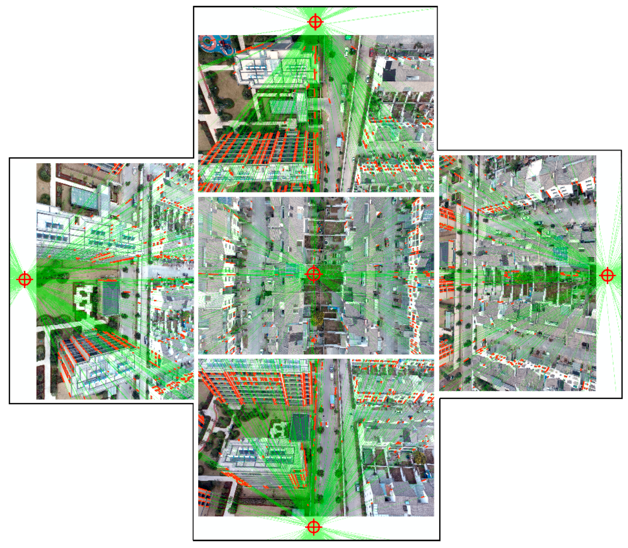
The spatial line segment in the image maintains tight and complete geometric line features. Low-altitude UAV oblique photography is the central projection method, and the plumb line extension represented by the building’s facade outline intersects at the photo nadir point (as shown in Figure 2). This property can be utilized for the initial back-calculation of plumb lines in the image, providing the search index to extract partial point clouds characterizing the building structure. The algorithm flow is shown in Figure 3.
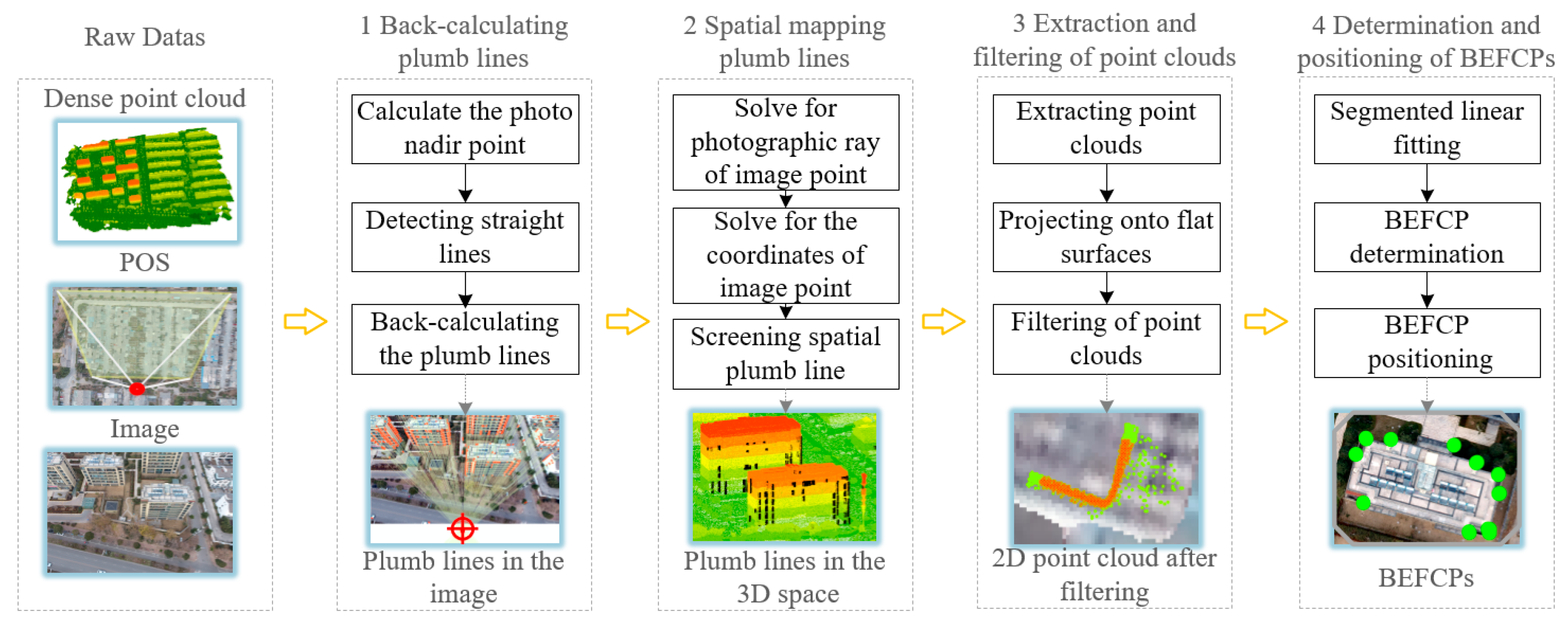
The proposed algorithm consists of four main steps. Firstly, the photo nadir point is calculated using the camera position and back-calculating the plumb lines in the image. Secondly, a photographic ray and dense point cloud intersection point calculation algorithm is implemented based on the camera perspective model to map plumb lines in the image to spatial. Then, point clouds are screened using the spatial position and elevation of the plumb line, and a point cloud filtering algorithm with a dynamic radius is designed to eliminate the discrete points resulting from the roofs, trees, etc., to obtain the filtered point cloud for determining the BEFCP. Finally, segmented linear fitting is applied to extract the structure lines of the building represented by the filtered point cloud and finally achieve the accurate determination and high-precision positioning of the BEFCP.
The algorithm is implemented in C# language based on the Visual Studio 2019 platform. OpenCV implements image-related operations such as image filtering, line detection, etc., and spatial query functions such as point cloud retrieval are completed by Esri’s ArcObjects 10.2.
2.1. Plumb Line Back-Calculation Based on Photo Nadir Point
2.1.1. Calculation of Photo Nadir Point
The photo nadir point is the intersection of the image plane and the plumb line through the projection center, and its pixel coordinate is not related to the position elements of the exterior orientation but only to the angle. After the aerotriangulation of the oblique photogrammetry task is completed, the camera’s intrinsic and extrinsic elements can be obtained, and the pixel coordinate of the photo nadir point can be calculated using Equation (1).
where is the camera’s focal length, and , , and are the heading, lateral, and photo tilt angle in the ground-assisted coordinate system with the x-axis as the heading direction, respectively.
2.1.2. Extraction of Line
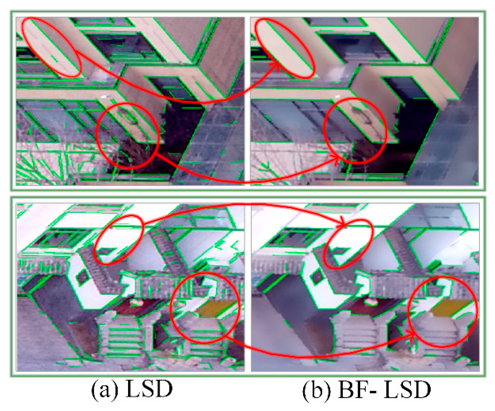
The resolution of low-altitude UAV images reaches the centimeter level, with high-definition details, while bringing lots of noise to the extract targets. Bilateral filtering (BF) combines the image’s spatial proximity and pixel similarity, considering the neighborhood and grayscale information. It can preserve edge-specific features, such as the outer contours of buildings, while removing internal texture noise, such as brickwork, grass, and trees. Line segment detector (LSD) [27] was adopted to detect the line segments in the image after BF. The building feature lines were retained while effectively reducing the noise edges from the internal texture, as shown in the green lines in red circles in Figure 4.
2.1.3. Determination of Plumb Line
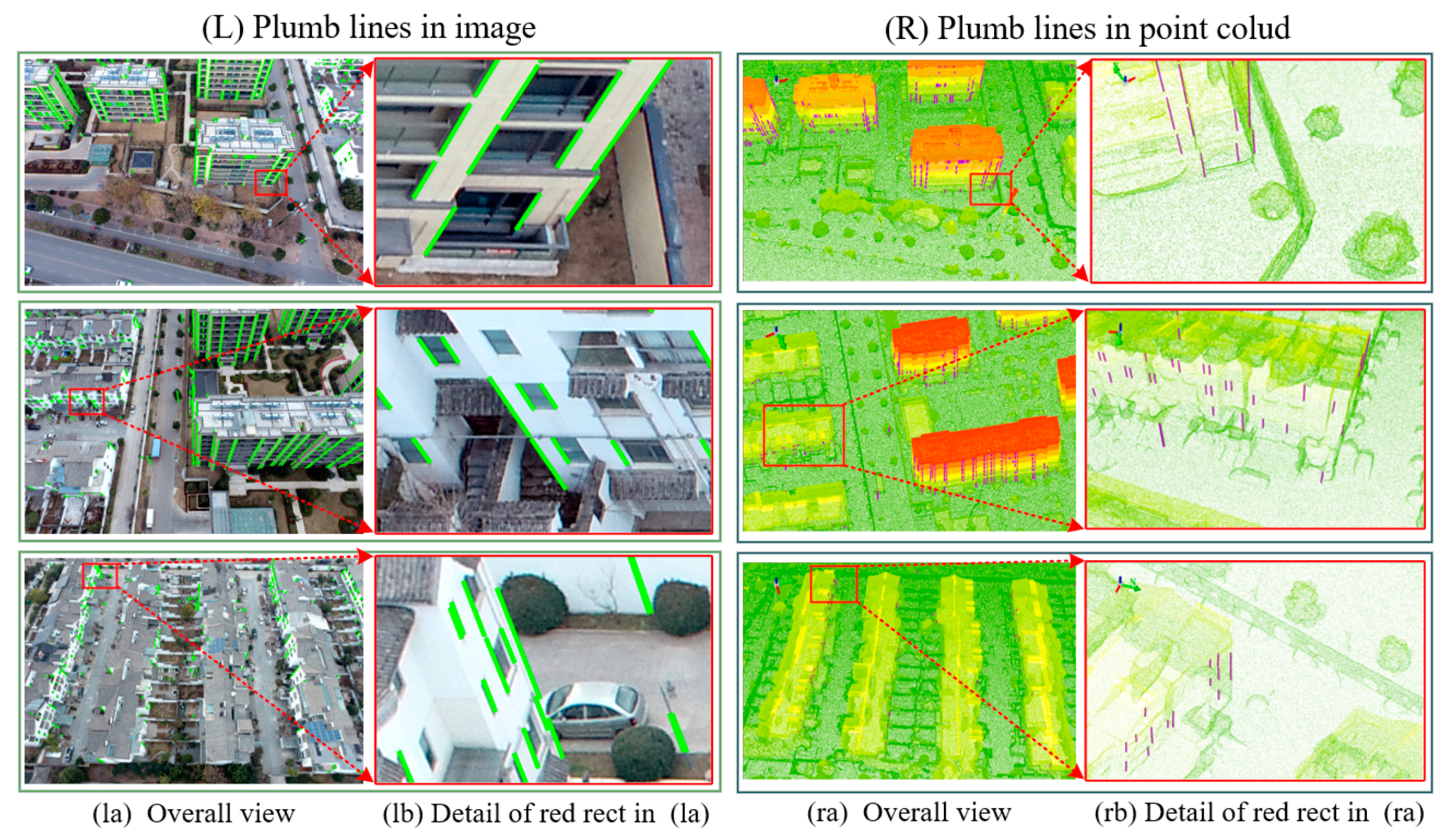
The plumb line does not strictly intersect the photo nadir point, manifested by the angle deviation between the extension of the line segment and the photo nadir point or the distance deviation from the photo nadir point to the line segment. It is difficult to correctly distinguish the plumb line from other line segments using distance deviation when the photo nadir point is located inside the image because part of the line segment is near the photo nadir point. Therefore, the deviation angle was adopted as the criterion for the determination of the plumb line, where and are the endpoints of the image segment, is the photo nadir point, and when is less than the specified threshold (3° in this paper), the current segment is regarded as a plumb line. Figure 5L shows the screening results of the plumb lines in parts of the images in the experiment, and the main plumb structures of the building dominated by the wall corners are extracted.
2.2. Spatial Mapping of the Plumb Line
However, the plumb line and the BEFCP don’t completely correspond to each other, and the spatial position and structure are hard to be determined from a single image. The next step is to transform the plumb line from image coordinates to space through the camera perspective model to extract the neighborhood point cloud and further characterize it via spatial analysis.
2.2.1. Calculation of Photographic Ray of the Image Point
The solution of the image point to the world coordinate system’s homonymous object point is manifested as a photographic ray through the photographic center in space. The camera perspective model converts the object point coordinates from the world space to the image space by homogeneous coordinate transformation, and the inverse process can obtain the photographic ray corresponding to the image point.
2.2.2. Object Point Coordinate Calculation Corresponding to the Image Point
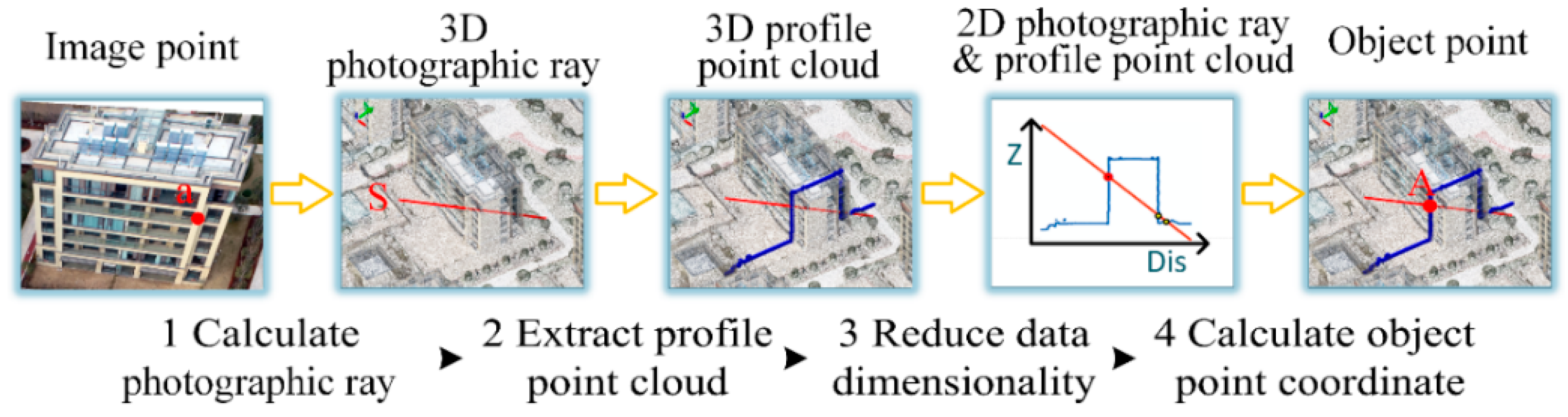
As shown in Figure 6, the coordinate of the object point corresponding to the image point is calculated by intersecting the photographic ray of the image point with the dense point cloud.
Firstly, use the inverse process of the camera perspective model to calculate the photographic ray of the homonymous object point corresponding to the image point.
Secondly, after projecting the photographic ray onto the plane, extract the 3D profile point cloud within its certain buffer range (0.015 m in this paper) from the dense point cloud.
Then, reduce the dimensionality of and . Redefine the 2D coordinate axes, where the horizontal axis is the plane distance from the 3D point to the starting point; the vertical axis is the original elevation value of the 3D point used to obtain the 2D photographic ray and the 2D profile point cloud set .
Finally, interpolate the ground 3D coordinates corresponding to the image point using and . Calculate the distance from the points in to and pick out the nearest partial points from (12 points in this paper). Classify the points in as either above or below to generate the point sets and , respectively. Join the points in and one by one to create the 2D line segment set . Retaining the lines in , intersect them with as the possible profile line segment set . Calculate the intersection of the line segments in with to obtain the intersection point set . Higher objects are always observed first in the aerial view, so the maximum value in is taken to be the elevation value corresponding to the ground point. The 3D coordinate of the ground point corresponding to the image point is obtained by truncating the at .
2.2.3. Spatial Plumb Line Screening
The line segments passing through the photo nadir point are not always plumb lines. The 3D coordinates of the line segment endpoints extracted from the image were calculated to obtain the 3D line segment. Its deviation angle τ with the plumb line was calculated. The spatial line segment in which is less than the specified threshold (3° in this paper) was selected as the plumb line. The plumb line was regarded as the accurate spatial 3D index to extract the point cloud to determine and position BEFCPs. Figure 5R shows the spatial plumb line screening results corresponding to Figure 5L.
The spatial plumb line can be employed as the spatial search domain index to accurately extract 3D point clouds of building contours for BEFCP determination and high-precision positioning.
2.3. Extraction and Filtering of Point Clouds
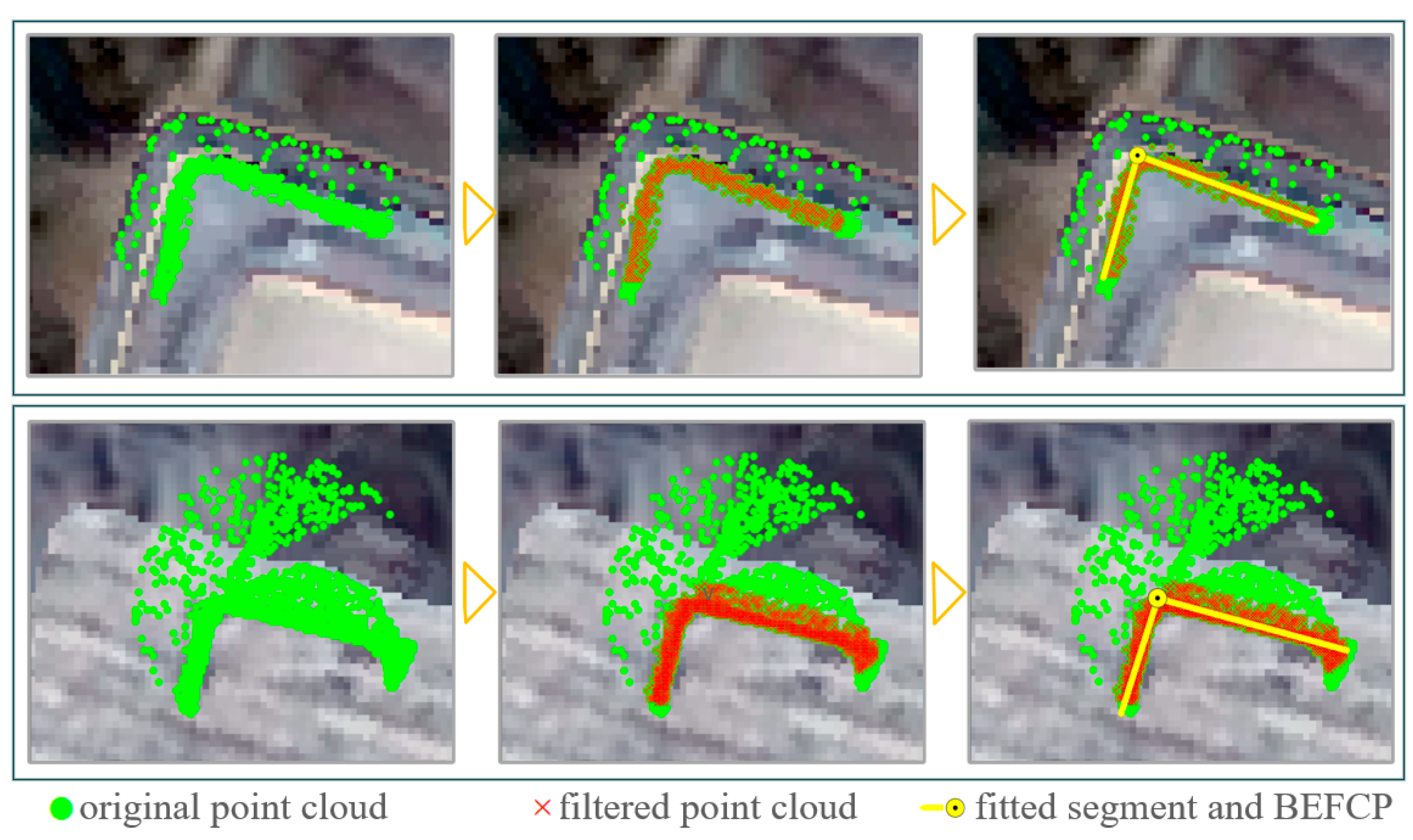
The elevation range of the spatial plumb line and the buffer zone of its ground projection is employed as the point cloud’s elevation and plane search domain (the buffer radius is taken as 0.3 m in this paper). The original point cloud used for BEFCP determination (shown as green points in Figure 7) contains discrete noises from mismatched or non-wall points consisting mainly of roofs and adjacent vegetation, which need to be filtered before fitting.
Benefiting from the precise spatial constraints assigned by the spatial plumb line, the target points’ number in original point clouds is significantly more than noise points and has the spatial characteristic of distribution along the building facade. Based on these two properties, the radius point cloud filtering algorithm rejected the error points after downscaling the original point cloud to the XY plane.
After the original point cloud is projected onto the XY plane, the computational cost of the point filtering is reduced, and the spatial aggregation of target points is enhanced. The point cloud filtering algorithm first counts the proximity point numbers within a certain radius (0.1 m in this paper) of each point and identifies points with fewer proximity point numbers (the lesser 20% is taken in this paper) as noise and rejects them; the 2D filtered point cloud for BEFCP determination is finally generated. The red points in Figure 7 are examples of the point clouds for structure determination derived from the original point cloud after dimensionality reduction and filtering.
2.4. Determination and Locating of BEFCP
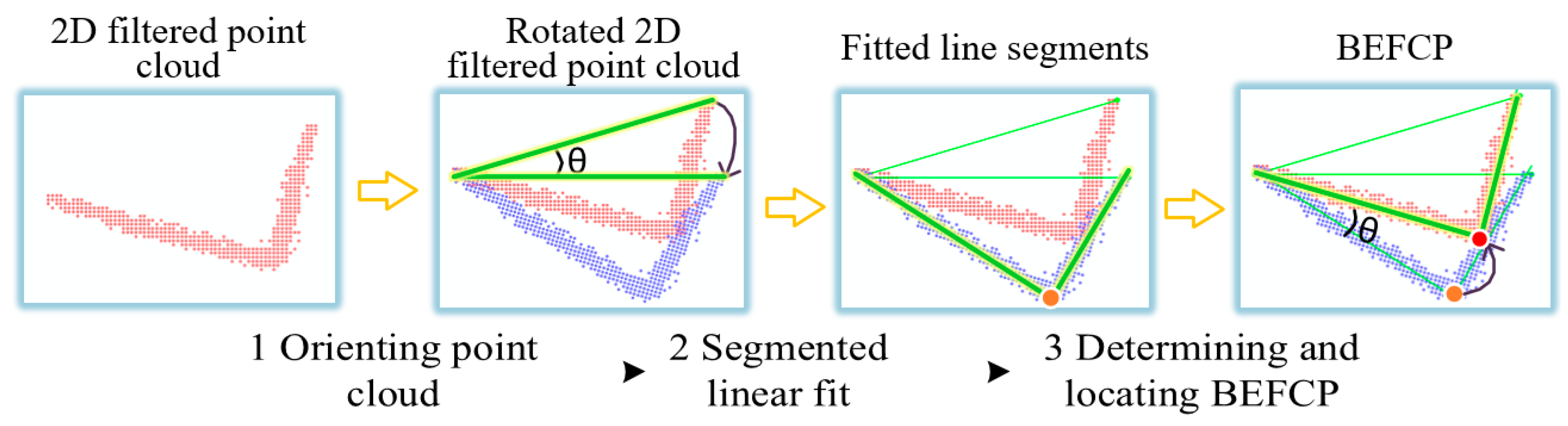
A BEFCP is located on the intersection line of the two building facades, and the 2D filtered point cloud contains its discrete spatial structure information. Therefore, the building structure was determined via the segmented linear fitting of distribution. And the intersection point of the fitted line segments is adopted as the precision coordinates of the BEFCP. The flow chart is shown in Figure 8.
Firstly, point cloud orientation is performed to ensure that the point cloud is fitted with segmented linear fitting in the x-axis direction. Take the coordinate center of as the origin and the x-axis and y-axis as the division lines to divide the point cloud into four pieces, calculate the distance between two pieces of the point cloud, and obtain the farthest two points as the point cloud direction axis . Then, calculate the angle between and the x-axis. At last, rotate and clockwise by with the left point of as the rotation center to obtain the and the point cloud .
Then, fit the distribution of using a segmented linear function to obtain the characteristic line segments representing the building structure. First, calculate the point farthest from in to locate the approximate position of the segmentation point. Then, calculate the thickness of the point cloud to determine the search range of the segmented points. Next, search the point cloud within a circle with as the center and as the radius and take the set of its x-coordinates as the potential location of the segmented points. Finally, divide into two discrete point sets by the number of and on the left or right sides of , and the residual sum of squares is calculated using Equation (2). The corresponding residual squared set is obtained by traversing . The two fitted straight lines corresponding to the minimum values in are the feature line segments and , representing the building structure.
where and are the slope and intercept of the least-squares linear fit of the discrete points, for a discrete point set of number , and are calculated using Equations (3) and (4), respectively.
Finally, analyze and to determine whether it is a BEFCP and calculate its precise coordinate. First, the angle of and is calculated, and the current target is determined as a BEFCP when is within a certain threshold (a threshold of 80°–100° taken in the text). Then, the intersection point of and is taken as the coordinate of the BEFCP. Lastly, the BEFCP coordinate in the world coordinate system is obtained after the inverse rotation of .
As shown in Figure 7, the fitted line segments characterize the point cloud distribution, fitting the contour structure of the building’s facades.
3. Experiment
3.1. Experimental Datasets
3.1.1. Equipment
Low-altitude oblique aerial photography of the target region was executed with a DJI PHANTOM 4 RTK (main parameters are shown in Table 1). Context Capture was employed to complete aerotriangulation and produce data such as DOM, dense point clouds, etc.
3.1.2. Study Area
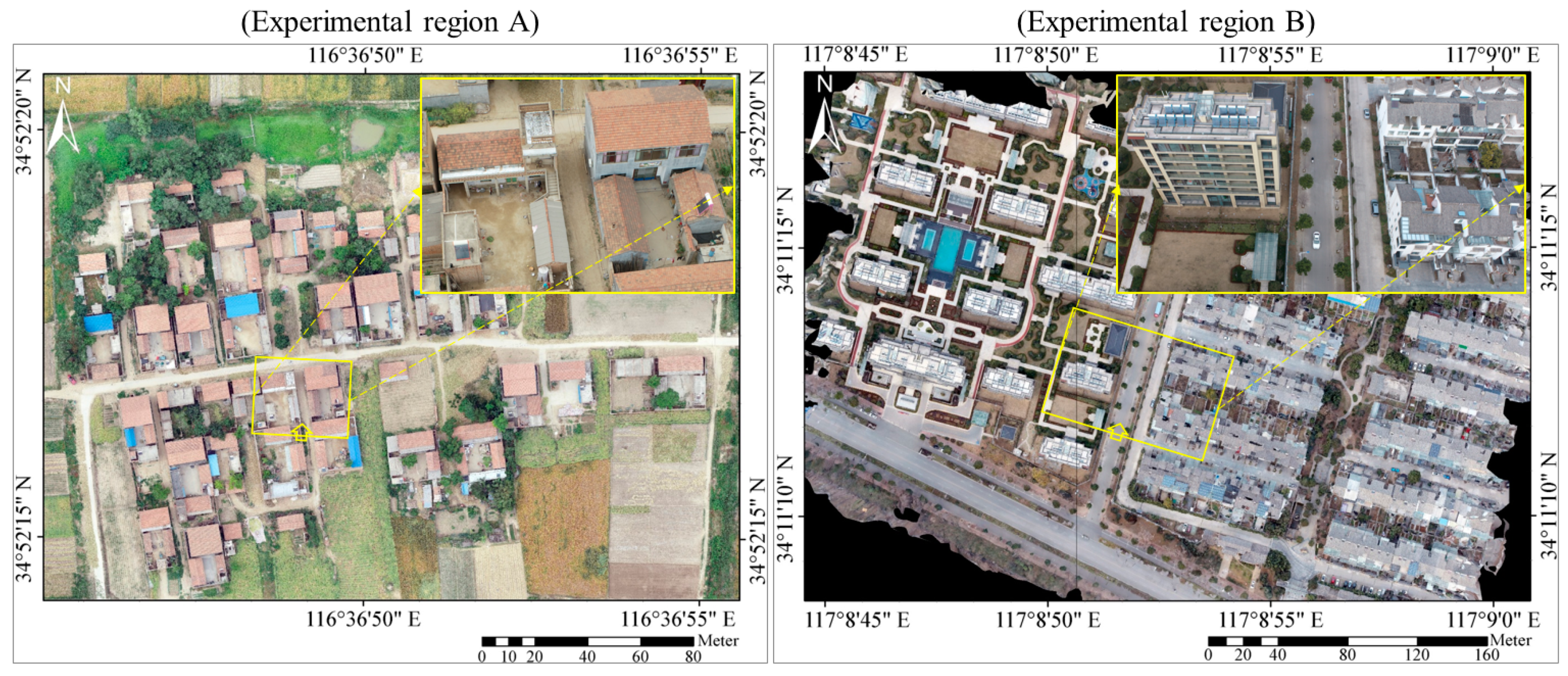
Improving the automation level of building vectorization in the Chinese rural cadastral survey is the original intention of the algorithm implementation in this paper. Therefore, this paper first chooses a countryside as the experimental region to verify the algorithm’s performance. And then, to verify the generalization ability of the algorithm, this paper chooses a city with a broader range of building types as another experimental area. The algorithm’s performance is verified in two experimental areas with different architectural styles. Both experimental regions are in Xuzhou City, China, and the situation and location are shown in Figure 9.
Experimental region A is located in a rural area, with diverse architectural styles and close arrangements, and is easily blocked by trees and other buildings. Experimental region B is located in the inner city. Its west side is a new commercial high-rise residential building with simple features and clear textures and structure. Its east side is an old residential area with complex, close arrangements and disorganized structure. Overall, both experimental regions are representative in China.
3.1.3. The Task Parameters
The flight parameters of the UAVs in the two experimental regions are shown in Table 2.
The experimental images were all collected from five directions (one orthographic and four −60 degree oblique), and 2397 and 585 images were collected from test areas A and B, respectively. The resolutions of the output dense point clouds were 1.80 cm 2.22 cm, respectively.
3.2. Experiment and Analysis
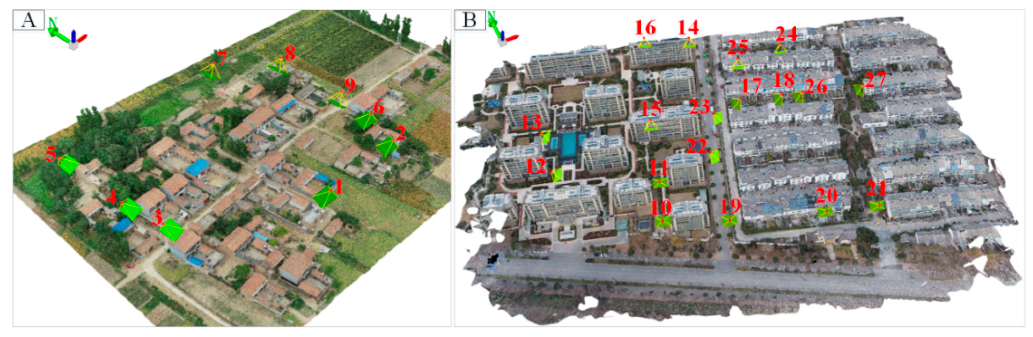
The correctness and accuracy of the detected BEFCP are selected to assess the algorithm’s performance. Twenty-seven images (9 in A; 18 in B), distributed as shown in Figure 10, were selected. The number of correct and incorrect BEFCPs in each image was counted to check the correctness of the algorithm. The coordinates of 23 points (8 in A, 15 in B) with convenient measurement were measured as true values to check the algorithm’s accuracy.
3.2.1. Correctness of the Detected Results
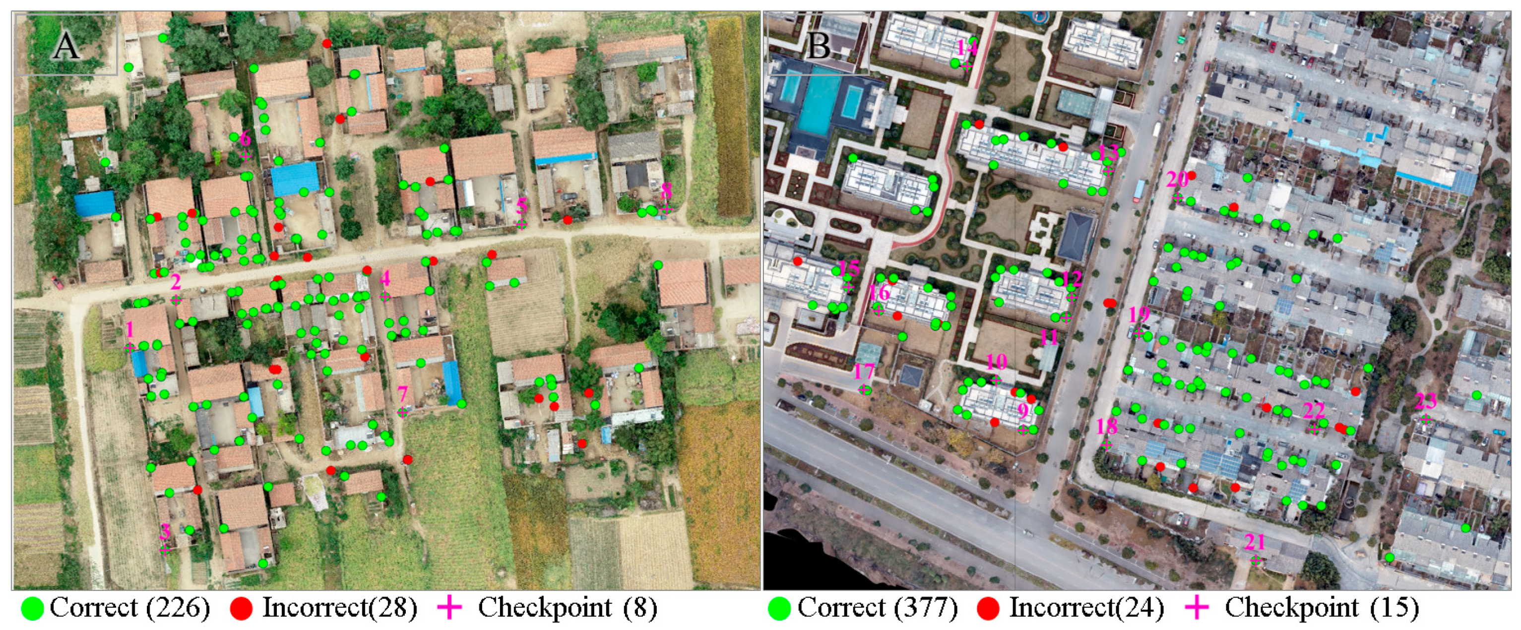
The distributions of experimentally detected BEFCPs are shown in Figure 11.
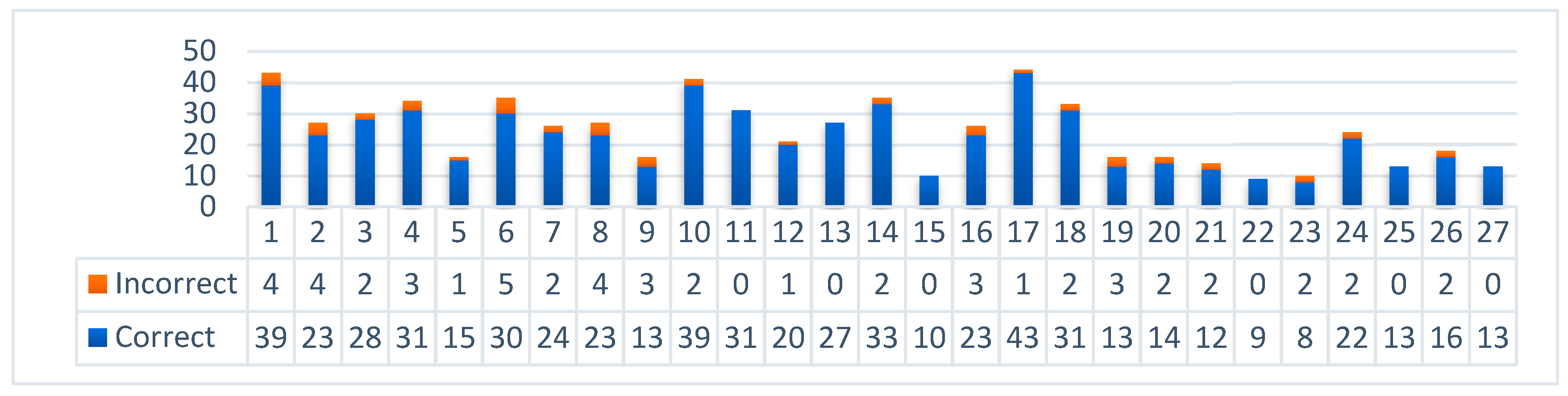
The statistics of detected BEFCPs per image are shown in Figure 12.
The proposed algorithm detected 655 BEFCPs (254 in A, 401 in B) in the experiment (the same building structure may be captured multiple times on different images, so the correct and incorrect BEFCPs may be repetitive), of which 603 (226 in A, 377 in B) were correct, and 52 (28 in A, 24 in B) were incorrect, with a 92.06% (A is 88.98%, B is 94.01%) correct rate. The image with the most BEFCP detected quantity is image 17, with 44 BEFCPs, including 1 incorrect. The image with the lowest BEFCP detected quantity is image 23, with 9 BEFCPs, all correct. The average of BEFCP detected quantity is 24.3 (A is 28.2, B is 22.3). As shown in Figure 11, the 655 BEFCPs from 27 images cover most of the outer contour corner points of the buildings in the target region.
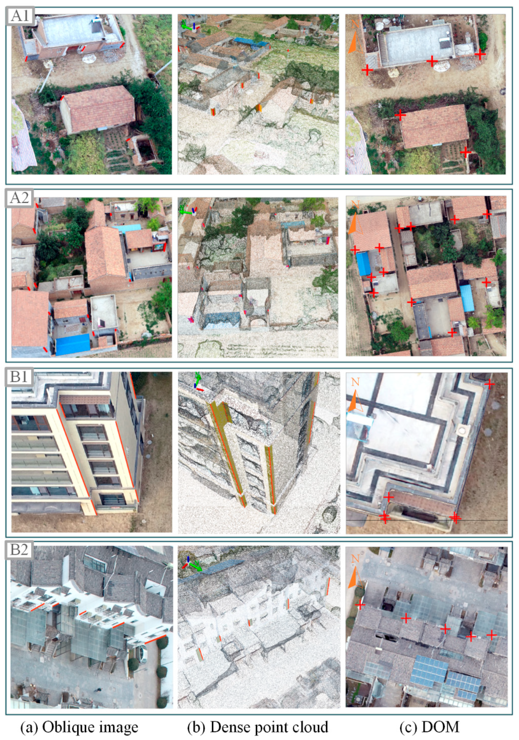
Part of the detected BEFCPs and intermediate process data was transferred to the original oblique image, dense point cloud, and DOM, respectively, to show the partial building contour corner point fitting and extraction results more clearly. As shown in Figure 13, the spatial vertical plane transformed by the 2D fitted straight line fits the structure of the building contour surface well.
3.2.2. Accuracy of the Detected Results
The checkpoints are selected from 23 BEFCPs (index 1 to 8 are in A, index 9 to 23 are in B) near the ground, and their distribution is shown in Figure 11. The coordinates of the building exterior contour corner points corresponding to the BEFCPs are measured from the total station set up at the mapping control points.
The accuracy comparison analysis of the calculation and measurement results of checkpoints is shown in Table 3.
Taking point as an instance, the true errors and of its X and Y coordinates are calculated as and , respectively, and the MSE (mean squared error) of the point position . For the data consisting of points, the overall MSE of point position .
Among the 23 BEFCP checkpoints extracted by the proposed algorithm, the maximum MSE is ±0.072 m, the minimum MSE is ±0.029 m, and the MSE of the overall data is ±0.045 m (A is ±0.042 m, B is ±0.046 m), which can satisfy the high accuracy requirement for the mapping tasks represented by cadastral surveys and large-scale topographic maps.
4. Discussion
This paper combines oblique photogrammetry images and point clouds to achieve high-accuracy and high-precision extraction of BEFCPs. The algorithm can extract some high-quality building exterior facade corner points, effectively improving the production efficiency of building vectors in large-scale topographic mapping, cadastral surveying, and other surveying and mapping production tasks.
Building structures have significant style differences due to geographical, cultural, and other factors, while the basic principle and operating conditions ensure the good generalization of the proposed algorithm. First, the algorithm is based on the commonality of buildings in verticality, which makes it adaptable to the complex textures and structural changes of actual buildings. Second, only part of the plumb line needs to be visible when the algorithm runs, which makes the algorithm effective in densely built areas and areas with partial tree occlusion. Consequently, the basic principle and operating conditions guarantee the algorithm’s good generalization ability.
This paper chooses strict hyperparameters for determining plumb lines in images, point cloud spatial query buffer distance, and spatial plumb line determination to cope with the quality problems of aerotriangulation and the coordinate conversion error problems from image coordinates to world coordinates. First, suppose the overall completion accuracy of the aerotriangulation task is poor. In that case, it will affect the solution results of the camera’s internal and external orientation elements and the accuracy of the dense point cloud generation. In addition, in the perspective imaging model, the camera distortion inversion cannot be directly realized, and an approximate solution is generally obtained by iteration. These all cause errors in the coordinate conversion of the corresponding relationships between homonymous objects in the image and world coordinates. Finally, we prefer the latter regarding the high detection rate and accuracy. The low detection rate can be compensated by the data characteristic of high overlap rate in low-altitude UAV oblique aerial photography. Therefore, we try to maintain the strictness of the parameters. The strict setting of these parameters reduces the detection rate of single-image building exterior outline points. Still, it brings higher accuracy to the algorithm, making it more valuable for application.
This paper initially used two vertical line segments to fit the building facade contour. Still, the actual building corners are close to but not strictly perpendicular to each other. The point cloud obtained from oblique photographic dense matching is thicker and noisier than the radar point cloud, especially in the exterior facade of the building, which also results in a more significant error in the experiments instead, limiting the algorithm’s applicability. Therefore, we finally enlarged the angle tolerance of fitting the wall surface and thus found more diverse and accurate BEFCPs. However, the segmented fitted line as a qualitative condition for building exterior corner points is not robust enough. The lower residual sum of squares represents the more accurate fitting result and the higher accuracy of detection results. Still, the rationality of the two fitting line segments, such as length ratio and direction, should also be considered. Moreover, the segmented linear fit often loses validity when the point cloud is clumped rather than linearly distributed, which is the main reason for the erroneous BEFCP determination. These are the directions for the improvement of the algorithm.
In the experiment, the same plumb line will appear multiple times in different images and participate in the calculation of BEFCPs multiple times. When determining the plumb line from the image, errors in the deviation calculation with the photo nadir point will appear due to different image distortion correction parameters, resulting in false or missed detection. And when restoring the spatial position of the plumb line and extracting the point cloud, some plumb lines may not be able to accurately restore the spatial position due to aerotriangulation accuracy problems and then extract the wrong point cloud, resulting in missed judgment. But, overall, the repeated appearance of plumb lines positively affects the detection of BEFCPs. Taking plumb line P1 and P2 of different images corresponding to the same BEFCP as an example, due to uncertainty problems such as aerotriangulation accuracy, P1 may not be able to restore accurate spatial position, while P2 has higher overall accuracy and successfully extracts the neighboring point cloud, thus being able to extract the BEFCP successfully. The plumb line in the image is the initial estimate of the BEFCP’s position, and the point cloud near the plumb line determines the accuracy of the BEFCP’s positioning. Therefore, their fitting position deviation is minimal when detection is repeated. Integrating repeated detection results can theoretically reduce computational load and further improve the stability of BEFCP position accuracy.
Finally, the algorithm still needs more research to improve the completeness rate of a single building’s BEFCP. The completeness rate of a BEFCP is related to many factors, such as the structure of the building, the distribution of the images, the shooting angle of the images, the accuracy of aerotriangulation, the accuracy of the dense point cloud, etc. The UAV-based DEM (digital elevation model) generated by the point cloud after removing surface points or selecting ground points can accurately represent the topography [28,29,30]. The screening of building point clouds can be achieved by comparison with DEMs, which will directly improve the efficiency of the BEFCP extraction algorithm and is more conducive to achieving the complete extraction of building corner points. This paper mainly verifies the effectiveness of the image combined with point cloud mode for BEFCP extraction. The future research direction is to improve the detection rate of BEFCPs and construct a complete building exterior outline, including DEM-based extraction of a building’s point cloud, the reasonable design of shooting angles, and image selection, building individualization, and regularization.
5. Conclusions
The BEFCP is the positioning basis for buildings in high-precision topographic and cadastral surveys. Currently, the collection of BEFCPs in mapping production tasks relies on manual work, which suffers from heavy tasks and low accuracy, severely limiting production efficiency.
This paper designed a novel BEFCP extraction algorithm combining UAV images and dense point clouds. The proposed algorithm solves the precise positioning problem of point clouds characterizing building structures using the back-calculated plumb line from the UAV images with good accuracy and positioning precision. Moreover, the algorithm is based on the outer walls’ vertical properties and is applicable to all UAV oblique photography-based building vector production tasks, with good generalizability.
The algorithm realizes the extraction of BEFCPs based on the strategy of planar to stereo and rough to precise and consists of four steps: plumb line back-calculation, plumb line spatial mapping, point cloud extraction and filtering, and BEFCP determination and location. The original contributions of this paper in each step are summarized as follows.
- (1)
- Plumb line back-calculation. We designed a plumb line back-calculation algorithm based on vanishing point theory, calculated the photo nadir point from the image, and back-calculated the plumb line in space as the index for building exterior facade corner point retrieval.
- (2)
- Plumb line spatial mapping. We designed an elevation interpolating algorithm of the photographic ray and the dense point clouds to realize the coordinate conversion of the image point to object point, then mapped the line segments in the image to space.
- (3)
- Point cloud extraction and filtering. Based on the characteristics of the high density and high signal-to-noise ratio of the data, we designed a point cloud radius filtering algorithm based on the signal-to-noise ratio to realize the filtering and denoising of the 3D point cloud in the XY 2D space.
- (4)
- BEFCP determination and location. Based on the vertical distribution characteristics of the point cloud near the building exterior facade corner point in the XY 2D plane, a segmented linear least squares fitting algorithm based on the long axis orientation and the farthest point segmentation position constraints was designed to fit the distribution of the building’s structure for the determination and the positioning of the BEFCP.
In the experiment, the algorithm achieved 92.06% correctness, and the overall MSE of the extracted building exterior facade corner points was only ±4.5 cm, which can satisfy the highest accuracy demand of mapping production tasks, e.g., 1:500 topographic maps, property surveys, etc.
The high-quality BEFCPs of the algorithmic outputs can effectively improve the efficiency and automation of building vector manual production, thus possessing high application value. Subsequent research will focus on improving the integrity of BEFCP detection results.
Author Contributions
Conceptualization, X.Z. and J.S.; methodology, X.Z.; software, X.Z.; validation, X.Z., J.S. and J.G.; formal analysis, J.G.; investigation, J.S.; resources, J.S.; data curation, X.Z.; writing—original draft preparation, X.Z.; writing—review and editing, J.S.; visualization, X.Z.; supervision, J.G.; project administration, J.S.; funding acquisition, J.S. All authors have read and agreed to the published version of the manuscript.
Funding
This work was supported by the Second Batch of Jiangsu Province Industry-University-Research Cooperation Projects in 2022 under grant No. BY20221385 and the National Natural Science Foundation of China (NSFC) under grant No. 41171343.
Data Availability Statement
The data that support the findings of this study are available from the corresponding author, J.S., upon reasonable request.
Acknowledgments
The authors would like to acknowledge the Shandong Zhi Hui Di Xin Engineering Technology Co. for providing the UAV and oblique photogrammetry software.
Conflicts of Interest
The authors declare no conflict of interest.
References
- Liasis, G.; Stavrou, S. Building extraction in satellite images using active contours and colour features. Int. J. Remote Sens. 2016, 37, 1127–1153. [Google Scholar] [CrossRef]
- Avudaiammal, R.; Elaveni, P.; Selvan, S.; Rajangam, V. Extraction of buildings in urban area for surface area assessment from satellite imagery based on morphological building index using SVM classifier. J. Indian Soc. Remote Sens. 2020, 48, 1325–1344. [Google Scholar] [CrossRef]
- Zhang, L.; Wang, G.; Sun, W. Automatic extraction of building geometries based on centroid clustering and contour analysis on oblique images taken by unmanned aerial vehicles. Int. J. Geogr. Inf. Sci. 2022, 36, 453–475. [Google Scholar] [CrossRef]
- Maltezos, E.; Doulamis, N.; Doulamis, A.; Ioannidis, C. Deep convolutional neural networks for building extraction from orthoimages and dense image matching point clouds. J. Appl. Remote Sens. 2017, 11, 042620. [Google Scholar] [CrossRef]
- Shi, Y.; Li, Q.; Zhu, X.X. Building segmentation through a gated graph convolutional neural network with deep structured feature embedding. ISPRS J. Photogramm. Remote Sens. 2020, 159, 184–197. [Google Scholar] [CrossRef] [PubMed]
- Li, W.; He, C.; Fang, J.; Zheng, J.; Fu, H.; Yu, L. Semantic segmentation-based building footprint extraction using very high-resolution satellite images and multi-source GIS data. Remote Sens. 2019, 11, 403. [Google Scholar] [CrossRef]
- Pan, X.; Zhang, C.; Xu, J.; Zhao, J. Simplified object-based deep neural network for very high resolution remote sensing image classification. ISPRS J. Photogramm. Remote Sens. 2021, 181, 218–237. [Google Scholar] [CrossRef]
- Harris, C.; Stephens, M. A combined corner and edge detector. Alvey Vis. Conf. 1988, 15, 10–5244. [Google Scholar]
- Smith, S.M.; Brady, J.M. SUSAN—A new approach to low level image processing. Int. J. Comput. Vis. 1997, 23, 45–78. [Google Scholar] [CrossRef]
- Rublee, E.; Rabaud, V.; Konolige, K.; Bradski, G. ORB: An efficient alternative to SIFT or SURF. In Proceedings of the 2011 International Conference on Computer Vision, IEEE, Barcelona, Spain, 6–13 November 2011; pp. 2564–2571. [Google Scholar]
- Remondino, F. Detectors and descriptors for photogrammetric applications. Int. Arch. Photogramm. Remote Sens. Spat. Inf. Sci. 2006, 36, 49–54. [Google Scholar]
- Chen, L.; Rottensteiner, F.; Heipke, C. Feature detection and description for image matching: From hand-crafted design to deep learning. Geo-Spat. Inf. Sci. 2021, 24, 58–74. [Google Scholar] [CrossRef]
- Sharma, S.K.; Jain, K.; Shukla, A.K. A Comparative Analysis of Feature Detectors and Descriptors for Image Stitching. Appl. Sci. 2023, 13, 6015. [Google Scholar] [CrossRef]
- Li, L.; Li, B.; Shen, Y.; Xu, R. UAV Image Detecting of Single Building’s Angular Points Method Based on SVM. Bull. Surv. Mapp. 2017, 78, 52–57. [Google Scholar] [CrossRef]
- Wang, J.; Feng, D.; Chen, J. A building boundary regularization method by contrasting Harris operator and Susan operator. Bull. Surv. Mapp. 2020, 4, 11–15. [Google Scholar] [CrossRef]
- Cui, S.; Yan, Q.; Reinartz, P. Complex building description and extraction based on Hough transformation and cycle detection. Remote Sens. Lett. 2012, 3, 151–159. [Google Scholar] [CrossRef]
- Turker, M.; Koc-San, D. Building extraction from high-resolution optical spaceborne images using the integration of support vector machine (SVM) classification, Hough transformation and perceptual grouping. Int. J. Appl. Earth Obs. Geoinf. 2015, 34, 58–69. [Google Scholar] [CrossRef]
- Partovi, T.; Bahmanyar, R.; Krauß, T.; Reinartz, P. Building outline extraction using a heuristic approach based on generalization of line segments. IEEE J. Sel. Top. Appl. Earth Obs. Remote Sens. 2016, 10, 933–947. [Google Scholar] [CrossRef]
- Xiao, J.; Gerke, M.; Vosselman, G. Automatic detection of buildings with rectangular flat roofs from multi-view oblique imagery. Int. Arch. Photogramm. Remote Sens. Spat. Inf. Sci. 2010, 38, 251–256. [Google Scholar]
- Xiao, J.; Gerke, M.; Vosselman, G. Building extraction from oblique airborne imagery based on robust facade detection. ISPRS J. Photogramm. Remote Sens. 2012, 68, 56–68. [Google Scholar] [CrossRef]
- Zhuo, X.; Fraundorfer, F.; Kurz, F.; Reinartz, P. Optimization of OpenStreetMap building footprints based on semantic information of oblique UAV images. Remote Sens. 2018, 10, 624. [Google Scholar] [CrossRef]
- Nex, F.; Rupnik, E.; Remondino, F. Building footprints extraction from oblique imagery. ISPRS Ann. Photogramm. Remote Sens. Spat. Inf. Sci. 2013, 2, 61–66. [Google Scholar] [CrossRef]
- Acar, H.; Karsli, F.; Ozturk, M.; Dihkan, M. Automatic detection of building roofs from point clouds produced by the dense image matching technique. Int. J. Remote Sens. 2019, 40, 138–155. [Google Scholar] [CrossRef]
- Zhang, J.; Li, L.; Lu, Q.; Jiang, W. Contour clustering analysis for building reconstruction from LiDAR data. In Proceedings of the International Archives of the Photogrammetry, Remote Sensing and Spatial Information Sciences, Beijing, China, 3–11 July 2008; Volume 37, pp. 355–360. [Google Scholar]
- Song, J.; Wu, J.; Jiang, Y. Extraction and reconstruction of curved surface buildings by contour clustering using airborne LiDAR data. Optik 2015, 126, 513–521. [Google Scholar] [CrossRef]
- Wu, B.; Yu, B.; Wu, Q.; Yao, S.; Zhao, F.; Mao, W.; Wu, J. A graph-based approach for 3D building model reconstruction from airborne LiDAR point clouds. Remote Sens. 2017, 9, 92. [Google Scholar] [CrossRef]
- Von Gioi, R.G.; Jakubowicz, J.; Morel, J.-M.; Randall, G. LSD: A fast line segment detector with a false detection control. IEEE Trans. Pattern Anal. Mach. Intell. 2008, 32, 722–732. [Google Scholar] [CrossRef]
- Alper, A. Evaluation of accuracy of dems obtained from uav-point clouds for different topographical areas. Int. J. Eng. Geosci. 2017, 2, 110–117. [Google Scholar]
- Yilmaz, V.; Konakoglu, B.; Serifoglu, C.; Gungor, O.; Gökalp, E. Image classification-based ground filtering of point clouds extracted from UAV-based aerial photos. Geocarto Int. 2018, 33, 310–320. [Google Scholar] [CrossRef]
- Fan, J.; Dai, W.; Wang, B.; Li, J.; Yao, J.; Chen, K. UAV-Based Terrain Modeling in Low-Vegetation Areas: A Framework Based on Multiscale Elevation Variation Coefficients. Remote Sens. 2023, 15, 3569. [Google Scholar] [CrossRef]
Figure 1.
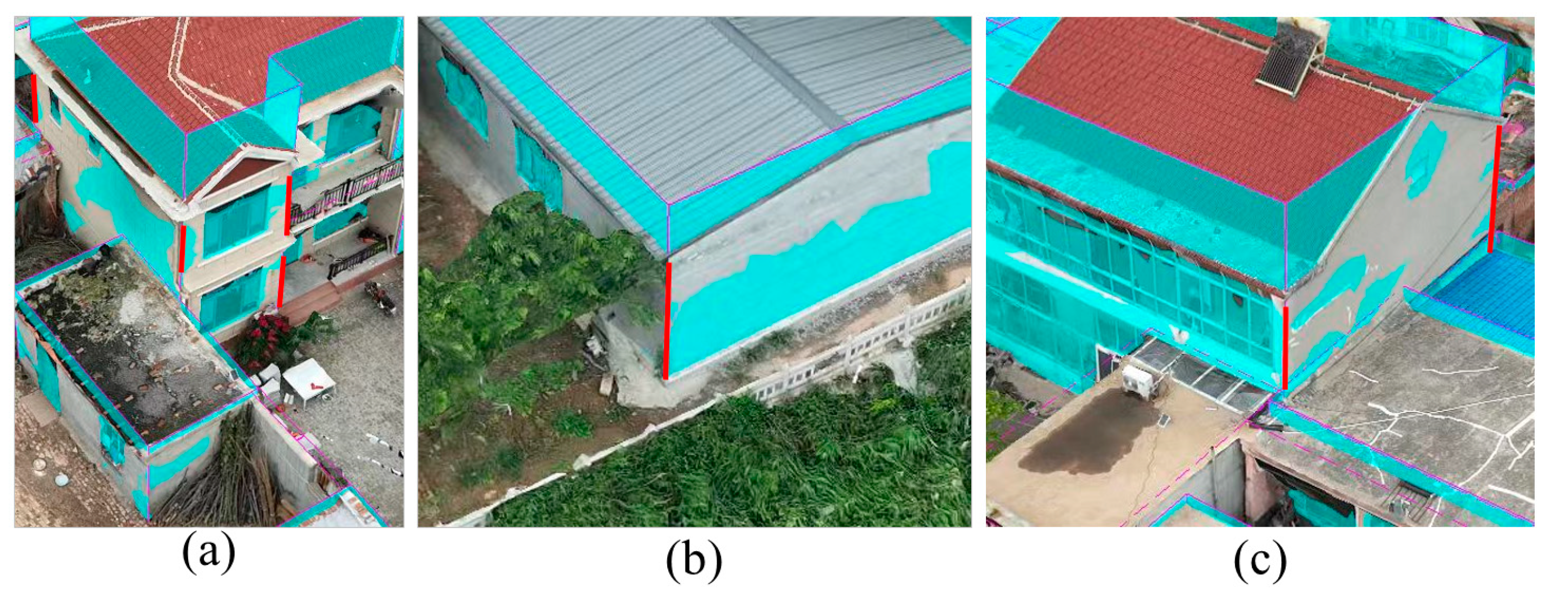
Examples of BEFCPs. The red lines are the corner lines of the exterior facade of the building, and the corresponding points of the corner lines in the XY plane are BEFCPs. A BEFCP is not the corner point of the building footprint. It is usually located on the plumb line of the building facade under the roof and is the basis for accurately measuring the area of land occupied by a building. In large-scale topographic mapping, cadastral surveying, and other surveying and mapping production tasks in China, the primary production method for BEFCPs is for indoor workers to operate the real-scene 3D mapping software, determine the wall plane using three or five points, and then determine the BEFCP using the intersection line of the wall planes. The buildings have complex structures and are close to each other (as shown in (c)), and BECFP is occluded by eaves and trees (as shown in (a,b)). Accurately retrieving the point cloud representing BEFCP (point cloud in the neighborhood with the red line) and recovering the building structure from discrete point clouds are the key to locating BEFCPs.
Figure 1.
Examples of BEFCPs. The red lines are the corner lines of the exterior facade of the building, and the corresponding points of the corner lines in the XY plane are BEFCPs. A BEFCP is not the corner point of the building footprint. It is usually located on the plumb line of the building facade under the roof and is the basis for accurately measuring the area of land occupied by a building. In large-scale topographic mapping, cadastral surveying, and other surveying and mapping production tasks in China, the primary production method for BEFCPs is for indoor workers to operate the real-scene 3D mapping software, determine the wall plane using three or five points, and then determine the BEFCP using the intersection line of the wall planes. The buildings have complex structures and are close to each other (as shown in (c)), and BECFP is occluded by eaves and trees (as shown in (a,b)). Accurately retrieving the point cloud representing BEFCP (point cloud in the neighborhood with the red line) and recovering the building structure from discrete point clouds are the key to locating BEFCPs.

Figure 2.
Examples of plumb line extensions intersecting at the photo nadir point. Aerial imaging belongs to the central projection, where the projections of parallel lines in the world coordinate system on the image intersect at the vanishing point. Plumb lines are a unique set of parallel lines in the real world, and their extensions intersect at the photo nadir point in the image space.

Figure 3.
The flow of BEFCP recognition algorithm.

Figure 4.
Schematic diagram of line segment extraction: (a) is a screenshot of the details of straight lines extracted directly from the original image using the LSD, while (b) performs BF before extracting the straight lines. The red circles are areas of significant contrast where the BF enhances most of the edges of the building structure and effectively blurs the building interior and tree textures.

Figure 5.
Examples of back-calculation and spatial mapping of plumb lines. Figures (lb) and (rb) are enlargements of the red boxes in figures (la) and (ra), respectively. Images preserve tight texture features clearly distinguishing spatially adjacent building structure feature lines, providing accurate spatial indices for extracting point clouds characterizing building structures after the plumb lines are mapped to space.

Figure 6.
Algorithm flow of coordinate calculation of object point corresponding to the image point, where “a” is the image point, “A” is the object point corresponding to “a”, and “S” is the photo-graphic ray connecting “A” and “a”.
Figure 6.
Algorithm flow of coordinate calculation of object point corresponding to the image point, where “a” is the image point, “A” is the object point corresponding to “a”, and “S” is the photo-graphic ray connecting “A” and “a”.

Figure 7.
Examples of the point cloud extraction, filtering, and fitting process. After dimensionality reduction, the original point clouds show stronger spatial aggregation, and the point cloud filtering algorithm eliminates its noise.
Figure 7.
Examples of the point cloud extraction, filtering, and fitting process. After dimensionality reduction, the original point clouds show stronger spatial aggregation, and the point cloud filtering algorithm eliminates its noise.

Figure 8.
BEFCP determination and positioning algorithm flow.

Figure 9.
Situation and location maps of the experimental regions.

Figure 10.
Experimental image distribution maps. The distribution of 27 experimental images in test areas (A,B). The red numbers are the image index numbers, the red dot is the photography center, and the yellow line and green quadrilateral are the shooting poses.
Figure 10.
Experimental image distribution maps. The distribution of 27 experimental images in test areas (A,B). The red numbers are the image index numbers, the red dot is the photography center, and the yellow line and green quadrilateral are the shooting poses.

Figure 11.
Distributions of BEFCP detection results and checkpoints. The green and red circles are the correctly and incorrectly detected BEFCPs, respectively, and the red crosses are the selected positional accuracy checkpoints.
Figure 11.
Distributions of BEFCP detection results and checkpoints. The green and red circles are the correctly and incorrectly detected BEFCPs, respectively, and the red crosses are the selected positional accuracy checkpoints.

Figure 12.
Statistical chart of the detected amount of BEFCPs.

Figure 13.
Examples of correct detection results. The red line and the red “+” are the BEFCP’s mapping results in the image, the point cloud, and the DOM, respectively. The top and bottom exterior facade corner points in a high-rise building with extreme spatial proximity are correctly distinguished and identified, as shown in (B1). The corner points under the roof are also accurately fitted and identified, as shown in (A1,B2). The BEFCP is still successfully detected when the composition of the exterior facade of the building is complex, and the plumb line where the BEFCP was located was only partially extracted, as shown in (A2).


Table 1.
Main parameters of DJI PHANTOM 4 RTK.
| Aircraft | |||
| Type | Four-axis aircraft | Hovering accuracy | ±0.1 m |
| Horizontal flight speed | ≤50 km/h (Positioning mode) | Single flight time | Approx. 30 min |
| Camera | |||
| Image sensor | 1-inch CMOS; 20 million effective pixels (20.48 million total pixels) | Camera Lens | FOV 84°; 8.8 mm/24 mm; Aperture f/2.8–f/11; with autofocus |
| Maximum photo resolution | 5472 × 3648 (3:2) | Photo format | JPEG |
| Platform | |||
| Controlled rotation range | Pitch: −90° to +30° | Stabilization system | 3-axis (pitch, roll, yaw) |
| Maximum control speed | Pitch: 90°/s | Angular jitter | ±0.02° |
| GNSS (Global Navigation Satellite System) | |||
| GNSS | GPS + BeiDou + Galileo (Asia region); GPS + GLONASS + Galileo (other regions) | RTK GNSS | Positioning accuracy: Vertical 1.5 cm + 1 ppm (RMS); Horizontal 1 cm + 1 ppm (RMS) |
Table 2.
UAV flight task parameters.
| Parameter | Experimental Region A | Experimental Region B |
|---|---|---|
| Flight height | 55 m | 80 m |
| Flight speed | 3.9 m/s | 6.3 m/s |
| Camera photography angle | −60 degrees | −60 degrees |
| Lateral overlap rate | 70% | 70% |
| Forward overlap rate | 80% | 80% |
Table 3.
Checkpoint plane error table (Unit: meters).
| Index | Calculation Coordinate | Measurement Coordinate | Point True Error | Point MSE | |||
|---|---|---|---|---|---|---|---|
| 1 | 464,607.7895 | 3,860,373.551 | 464,607.8069 | 3,860,373.579 | 0.017 | 0.028 | 0.033 |
| 2 | 464,620.2741 | 3,860,386.442 | 464,620.298 | 3,860,386.391 | 0.024 | −0.051 | 0.056 |
| 3 | 464,617.2427 | 3,860,318.763 | 464,617.2594 | 3,860,318.737 | 0.017 | −0.026 | 0.031 |
| 4 | 464,676.9509 | 3,860,387.38 | 464,676.9842 | 3,860,387.356 | 0.033 | −0.024 | 0.041 |
| 5 | 464,713.9601 | 3,860,407.023 | 464,713.9161 | 3,860,407.039 | −0.044 | 0.016 | 0.047 |
| 6 | 464,639.1039 | 3,860,425.45 | 464,639.143 | 3,860,425.425 | 0.039 | −0.025 | 0.046 |
| 7 | 464,681.6341 | 3,860,356.08 | 464,681.6085 | 3,860,356.111 | −0.026 | 0.031 | 0.040 |
| 8 | 464,753.2681 | 3,860,411.214 | 464,753.2409 | 3,860,411.177 | −0.027 | −0.036 | 0.045 |
| 9 | 513,590.6049 | 3,784,342.831 | 513,590.5763 | 3,784,342.852 | −0.029 | 0.021 | 0.035 |
| 10 | 513,580.4271 | 3,784,361.856 | 513,580.3666 | 3,784,361.88 | −0.060 | 0.024 | 0.065 |
| 11 | 513,606.8909 | 3,784,385.762 | 513,606.8298 | 3,784,385.788 | −0.061 | 0.026 | 0.067 |
| 12 | 513,608.9105 | 3,784,393.517 | 513,608.9405 | 3,784,393.503 | 0.030 | −0.014 | 0.033 |
| 13 | 513,622.7851 | 3,784,441.72 | 513,622.7967 | 3,784,441.684 | 0.012 | −0.036 | 0.037 |
| 14 | 513,569.3097 | 3,784,481.885 | 513,569.3274 | 3,784,481.907 | 0.018 | 0.022 | 0.029 |
| 15 | 513,524.4945 | 3,784,397.56 | 513,524.4482 | 3,784,397.588 | −0.046 | 0.028 | 0.054 |
| 16 | 513,535.9423 | 3,784,388.363 | 513,535.8774 | 3,784,388.332 | −0.065 | −0.031 | 0.072 |
| 17 | 513,530.2823 | 3,784,358.265 | 513,530.2995 | 3,784,358.231 | 0.017 | −0.033 | 0.037 |
| 18 | 513,622.1615 | 3,784,337.167 | 513,622.1134 | 3,784,337.147 | −0.048 | −0.021 | 0.052 |
| 19 | 513,634.3369 | 3,784,379.841 | 513,634.2978 | 3,784,379.875 | −0.039 | 0.035 | 0.052 |
| 20 | 513,649.1241 | 3,784,431.598 | 513,649.1015 | 3,784,431.641 | −0.023 | 0.043 | 0.049 |
| 21 | 513,678.6969 | 3,784,293.087 | 513,678.6717 | 3,784,293.104 | −0.025 | 0.017 | 0.030 |
| 22 | 513,700.8003 | 3,784,343.198 | 513,700.816 | 3,784,343.239 | 0.016 | 0.041 | 0.044 |
| 23 | 513,743.0917 | 3,784,346.914 | 513,743.1304 | 3,784,346.926 | 0.039 | 0.011 | 0.040 |
Disclaimer/Publisher’s Note: The statements, opinions and data contained in all publications are solely those of the individual author(s) and contributor(s) and not of MDPI and/or the editor(s). MDPI and/or the editor(s) disclaim responsibility for any injury to people or property resulting from any ideas, methods, instructions or products referred to in the content. |
© 2023 by the authors. Licensee MDPI, Basel, Switzerland. This article is an open access article distributed under the terms and conditions of the Creative Commons Attribution (CC BY) license (https://creativecommons.org/licenses/by/4.0/).
Share and Cite
MDPI and ACS Style
Zhang, X.; Sun, J.; Gao, J. An Algorithm for Building Exterior Facade Corner Point Extraction Based on UAV Images and Point Clouds. Remote Sens. 2023, 15, 4166. https://doi.org/10.3390/rs15174166
AMA Style
Zhang X, Sun J, Gao J. An Algorithm for Building Exterior Facade Corner Point Extraction Based on UAV Images and Point Clouds. Remote Sensing. 2023; 15(17):4166. https://doi.org/10.3390/rs15174166
Chicago/Turabian StyleZhang, Xinnai, Jiuyun Sun, and Jingxiang Gao. 2023. "An Algorithm for Building Exterior Facade Corner Point Extraction Based on UAV Images and Point Clouds" Remote Sensing 15, no. 17: 4166. https://doi.org/10.3390/rs15174166
Note that from the first issue of 2016, this journal uses article numbers instead of page numbers. See further details here.