
Tempo-Spatial Landslide Susceptibility Assessment from the Perspective of Human Engineering Activity

1
College of River and Ocean Engineering, Chongqing Jiaotong Univeristy, Chongqing 400047, China
2
Faculty of Engineering, China University of Geosciences, Wuhan 430074, China
3
ENGAGE—Geomorphic Systems and Risk Research, Department of Geography and Regional Research, University of Vienna, 1010 Vienna, Austria
4
School of Civil and Transportation Engineering, Hebei University of Technology, Tianjin 300401, China
5
School of Earth Sciences, China University of Geosciences, Wuhan 430074, China
*
Author to whom correspondence should be addressed.
†
These authors contributed equally to this work.
Remote Sens. 2023, 15(16), 4111; https://doi.org/10.3390/rs15164111
Submission received: 13 July 2023
/
Revised: 17 August 2023
/
Accepted: 18 August 2023
/
Published: 21 August 2023
/
Corrected: 29 November 2023
(This article belongs to the Special Issue Landslide Inventory Mapping and Monitoring Using Remote Sensing Techniques)
Abstract
:The expansion of mountainous urban areas and road networks can influence the terrain, vegetation, and material characteristics, thereby altering the susceptibility of landslides. Understanding the relationship between human engineering activities and landslide occurrence is of great significance for both landslide prevention and land resource management. In this study, an analysis was conducted on the landslide caused by Typhoon Megi in 2016. A representative mountainous area along the eastern coast of China—characterized by urban development, deforestation, and severe road expansion—was used to analyze the spatial distribution of landslides. For this purpose, high-precision Planet optical remote sensing images were used to obtain the landslide inventory related to the Typhoon Megi event. The main innovative features are as follows: (i) the newly developed patch generating land-use simulation (PLUS) model simulated and analyzed the driving factors of land-use land-cover (LULC) from 2010 to 2060; (ii) the innovative stacking strategy combined three strong ensemble models—Random Forest (RF), Extreme Gradient Boosting (XGBoost), and Light Gradient Boosting Machine (LightGBM)—to calculate the distribution of landslide susceptibility; and (iii) distance from road and LULC maps were used as short-term and long-term dynamic factors to examine the impact of human engineering activities on landslide susceptibility. The results show that the maximum expansion area of built-up land from 2010 to 2020 was 13.433 km2, mainly expanding forest land and cropland land, with areas of 8.28 km2 and 5.99 km2, respectively. The predicted LULC map for 2060 shows a growth of 45.88 km2 in the built-up land, mainly distributed around government residences in areas with relatively flat terrain and frequent socio-economic activities. The factor contribution shows that distance from road has a higher impact than LULC. The Stacking RF-XGB-LGBM model obtained the optimal AUC value of 0.915 in the landslide susceptibility analysis in 2016. Furthermore, future road network and urban expansion have intensified the probability of landslides occurring in urban areas in 2015. To our knowledge, this is the first application of the PLUS and Stacking RF-XGB-LGBM models in landslide susceptibility analysis in international literature. The research results can serve as a foundation for developing land management guidelines to reduce the risk of landslide failures.
1. Introduction
Global climate change increases the frequency and severity of typhoon events [1]. In recent years, catastrophic typhoons have occurred frequently in coastal areas around the world, resulting in numerous geological disasters [2,3,4,5]. The southeastern coast of China, which is bordered by the Pacific Ocean, is susceptible to landslides caused by typhoons. Every year, there are a large number of casualties and economic losses [6,7,8]. To date, the Chinese government has attempted to prevent landslide disasters by establishing a geological hazard warning system that includes weather forecasting [9,10,11,12]. However, the annual economic losses are still increasing. A large part of this is due to the continuous transformation of the geological environment by human engineering activities [13,14]. In the past few years, China’s urbanization index has rapidly increased from 0.157 in 2000 to 0.438 in 2015 [15]. In areas with strong engineering activities, the Typhoon-triggered rainstorm was more likely to cause landslide disasters. Therefore, we urgently need to explore the characteristics of changes in human engineering activities on the occurrence of landslides.
Land-use and land-cover are often used to describe the impact of human engineering activities, including natural elements (water bodies, forests, cropland, and grassland) and human-modified surfaces (building activity areas). Many researchers found that LULC may alter the distribution of landslide susceptibility caused by rainfall [16,17,18]. For instance, Pisano et al. [19] analyzed the hill and low mountain areas of the Italian Southern Apennines land-use change and concluded that increasing forest and cropland area can reduce the susceptibility to landslides. Rohan et al. [20] focused on the Southern Pennsylvania area and analyzed that urbanized areas are usually more prone to landslides, which are closely related to distance from roads and terrain curvature. Hao et al. [21] analyzed the LULC dataset in Kerala, India, from 2000 to 2018 and found that landslides mainly occur in forest areas. In China, human activities and urban expansion have become the main causes of landslides in recent decades, accounting for approximately 70% of the total number [22]. Chen et al. [23] compiled two types of LULC maps with a time interval of 21 years (1992–2013) and analyzed that even if cropland and grassland were converted to forestland, the susceptibility of landslides still increased. Xiong et al. [22] analyzed the changes in landslide susceptibility in Enshi City using landslide inventories from 2000 and 2020 and changes in LULC maps. Given that human activities can rapidly change vast areas, the LULC map may require more predictive scenarios. Promper et al. [24] used the Dyna-CLUE model to analyze LULC changes in Austria over 138 years (1962–2100) to simulate the evolution of landslide risk. Tyagi et al. [18] proposed the ANN-CA model to predict the LULC in 2030 and analyzed the variation patterns of landslides. Guo et al. [25] utilized the land change modeler (LCM) integrated into IDRISI Selva software to obtain LULC maps for 2040 and 2080 and analyzed the susceptibility of shallow landslides in Wanzhou, China. Shu et al. [26] also used the LCM software to explore how LULC in the Varan region of Spain has changed with landslide susceptibility over the past 150 years (1946–2097). Past prediction models had limited capabilities in investigating the causes of land-use changes. Moreover, using dynamic simulations to evaluate patch-level alterations of various land-use types over time and space was challenging [27,28]. In 2021, the High performance Spatial Computational Intelligence Lab of China University of Geosciences (Wuhan) developed the patch generating land-use simulation (PLUS) model to explore the driving factors of multiple types of land expansion and predict patch-level evolution of LULC [28]. This model has made outstanding progress in the study of land-use analysis in China [27,29,30,31]. This article is the first attempt to explore the impact of LULC change on landslides using the PLUS model. In addition, a point often overlooked in many studies is to consider road distance as a static factor without considering its dynamic characteristics [18,19]. Generally speaking, road construction directly affects slopes through changes in road cut or surface water runoff. Therefore, this study explores the effects of road network and LULC changes on landslide susceptibility.
Currently, most of the literature evaluates the spatial probability (or susceptibility) of landslides by focusing on environmental and geographical factors [32,33,34,35,36]. The production of landslide susceptibility maps with accurate, up-to-date, and reliable information is the focal point. With the rapid development of artificial intelligence and computer science, machine learning models have been widely used for landslide susceptibility assessment. More specifically, the shift from traditional statistical models to data-driven models fundamentally directly affects the predictive performance of susceptibility modeling [37]. The widely used machine learning models currently include decision trees (DT) [38,39,40], multi-layer perceptron network (MLPNN) [41,42], support vector machine (SVM) [43,44,45], etc. Furthermore, some scholars have attempted to use ensemble models to enhance and improve the prediction errors of single classifiers. The Random Forest model is the earliest and most widely used ensemble model. The prediction accuracy of landslide susceptibility has been greatly improved by the integration of the bagging algorithm and decision tree model [46,47]. Similarly, based on gradient enhancement methods (i.e., gradient boosting decision tree (GBDT), XGBoost, and LightGBM), the model with predicted errors is strengthened and improved by the principle of reusing residual patterns [48,49]. Dou et al. [50] integrated the basic model SVM using bagging, boosting, and stacking algorithms to explore the susceptibility distribution of shallow landslides in Japan. However, the limitations of these models are evident, i.e., optimal performance varies across different research areas. For example, He et al. [48] analyzed the susceptibility of landslides and wildfires in Southeast Asia and obtained that the prediction accuracy of Random Forest model is always higher than GBDT and Adaptive Boosting model. Wang et al. [51] found that the RF model (area under the receiver operating characteristic (ROC) curve, AUC = 0.88) outperformed XGBoost (AUC = 0.86) in the study area of Wuqi County in the hinterland of the Loess Plateau. Liu et al. [52] found that the GBDT model is better than the RF model in spatial modeling of shallow landslides near Kvam, Norway. Due to variations in model operation strategies and sensitivity to datasets, it is challenging to identify a model with strong generalization capabilities that consistently performs optimally across diverse research areas [34]. Therefore, some scholars have attempted the hybrid strategy of strong classifiers. Li et al. [53] adopted a stacking strategy to integrate the convolutional neural network (CNN) and recurrent neural network (RNN), and the results showed that the proposed framework could retain the best predictive capability (AUC = 0.918) compared to CNN (AUC = 0.904) and RNN (AUC = 0.900). Arabameri et al. [54] compared the modeling AUC values of credal decision tree (CDT), Alternative Decision Tree (ADTree), and their ensemble method (CDT-ADTree) of 0.837, 0.867, and 0.981, respectively. In the analysis of landslide susceptibility in the Three Gorges Reservoir area, Zeng et al. [34] compared and analyzed various ensemble strategies (bagging, boosting, and stacking) and basic models (DT, SVM, MLPNN, XGBoost, and RF). They found that the stacking strategy, which ensembles strong models like XGBoost and RF, yielded optimal prediction accuracy and generalization ability. Therefore, appropriate ensemble strategies can help researchers obtain models with stronger robustness. In particular, more and more attention has been paid to the application of the hybrid model to landslide susceptibility analysis. We should explore the impact of the hybrid model and dynamic human engineering activities on landslide occurrence.
The southeast coastal mountainous areas of China are affected by typhoon-triggered rainstorms all year round. Land-use change (such as deforestation, agricultural, and urban regional expansion) and road network expansion have aggravated the occurrence of landslide disasters. In this study, we used high-precision optical remote sensing images to obtain the landslide inventory triggered by Typhoon “Megi” in 2016. The main purpose of this study is to explore the relationship between LULC and road network on the susceptibility of landslides triggered by typhoons. The innovations include the following: (i) We adopted the newly developed PLUS model to simulate various factors, and utilized historical LULC imagery to forecast the LULC long-term dynamic factors for both 2030 and 2060; concurrently, the road network distribution from 2018 to 2020 was harnessed as a short-term dynamic factor. (ii) In a novel approach, we combined the RF, XGBoost, and LightGBM models through a stacking strategy to delineate the susceptibility relationship between influential factors and landslides. (iii) Furthermore, we assessed the susceptibility distribution of typhoon-induced landslides under diverse human engineering activity scenarios. To our knowledge, this marks the pioneering application of both the PLUS and the stacked RF-XGB-LGBM models in landslide susceptibility research.
2. Study Area
2.1. Geography and Geological Conditions
The research area, situated in the middle of the circum Pacific coastline of the Chinese Mainland (Figure 1a), in the southeast of Zhejiang Province, near the East China Sea (Figure 1b). The landform is trapezoidal from northwest to southeast, which can be divided into the middle- and low-mountains in the northwest, the low-mountains, hills, and basins in the middle, and the mudflat area in the eastern plain. Covering 2067.55 km2, it reaches a peak elevation of 1150 m (Figure 1c). Geologically, this region is positioned in the north section of the Mesozoic volcanic rock belt in the southwest of the Pacific continental margin volcanic rock belt. Quaternary sediments in mountainous areas are mainly distributed in small and medium-sized valleys and local mountainous areas. The accumulation is mainly alluvial and proluvial, with a thickness of 5–10 m. The sediments in plain areas are mostly transitional from terrestrial to marine. The area rests on the southeastern edge of the Eurasian Plate and is affected by the collision of the Pacific Plate. The low mountain landforms in the study area are mostly composed of sandstones, volcanistic rocks, glutenite, and carbonate rocks (Figure 1d). The rock structure fractures are not developed, with a high degree of weathering and a layer thickness of 5–6 m, making it susceptible to geological disasters. According to the monitoring of the China Geological Survey, the seismic activity in the study area is not strong, with low occurrence probability. Climatically, the area enjoys a subtropical monsoon climate, averaging 18 °C with an annual rainfall exceeding 1700 mm. The region experiences the “plum rain” season from May to June, resulting from the confluence of warm, humid airflows from the south and cooler, dry ones from the north. Typhoons, frequent between July and September, coupled with high rainfall, pose significant geological disaster risks. Over the past 20 years, escalating human engineering activities, particularly road construction, have compromised slope stability, with over 90% of landslides triggered by typhoon-induced rainstorms.
2.2. Description and Analysis of Landslide Inventory
In 2016, the 17th Typhoon “Megi” landed in Zhejiang Province of China on 27 September and ceased operations on 29 September. The Typhoon caused a heavy rainstorm. According to the disaster management system of the China Meteorological Administration and the China Geological Environment Monitoring Institute, the rainfall events triggered by the Typhoon caused many landslides, resulting in 32 deaths and three missing people. It also caused serious damage to infrastructure, such as buildings, transmission line towers, and roads. A detailed and accurate landslide inventory is an important foundation for landslide susceptibility assessment. With the advancement of sensors and space technology, remote sensing can obtain detailed temporal and spatial information about landslides on the Earth’s surface. After the Typhoon event, we immediately carried out a comprehensive landslide mapping activity. This study used two high-resolution optical satellite images of Planet (3 m resolution) to evaluate the failure boundary (https://www.planet.com/, 18 November 2019). The satellite data were obtained before and after the event, namely in August 2016 and November 2016, respectively. These images cover the entire study area and have low cloud cover (Figure 2). Zhang et al. [55], Geertsema et al. [56], and Saito et al. [57] described the importance of high-quality Planet satellites in drawing landslide inventories. All landslides are related to this single rainfall event, thus representing an event-based inventory. Field investigations have shown that most of the landslides in the study area belong to planer slides [58]. It has been observed that some of the slides have evolved into mountain slope mudslides, with relatively long propagation distances and even affecting some gentle slopes. Finally, we established a landslide inventory for Typhoon “Megi” event, which includes 1124 landslides. Among them, 748 areas are larger than 1000 m2. The average area is 2088.49 m2, and the maximum area is 33,391.21 m2, and the minimum area is 916.52 m2.
3. Materials and Methods
Figure 3 provides an overview of the steps involved in this study’s application. The landslide inventory is derived from the visual interpretation of two time-separated high-precision optical remote sensing images. The basic data for modeling landslide susceptibility includes seven static factors (slope, aspect, plane curve, profile curve, hydrology, DEM, and soil type) and two dynamic factors (LULC and distance from road). Based on data availability, distance from road was only considered as a short-term dynamic factor considering changes from 2016 to 2020. The PLUS model was used to predict LULC maps from the past to the future for the years 2030 and 2060. This step is based on the obtained conditioning factors, and LULC maps from 2010 and 2020. The hybrid model was applied to landslide susceptibility modeling, with the following primary innovative characteristics: (i) the use of Bayesian optimization to obtain the optimal parameters for the RF, XGBoost, and LightGBM models, and (ii) the application of a stacking strategy to combine these three optimized strong ensemble models. Finally, we investigated the distribution of landslide susceptibility under different engineering scenarios.
3.1. Data Collection and Processing
3.1.1. Land-Use Land-Cover Conditioning Factors
This study mainly considered land-use land-cover, socio-economic, and climate-environmental data. The LULC datasets were provided by the Data Center for Resources and Environmental Sciences, Chinese Academy of Sciences (RESDC) (http://www.resdc.cn, 20 November 2022). The LULC data in 2010 mainly used Landsat TM/ETM remote sensing images, and the LULC data in 2015 and 2020 mainly used Landsat 8 remote sensing images. The datasets were reclassified into six categories: cropland, forestland, grassland, water area, and built-up land, with the 30 × 30 m spatial resolution. The research area shows a relatively small area of unused land, and Google Image cross-validation shows that the translated unused land is actually built-up land. Therefore, this article categorizes unused land into built-up land for analysis.
Socio-economic and climatic environmental data were selected as potential drivers of urban expansion (Table 1). GDP, population, annual average temperature, and annual average precipitation were obtained from the 1 km spatial resolution grid data provided by the RESDC (https://www.resdc.cn/, 20 November 2022). The distribution data of oil type is the vectorized 30 m resolution data from Nanjing Institute of Soil, Chinese Academy of Sciences. An open-source platform, OpenStreetMap (https://www.openstreetmap.org/, 20 November 2022), is used to obtain vector data of road network and water systems. In the ArcGIS platform, the distance from road and river was measured in the Euclidean distance tool. All factors were resampled to the pixel data with a spatial resolution of 30 m. DEM data was extracted based on ASF Data Search data (https://search.asf.alaska.edu, 20 November 2022).
3.1.2. Influencing Factors Used as Landslide Predictors
The influencing factors are necessary information for statistical correlation with the presence and absence of observed landslides, used to construct a susceptibility map [46,59,60,61]. Reichenbach et al. [37] and Lima et al. [62] reviewed the most commonly used geological and terrain prediction factors for landslide susceptibility modeling in machine learning assessments. Some of these factors remained essentially unchanged during the analysis time range. For example, geological factors can be considered time-invariant. Similarly, terrain features also exhibit a slow rate of time variation and can be approximated as time-invariant. On the contrary, LULC has been proven to be dynamic over long-time spans (decades) [63]. At the same time, the short-term change factor that many studies overlook—road network—is a very clear dynamic signal in China, where infrastructure is rapidly developing. In this study, the factors influencing landslides were selected based on both data availability for the study area and literature reviews [20,26,50]: (i) static factors, digital elevation models (DEM), and geology and (ii) dynamic factors and human engineering activities. In the ArcGIS platform, secondary terrain factors such as slope, aspect, plane curvature, and profile curvature were generated from the DEM. All spatial factors were resampled to a resolution of 30 m. An overview of the spatial distribution of these factors and their internal categories in the study area is shown in Figure 4. The lithology in geological factors shows the main distribution of sandstones (SS), volcanic rocks (VR), and glutinite (Glut) in the study area. Planar sliding is common in sandstone, especially when the inclination direction is consistent with the dip of the rock layer [64,65]. Glutenite and volcaniclastic rock are mainly located on steep slopes in mountainous areas, usually completely to strongly weathered. The soil type is mainly classified as laterite soil (LS), followed by yellow soil (YS), paddle soil (PS), and brown forest soil (BFS). Table 1 shows the sources of the LULC dataset, and we used the data from 2015 to model landslide susceptibility. The OpenStreetMap obtained the road network distribution from 2016 to 2020. The road network of the research area was analyzed by merging in 2017 and 2018, as there were no significant differences. The Euclidean distance in the ArcGIS platform was used to calculate the distance from road. The results show a gradual decrease in road distance.
3.2. Data Collection and Processing
The patch generating land-use simulation model was developed by the High performance Spatial Computational Intelligence Lab of China University of Geosciences (Wuhan) in 2021 [28,66]. The model proposes a new land expansion analysis strategy (LEAS), which can avoid exponential growth of transformation types with categories. Specifically, the RF model was used to analyze the driving relationship between the expansion of LULC and the conditioning factors in two periods, so as to obtain the development probability of each land-use type and the weight of each conditioning factor. The interpretability of the model provides a mechanism for exploring LULC change and simulating the generation and evolution of multiple random LULC patches [29]. In addition, PLUS model provides a new model based on multiple random seeds cellular automata (CARS), which automatically generates dynamic simulation patches under development probability constraints, and drives the total LULC based on local micro land-use changes [27]. Finally, its operating speed is much superior. Therefore, the PLUS model was used to better evaluate the evolution process and predict future changes in the distribution of LULC. The operation processes of PLUS model are as follows:
(1) We extracted the LULC expansion from 2010 to 2020 based on the land expansion module in PLUS software. Then, eleven conditioning factors were used to generate the development probability and factor contribution for each type of LULC.
(2) Based on LULC data from 2010 and 2020, the Markov Chain predicted the demand for LULC types in 2030. The CARS module combines land development probability, land demands, transition matrix, and neighborhood weights to obtain the predicted LULC distribution map. The transition matrix considered the socio-economic development and natural environmental characteristics of the study area, limiting the conversion of water systems into other land-use patterns (Table 2). The neighborhood weights are calculated based on the proportion of expanded area for each LULC type:
where Xi is the neighborhood weight of type i; ΔTAi is the change in land-use type i; ΔTAmax and ΔTAmin represents the maximum and minimum values of land-use expansion area, respectively.
(3) We closed 2010 as the baseline starting time and used the development probability of each LULC from 2010 to 2020 to predict the data in 2020. The validation module in PLUS software was used to input actual and predicted LULC data for 2020. The model validation was usually carried out through Kappa coefficients [30,67]. Kappa coefficients calculate the overall accuracy (OA) classification through confusion or accuracy matrices. The accuracy matrix returns the accuracy of producers, which is a measure of consistency between observed data and modeled data. Usually, Kappa coefficients greater than 0.8, and can be considered as a perfect simulation result [67]. Ultimately, our goal is to simulate LULC map for 2030 and 2026.
3.3. Hybrid Model for Landslide Susceptibility Assessment
The ensemble model selects the basic classifier with relatively weak classification performance, and finally obtains a strong classifier through the ensemble strategy. The most effective ensemble strategy currently is bagging and boosting algorithm. The former trains multiple “weak and different” classifiers through sample diversity and feature diversity, and then integrates the output results through voting or mean methods; the latter continuously optimizes the learning strategy by increasing the importance and weight of misclassified samples through concatenation, ultimately gradually improving the final output.
Random Forest is a typical bagging model created by Breiman [68]. This model randomly samples different subsets from the data to establish multiple different decision trees and integrates the results of a single decision tree according to bagging’s rules (regression means average, classification means minority follows majority). The samples at the root node of the decision tree are randomly selected from the training set to extract N bootstrap samples. Each node of the decision tree randomly selects m of these M attributes for splitting (m << M). The structure of a single decision tree will increase the overall complexity and overfitting degree of RF model.
XGBoost is a new generation boosting model based on the comprehensive upgrade of GBDT model [69]. The XGBoost model mainly uses boosting algorithm for modeling. The Loss function L(x, y) adaptively influences the construction of the next weak classifier f(x)k according to the result f(x)k−1 of the previous classifier. The running goal of the GBDT model is to find the minimum value of the Loss function L(x, y) and minimize the difference between the predicted and real results. This process only cares about accuracy, not complexity or overfitting. The XGBoost model adds the structural risk term of controlling overfitting to the Loss function. This strategy makes the XGBoost different from other boosting models as the model is trained towards the goal of minimizing the objective function, rather than minimizing the Loss function. XGBoost model prioritizes the use of parameters in structural risk to control the overfitting, rather than relying on the decision tree structure parameters (such as the maximum depth of the tree, learning rate, etc.). This step improves the prediction accuracy and generalization ability of XGBoost, and also enables the model’s wide use in data competitions and industrial production.
LightGBM is a model derived from the XGBoost and applied to industrial practice [70]. The XGBoost model requires the preservation of data feature values and ranking, resulting in significant space consumption. LightGBM has introduced the Histogram algorithm to optimize the traditional XGBoost model, which can accelerate the training velocity without compromising accuracy. Histogram algorithm discretizes the continuous floating-point eigenvalues into K integers, and constructs a histogram with the width of K. After traversing the data, the histogram accumulates the required statistics, and traverses to find the optimal segmentation point. The histogram optimization algorithm proposed by LightGBM can handle compressed data very well, ultimately significantly improving the training efficiency of each tree.
However, although the ensemble model already has many optimization strategies, practical applications still need to test different types of models to obtain better results. The ‘strong yet different’ RF, XGBoost, and LightGBM models can be very suitable for future model integration to achieve a better model. The widely used stacking strategy can better combine multiple strong classifiers to obtain better results [34,71]. Unlike voting and averaging methods, the stacking strategy achieves model combination by training a secondary classifier (rather than finding a weighted average). In this process, the original individual classifiers are considered to as the first-level classifier, while the model used in the combination process is referred to as the second-level classifier. The stacking algorithm obtains the advantages of multiple strong classifiers to establish a new hybrid model, which improves prediction accuracy. The specific process is as follows:
(i) The research area adopted a raster format with a pixel size of 30 m. The unit point turning function in GIS environment was used to obtain attribute data of all influencing factors within the region. The GIS database includes all units within the study area, with attribute values for nine influencing factors. In the Python environment, 8173 landslide units (value = 1) and 8173 non-landslide units (value = 0) were divided into two parts: 70% of the units were randomly selected as the training dataset, and the remaining 30% were used as the testing dataset.
(ii) In our study, we chose Bayesian optimization for hyperparameter tuning due to its known efficiency in high-dimensional spaces, especially beneficial for complex models like XGboost and lightGBM. Its data-efficient nature, which is paramount when model evaluations are computationally intensive as with 10-fold cross-validation, and its unique sequential strategy, where hyperparameters are evaluated in succession based on insights from previous evaluations, made it particularly suitable. Given the limited 1000 evaluations and the depth of our hyperparameter search space detailed in Table 3, Bayesian optimization was an optimal choice. The meaning of optimization parameters is as follows: N_estimators, the number of basic estimators; Max_depth, the maximum depth of basic estimators; Min_sample_split, the minimum number of split samples; Min_samples_leaf, the minimum number of leaf samples; Lr, the learning rate; Subsample, the proportion of used samples; Colsample_bytree, the proportion of random sampling each tree; Colsample_bylevel, the proportion of random sampling features at each level; Colsample_bynode, the proportion of random sampling each leaf node; Num_leaves, the number of leaf nodes in a tree; Min_split_gain, the minimum weight sum of split nodes; and Min_child_samples, the minimum number of leaf samples.
(iii) It is worth noting that in order to prevent information leakage, optimization and hybrid strategies were carried out on the training dataset, with a 30% testing dataset used for the final model performance evaluation. Three optimized ensemble models were applied to the first-level classifier. The logistic regression model was used as a stacking secondary classifier. Finally, we obtained the hybrid model stacking RF-XGB-LGBM.
4. Results
4.1. Analysis of Temporal and Spatial Variation Characteristics of LULC
The area size LULC types in the research area are forestland > cropland > grassland > built-up land > water area (Table 4). From 2010 to 2020, grassland, built-up land, and water increased by 0.139, 13.443, and 0.037 km2, respectively; the cropland and forestland decreased by 6.031 and 7.589 km2.
From 2010 to 2020, the area transfer reached 57.477 km2 (Table 5). The transferred-out land in the study area mainly comes from forestland and cropland, with the transferred-out areas of 28.23 and 20.727 km2 and 49.12% and 36.06% of the total transferred out area, respectively; the transferred in land is mainly forestland, cropland and built-up land, which are 35.92%, 25.56%, and 25.33%, respectively. The expansion area of the water body did not change, mainly due to most of the water in the study area being controlled by hydropower stations, maintaining a relatively stable water area. The expansion area of grassland is only 0.139 km2. The maximum expansion area of built-up land is 13.433 km2, mainly expanding forestland and cropland, with 8.28 km2 and 5.99 km2, respectively. According to equation (1), we calculated the neighborhood weights for different LULC types. It is worth mentioning that the calculation results of grassland, water, and built-up land are 1, 0.008, and 0, respectively. To avoid the absoluteness of probability, we have corrected these three weights to 0.9, 0.1, and 0.1.
We entered LULC maps for 2010 and 2020 and extracted the expanded area for each type. The LEAS module obtains the development probability of each LULC type and the contribution of different conditioning factors to expansion. Furthermore, we analyzed the factor contributions and main factors of cropland, forestland, and built-up land (Figure 5). The main driving factors for the expansion of cropland are distance from third-level roads, distance from government, annual rainfall, and distance from rivers. Cropland activities were dominated by human engineering activities and required sufficient water resources for irrigation. The increase in cropland was mainly distributed in areas closer to third-level roads (Figure 5a). Figure 5b shows that the distance from second-level road has the greatest impact on forestland expansion, followed by slope, distance from third-level road, and DEM. Most of the areas with increased forestland were mainly concentrated in the area far from the road, with higher slopes and elevations. DEM has the greatest impact on the expansion of built-up land area, followed by distance from government (Figure 5c). The increase in built-up land is mainly distributed around government residences in areas with relatively flat terrain and frequent socio-economic activities.
The accuracy of the PLUS model determines the authenticity of the experimental results. We incorporate the 2010 LULC map into the PLUS model to simulate the 2020 LULC map and compare it with the actual LULC map in 2020. The results show that the Kappa coefficient is 0.904, and the overall accuracy is 0.965, indicating that the model can effectively simulate the dynamic changes of LULC in the study area. Furthermore, based on the actual 2020 LULC map, we used the CARS module to simulate the land-use changes in 2030 and 2060 (Figure 6). Final simulation of 2030 LULC map contains 269.78 km2 cropland, 1614.89 km2 forestland, 104.93 km2 grassland, 29.70 km2 water, and 48.25 km2 built-up area; 2060 LULC map contains 257.07 km2 cropland, 1593.77 km2 forestland, 105.23 km2 grassland, 29.95 km2 water, and 81.54 km2 built-up area.
4.2. Factor Performance
The primary analysis objective of landslide influencing factors must be to confirm whether the factor set is highly correlated. Highly correlated factors can bring redundant information and interfere with the predictive function of the model. The multicollinearity analysis of Pearson correlation coefficients was used to test this function [72]. Figure 7a shows a weak correlation with |r| values < 0.5. Therefore, we determined that all factors are relatively independent and used for subsequent analysis. The operational logic and random feature selection of ensemble models result in differences in attention to input features. As shown in Figure 7, the RF model tends to use aspect (0.209), distance from road (0.182), and DEM (0.149); the XGBoost model focuses more on soil (0.180), LULC (0.163), lithology (0.161), and distance from road (0.141); LightGBM generated higher scores for distance from road (3945), DEM (3447), and aspect (2892). The strong and independent ensemble model provides a better guarantee for the results of the model hybrid strategy. However, it should be noted that land-use has a very low contribution in both the RF model and the LightGBM model. The active landslide is closely related to the distance from the road, especially in areas close to roads, the number of landslides is highest (Figure 7e). The land-use shows that the forestland area has the highest number of landslides, followed by cropland and grassland (Figure 7f).
4.3. Assessing Modeling Patterns
Before using cross-validation to evaluate modeling accuracy, we would like to remind readers of an important aspect that is often overlooked in the literature. When using spatially dependent data, we must have robust non-parametric methods to validate, select, and evaluate the predictive accuracy of the model. Ideally, model validation, selection, and prediction errors should be calculated using independent data. Therefore, we used the training set for 10-fold cross-validation here and used the test set to evaluate the final prediction ability. The cross-validation strategy for parameter optimization is also carried out on the training set. This methodology can test the overfitting ability of the model. The model optimization parameters are shown in Table 6. As shown in Figure 8, it starts from the independent evaluation of the cut-off point of the report summary of the receiver operating characteristic (ROC) obtained through each of the 10 iterations. The optimal performance model for 10-fold cross-validation was LightGBM (mean AUC = 0.9), followed by XGBoost (mean AUC = 0.898), and finally RF (mean AUC = 0.889). The Stacking strategy has improved prediction accuracy, with an average AUC of 0.908. The following Figure 9 corresponds to the calibration plot and the average prediction probability distribution of the model. The calibration plot is obtained from the average prediction probability and the fraction of positive classes in each bin. Perfectly calibrated to fit diagonally in the graph (prediction probability equals empirical probability). The performance of the Stacking model is very stable, and the prediction probability is close to the diagonal. The average prediction probability shows that the RF model exhibits a certain degree of uncertainty in the prediction of the entire dataset. The XGBoost and LightGBM models have similar predicted distributions and exhibit extreme predictions. The Stacking model integrates bagging and boosting algorithms, reducing overall uncertainty. This is also reflected in the error rate, which is stable at around 0.19. These are important considerations that support our model not only as an explanatory tool but also as a robust predictive tool.
We used test set data to evaluate the predictive ability of the model in fields that have never appeared before. In general, discrimination categories are regarded as No discrimination (AUC = 0.5), Acceptable (0.8 ≤ AUC < 0.9), Excellent (0.8 ≤ AUC < 0.9), and Outstanding (0.9 ≤ AUC) [73]. Figure 10 provides an overview, with an RF model prediction accuracy of 0.887, which is basically consistent with the training set; the AUC values of XGBoost and LightGBM models are 0.893 and 0.898, respectively. The Stacking model achieved an excellent AUC value of 0.915. The final result shows an improvement in the generalization ability of the hybrid model. After demonstrating the predictive ability of our spatiotemporal susceptibility model, in this section, we transform the model results into maps. The susceptibility map needs to further process steps where the continuous spectrum of probability values is divided into multiple categories. Based on the fixed level division, the reconstructed susceptibility maps were subdivided into very low (0 ≤ S < 0.05), low (0.05 ≤ S < 0.35), moderate (0.35 ≤ S < 0.75), and high (0.75 ≤ S ≤ 1.00) levels [34]. According to observations, there are significant differences in the appearance of susceptibility maps (Figure 11). Generally speaking, the RF model generates low spatial contrast prediction patterns in the region, resulting in a considerable number of pixels in the lower and flatter parts of the catchment area, resulting in lower susceptibility scores. XGBoost and LightGBM have good predictive performance for known landslide areas but lack exploration of other areas. The visual interpretation of the Stacking RF-XGB-LGBM model indicates a general consistency between the corresponding landslide inventory location and areas classified as moderate or highly susceptible. The hybrid model clearly reproduced the observed higher and lower landslide distribution patterns in the figure and was considered the ultimate application tool. The next section will specifically discuss using simulation methods to generate future scenarios.
4.4. Prediction Patterns over Different Engineering Scenarios
We examined various engineering scenarios to develop comprehensive prediction patterns. The scenarios considered include:(i) All static factors remained constant, with the exception of two parameters associated with human engineering activity. (ii) For short-term predictions, the road networks from 2018, 2019, and 2020 were considered. Land-use and land-cover data from 2015 was maintained constant across these scenarios, which are labeled as RL1–RL3. (iii) Long-term forecasting involves two main scenarios. In the combined change (RLP1 & RLP2) scenarios, we take into account alterations in the road network data from 2020, paired with predictions in LULC changes. Meanwhile, in the Land-use changes only (LP1 & LP2) scenarios, our focus is solely on the predicted LULC variations, keeping the road data from 2016 unchanged. (iv) We defined areas within a 200 m radius of further urbanization as directly affected areas.
All the engineering scenarios are detailed and outlined in Table 7. This program may be interesting as it conveys the direct impact of disasters on local and future communities. It is worth noting that the 2017 road network is the same as the 2018 road network; therefore, we did not consider the operating scenarios of the 2017 road network.
The landslide susceptibility maps for 2018, 2019, and 2020 were predicted using the Stacking RF-XGB-LGBM model and road network changes as dynamic factors. Changes in the susceptibility region can be observed in Figure 12. Significant changes in susceptibility levels were observed in the southwest and northwest of the study area from 2016 to 2018. Among them, the susceptibility level of very-low decreased by 17.18%, and the susceptibility level of low, model, and high increased by 6.2%, 15.94%, and 7.04%, respectively. From 2018 to 2019, the susceptibility expansion area of the study area mainly occurred in the northwest. The susceptibility of very-low levels decreased by 6.82, and low, moderate, and high levels increased by 3.42%, 1.75%, and 0.45%, respectively. The eastern region experienced expansion from 2019 to 2020. The susceptibility level of very-low and low decreased by 1.33% and 0.05%, respectively; the susceptibility level of moderate and high increased by 1.39% and 1.05%, respectively. Table 8 shows the landslide susceptibility level in urban areas. With the construction of the road network, areas with low, moderate, and high susceptibility areas are gradually increasing. From 2016 to 2020, the very-low susceptibility decreased by 11.96%, and the low, medium, and high susceptibility increased by 11.15%, 26.88%, and 17.72%, respectively. The road networks expansion has greatly increased the probability of landslides occurring in urban areas.
To explore the impact of LULC and road network on susceptibility estimation, we generated landslide susceptibility maps for the study area in 2030 and 2060. Figure 13 compares the urbanization part of the map from two aspects: spatial pattern and susceptibility. Road construction has changed the distribution of susceptibility in the research area; and susceptibility models based on LULC and road networks have generated smoother susceptibility patterns and relatively higher susceptibility in urbanized areas. Furthermore, the susceptibility to landslides increases with the expansion of urbanization areas. These four landslide susceptibility maps highlight slightly different areas that may require further attention. Regardless of the year considered, most of the accumulation zone that are most threatened by landslides are located in the southeast of the study area.
As shown in Figure 14, the statistical analysis of susceptibility values reveals the differences between susceptibility maps modeled based on different operating scenarios. The comparison shows that for the entire study area, only considering changes in LULC (LP1 and LP2), low susceptibility increases, while moderate and high susceptibility decreases slightly. However, it is unrealistic to only consider LULC change, as the development of urban areas was accompanied by road network construction. The landslide susceptibility considering road network factors (RLP1 and RLP2) showed significant percentage changes: a decrease of 9.05% for very-low level, an increase of 5.29% for low level, a moderate increase of 2.96%, and an increase of 0.79% for high susceptibility level. We also observed the impact of scenarios on urbanization areas. The urbanization areas in 2015 showed that human engineering have increased potential risks to a certain extent, such as the percentage of low susceptibility areas increasing from 33.22% to 38.67%; the moderate susceptibility increased from 7.04% to 9.38%; the high susceptibility increased from 5.22% to 6.56%. The predicted urbanization areas in 2030 showed more significant changes in susceptibility level: low susceptibility increased by 12.6%, moderate susceptibility increased by 3.16%, and high susceptibility increased by 0.64%. The 2060 urbanization areas have 31.06% very low, 50.96% low, 11.87% moderate, and 6.12% high susceptibility percentage levels. The RL-U, RLP1-U, and RLP2-U scenarios show that, in 2015 in urbanized areas, the number of pixels with high susceptibility was 1134, 1386, and 1425, respectively. It is obvious that the expansion of road network and LULC will increase the probability of landslide disasters in old urban areas. This comparison helps to quantify whether urbanized areas are more susceptible to landslides before urbanization.
5. Discussion
The current research focus involves considering human engineering activity scenarios and evaluating how they alter landslide susceptibility [63]. Now, ample evidence suggests that landslide susceptibility is dynamic, particularly in the context of rapid urban and road network expansion—a prevalent issue in many developing countries, including China. Especially in the eastern coastal areas of China, policy adjustments have driven a large number of engineering activities [74,75]. Firstly, it is necessary to consider the influence of LULC changes on landslides of mountain area. Accurately predicting future LULC scenarios is crucial for improving susceptibility reliability. Therefore, this study used the PLUS model for the first time in landslide research. This model has high simulation and prediction accuracy for larger regions and can better predict the evolution of future land-use patterns [28,67]. Many studies [27,29,30,76] have confirmed that the PLUS model can simulate LULC changes at different scales and scenarios, providing guidance for sustainable urban development. Eleven conditioning parameters were used to predict the 2060 LULC map: the forestland and cropland areas decreased by 28.53 km2 and 18.07 km2, respectively, and the built-up area increased by 45.88 km2. The land-use in this area is mainly transformed from forests to built-up areas. The increase in built-up land is mainly distributed around government residences with relatively flat terrain and frequent socio-economic activities. Numerous studies have assessed the impact of LULC changes on landslide susceptibility [18,20,22,25]. However, human activities are carried out by road network [77]. The extended road network may lead to rapid changes in urban land-use. Generally, roads enter the susceptibility model based on their distance from the plotted landslide [18,21]. But few researchers have explored the influence of road network changes on landslides. Roads may introduce deviations in the distribution of landslide susceptibility [20]. Therefore, this article has updated the list of road networks and LULC. It should be noted that many researchers have explored the application of different landslide inventory in land-use change, such as Xiong et al. [22] used LULC and landslide inventories from 2000 and 2020 and Tyagi et al. [18] used 218, 243, and 387 landslide events from 2005 to 2010, 2010 to 2015, and 2015 to 2020, respectively. On the contrary, Hao et al. [21] only used the 2018 landslide inventory for dynamic research. The update landslide inventory inevitably has a higher density and quantity of landslides, making it difficult to explore the impact of LULC on susceptibility alone. Therefore, this study focused solely on the landslides triggered by the 2016 Typhoon event to explore the impact of LULC and road network changes on landslide susceptibility, employing nonlinear relationships constructed by hybrid models.
People are more and more interested in the study of the application of hybrid model in landslide susceptibility analysis, especially the effect of human engineering activities on landslide occurrence [63]. In the realm of landslide susceptibility analysis, the integration of models offers a potent approach to enhance prediction capabilities. Our choice of employing a hybrid model, specifically combining RF, XGBoost, and LightGBM, was motivated by several factors. Firstly, each of these models has shown superior predictive prowess individually in previous landslide susceptibility studies [49,78]. While they are adept on their own, their combination allows us to harness their unique strengths and offset individual weaknesses, offering a more robust and comprehensive modeling approach. Secondly, the stacking strategy offers a layer of meta-learning where predictions from individual models are used as input to train a higher-level model, thereby refining predictions. However, no papers attempted to integration and application. The Stacking strategy has started to be applied to integrate basic models. For instance, Li et al. [53] adopted a stacking strategy combined with the convolutional neural network and recurrent neural network to explore the distribution of landslide susceptibility in the Three Gorges Reservoir area. Zeng et al. [34] compared and analyzed the application of different ensemble models and strategies in landslide susceptibility, and found that stacking strategy combined with strong classifiers can maximize the efficiency of improving prediction accuracy. We can find the differences from the factor contribution of ensemble models: the RF model tended to use aspect, distance from road and DEM. The XGBoost model focused more on soil, LULC, hydrology, and distance from road. The LightGBM model generated higher scores for distance from road, DEM, and aspect. A major difference between this study and previous studies is that both RF and LightGBM have low rankings for LULC. This may reflect differences in environmental and/or climatic conditions and LULC categories between this study and previous studies. The results show that distance from road is highly correlated with landslides occurrence. Finally, the stacking RF-XGB-LGBM model achieved the optimal AUC value of 0.915 on the test set. The hybrid model in this study area can be proved to improve the prediction accuracy and generalization ability of landslide susceptibility. We also encourage researchers to attempt the use of more hybrid model. These studies are good attempts to map the susceptibility of landslides in dynamic environments.
The hybrid model explores the road network and LUCL expansion on landslide susceptibility. The density of landslides gradually decreases with the increase in road distance (Figure 7e). This correlation reflects the richness of roads along the valleys in the study area, and nearby slopes are prone to slide. For the whole research area, the regional susceptibility of road network expansion has changed from 2016 to 2020. In 2018, the moderate and high susceptibility areas increased by 15.94% and 7.04%, respectively. Early large-scale engineering construction increased the probability of landslides. Urban areas have been more affected: from 2016 to 2020, the very low susceptibility decreased by 11.96%, while the low, moderate, and high susceptibility increased by 11.15%, 26.88%, and 17.72%, respectively. Most of the landslides that happened in 2016 occurred in forest areas. This is contrary to many other findings in which forest areas were considered to have a stabilizing ability [24,79,80]. However, Lan et al. [81] found that the weight of trees may increase the sliding force in parallel directions. The vegetation structure with different root systems can increase or reduce the susceptibility of shallow landslides [82]. Especially bamboo forests and shrubs are mostly distributed in the research area. The extreme rainfall event in 2016 is more prone to causing a large number of planer slides in forest areas.
We further explored the changes in susceptibility using the predicted LULC maps for 2030 and 2060. For the whole study area, the susceptibility of road networks and LULC to landslides showed significant percentage changes: a decrease of 9.05% for very-low levels, an increase of 5.29% for low levels, a moderate increase of 2.96%, and an increase of 0.79% for high susceptibility. For the urbanized areas in 2015, the expansion of road network and LULC increased the number of landslides with high susceptibility. The urbanization areas in 2030 and 2060 show that LULC has a positive impact on landslides. This may be due to our data lamination of 2020 road network. It is difficult for us to obtain data on future road planning. Therefore, we can conclude that for our research area, road expansion is the main dynamic factor, followed by LULC. The influence of LULC changes on the stability conditions of our study area is positive, but relatively limited. About this point, controversial findings have been reported in the literature. In high mountain areas, the improvement in stability conditions may be significant [83], while other researchers have found that specific changes in LULC (such as deforestation) may also lead to an increase in regional landslide susceptibility [80]. However, there is no doubt that land-use changes in urban areas have brought about unstable factors. The current policy of China will continue to lead to a large number of road network and urban regional expansion in many years. We suggest that the government can provide more road network planning to more precisely describe the landslide area. Through policy interpretation, landslide managers can obtain future land information, such as potential landslide risks in future roads and land built-up areas.
Although this study systematically quantifies the long-term impact of urbanization on landslide occurrence, it is still limited by the dataset and methods used. Our finding used a limited inventory induced by extreme rainfall events. A larger inventory of multi-temporal landslides and more detailed information on the occurrence of landslides at different stages of urbanization may help to better quantify the impact of urbanization on susceptibility. This article does not consider the impact of climate and other environmental factors on the stability conditions of future slopes, especially the prediction of Typhoon induced rainfall events. As future work, we plan to include more aspects in the prediction of human engineering activities. In addition, applying current programs in other regions to test the impact of environmental changes will reveal better insights into this topic.
6. Conclusions
This study explores the individual and joint effects of road network and LULC changes on the stability of Typhoon-triggered landslides in the mountainous areas along the southeastern coast of China. The hybrid model simulates the regional landslide susceptibility of seven engineering scenarios. Finally, we compared the results obtained in each scenario with the reference scenario.
From 2010 to 2020, the rapid urbanization of the research area led to a maximum built-up area of 13.433 km2, mainly expanding forestland and cropland, with 8.28 km2 and 5.99 km2, respectively. The novelty PLUS model was used to predict changes in LULC, and the results indicate an increase in built-up land in the future. The increase in built-up land is mainly distributed around government residences in areas with relatively flat terrain and frequent socio-economic activities. The predicted 2060 LULC map shows that forestland and cropland will decrease by 28.53 km2 and 18.07 km2, respectively, while the built-up area will increase by 45.88 km2.
The hybrid model has improved the prediction accuracy and generalization ability of landslide susceptibility. In the training set, the optimal performance model shown in the 10-fold cross-validation was Stacking RF-XGB-LGBM model (mean AUC = 0.908), followed by LightGBM model (mean AUC = 0.9) and XGBoost model (mean AUC = 0.898), and finally RF model (mean AUC = 0.889). The final testing set showed that the Stacking model achieved an excellent AUC value of 0.915.
The prediction model shows that the factor contribution of distance from road was greater than that of LULC. From 2016 to 2020, the prediction results show that the distance from road has decreased by 11.96% from 2016 to 2020, and the low, medium, and high susceptibility have increased by 11.15%, 26.88%, and 17.72%, respectively.
Ultimately, changes in LULC and road network may disrupt the stability of mountainous areas, endanger natural resources, and damage the environment. These results require more rational land-use and road planning in future urbanization processes, and suggest incorporating LULC changes more systematically in disaster assessment to implement preventive measures from the beginning. This adopted method is novel for landslide susceptibility research in this region.
Author Contributions
Methodology, B.J. and T.Z.; investigation, Z.G.; writing—original draft preparation, T.Z.; writing—review and editing, Z.G. and L.W.; visualization, F.W. and R.G.; funding acquisition, Z.G. All authors have read and agreed to the published version of the manuscript.
Funding
This research is funded by Natural Science Foundation of Hebei Province (D2022202005), National Natural Science Foundation of China (U22A20600), National Key Research and Development Program of China (2021YFB2600604, 2021YFB2600600), National Natural Science Foundation of China (42307248) and National Natural Science Foundation Joint Fund Project (U2034203).
Data Availability Statement
Restrictions apply to the availability of these data. The landslide inventory data and Figure 2 were obtained from Chong Xu, Chenchen Xie, and Yuandong Huang of the National Institute of Natural Hazards, Ministry of Emergency Management of China and their availability requires further permission from Chong Xu ([email protected]).
Conflicts of Interest
The authors declare no conflict of interest.
References
- Ma, S.; Shao, X.; Xu, C. Characterizing the Distribution Pattern and a Physically Based Susceptibility Assessment of Shallow Landslides Triggered by the 2019 Heavy Rainfall Event in Longchuan County, Guangdong Province, China. Remote Sens. 2022, 14, 4257. [Google Scholar] [CrossRef]
- Guo, Z.; Tian, B.; Li, G.; Huang, D.; Zeng, T.; He, J. Danqing Song. Landslide susceptibility mapping in the Loess Plateau of northwest China using three data-driven techniques-a case study from middle Yellow River catchment. Front. Earth Sci. 2023, 10, 1033085. [Google Scholar] [CrossRef]
- Guo, Z.; Tian, B.; He, J.; Xu, C.; Zeng, T.; Zhu, Y. Hazard assessment for regional typhoon-triggered landslides by using physically-based model—A case study from southeastern China. Georisk Assess. Manag. Risk 2023, 1–15. [Google Scholar] [CrossRef]
- Cui, Y.; Jin, J.; Huang, Q.; Yuan, K.; Xu, C. A Data-Driven Model for Spatial Shallow Landslide Probability of Occurrence Due to a Typhoon in Ningguo City, Anhui Province, China. Remote Sens. 2022, 13, 732. [Google Scholar] [CrossRef]
- Guo, Z.; Chen, L.; Yin, K.; Shrestha, D.; Zhang, L. Quantitative risk assessment of slow-moving landslides from the viewpoint of decision-making: A case study of the Three Gorges Reservoir in China. Eng. Geol. 2020, 273, 105667. [Google Scholar] [CrossRef]
- Zhuang, Y.; Xing, A.; Sun, Q.; Jiang, Y.; Zhang, Y.; Wang, C. Failure and disaster-causing mechanism of a typhoon-induced large landslide in Yongjia, Zhejiang, China. Landslides 2023. [Google Scholar] [CrossRef]
- Zhao, D.; Xu, H.; Yu, Y.; Chen, L. Identification of synoptic patterns for extreme rainfall events associated with landfalling typhoons in China during 1960–2020. Adv. Clim. Chang. Res. 2022, 13, 651–665. [Google Scholar] [CrossRef]
- Qin, H.; He, J.; Guo, J.; Cai, L. Developmental characteristics of rainfall-induced landslides from 1999 to 2016 in Wenzhou City of China. Front. Earth Sci. 2022, 10, 1005199. [Google Scholar] [CrossRef]
- Yin, J.; Yin, Z.; Xu, S. Composite risk assessment of typhoon-induced disaster for China’s coastal area. Nat. Hazards 2013, 69, 1423–1434. [Google Scholar] [CrossRef]
- Huang, Y.; Xu, C.; Zhang, X.; Xue, C.; Wang, S. An updated database and spatial distribution of landslides triggered by the milin, tibet Mw6.4 Earthquake of 18 November 2017. J. Earth Sci. 2021, 32, 1069–1078. [Google Scholar] [CrossRef]
- Zeng, T.; Yin, K.; Gui, L.; Peduto, D.; Wu, L.; Guo, Z.; Li, Y. Quantitative risk assessment of the Shilongmen reservoir landslide in the Three Gorges area of China. Bull. Eng. Geol. Environ. 2023, 82, 214. [Google Scholar] [CrossRef]
- Zeng, T.; Glade, T.; Xie, Y.; Kunlong, Y.; Peduto, D. Deep learning powered long-term warning systems for reservoir landslides. Int. J. Disaster Risk Reduct. 2023, 94, 103820. [Google Scholar] [CrossRef]
- Zeng, T.; Jiang, H.; Liu, Q.; Yin, K. Landslide displacement prediction based on Variational mode decomposition and MIC-GWO-LSTM model. Stoch. Environ. Res. Risk A 2022, 36, 1353–1372. [Google Scholar]
- Zeng, T.; Yin, K.; Jiang, H.; Liu, X.; Guo, Z.; Peduto, D. Groundwater level prediction based on a combined intelligence method for the Sifangbei landslide in the Three Gorges Reservoir Area. Sci. Rep. 2022, 12, 11108. [Google Scholar] [CrossRef]
- Liang, L.; Wang, Z.; Li, J. The effect of urbanization on environmental pollution in rapidly developing urban agglomerations. J. Clean. Prod. 2019, 237, 117649. [Google Scholar] [CrossRef]
- Chen, C.Y.; Huang, W.L. Land use change and landslide characteristics analysis for community-based disaster mitigation. Environ. Monit. Assess. 2013, 185, 4125–4139. [Google Scholar] [CrossRef]
- Glade, T.; Crozier, M.J. Landslide Hazard and Risk: Issues, Concepts and Approach; Glade, T., Anderson, M., Crozier, M.J., Eds.; John Wiley & Sons, Ltd.: Chichester, West Sussex, UK, 2005; pp. 1–40. [Google Scholar]
- Tyagi, A.; Tiwari, R.K.; James, N. Mapping the landslide susceptibility considering future land-use land-cover scenario. Landslides 2023, 20, 65–76. [Google Scholar] [CrossRef]
- Pisano, L.; Zumpano, V.; Malek, }.; Rosskopf, C.M.; Parise, M. Variations in the susceptibility to landslides, as a consequence of land cover changes: A look to the past, and another towards the future. Sci. Total Environ. 2017, 601, 1147–1159. [Google Scholar] [CrossRef]
- Rohan, T.; Shelef, E.; Mirus, B.; Coleman, T. Prolonged influence of urbanization on landslide susceptibility. Landslides 2023, 20, 1433–1447. [Google Scholar] [CrossRef]
- Hao, L.; van Westen, C.; Rajaneesh, A.; Sajinkumar, K.S.; Martha, T.R.; Jaiswal, P. Evaluating the relation between land use changes and the 2018 landslide disaster in Kerala, India. Catena 2022, 216, 106363. [Google Scholar] [CrossRef]
- Xiong, H.; Ma, C.; Li, M.; Tan, J.; Wang, Y. Landslide susceptibility prediction considering land use change and human activity: A case study under rapid urban expansion and afforestation in China. Sci. Total Environ. 2023, 866, 161430. [Google Scholar] [CrossRef] [PubMed]
- Chen, L.; Guo, Z.; Yin, K.; Shrestha, D.P.; Jin, S. The influence of land use and land cover change on landslide susceptibility: A case study in Zhushan Town, Xuan’en County (Hubei, China). Nat. Hazards Earth Syst. Sci. 2019, 19, 2207–2228. [Google Scholar] [CrossRef]
- Promper, C.; Puissant, A.; Malet, J.P.; Glade, T. Analysis of land cover changes in the past and the future as contribution to landslide risk scenarios. Appl. Geogr. 2014, 53, 11–19. [Google Scholar] [CrossRef]
- Guo, Z.; Ferrer, J.V.; Hürlimann, M.; Medina, V.; Puig-Polo, C.; Yin, K.; Huang, D. Shallow landslide susceptibility assessment under future climate and land cover changes: A case study from southwest China. Geosci. Front. 2023, 14, 101542. [Google Scholar] [CrossRef]
- Shu, H.; Marcel, H.; Roberto, M.; Marta, G.; Jordi, P.; Abancó, C.; Jinzhu, M. Relation between land cover and landslide susceptibility in Val d’Aran, Pyrenees (Spain): Historical aspects, present situation and forward prediction. Sci. Total Environ. 2019, 693, 133557. [Google Scholar] [CrossRef]
- Wang, J.; Zhang, J.; Xiong, N.; Liang, B.; Wang, Z.; Cressey, E. Spatial and Temporal Variation, Simulation and Prediction of Land Use in Ecological Conservation Area of Western Beijing. Remote Sens. 2022, 14, 1452. [Google Scholar] [CrossRef]
- Liang, X.; Guan, Q.; Clarke, K.C.; Liu, S.; Wang, B.; Yao, Y. Understanding the drivers of sustainable land expansion using a patch-generating land use simulation (PLUS) model: A case study in Wuhan, China. Comput. Environ. Urban Syst. 2021, 85, 101569. [Google Scholar] [CrossRef]
- Chen, J.; Yang, Y.; Feng, Z.; Huang, R.; Zhou, G.; You, H.; Han, X. Ecological Risk Assessment and Prediction Based on Scale Optimization—A Case Study of Nanning, a Landscape Garden City in China. Remote Sens. 2023, 15, 1304. [Google Scholar] [CrossRef]
- Li, X.; Fu, J.; Jiang, D.; Lin, G.; Cao, C. Land use optimization in Ningbo City with a coupled GA and PLUS model. J. Clean. Prod. 2022, 375, 134004. [Google Scholar] [CrossRef]
- Zhang, S.; Chen, C.; Yang, Y.; Huang, C.; Wang, M.; Tan, W. Coordination of economic development and ecological conservation during spatiotemporal evolution of land use/cover in eco-fragile areas. Catena 2023, 226, 107097. [Google Scholar] [CrossRef]
- Zhou, C.; Yin, K.; Cao, Y.; Ahmed, B.; Li, Y.; Catan, F.; Reza, H.P. Landslide susceptibility modeling applying machine learning methods: A case study from Longju in the Three Gorges Reservoir area, China. Comput. Geosci. 2017, 112, 23–37. [Google Scholar] [CrossRef]
- Huang, F.; Chen, J.; Liu, W.; Huang, J.; Hong, H.; Chen, W. Regional rainfall-induced landslide hazard warning based on landslide susceptibility mapping and a critical rainfall threshold. Geomorphology 2022, 408, 108236. [Google Scholar] [CrossRef]
- Zeng, T.; Wu, L.; Peduto, D.; Glade, T.; Hayakawa, Y.S.; Yin, K. Ensemble learning framework for landslide susceptibility mapping: Different basic classifier and ensemble strategy. Geosci. Front. 2023, 14, 101645. [Google Scholar] [CrossRef]
- Guo, Z.; Torra, O.; Hürlimann, M.; Abancó, C.; Medina, V. FSLAM: A QGIS plugin for fast regional susceptibility assessment of rainfall-induced landslides. Environ. Model. Softw. 2022, 150, 105354. [Google Scholar] [CrossRef]
- Dai, C.; Li, W.; Wang, D.; Lu, H.; Xu, Q.; Jian, J. Active Landslide Detection Based on Sentinel-1 Data and InSAR Technology in Zhouqu County, Gansu Province, Northwest China. J. Earth Sci. 2021, 32, 1092–1103. [Google Scholar] [CrossRef]
- Reichenbach, P.; Rossi, M.; Malamud, B.D.; Mihir, M.; Guzzetti, F. A review of statistically-based landslide susceptibility models. Earth-Sci. Rev. 2018, 180, 60–91. [Google Scholar] [CrossRef]
- Guo, Z.; Shi, Y.; Huang, F.; Fan, X.; Huang, J. Landslide susceptibility zonation method based on C5.0 decision tree and K-means cluster algorithms to improve the efficiency of risk management. Geosci. Front. 2021, 12, 101249. [Google Scholar] [CrossRef]
- Huang, F.; Cao, Z.; Guo, J.; Jiang, S.; Li, S.; Guo, Z. Comparisons of heuristic, general statistical and machine learning models for landslide susceptibility prediction and mapping. Catena 2020, 191, 104580. [Google Scholar] [CrossRef]
- Huang, F.; Xiong, H.; Yao, C.; Catani, F.; Zhou, C.; Huang, J. Uncertainties of landslide susceptibility prediction considering different landslide types. J. Rock Mech. Geotech. Eng. 2023; in press. [Google Scholar]
- Jin, B.; Yin, K.; Li, Q.; Gui, L.; Yang, T.; Zhao, B.; Guo, B.; Zeng, T.; Ma, Z. Susceptibility Analysis of Land Subsidence along the Transmission Line in the Salt Lake Area Based on Remote Sensing Interpretation. Remote Sens. 2022, 14, 3229. [Google Scholar] [CrossRef]
- Nguyen, H.; Bui, X.; Tran, Q. Estimating Air Over-pressure Resulting from Blasting in Quarries Based on a Novel Ensemble Model (GLMNETs–MLPNN). Nat. Resour. Res. 2021, 30, 2629–2646. [Google Scholar] [CrossRef]
- Huang, F.; Yan, J.; Fan, X.; Yao, C.; Huang, J.; Chen, W.; Hong, H. Uncertainty pattern in landslide susceptibility prediction modelling: Effects of different landslide boundaries and spatial shape expressions. Geosci. Front. 2022, 13, 101317. [Google Scholar] [CrossRef]
- Huang, F.; Tao, S.; Li, D.; Lian, Z.; Catani, F.; Huang, J.; Li, K.; Zhang, C. Landslide Susceptibility Prediction Considering Neighborhood Characteristics of Landslide Spatial Datasets and Hydrological Slope Units Using Remote Sensing and GIS Technologies. Remote Sens. 2022, 14, 4436. [Google Scholar] [CrossRef]
- Goetz, J.N.; Brenning, A.; Petschko, H.; Leopold, P. Evaluating machine learning and statistical prediction techniques for landslide susceptibility modeling. Comput. Geosci. 2015, 81, 1–11. [Google Scholar] [CrossRef]
- Huang, F.; Pan, L.; Fan, X.; Jiang, S.; Huang, J.; Zhou, C. The uncertainty of landslide susceptibility prediction modeling: Suitability of linear conditioning factors. Bull. Eng. Geol. Environ. 2022, 81, 182. [Google Scholar] [CrossRef]
- Liu, S.; Yin, K.; Zhou, C.; Gui, L.; Liang, X.; Lin, W.; Zhao, B. Susceptibility Assessment for Landslide Initiated along Power Transmission Lines. Remote Sens. 2021, 13, 5068. [Google Scholar] [CrossRef]
- He, Q.; Jiang, Z.; Wang, M.; Liu, K. Landslide and Wildfire Susceptibility Assessment in Southeast Asia Using Ensemble Machine Learning Methods. Remote Sens. 2021, 13, 1572. [Google Scholar] [CrossRef]
- Kadavi, P.; Lee, C.; Lee, S. Application of Ensemble-Based Machine Learning Models to Landslide Susceptibility Mapping. Remote Sens. 2018, 10, 1252. [Google Scholar] [CrossRef]
- Dou, J.; Yunus, A.P.; Bui, D.T.; Merghadi, A.; Sahana, M.; Zhu, Z.; Chen, C.; Han, Z.; Pham, B.T. Improved landslide assessment using support vector machine with bagging, boosting, and stacking ensemble machine learning framework in a mountainous watershed, Japan. Landslides 2020, 17, 641–658. [Google Scholar] [CrossRef]
- Wang, S.; Zhuang, J.; Zheng, J.; Fan, H.; Kong, J.; Zhan, J. Application of Bayesian Hyperparameter Optimized Random Forest and XGBoost Model for Landslide Susceptibility Mapping. Front. Earth Sci. 2021, 9, 712240. [Google Scholar] [CrossRef]
- Liu, Z.; Gilbert, G.; Cepeda, J.M.; Lysdahl, A.O.K.; Piciullo, L.; Hefre, H.; Lacasse, S. Modelling of shallow landslides with machine learning algorithms. Geosci. Front. 2021, 12, 385–393. [Google Scholar] [CrossRef]
- Li, W.; Fang, Z.; Wang, Y. Stacking ensemble of deep learning methods for landslide susceptibility mapping in the Three Gorges Reservoir area, China. Stoch. Environ. Res. Risk A 2022, 36, 2207–2228. [Google Scholar] [CrossRef]
- Arabameri, A.; Karimi-Sangchini, E.; Pal, S.C.; Saha, A.; Chowdhuri, I.; Lee, S.; Tien Bui, D. Novel Credal Decision Tree-Based Ensemble Approaches for Predicting the Landslide Susceptibility. Remote Sens. 2020, 12, 3389. [Google Scholar] [CrossRef]
- Zhang, P.; Xu, C.; Ma, S.; Shao, X.; Tian, Y.; Wen, B. Automatic Extraction of Seismic Landslides in Large Areas with Complex Environments Based on Deep Learning: An Example of the 2018 Iburi Earthquake, Japan. Remote Sens. 2020, 12, 3992. [Google Scholar] [CrossRef]
- Geertsema, M.; Bevington, A. A cautionary note for rock avalanche field investigation; recent sequential and overlapping landslides in British Columbia. Can. Geotech. J. 2021, 58, 737–740. [Google Scholar] [CrossRef]
- Saito, H.; Uchiyama, S.; Teshirogi, K. Rapid vegetation recovery at landslide scars detected by multitemporal high-resolution satellite imagery at Aso volcano, Japan. Geomorphology 2022, 398, 107989. [Google Scholar] [CrossRef]
- Hungr, O.; Leroueil, S.; Picarelli, L. The Varnes classification of landslide types, an update. Landslides 2014, 11, 167–194. [Google Scholar] [CrossRef]
- Huang, F.; Yin, K.; Huang, J.; Gui, L.; Wang, P. Landslide susceptibility mapping based on self-organizing-map network and extreme learning machine. Eng. Geol. 2017, 223, 11–22. [Google Scholar] [CrossRef]
- Lima, P.; Steger, S.; Glade, T. Counteracting flawed landslide data in statistically based landslide susceptibility modelling for very large areas: A national-scale assessment for Austria. Landslides 2021, 18, 3531–3546. [Google Scholar] [CrossRef]
- Zhang, W.; Ching, J.; Goh, A.T.C.; Leung, A.Y.F. Big data and machine learning in geoscience and geoengineering: Introduction. Geosci. Front. 2021, 12, 327–329. [Google Scholar] [CrossRef]
- Lima, P.; Steger, S.; Glade, T.; Murillo-García, F.G. Literature review and bibliometric analysis on data-driven assessment of landslide susceptibility. J. Mt. Sci. 2022, 19, 1670–1698. [Google Scholar] [CrossRef]
- Pacheco Quevedo, R.; Velastegui-Montoya, A.; Montalván-Burbano, N.; Morante-Carballo, F.; Korup, O.; Daleles Rennó, C. Land use and land cover as a conditioning factor in landslide susceptibility: A literature review. Landslides 2023, 20, 967–982. [Google Scholar] [CrossRef]
- Tsou, C.; Feng, Z.; Chigira, M. Catastrophic landslide induced by Typhoon Morakot, Shiaolin, Taiwan. Geomorphology 2011, 127, 166–178. [Google Scholar] [CrossRef]
- Liu, J.; Xu, Q.; Wang, S.; Siva Subramanian, S.; Wang, L.; Qi, X. Formation and chemo-mechanical characteristics of weak clay interlayers between alternative mudstone and sandstone sequence of gently inclined landslides in Nanjiang, SW China. Bull. Eng. Geol. Environ. 2020, 79, 4701–4715. [Google Scholar] [CrossRef]
- Liang, X.; Liu, X.; Li, D.; Zhao, H.; Chen, G. Urban growth simulation by incorporating planning policies into a CA-based future land-use simulation model. Int. J. Geogr. Inf. Sci. 2018, 32, 2294–2316. [Google Scholar] [CrossRef]
- Zhang, S.; Yang, P.; Xia, J.; Wang, W.; Cai, W.; Chen, N.; Hu, S.; Luo, X.; Li, J.; Zhan, C. Land use/land cover prediction and analysis of the middle reaches of the Yangtze River under different scenarios. Sci. Total Environ. 2022, 833, 155238. [Google Scholar] [CrossRef]
- Breiman, L. Random Forests. Mach. Learn 2001, 45, 5–32. [Google Scholar] [CrossRef]
- Chen, T.; Guestrin, C. XGBoost: A Scalable Tree Boosting System. In Proceedings of the 22nd ACM SIGKDD International Conference on Knowledge Discovery and Data Mining (KDD ’16), New York, NY, USA, 13–17 August 2016; Association for Computing Machinery: New York, NY, USA, 2016; pp. 785–794. [Google Scholar]
- Ke, G.; Meng, Q.; Finley, T.; Wang, T.; Chen, W.; Ma, W.; Ye, Q.; Liu, T. LightGBM: A Highly Efficient Gradient Boosting Decision Tree. Adv. Neural Inf. Process. Syst. 2017, 30, 1–9. [Google Scholar]
- Wolpert, D. Stacked Generalization. Neural Netw. 1992, 5, 241–259. [Google Scholar] [CrossRef]
- Yin, G.; Luo, J.; Niu, F.; Lin, Z.; Liu, M. Machine learning-based thermokarst landslide susceptibility modeling across the permafrost region on the Qinghai-Tibet Plateau. Landslides 2021, 18, 2639–2649. [Google Scholar] [CrossRef]
- Pham, B.T.; Nguyen-Thoi, T.; Qi, C.; Phong, T.V.; Dou, J.; Ho, L.S.; Le, H.V.; Prakash, I. Coupling RBF neural network with ensemble learning techniques for landslide susceptibility mapping. Catena 2020, 195, 104805. [Google Scholar] [CrossRef]
- Wang, J.; Chen, Y.; Shao, X.; Zhang, Y.; Cao, Y. Land-use changes and policy dimension driving forces in China: Present, trend and future. Land Use Policy 2012, 29, 737–749. [Google Scholar] [CrossRef]
- Dong, N.; You, L.; Cai, W.; Li, G.; Lin, H. Land use projections in China under global socioeconomic and emission scenarios: Utilizing a scenario-based land-use change assessment framework. Glob. Environ. Chang. 2018, 50, 164–177. [Google Scholar] [CrossRef]
- Wang, Q.; Guan, Q.; Sun, Y.; Du, Q.; Xiao, X.; Luo, H.; Zhang, J.; Mi, J. Simulation of future land use/cover change (LUCC) in typical watersheds of arid regions under multiple scenarios. J. Environ. Manag. 2023, 335, 117543. [Google Scholar] [CrossRef] [PubMed]
- Green, G.M.; Ahearn, S.C. International Journal of Geographical Information Science. Int. J. Geogr. Inf. Sci. 2016, 30, 61–73. [Google Scholar] [CrossRef]
- Zhang, W.; Li, H.; Han, L.; Chen, L.; Wang, L. Slope stability prediction using ensemble learning techniques: A case study in Yunyang County, Chongqing, China. J. Rock Mech. Geotech. Eng. 2022, 14, 1089–1099. [Google Scholar] [CrossRef]
- Alcántara-Ayala, I.; Esteban-Chávez, O.; Parrot, J.F. Landsliding related to land-cover change: A diachronic analysis of hillslope instability distribution in the Sierra Norte, Puebla, Mexico. Catena 2006, 65, 152–165. [Google Scholar] [CrossRef]
- Reichenbach, P.; Busca, C.; Mondini, A.C.; Rossi, M. The influence of land use change on landslide susceptibility zonation: The Briga catchment test site (Messina, Italy). Environ. Manag. 2014, 54, 1372–1384. [Google Scholar] [CrossRef]
- Lan, H.; Wang, D.; He, S.; Fang, Y.; Chen, W.; Zhao, P.; Qi, Y. Experimental study on the effects of tree planting on slope stability. Landslides 2020, 17, 1021–1035. [Google Scholar] [CrossRef]
- Ghestem, M.; Roy, C.S.; Alexia, S. The influence of plant root systems on subsurface flow: Implications for slope stability. Bioscience 2011, 61, 869–879. [Google Scholar] [CrossRef]
- Hürlimann, M.; Guo, Z.; Puig-Polo, C.; Medina, V. Impacts of future climate and land cover changes on landslide susceptibility: Regional scale modelling in the Val d’Aran region (Pyrenees, Spain). Landslides 2022, 19, 99–118. [Google Scholar] [CrossRef]
Figure 1.
Location of the study area: (a) site location in China; (b) site location in Zhejiang province; (c) landslide inventory in the study area; and (d) lithology map of the study area.
Figure 1.
Location of the study area: (a) site location in China; (b) site location in Zhejiang province; (c) landslide inventory in the study area; and (d) lithology map of the study area.

Figure 2.
(a) Optimal remote sensing image of August 2016. (b) Optimal remote sensing image of November 2016. A, B, C, typical landslide area display.
Figure 2.
(a) Optimal remote sensing image of August 2016. (b) Optimal remote sensing image of November 2016. A, B, C, typical landslide area display.

Figure 3.
Flowchart of proposed framework.

Figure 4.
Influencing settings of the study area: (a) DEM; (b) slope; (c) aspect; (d) plane curvature; (e) profile curvature; (f) land-use land-cover (legend: CL = cropland, Fl = forestland, GL = grassland, Bl = built-up land); (g) lithology (legend: VR = volcaniclastic rocks, CR = carbonate rocks, Gran = granite, Dior = diorite, ICR = intermediate-felsic volcanic rocks, SS = sandstone, GP = granite-porphyry, RP = rhyolite porphyry, Glut = glutenite, APD = alluvial–proluvial deposits); (h) soil type (legend: BFS = brown forest soil; DFS = dark-brown forest soil; YS = yellow soil; CS = cinnamon soil; PS = paddle soil; APS = acidic purple soil; YRS = yellow-red soil; FPS = flooded paddle soil; PPS = permeating paddy soil; LS = laterite soil; CAS= calcareous alluvial soil; SPS = shallow water paddy soil; Cher = chernozem); and (i–l), distance from road in 2016, 2018, 2019, and 2020.

Figure 5.
Factor contribution of (a) cropland, (b) forestland, (c) built-up land (highest contribution factor), (d) distance from third-level road, (e) distance from second-level road, and (f) DEM.
Figure 5.
Factor contribution of (a) cropland, (b) forestland, (c) built-up land (highest contribution factor), (d) distance from third-level road, (e) distance from second-level road, and (f) DEM.

Figure 6.
(a) Actual land-use land-cover map of 2020; (b) simulation land-use land-cover map of 2020; (c) simulation and land-use land-cover map of 2030; (d) simulation and land-use land-cover map of 2060.
Figure 6.
(a) Actual land-use land-cover map of 2020; (b) simulation land-use land-cover map of 2020; (c) simulation and land-use land-cover map of 2030; (d) simulation and land-use land-cover map of 2060.

Figure 7.
(a) Pearson’s correlations between influencing factors, (b–d) factor contribution of RF, XGBoost, and LightGBM models, and (e,f) histogram plot of distance from road and land-use land-cover in the landslide area.
Figure 7.
(a) Pearson’s correlations between influencing factors, (b–d) factor contribution of RF, XGBoost, and LightGBM models, and (e,f) histogram plot of distance from road and land-use land-cover in the landslide area.

Figure 8.
Predictive performances of the models via the 10-fold cross-validation: (a) Random Forest, (b) XGboost, (c) LightGBM, and (d) Stacking processing.
Figure 8.
Predictive performances of the models via the 10-fold cross-validation: (a) Random Forest, (b) XGboost, (c) LightGBM, and (d) Stacking processing.

Figure 9.
(a) Calibration plots of prediction results and (b–e) prediction distribution of the RF, XGBoost, LightGBM, and Stacking models.
Figure 9.
(a) Calibration plots of prediction results and (b–e) prediction distribution of the RF, XGBoost, LightGBM, and Stacking models.

Figure 10.
Predictive performances of the models versus different test samples.

Figure 11.
Landslide susceptibility maps of the four models.

Figure 12.
Landslide susceptibility assessment considering road network: (a–c) RL1 scenario, (d–f) RL2 scenario, and (g–i) RL3 scenario.
Figure 12.
Landslide susceptibility assessment considering road network: (a–c) RL1 scenario, (d–f) RL2 scenario, and (g–i) RL3 scenario.

Figure 13.
Susceptibility prediction patterns: (a) RLP1 scenario, (b) RLP2 scenario, (c) LP1 scenario, and (d) LP2 scenario.
Figure 13.
Susceptibility prediction patterns: (a) RLP1 scenario, (b) RLP2 scenario, (c) LP1 scenario, and (d) LP2 scenario.

Figure 14.
Susceptibility changes in whole and urbanized area: (a) study area, (b) urbanized area in 2016, (c) urbanized area in 2030, and (d) urbanized area in 2060.
Figure 14.
Susceptibility changes in whole and urbanized area: (a) study area, (b) urbanized area in 2016, (c) urbanized area in 2030, and (d) urbanized area in 2060.


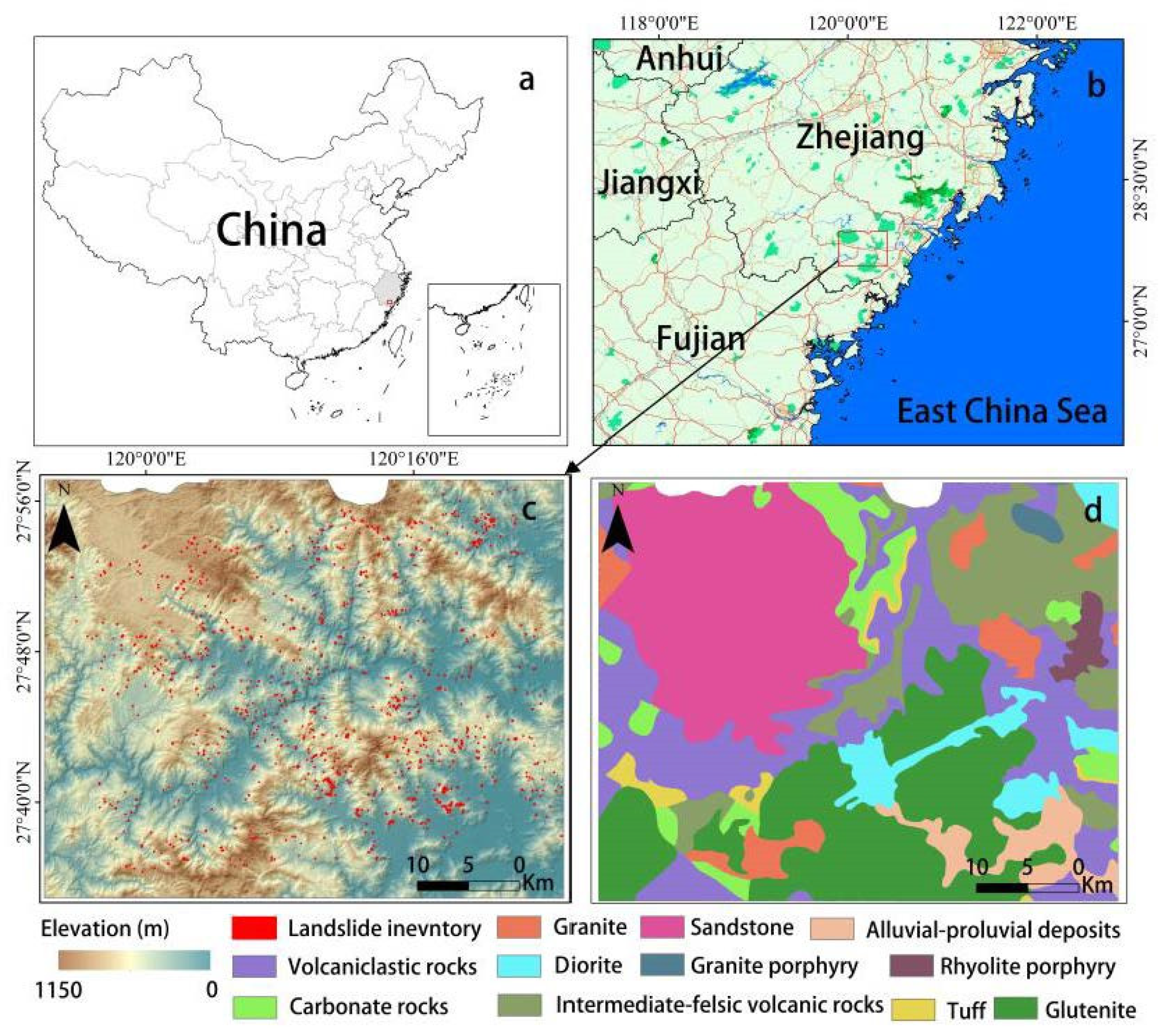
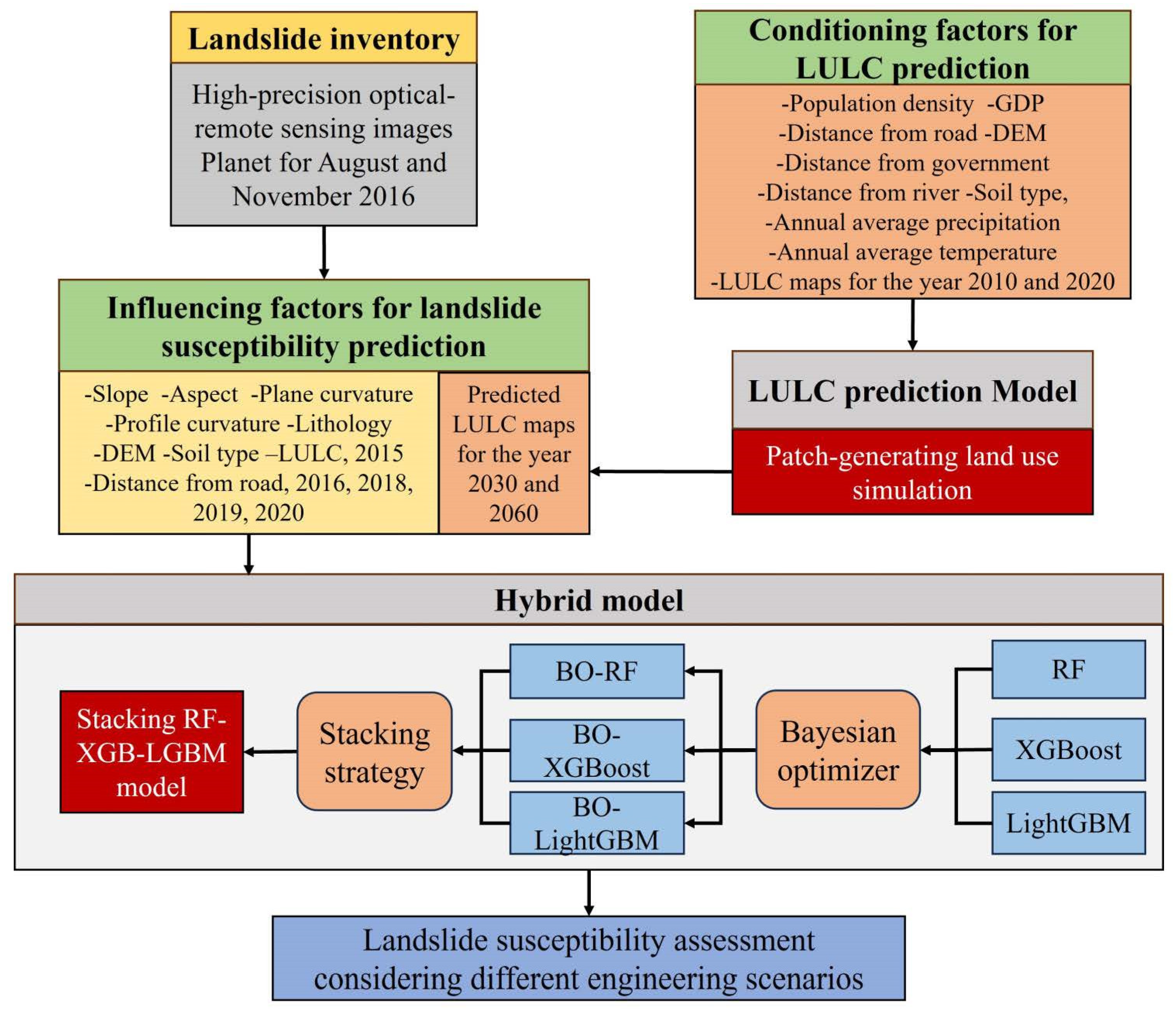
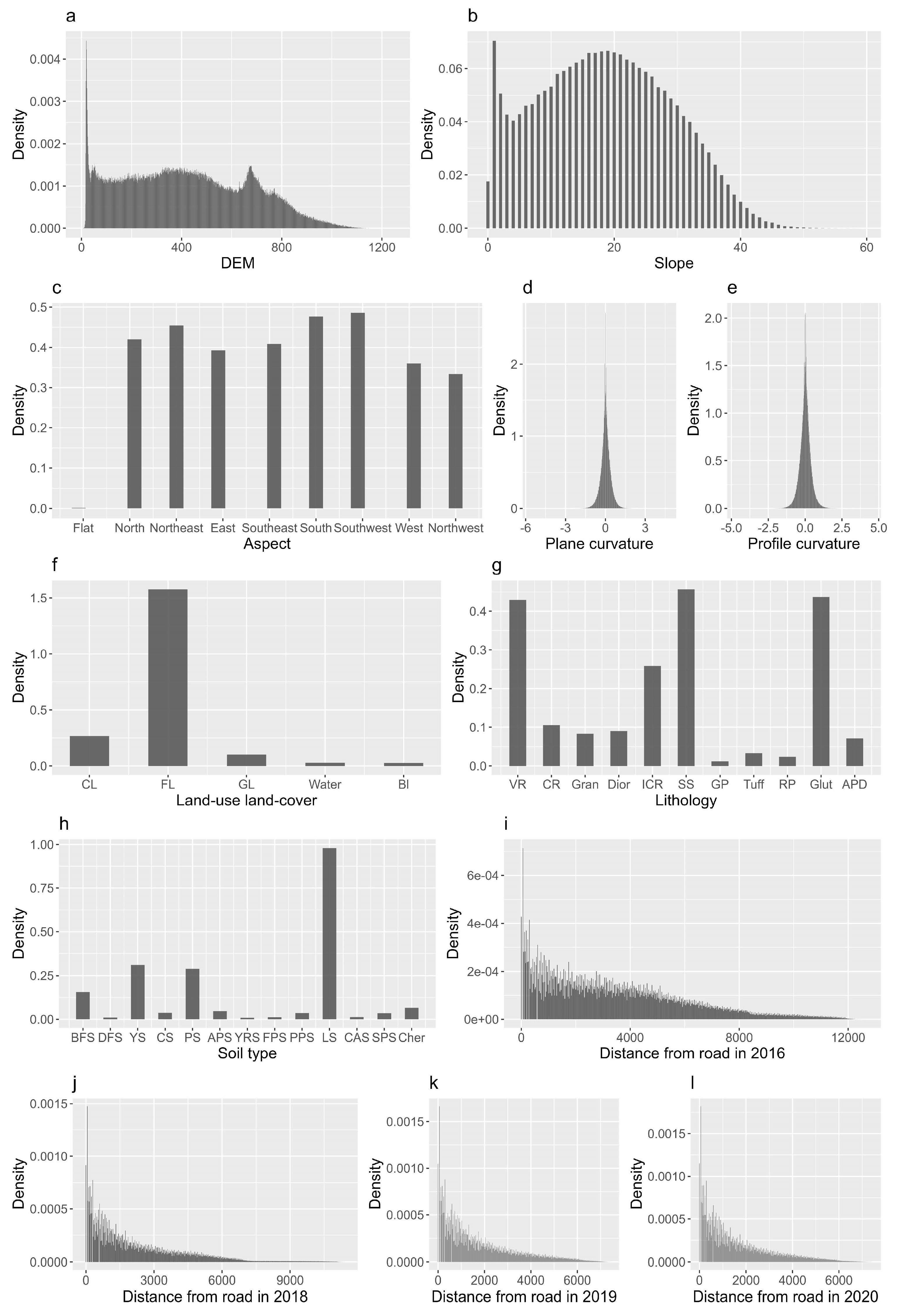
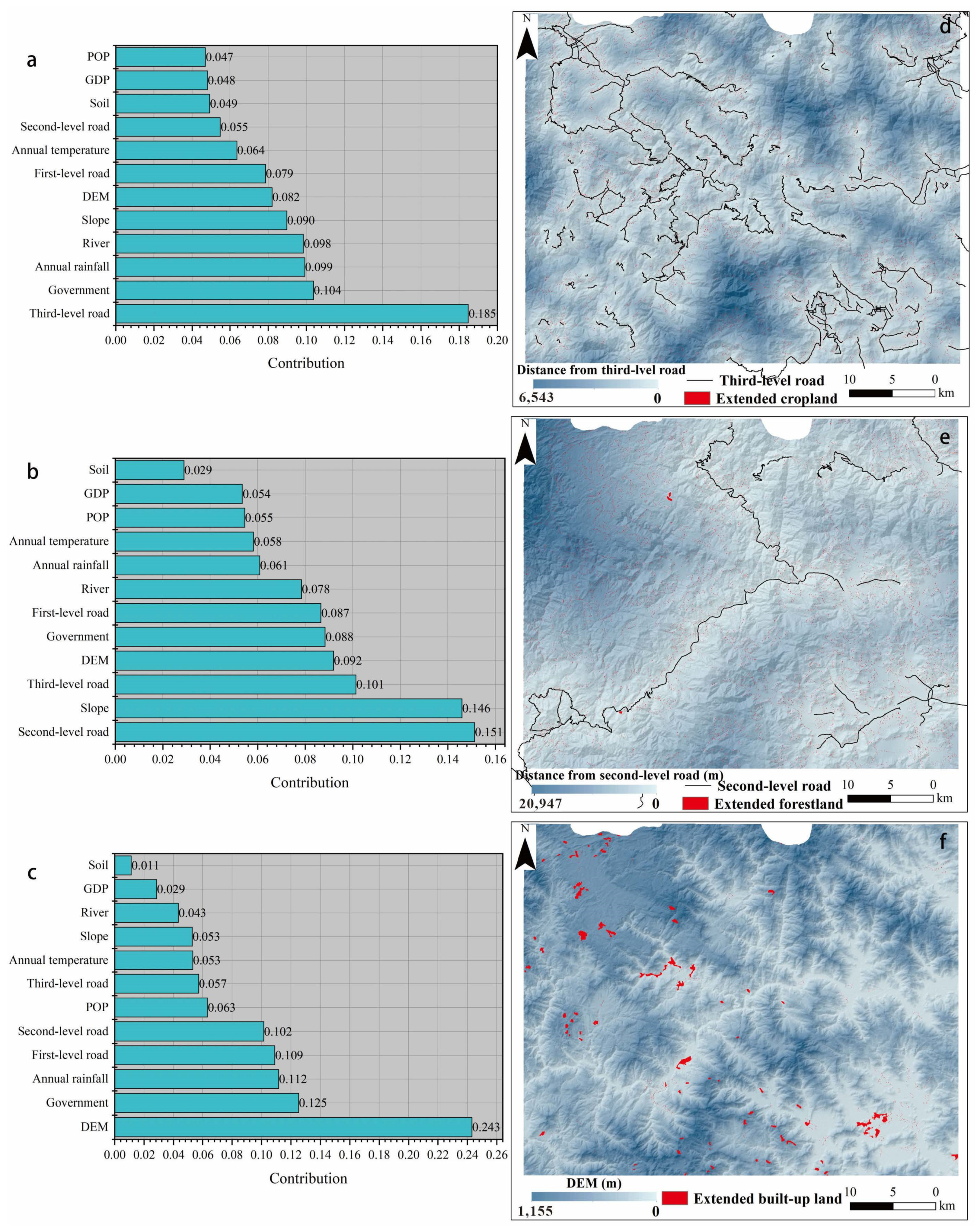
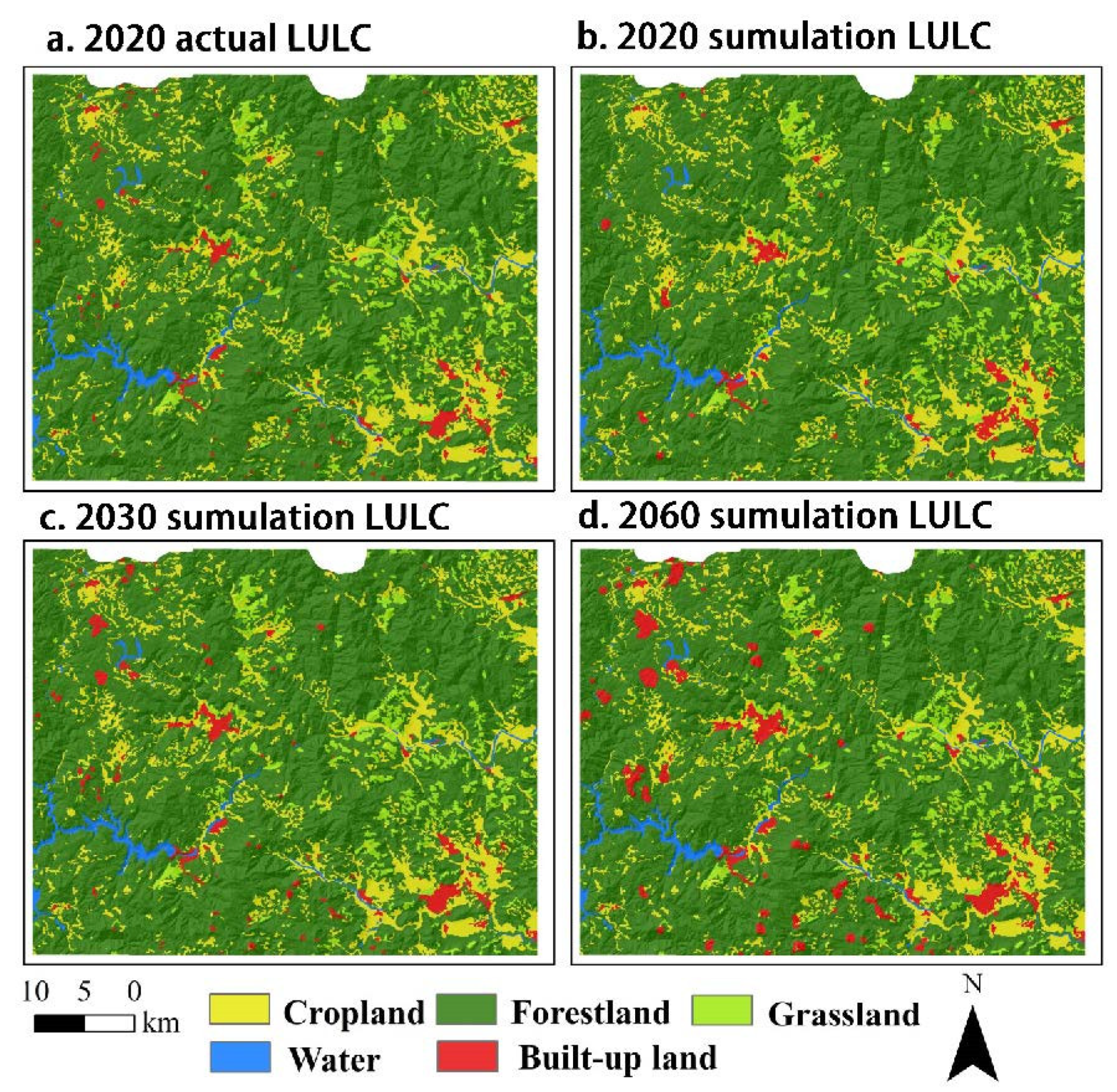
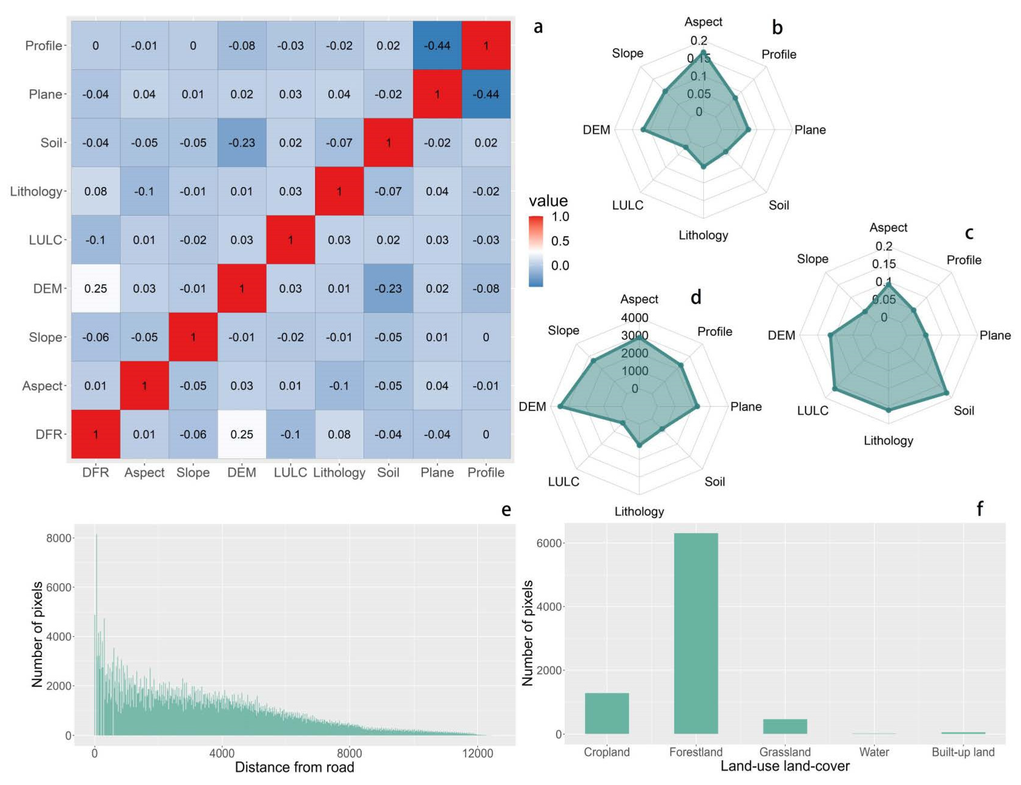
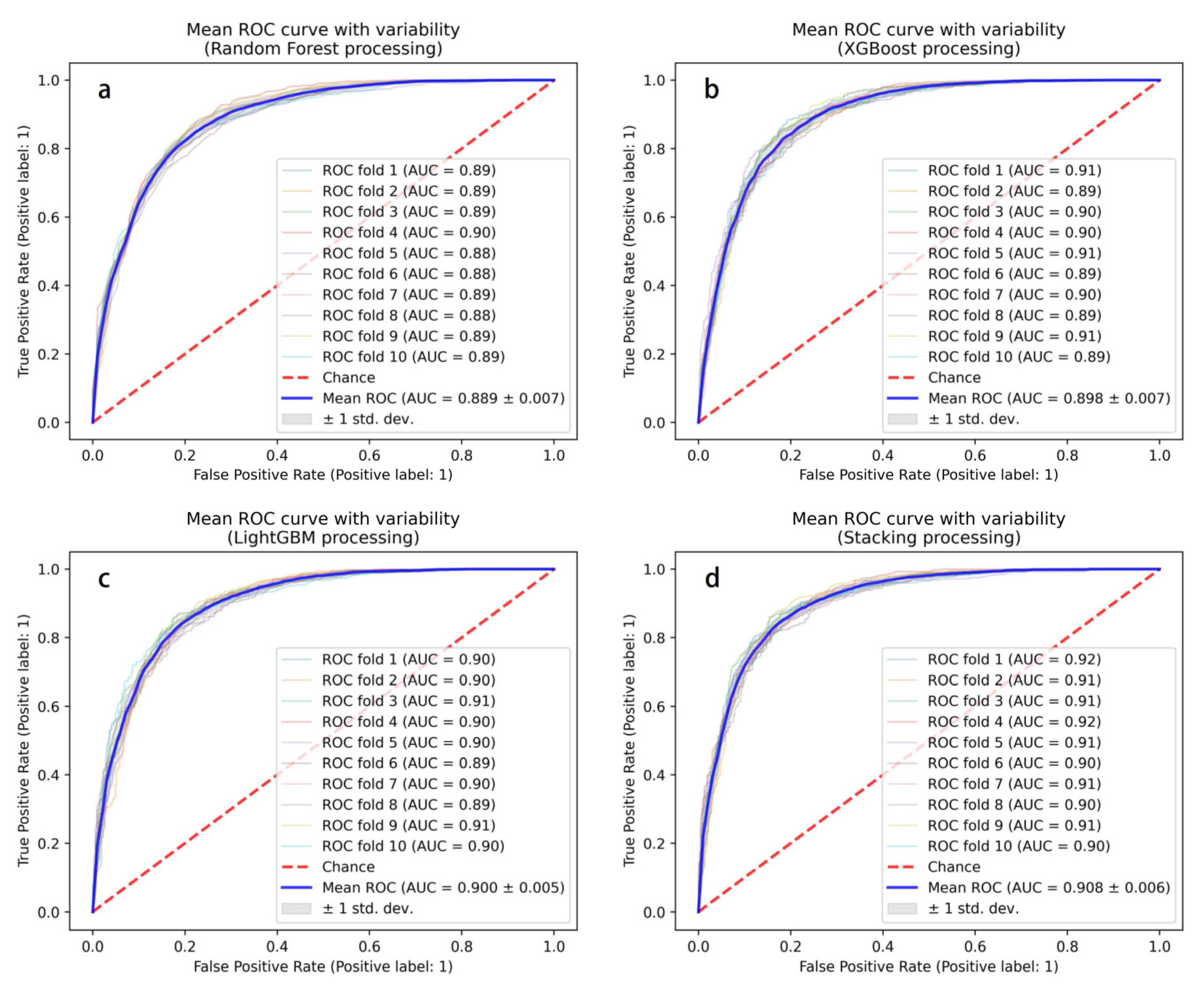
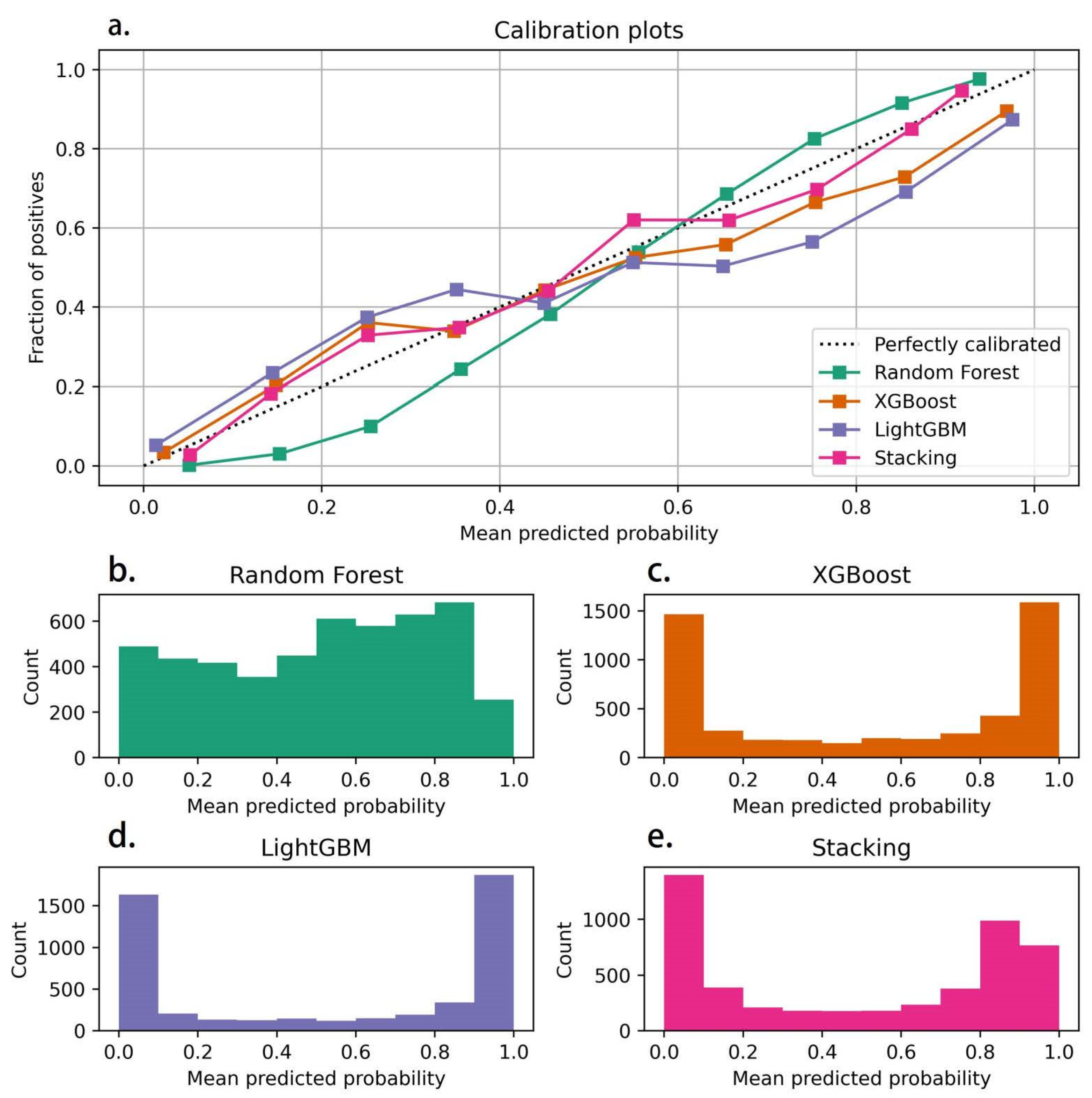
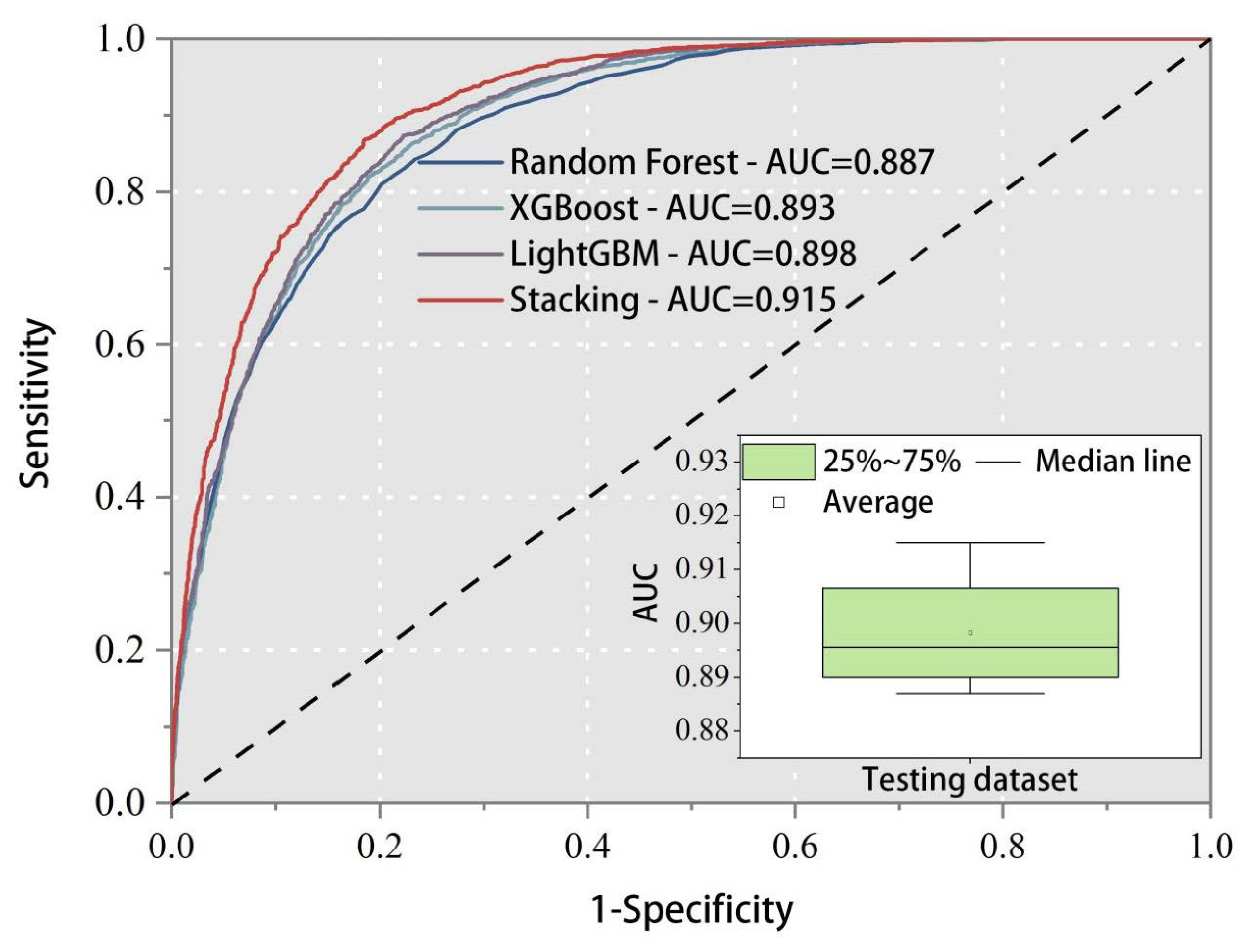
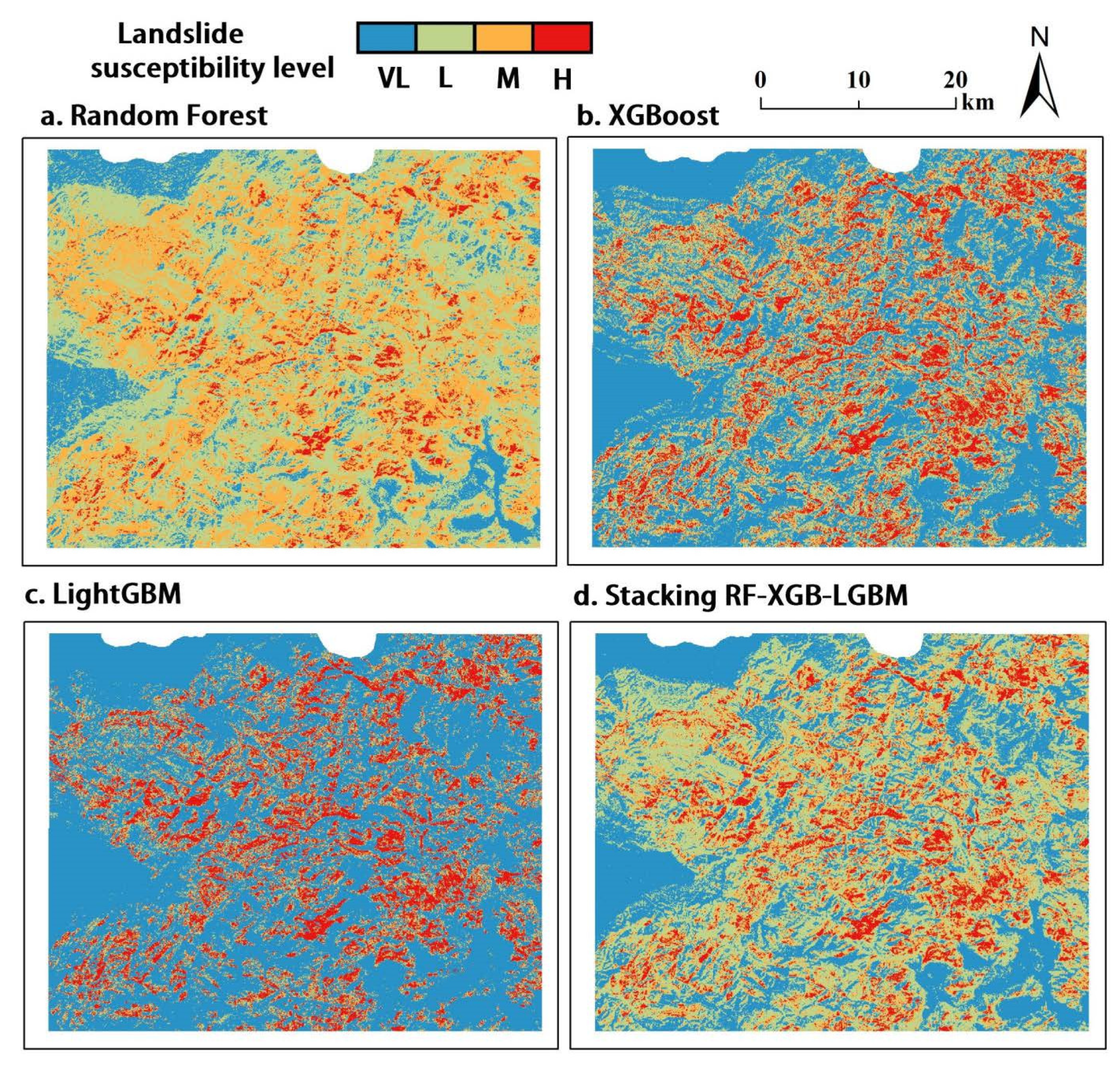
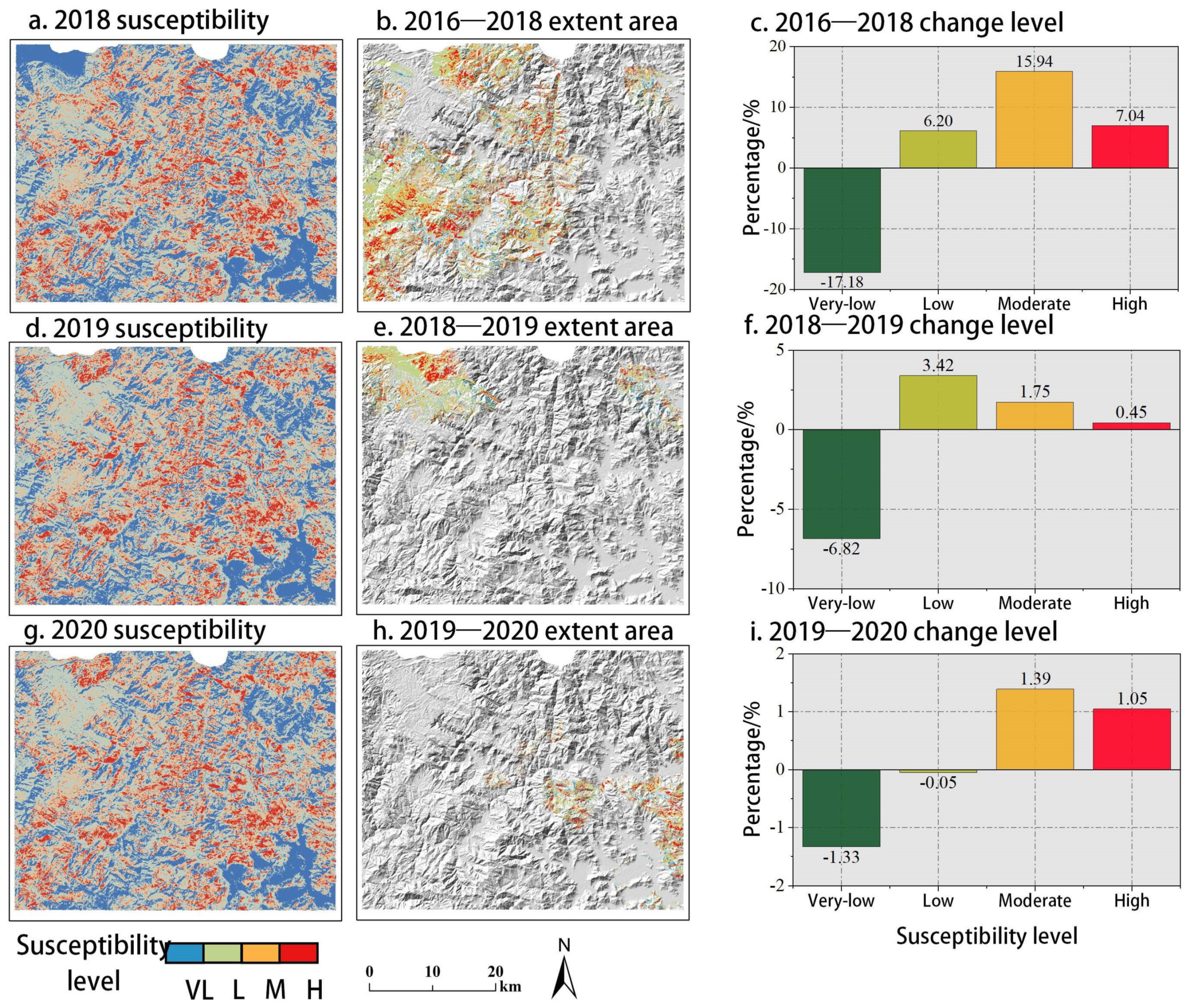
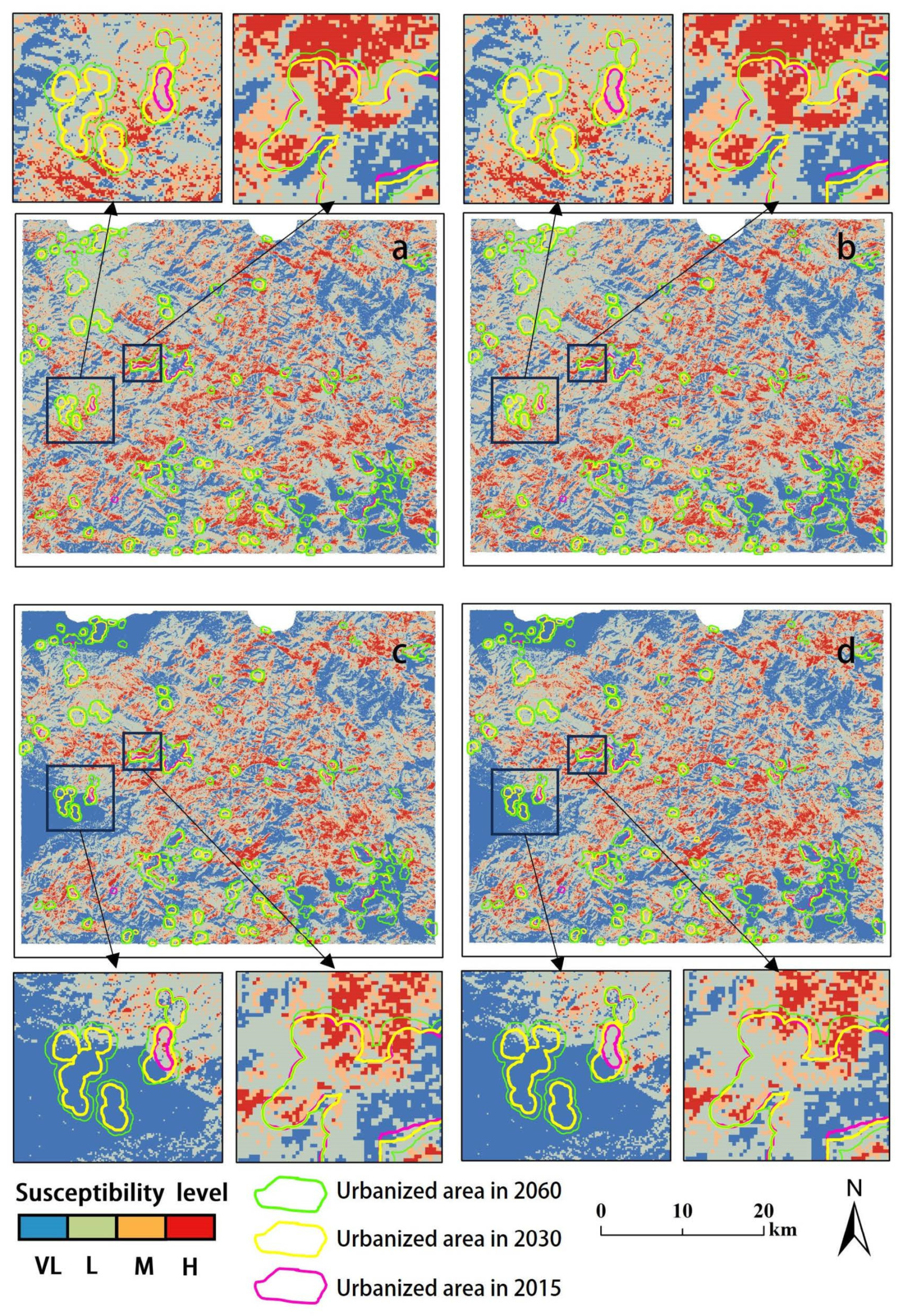
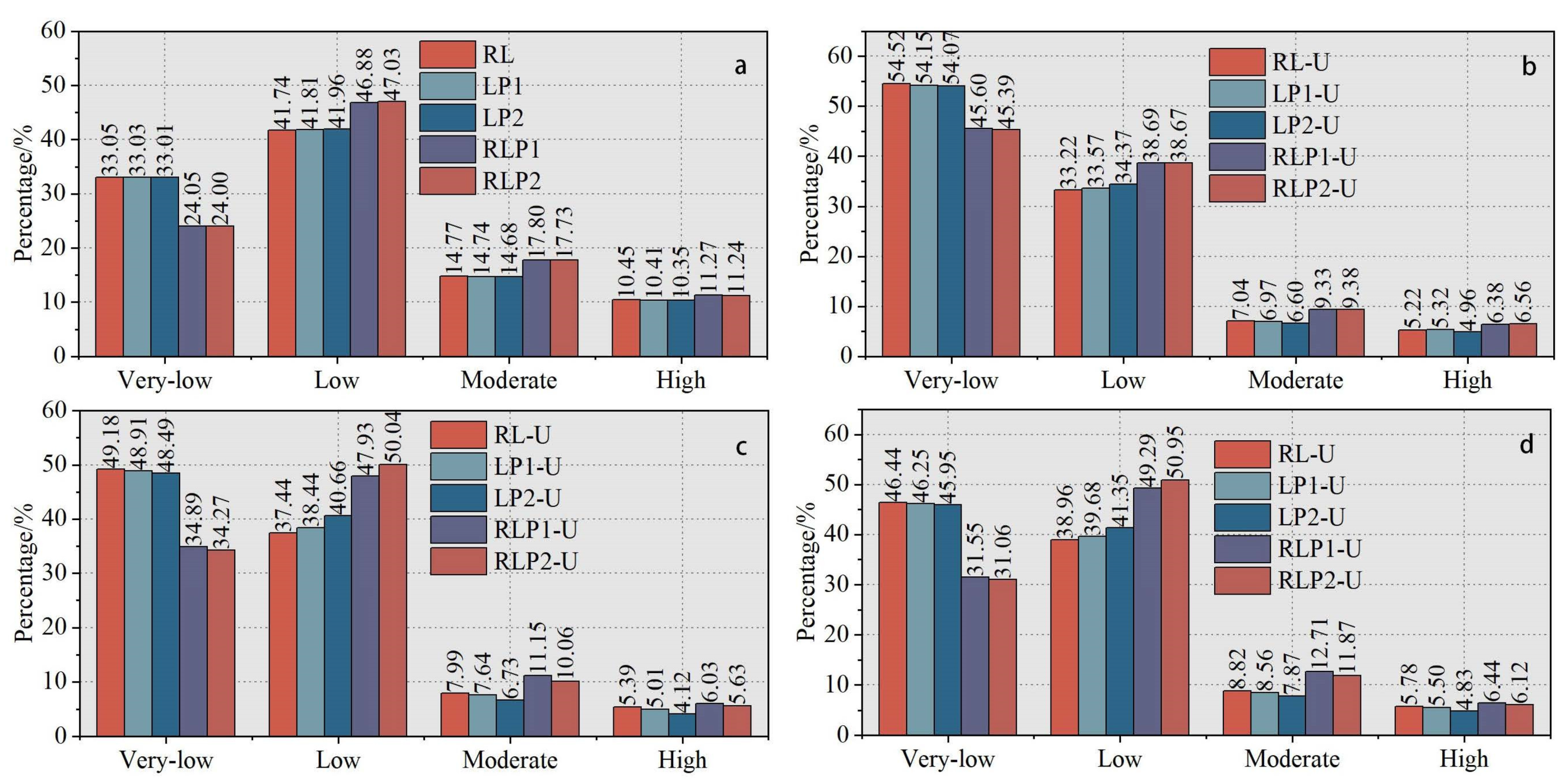
Table 1.
Land-use simulation data source table.
| Data Type | Name | Year | Spatial Resolution | Sources |
|---|---|---|---|---|
| Land-use land-cover data | China’s Multi-Period Land Use Land Cover Remote Sensing Monitoring Dataset | 2010 | 30 m | Data Center for Resources and Environmental Sciences, Chinese Academy of Sciences (https://www.resdc.cn, 20 November 2022) |
| 2015 | 30 m | |||
| 2020 | 30 m | |||
| Socio-economic data | Population density | 2019 | 1 km | |
| GDP | 2019 | 1 km | ||
| Distance from first-class road | 2020 | 30 m | OpenStreetMap (www.openstreetmap.org, 20 November 2022) | |
| Distance from second-class road | 30 m | |||
| Distance from third-class road | 30 m | |||
| Distance from government | 30 m | |||
| Climate-environmental data | Distance from river | 30 m | ||
| Soil type | 1995 | 30 m | Data Center for Resources and Environmental Sciences, Chinese Academy of Sciences (https://www.resdc.cn, 20 November 2022) | |
| Annual average precipitation | 2020 | 1 km | ||
| Annual average temperature | 2020 | 1 km | ||
| DEM | / | 12.5 m | ASF Data Search (https://search.asf.alaska.edu, 20 November 2022) |
Table 2.
Land-use conversion scenario matrix.
| Cropland | Forestland | Grassland | Water | Built-Up Land | |
|---|---|---|---|---|---|
| Cropland | 1 | 1 | 1 | 0 | 1 |
| Forestland | 1 | 1 | 1 | 0 | 1 |
| Grassland | 1 | 1 | 1 | 0 | 1 |
| Water | 0 | 0 | 0 | 1 | 0 |
| Built-up land | 0 | 0 | 0 | 0 | 1 |
Table 3.
Hyper-parameters of three ensemble models.
| Random Forest | XGBoost | LightGBM | |||
|---|---|---|---|---|---|
| N_estimators: (0, 200, 1) | |||||
| Max_depth: (1, 100, 1) | |||||
| Min_sample_split | (3, 30, 1) | Lr: (0.1, 1, 0.1) | |||
| Min_samples_leaf | (3, 30, 1) | Subsample: (0.1, 1, 0.1) | |||
| / | / | Colsample_bytree | (0.1, 1, 0.1) | Num_leaves | (50, 150, 1) |
| / | / | Colsample_bylevel | (0.1, 1, 0.1) | Min_split_gain | (0, 5, 1) |
| / | / | Colsample_bynode | (0.1, 1, 0.1) | Min_child_samples | (10, 50, 1) |
Table 4.
Areas of land-use land-cover types from 2010 to 2020 (km2).
| Land-Use Land-Cover Types | 2010 | 2015 | 2020 |
|---|---|---|---|
| Grassland | 104.67 | 104.301 | 104.809 |
| Cropland | 281.178 | 275.602 | 275.147 |
| Built-up land | 22.2111 | 27.592 | 35.654 |
| Forestland | 1629.896 | 1630.45 | 1622.306 |
| Water | 29.616 | 29.628 | 29.654 |
Table 5.
Transfer matrix and neighborhood weights from 2010 to 2018 (km2).
| 2010 | 2020 | ||||||
|---|---|---|---|---|---|---|---|
| Grassland | Cropland | Built-Up Land | Forestland | Water | Sum | Transferred Out | |
| Grassland | 98.820 | 0.435 | 0.241 | 5.153 | 0.022 | 104.670 | 5.850 |
| Cropland | 0.463 | 260.451 | 5.990 | 13.876 | 0.399 | 281.178 | 20.727 |
| Built-up land | 0.048 | 0.470 | 21.093 | 0.547 | 0.053 | 22.211 | 1.118 |
| Forestland | 5.456 | 13.391 | 8.280 | 1601.660 | 1.110 | 1629.897 | 28.237 |
| Water | 0.023 | 0.401 | 0.050 | 1.071 | 28.071 | 29.616 | 1.545 |
| Sum | 104.810 | 275.147 | 35.654 | 1622.307 | 29.654 | 2067.572 | 5.850 |
| Transferred in | 5.989 | 14.696 | 14.561 | 20.647 | 1.583 | / | / |
| Extended area | 0.139 | 6.031 | 13.443 | 7.590 | 0.038 | / | / |
| Neighborhood weights | 0.1 | 0.447 | 0.9 | 0.563 | 0.1 | / | / |
Table 6.
Optimized parameters of ensemble models.
| Random Forest | XGBoost | LightGBM | |||
|---|---|---|---|---|---|
| N_estimators | 199 | 50 | 200 | ||
| Max_depth | 39 | 32 | 27 | ||
| Min_sample_split | 3 | Lr | 0.5 | 0.3 | |
| Min_samples_leaf | 3 | Subsample | 1.0 | 0.2 | |
| / | / | Colsample_bytree | 0.7 | Num_leaves | 100 |
| / | / | Colsample_bylevel | 0.7 | Min_split_gain | 0 |
| / | / | Colsample_bynode | 1.0 | Min_child_samples | 12 |
Table 7.
Engineering scenarios of different road network and LULC maps.
| Description | Scenarios | Road Network | LULC | |
|---|---|---|---|---|
| All area | Urbanized area | |||
| Basic Condition | RL | RL-U | 2016 | 2015 |
| Short-Term Forecasting | RL1 | RL1-U | 2018 | |
| RL2 | RL2-U | 2019 | ||
| RL3 | RL3-U | 2020 | ||
| Combined Changes | RLP1 | RLP1-U | Predicted 2030 | |
| RLP2 | RLP2-U | Predicted 2060 | ||
| Land-use Changes Only | LP1 | LP1-U | 2016 | Predicted 2030 |
| LP2 | LP2-U | Predicted 2060 | ||
Table 8.
Influence of road network change on the susceptibility level in urban areas.
| Susceptibility Level | Number of Pixels | |||
|---|---|---|---|---|
| RL-U | RL-U1 | RL-U2 | RL-U3 | |
| Very-low | 11,840 | 11,029 | 10,568 | 10,423 |
| Low | 7215 | 7684 | 7994 | 8020 |
| Moderate | 1529 | 1754 | 1845 | 1940 |
| High | 1134 | 1251 | 1311 | 1335 |
Disclaimer/Publisher’s Note: The statements, opinions and data contained in all publications are solely those of the individual author(s) and contributor(s) and not of MDPI and/or the editor(s). MDPI and/or the editor(s) disclaim responsibility for any injury to people or property resulting from any ideas, methods, instructions or products referred to in the content. |
© 2023 by the authors. Licensee MDPI, Basel, Switzerland. This article is an open access article distributed under the terms and conditions of the Creative Commons Attribution (CC BY) license (https://creativecommons.org/licenses/by/4.0/).
Share and Cite
MDPI and ACS Style
Zeng, T.; Guo, Z.; Wang, L.; Jin, B.; Wu, F.; Guo, R. Tempo-Spatial Landslide Susceptibility Assessment from the Perspective of Human Engineering Activity. Remote Sens. 2023, 15, 4111. https://doi.org/10.3390/rs15164111
AMA Style
Zeng T, Guo Z, Wang L, Jin B, Wu F, Guo R. Tempo-Spatial Landslide Susceptibility Assessment from the Perspective of Human Engineering Activity. Remote Sensing. 2023; 15(16):4111. https://doi.org/10.3390/rs15164111
Chicago/Turabian StyleZeng, Taorui, Zizheng Guo, Linfeng Wang, Bijing Jin, Fayou Wu, and Rujun Guo. 2023. "Tempo-Spatial Landslide Susceptibility Assessment from the Perspective of Human Engineering Activity" Remote Sensing 15, no. 16: 4111. https://doi.org/10.3390/rs15164111
Note that from the first issue of 2016, this journal uses article numbers instead of page numbers. See further details here.