Quantifying the Loss of Coral from a Bleaching Event Using Underwater Photogrammetry and AI-Assisted Image Segmentation

Abstract

Detecting the impacts of natural and anthropogenic disturbances that cause declines in organisms or changes in community composition has long been a focus of ecology. However, a tradeoff often exists between the spatial extent over which relevant data can be collected, and the resolution of those data. Recent advances in underwater photogrammetry, as well as computer vision and machine learning tools that employ artificial intelligence (AI), offer potential solutions with which to resolve this tradeoff. Here, we coupled a rigorous photogrammetric survey method with novel AI-assisted image segmentation software in order to quantify the impact of a coral bleaching event on a tropical reef, both at an ecologically meaningful spatial scale and with high spatial resolution. In addition to outlining our workflow, we highlight three key results: (1) dramatic changes in the three-dimensional surface areas of live and dead coral, as well as the ratio of live to dead colonies before and after bleaching; (2) a size-dependent pattern of mortality in bleached corals, where the largest corals were disproportionately affected, and (3) a significantly greater decline in the surface area of live coral, as revealed by our approximation of the 3D shape compared to the more standard planar area (2D) approach. The technique of photogrammetry allows us to turn 2D images into approximate 3D models in a flexible and efficient way. Increasing the resolution, accuracy, spatial extent, and efficiency with which we can quantify effects of disturbances will improve our ability to understand the ecological consequences that cascade from small to large scales, as well as allow more informed decisions to be made regarding the mitigation of undesired impacts.

1. Introduction

Natural and anthropogenic disturbance events can cause mass declines in the foundational species of ecosystems. Detecting and quantifying the impact of these events is a critical focus of ecology [1], but doing so in a way that achieves results at ecologically meaningful scales can be difficult [2]. The effort required to collect high-resolution data constrains the areal and temporal extent that can feasibly be surveyed, limiting our ability to fully assess the ecological consequences of disturbance. This is especially the case for shallow marine ecosystems [3]. Fortunately, advances in underwater photogrammetry techniques and computer vision tools, assisted by artificial intelligence (AI), provide solutions to resolve this tradeoff.

Coral reef ecosystems illustrate the need for and challenges associated with high-resolution change detection. These highly productive systems host a staggering level of biodiversity that relies on reef-building corals [4]. The benthic communities of tropical reefs are difficult to quantify at all relevant spatial and temporal scales. In situ visual surveys can be relatively rapid and cost-effective, but they often yield coarse estimates of organismal cover. Conversely, the manual annotation of images can produce high-resolution data but the process is comparatively time- and labor-intensive [5,6]. This is a growing issue because coral reefs are increasingly threatened by disturbances that cause persistent and expansive declines in reef-building corals, the organisms that form the structural foundations of these ecosystems [7]. Specifically, episodes of coral bleaching, associated with periods of elevated ocean temperatures, can kill corals on landscape scales, and these events are increasing in both intensity and frequency on a global scale [8,9,10,11,12]. This underscores the importance of developing methods that can be used to accurately and efficiently assess the severity of disturbances that kill coral in order to better understand their cascading impacts [13,14,15,16,17,18,19].

A suite of innovative tools and technologies has been utilized to map coral reef communities. Underwater photogrammetry, for example, is increasingly used to quantify the structural attributes of coral reefs. Large-scale efforts have been undertaken to create extensive maps of these ecosystems at high spatial resolutions using photogrammetry [5,20,21]. Generally, extracting metrics of the physical attributes of a reef (e.g., surface rugosity or roughness) from these maps is relatively straightforward. However, efficiently extracting biological metrics, such as cover of benthic organisms (e.g., coral or algae), can be more complicated and time-consuming [6]. A widely implemented approach is image segmentation—the scaled measurement and annotation of objects within an image [22,23,24,25]. This form of image analysis is generally used to estimate metrics, including percentage cover of benthic flora and fauna, via the 2D areal footprint of organisms in a given area. Although image segmentation has been used on orthophotomosaics [26,27], the effort to do so manually constrains the ability to scale up the technique in space and time. Thus, a bottleneck exists that prevents the extraction of biological metrics, like the growth and survival of individual coral colonies, both at large spatial scales and with high temporal resolution [6]. This limits our ability to track meaningful changes in the benthic community composition on coral reefs over time and thereby inhibits our understanding of how fine-scale changes in the populations or communities of benthic organisms might translate into landscape-scale impacts. Fortunately, innovations in machine learning provide a promising solution to this challenge.

Through AI-assisted image segmentation, the labor required to measure and identify ecologically relevant objects, such as the sizes and identities of coral colonies, can be automated, thus decreasing the time required for this task and increasing the amount of information that can potentially be acquired. Deep learning methods have been implemented to greatly increase the efficiency with which complex or irregular objects, such as coral colonies, can be segmented from images [28,29]. Additionally, they enable reef-scale changes in rugosity and structure to be detected over time [30]. We build on this work here, outlining a framework that combines a rigorous underwater photogrammetry technique [31] with novel, AI-assisted image segmentation software, TagLab (version 2023.5.16, [32]), to quantify the impact of a major coral bleaching event on an ecologically meaningful tract of South Pacific coral reef with high spatial resolution (Figure 1). Specifically, we aimed to: (1) quantify the amount of live coral loss that resulted from the bleaching event with higher accuracy and precision; (2) explore size-dependent patterns of coral mortality; and (3) compare the estimates from our approach with more widely used methods of quantifying changes in coral cover. Using the workflow outlined in Figure 2, we detected a dramatic loss in the amount of live coral on the reef and a reorganization in the size structure of an important coral population through size-dependent mortality of bleached corals. Lastly, we found that using approximated 3D surface area as a metric when estimating coral cover enabled us to capture a significantly greater loss of live coral compared to using 2D planar area, a metric that has been widely used to measure coral size in images.

2. Materials and Methods

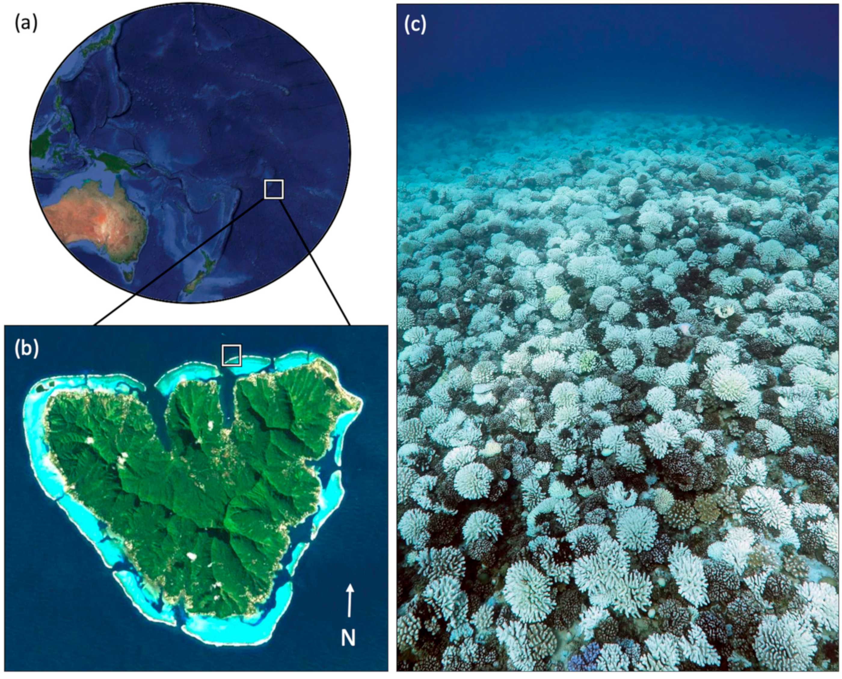
2.1. Site Description

We conducted our study on Moorea, French Polynesia (17°30′S, 149°50′W), a high volcanic island in the South Pacific Ocean with steep fore-reef slopes that extend offshore to a barrier reef that surrounds the island’s ~60 km perimeter (Figure 1a,b). The Moorea Coral Reef Long Term Ecological Research program (MCR LTER, https://mcr.lternet.edu) has been collecting time series data on coral reef communities of Moorea since 2005, performing photogrammetric surveys of several reef tracts at about 10 m depth on the north shore fore reef annually since 2017. In April 2019, a prolonged period of elevated sea surface temperatures triggered a major coral bleaching event that resulted in significant coral mortality on the fore reef ([33]; Figure 1c). Our photogrammetric surveys spanned this major disturbance, providing an opportunity to evaluate the utility of our AI-assisted approach to quantifying change. We focused our analyses on two time points (photogrammetric epochs): August 2018 (epoch 1), about 8 months before the bleaching event when live coral cover was at an all-time high, and August 2019 (epoch 2), about 4 months after the bleaching event once there had been significant deaths of live coral.

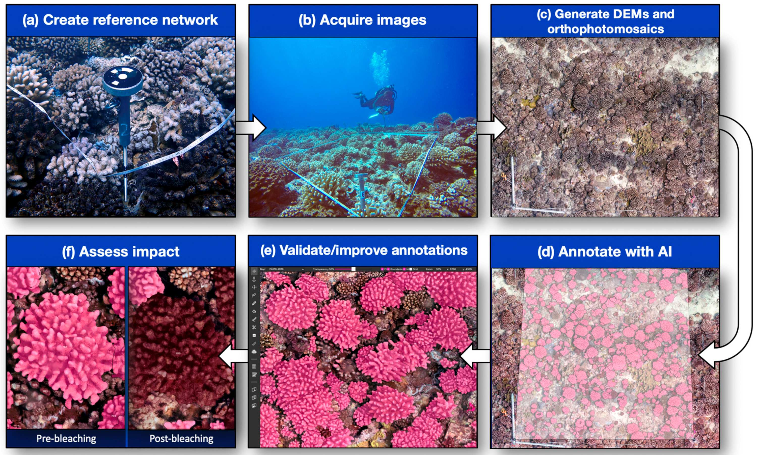
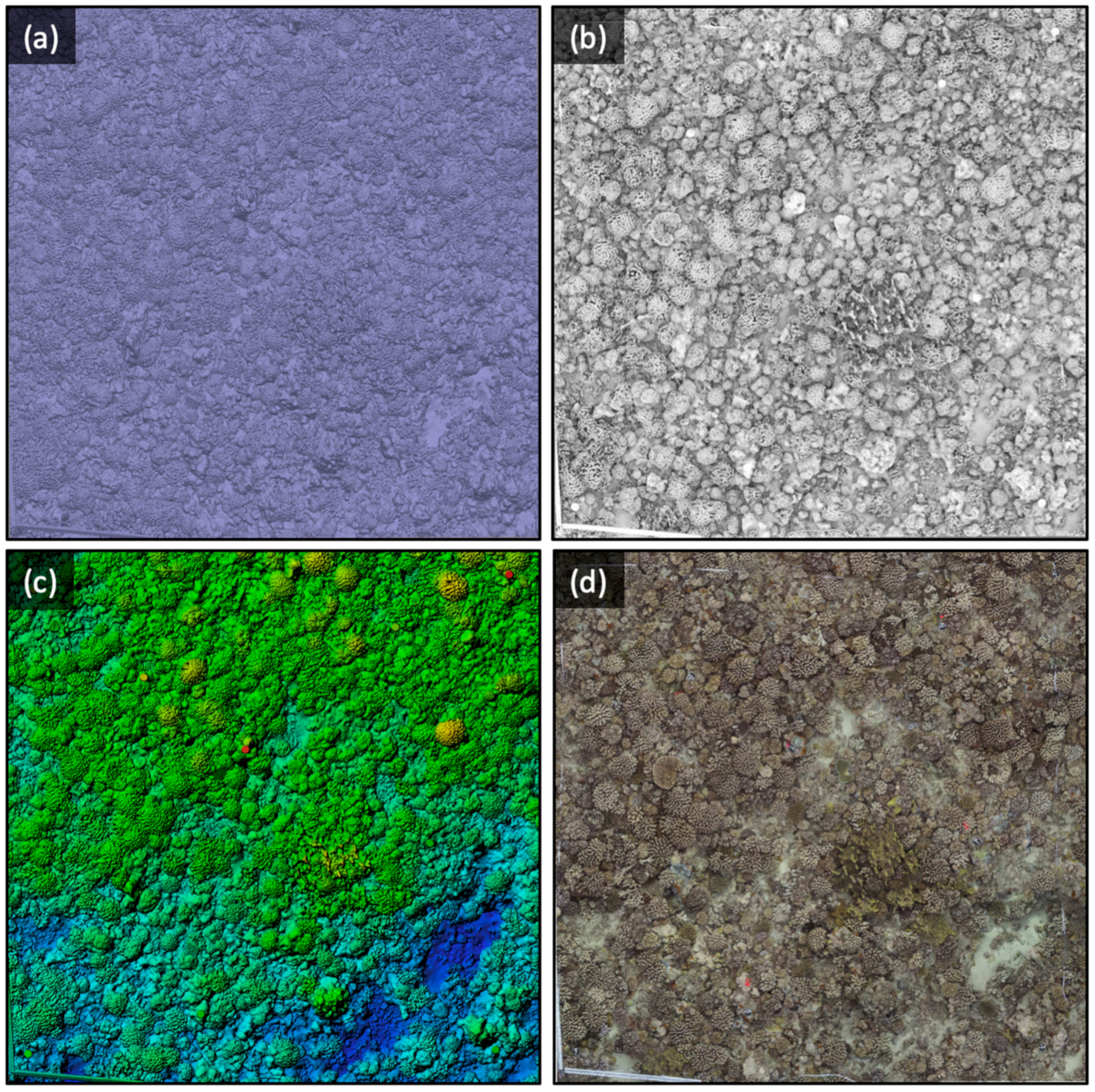
2.2. Reference Network Establishment, Image Acquisition, and Orthophotomosaic Generation

The first step in the workflow (Figure 2) is to establish a series of geodetic networks, that is, permanent, fixed reference points in the reef substrate from which the reference network can be measured. Creating a permanent and reliable reference network is critical to both scaling the photogrammetric models and registering multiple models in space and time. For our network, the reference points were established by SCUBA divers who drilled holes into the primary reef substrate and affixed anchors (using underwater epoxy), into which specially designed photogrammetry targets could be installed and then removed during each sampling event (Figure 2a). The horizontal and vertical distances between all targets are then measured with sub-centimeter precision (see [31,34]). The 5 reef plots used in this study each have a footprint of about 25 m² (5 × 5 m) and a geodetic reference network that was established in 2017. From the reference network measurements for each plot, we estimate a set of coordinates that are used to establish a temporally stable reference system. This allows us to co-register the photogrammetric surveys and products from the different epochs (see [31]).

Once the reference network is in place, SCUBA divers systematically photograph the reef (Figure 2b). As the diver swims, downward-pointing and oblique photographs are taken at a fixed distance above the reef (1–2 m) at a consistent rate in order to achieve at least an 80% overlap (but generally > 90%) between consecutive images. Divers were able to maintain a consistent distance above the reef while acquiring images using the depth gauge on their dive computers [31,34]. The diver completes a series of parallel passes along the length of a reef plot, and then a series of passes perpendicular to the first. Finally, a series of oblique (45-degree angle to the reef) photographs are taken around the perimeter of the plot. To minimize the variation in the light incidence on the reef, which is caused by temporal and environmental factors, we photographed our plots during the same time of year (August, the austral winter) and during the same time of day (between late morning and early afternoon). In total, 500–800 images were taken of each plot during each epoch (see [31]). Images were acquired in their raw format and white balance adjustment was performed using color checkers distributed in the measurement area before converting the images into the highest-quality JPG format in order to reproduce a more accurate color spectrum [31]. This allows us to extensively adjust the lighting and color of the acquired images, despite environmental conditions (e.g., cloud cover, water turbidity, depth, etc.) that might cause variation in these attributes. This step is fundamental in our protocol as color fidelity is critical for the human identification of marine organisms. It also facilitates the training and implementation of the automated semantic segmentation process described below in Section 2.3.

The final step of our photogrammetric process is constructing digital elevation models (DEMs) and orthorectified photomosaics (orthophotomosaics, for short) of each plot (Figure 3). We would like to clarify, however, that the three-dimensional information obtained from DEMs is of the single-valued form, z = f(x,y), and hence is an approximation (i.e., ‘2.5D’) of the true three-dimensional shape of the reef. All photogrammetric models and orthophotomosaics were generated using Agisoft Metashape (version 2.0), with an average ground resolution of less than 1 mm (i.e., pixel size: <1 × 1 mm) and a discrepancy among reference coordinates of a few millimeters [31,34].

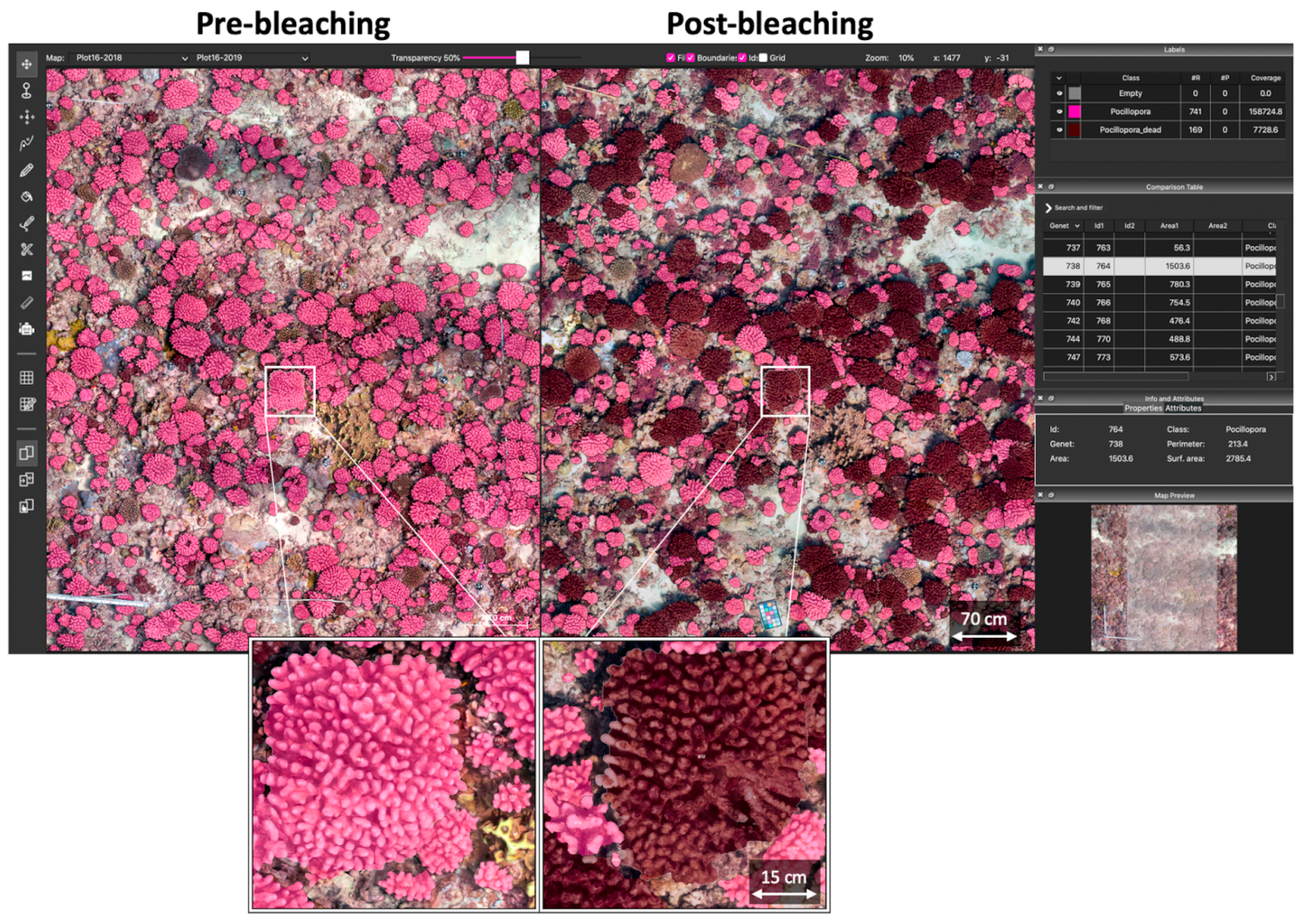
2.3. AI-Assisted Image Segmentation and Manual Validation and Editing

Semantic segmentation involves the detection and partitioning of an image into different subdivisions based on their class. We employed TagLab (https://taglab.isti.cnr.it, [32]), an open-source, AI-powered, and interactive image segmentation software designed for coral reef habitats, to annotate and measure corals in our orthophotomosaics (Figure 2d and Figure 4). TagLab enables pixel-wise, accurate, and scale-aware labeling and analysis of orthophotomosaics. This software also facilitates time series analysis when multiple images of a site are available from different epochs. For example, it is possible to automatically track temporal changes of individual objects (e.g., growth, shrinkage, or death of coral colonies) in sequential orthophotomosaics of the same site when the objects are co-registered (Figure 4, inset panels). Further, TagLab enables a user to create custom classifiers for the automatic recognition of objects of interest via the creation of a training dataset. Building the training dataset utilizes semi-automatic segmentation, in which a human operator manually identifies and labels colonies after using AI-assisted tools to outline coral colony borders. For example, the user only needs to indicate the four most extreme points of a colony border rather than trace the entire colony. This and other semi-automatic segmentation tools greatly expedite the creation of the training dataset, after which fully automatic segmentation can be used. In this study, 2 of the 10 orthophotomosaics (the same plot from both epochs) that we produced were annotated semi-automatically in order to build the training dataset for the fully automatic classifier, which was then used to segment the remaining 8 orthophotomosaics. TagLab is available to download from Github: https://github.com/cnr-isti-vclab/TagLab (see [32] for more detail on the software’s mechanics).

A human operator should always validate automatic segmentations visually (Figure 2e). Then, depending on the desired metric or level of accuracy, the operator can correct mistakes made during the automatic classification by manually correcting any poorly predicted colony borders or mislabeled objects. This will require additional human labor and processing time. In this study, once the training dataset had been used to build the fully automatic classifier, we took further action to validate the accuracy of the automatic classifier and improve the quality of the automatic segmentations. Because we were interested in exploring patterns based on individual coral colony size, we manually divided segmentations that enclosed multiple, overlapping or adjacent coral colonies of the same taxon. However, if a user is interested solely in the total areal coverage by different types of objects (e.g., live and dead corals), a minimum of further editing would likely be required. Lastly, we modified the TagLab software for this study in order to approximate the 3D metrics of reef organisms. Previously, TagLab did not support the loading or analysis of DEMs, but only three-channel (RGB) images. The software was modified to be able to layer the RGB images onto their respective DEMs in order to extract 3D approximations of coral colony (and other) surface areas.

2.4. Analyses and Impact Assessment

Due to the dominance of corals from the genus Pocillopora inhabiting the reefs we studied (>90% of coral colonies present), and the relative scarcity of other taxa, we focused our analyses on changes in Pocillopora corals. Using the automatically generated, manually corrected segmentations, we analyzed several metrics of live and dead coral cover to estimate the changes driven by the bleaching event (Figure 2f). First, we excluded all segmentations < 2 cm², as these were too small for a human observer to reliably identify. Next, we calculated the total proportion of colonies that were alive or dead before and after the bleaching event in order to understand how the ratio of live to dead colonies changed in response to this disturbance. To quantify the magnitude of change in live and dead coral areas from before to after bleaching, we summed the total 3D surface areas (estimated from digital elevation models (DEMs) of the photogrammetric models) of live and dead colonies for all 5 plots in each epoch (pre-bleaching: 2018, post-bleaching: 2019), and then averaged the results across replicate plots within an epoch.

To explore patterns of size-dependent mortality after bleaching, we sorted the live and dead colonies into size classes (based on the approximated 3D surface area of a coral colony) and compared the abundances of these classes before and after the bleaching event. The thresholds for the size classes were based on the quartiles of colony sizes for live corals before the bleaching event (i.e., the size structure of the pre-bleaching population). We rounded the size thresholds slightly to create clean cut-offs between classes. To create just three size classes (Small, Medium, and Large), the middle two quartiles were combined for the Medium size class, as these two quartiles behaved similarly to one another through time. The final size classes used were: <100 cm² (Small), 100–400 cm² (Medium), and >400 cm² (Large). Because larger colonies were more scarce than smaller ones, the ‘Large’ class contained a much wider range in terms of size (401–3487 cm²) than the two smaller classes. Lastly, we applied these size classes to the dead coral colonies to assess the mortality of corals based on colony size.

Finally, we compared the estimated loss of live coral cover after the bleaching event using two different metrics of coral surface area: approximated 3D surface area derived from the DEMs, and 2D planar area derived from the areas enclosed by the perimeters of segmented regions. A 2D planar area is commonly used in studies of coral reefs to estimate the areal footprints of corals and other organisms within an image, which are then used as proxies for coral colony size. To test whether the approximated 3D metric captured a greater magnitude of coral decline after bleaching compared to the 2D metric, we ran an analysis of covariance (ANCOVA) on live coral surface area as a function of area metrics (approximated as 3D or 2D) and epoch (pre-bleaching: 2018, post-bleaching: 2019). All analyses were performed in R (version 4.0.0, [35]) and RStudio (version 2022.12.0.353, [36]) using the Tidyverse package [37], and visualizations utilized colors from Manu: NZ Bird Colour Palettes [38].

3. Results

3.1. Automatic Segmentation and Manual Validation/Improvement

After training a custom classifier on two orthophotomosaics of the same plot (one image from epoch 1 pre-bleaching: 2018; one from epoch 2 post-bleaching: 2019), the fully automatic classification correctly classified 93% of pixels (each ~1 mm) for living Pocillopora. This result is comparable to the performance of a human operator and is the maximum accuracy generally achievable [32]. The classification accuracy for dead coral, however, was lower, with 70% of pixels correctly classified. There were two reasons for this. First, dead coral often resembles the primary reef substrate and therefore was sometimes misclassified as background reef. Second, there was a relatively low representation of dead coral in the two orthophotomosaics used for the training dataset, as dead corals were prevalent only in the post-bleaching image, which could be rectified by additional training. Nonetheless, the automatic classifier was able to segment the corals in an entire orthophotomosaic in a matter of minutes, a task that would have taken a human operator many hours to complete manually.

While the automatic classifier was highly accurate in classifying pixels as live or dead coral, it did not yet have the ability to distinguish well between colonies that have abutting borders. Therefore, to obtain information on sizes and numbers of colonies, further manual division of the segmentations by a human was required. Before cropping our orthophotomosaics down to designated working areas (to standardize the areas surveyed), and before removing segmentations < 2 cm² in area, 2060 segmentations of live coral were completed automatically for the orthophotomosaics of the pre-bleaching epoch. These segmentations were further divided manually by a human observer into 4366 live colonies. For the post-bleaching epoch, 2426 segmentations were completed automatically and were then manually divided further into 3181 live colonies. The number of dead coral colonies was nearly identical between the automatic and manual segmentations for the pre-bleaching epoch (1288 compared to 1289, respectively). However, for the 2019 epoch, manual division increased the number of dead colonies from 1471 to 2077. After manually correcting all segmentations, removing segmentations < 2 cm², and standardizing the results to the designated working areas for the plots, the total number of corals (live + dead) was 4306 in the pre-bleaching epoch and 4015 in the post-bleaching epoch. Manually dividing the automatically segmented colonies added only about one hour per orthophotomosaic to the overall time required for processing the images.

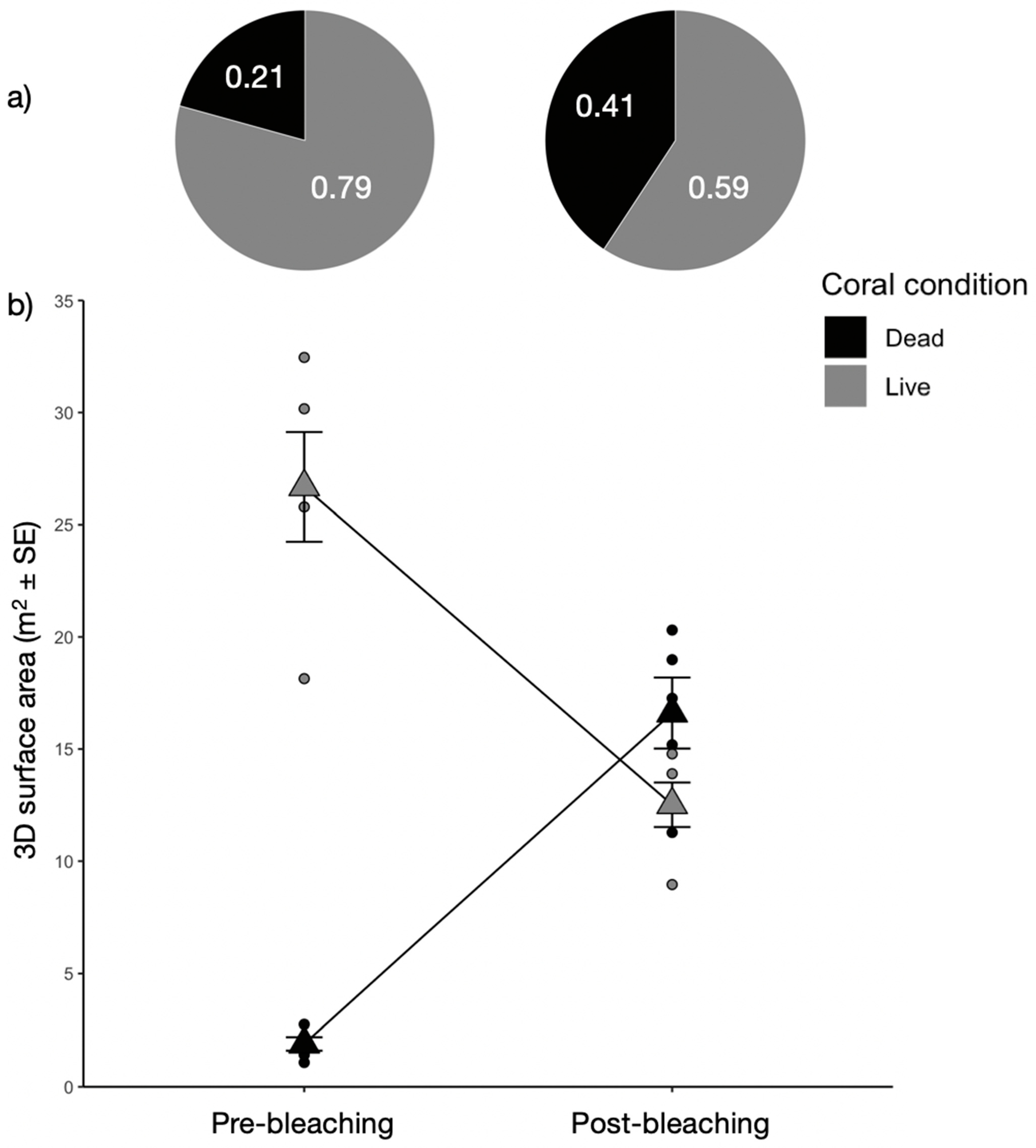
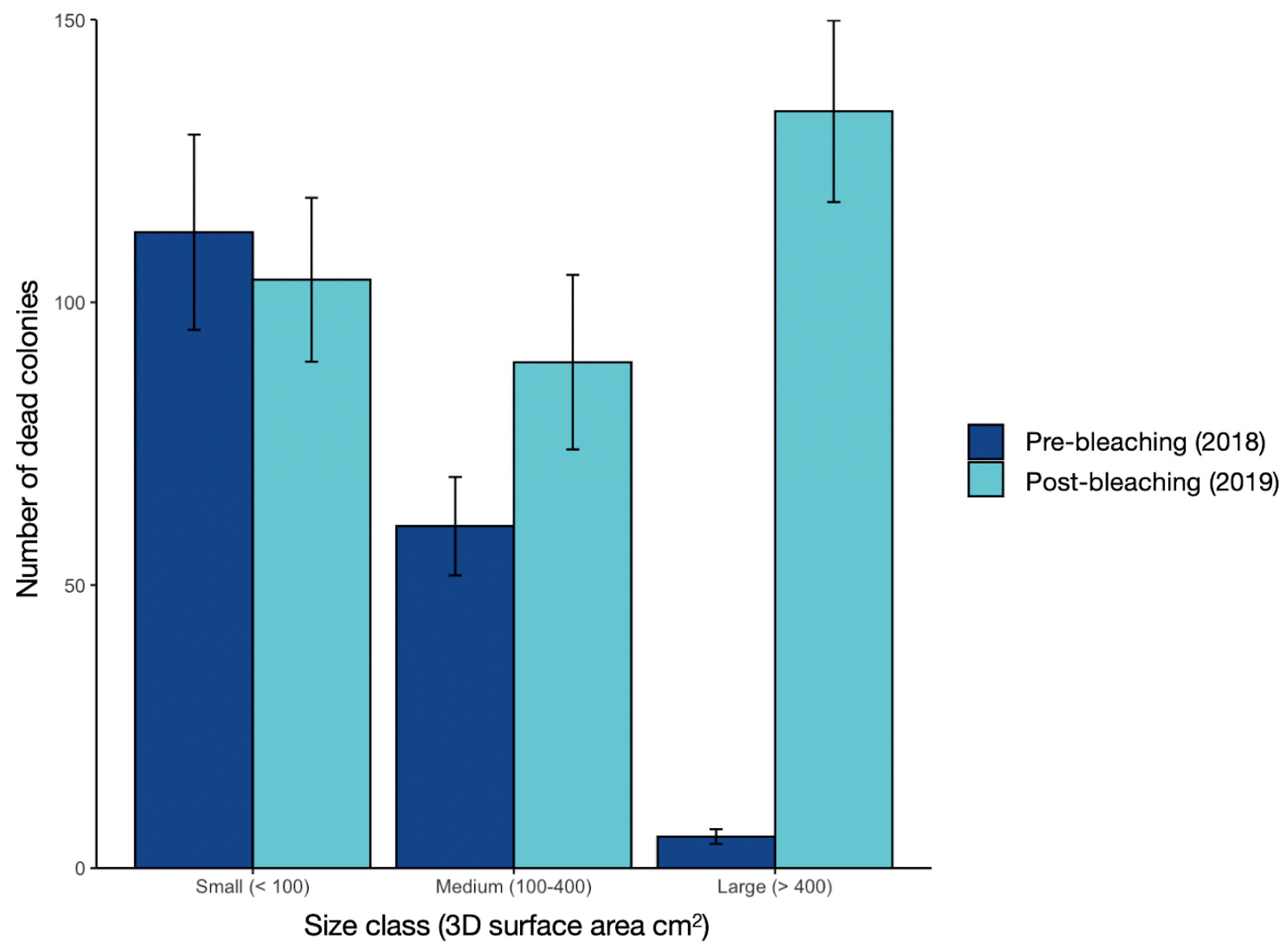
3.2. Changes in Colony Numbers, Approximated 3D Surface Areas, and Size Structure of Corals

As expected, the proportions of live and dead coral colonies changed substantially from before to after the bleaching event (Figure 5a). Of the 4306 colonies measured across all 5 plots before bleaching (within designated working areas), roughly 21% (904) of these were dead. However, this proportion nearly doubled following the bleaching event, after which 41% (1,646) of the 4015 colonies measured were classified as dead. Our assessment of changes in the approximated 3D surface areas of live and dead corals at the plot scale (~25 m²) before and after bleaching revealed even more dramatic changes (Figure 5b). After bleaching, the approximated 3D surface area of live coral decreased by more than half, from 26.7 (±2.4) m² to 12.5 (±1.0) m² (means ± SE), respectively. By contrast, the total surface area of dead coral increased over eightfold, from 1.9 (±0.3) m² to 16.6 (±1.6) m², and surpassed the total amount of coral surface area that remained alive after the bleaching event.

We explored size-dependent relationships of coral mortality and found striking differences among size classes in their response to bleaching (Figure 6). The number of colonies in the largest size class of dead coral (>400 cm²) increased 24-fold after the bleaching event, from 5.6 (±1.3) dead colonies per plot (mean ± SE) before bleaching to 133.8 (±16.0) dead colonies afterward. The Medium size class (100–400 cm²) showed a much more modest 1.3-fold increase, from 60.4 (±8.7) colonies before bleaching to 89.4 (±15.4) colonies after. Lastly, the smallest size class showed no statistical differences in the mean number of dead corals per plot from before to after the bleaching event. This size-dependent pattern in mortality corroborates our observation that the change in surface area of live and dead coral was markedly higher than the change in the proportion of live and dead colonies. This could be explained by the fact that larger colonies contributed disproportionately more to reef coverage than smaller colonies did.

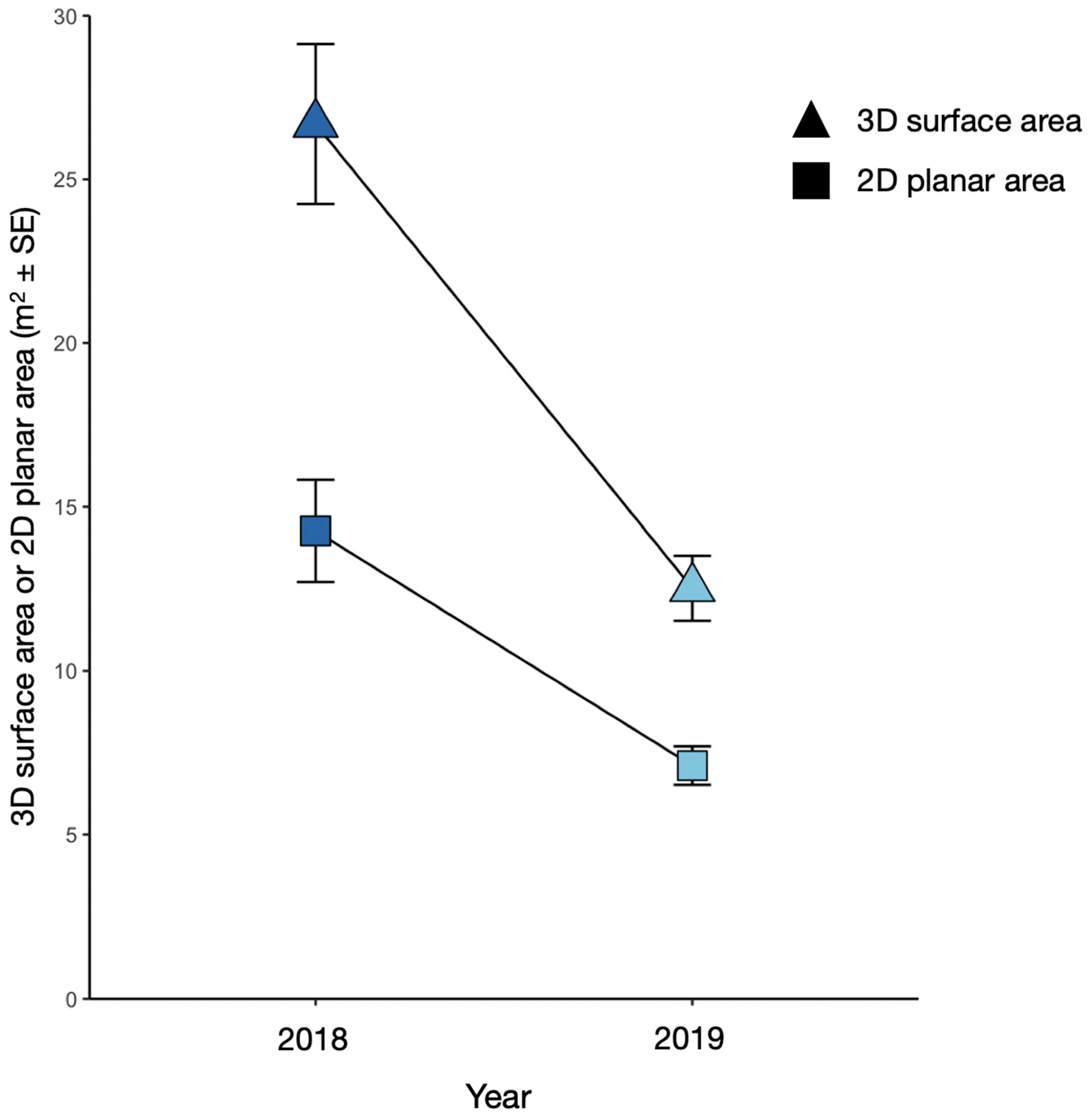
3.3. Comparison of Approximated 3D Surface Area with 2D Planar Area

Our comparison of the approximated 3D surface area estimates with 2D planar area estimates of live corals showed, unsurprisingly, that the 3D metric estimated far greater amounts of live coral area within a time period than the 2D metric (triangles compared to squares in Figure 7). More importantly, the approximated 3D metric revealed a significantly greater loss rate of live coral than the 2D metric (slopes of the relationships in Figure 7 differ; ANCOVA F1, 0.05 = 5.05, p = 0.03; see Appendix A,

Table A1. Results of Analysis of Covariance (ANCOVA) testing the effect of using 2D vs. 3D measures of live coral area to compare changes in cover of live coral before and after a major bleaching event.

Source	DF	Sum of Squares	Mean Square	F Value	Pr > F
Model	3	1027.918483	342.639494	28.18	<0.0001
Error	16	194.538179	12.158636
Corrected Total	19	1222.456661
R-Square		Coeff Var	Root MSE		Area Mean
0.840863		23.02680	3.486924		15.14290
Source	DF	Type I SS	Mean Square	F Value	Pr > F
Area_Type	1	397.6459238	397.6459238	32.70	<0.0001
Time_Point	1	568.8996018	568.8996018	46.79	<0.0001
Time_Point *Area_Type	1	61.3729571	61.3729571	5.05	0.0391
Source	DF	Type III SS	Mean Square	F Value	Pr > F
Area_Type	1	188.7322881	188.7322881	15.52	0.0012
Time_Point	1	568.8996018	568.8996018	46.79	<0.0001
Time_Point *Area_Type	1	61.3729571	61.3729571	5.05	0.0391

).

4. Discussion

4.1. Quantification of the Coral Bleaching Event

Assessing the ecological impacts of natural and anthropogenic disturbances is increasingly important as these events become more common and severe. Therefore, innovative tools and reliable methods are needed to accurately quantify changes in populations and communities of organisms affected by these disturbances. This is especially important for shallow subtidal ecosystems such as coral reefs, which are becoming increasingly threatened by more frequent and severe bleaching events [8,9,10,11,12]. Here, we outlined a novel method that combined underwater photogrammetry with AI-assisted image segmentation software in order to rapidly and accurately quantify the impact of a major coral bleaching event on a tropical reef. We showed significant changes to the composition of this reef at both the coral colony and landscape scales. The use of an approximated 3D metric to quantify coral, as facilitated by the tools and techniques we described, provided a more accurate estimate of the amount of coral present and the rate of loss due to a coral mortality event compared to the more commonly used 2D metric.

The workflow described here not only enables a more accurate quantification of coral loss over ecologically meaningful spatial scales (Figure 5), but it also provides the ability to characterize a colony’s size-specific pattern of mortality. For Pocillopora, the prominent taxon of coral in the system, the largest colonies were disproportionately affected by the bleaching event in that the number of dead colonies in the largest size class increased by an order of magnitude greater than that seen for smaller-sized colonies (Figure 6). This pattern aligns with other field studies of coral bleaching in Moorea [39,40,41] and energetic modeling of corals [42], which have all found size-specific variation in the susceptibility of Pocillopora colonies to bleaching and in their subsequent mortality. The disproportionate loss of larger Pocillopora colonies also explains the greater effect we observed on the change in coral cover (Figure 5b) compared to the smaller change in proportions of live and dead colonies (Figure 5a).

Many studies of coral reefs have implemented manual tracing of coral colonies to estimate their areal footprint as a 2D surface, which is used as a proxy for colony size [22,23,24,25,43]. By approximating the 3D surface areas of corals, we captured a loss rate of live coral that was significantly greater than that estimated by 2D planar area (Figure 7). A previous study [44] that explored the relationship between 2D and 3D estimates of total surface area of single coral colonies revealed scaling relationships that depended on coral morphology, leading the authors to conclude that the labor-intensive nature of measuring corals in 3D may be avoided by converting 2D measurements into 3D metrics to quantify change over ecologically meaningful spatial scales in the field. Our coupling of a rigorous photogrammetric survey method with novel, open-access and AI-assisted image segmentation software (TagLab) enabled the direct 3D approximation of both the surface area of coral skeletons and semantic segmentation of co-located coral colonies with high resolutions over large scales. This AI-assisted approach enabled us to estimate absolute changes in live and dead coral cover on the reef with a realistic level of effort. In turn, this could improve estimates of how disturbance will modify important ecological processes and services that corals provide, such as reef metabolism and habitat provisioning [45,46], enabling ecologists to better predict the cascading ecological consequences of disturbance [13,14,15,16,17,18,19].

4.2. Advantages to Our Approach

Our photogrammetric approach allowed us to quantify changes in live and dead coral cover over spatial scales of 10s of square meters with sub-centimeter resolution and accuracy [31,32]. From an ecological standpoint, the use of a fixed geodetic reference network, as we described here, provides several benefits compared to more commonly used photogrammetric survey techniques. First, the reference network acts to set a robust, three-dimensional scale for measuring objects (such as coral colonies) within an orthophotomosaic. Second, the reference network enables users to georeference their orthophotomosaics and therefore align multiple orthophotomosaics of the same site that were taken at different times (epochs). This facilitates highly precise spatiotemporal comparisons that can yield highly accurate time series estimations of important biological variables. Third, the reference network provides users with a means of estimating the error margins of their measurements, allowing them to assess whether changes in biological variables through time (such as growth or loss of corals) are statistically significant [31,34].

When coupled with AI, the high volumes of information contained in large orthophotomosaics can be processed efficiently. With the use of TagLab, we were able to rapidly extract large amounts of high spatial resolution data from the orthophotomosaics produced by our photogrammetric approach (Figure 4). Automating the annotation of these orthophotomosaics substantially reduced the processing time compared to annotations completed manually [3,32]. Not only were the automated annotations highly accurate compared to those completed by humans, but they can also be improved further through manually editing or additional data and training. Further, once a desired level of accuracy is achieved in training the program, the process of extracting data from orthophotomosaics can be completed by personnel with less taxonomic or ecological expertise. Automating the highly time-intensive task of measuring corals within photographs, such as we have shown here, can boost our capability to monitor and detect changes in highly threatened ecosystems like coral reefs.

4.3. Caveats to Our Approach

Several opportunities exist for improvement of our workflow. With regard to the photogrammetric process, the establishment of an underwater fixed reference network can be a challenging and labor-intensive task. New tools based on the integration of inertial measurement units (IMUs) and depth sensors [47,48], however, are being developed in order to reduce the number of measurements needed between fixed reference points—in particular, the vertical distances between fixed reference points, which are the most difficult to measure. With regard to the AI-assisted segmentation process, several issues arose that required manual intervention. First, while the automatic classifier was highly accurate in classifying live coral and reasonably accurate in classifying dead coral, it had difficulty differentiating between colonies in the same semantic category when they shared borders or overlapped with one another. This is understandable, as this task was difficult even for human observers due to the high density of abutting, congeneric coral colonies on the reefs we studied. If a user is interested in colony-level changes (as opposed to total, reef-scale changes in coral cover), some additional labor may be required to manually separate colonies if colony density is high on the reef being studied. Second, the automatic classifier failed to classify live and dead coral correctly in a small minority of cases (<10%). This could be attributable to the image quality for those particular colonies, or the relatively small training dataset we used (the program was trained on only two orthophotomosaics, one of which contained relatively few dead coral colonies). Nonetheless, TagLab performed impressively with respect to quantifying live and dead coral cover, its automatic segmentations can be continually improved with further training or manual editing, and it will likely become a widely used tool in the study and monitoring of coral reef ecosystems.

4.4. Future Directions

There are several avenues to build on the research we have presented here, some of which are already being explored. First, researchers in our group are currently developing techniques to perform segmentation on 3D point clouds, which will further enhance the accuracy of measuring the 3D surface areas of complex structures like coral colonies using photogrammetric methods. Additionally, we are exploring the incorporation of multispectral sensors into underwater drones to facilitate the acquisition and processing of underwater images that can be used for underwater photogrammetry. As for developments regarding TagLab, there are several in progress. First, data from subsequent years following those presented in this study can be used to further train the automatic classifier, making it more robust. We plan to release this trained model to be publicly available. We are also currently refining methods and algorithms to easily track individual objects as they transition between classes, such as a live coral colony that dies wholly or partially between epochs. Further, we are developing an AI-assisted point classification tool that can be used to estimate the cover of organisms and objects that are difficult to measure via currently available tools (e.g., patches of algae). Lastly, the architecture of TagLab will soon transition from using semantic segmentation to panoptic segmentation. This will allow for the quantification of amorphous or indistinct components of the benthos, such as reef substrate or coral rubble.

5. Conclusions

The pace of changing global conditions warrants the development of sophisticated methods and tools that can be used to make informed decisions regarding the management of threatened ecosystems. Here, we have described an integrated underwater photogrammetry and AI-assisted image segmentation methodology for robustly and efficiently quantifying change in coral, the foundation species of tropical reefs. The insights that can be gleaned from this technique are numerous and could enable ecologists to answer questions that may not feasibly be addressed using traditional methods. Further, robust change detection, as we have demonstrated, could prove highly valuable for ecological monitoring efforts by reducing the tradeoff between the areal extent that can be feasibly surveyed and the spatial resolution that can be achieved. Enhancing both the spatial extent and resolution of ecological monitoring will strengthen our ability to forecast how the functioning of vulnerable ecosystems, such as coral reefs, will change in an uncertain future, helping us to mitigate the undesired impacts of disturbance.

References

1. Osenberg, C.W.; Schmitt, R.J. Chapter 1—Detecting Ecological Impacts Caused by Human Activities. In Detecting Ecological Impacts; Schmitt, R.J., Osenberg, C.W., Eds.; Academic Press: San Diego, CA, USA, 1996; pp. 3–16. ISBN 978-0-12-627255-0. [Google Scholar]
2. Solow, A.R. On Detecting Ecological Impacts of Extreme Climate Events and Why It Matters. Philos. Trans. R. Soc. B Biol. Sci. 2017, 372, 20160136. [Google Scholar] [CrossRef] [PubMed]
3. Miller, S.D.; Dubel, A.K.; Adam, T.C.; Cook, D.T.; Holbrook, S.J.; Schmitt, R.J.; Rassweiler, A. Using Machine Learning to Achieve Simultaneous, Georeferenced Surveys of Fish and Benthic Communities on Shallow Coral Reefs. Limnol. Oceanogr. Methods 2023, 21, 451–466. [Google Scholar] [CrossRef]
4. Knowlton, N.; Brainard, R.E.; Fisher, R.; Moews, M.; Plaisance, L.; Caley, M.J. Coral Reef Biodiversity. In Life in the World’s Oceans; McIntyre, A.D., Ed.; Wiley-Blackwell: Oxford, UK, 2010; pp. 65–78. ISBN 978-1-4443-2550-8. [Google Scholar]
5. Urbina-Barreto, I.; Garnier, R.; Elise, S.; Pinel, R.; Dumas, P.; Mahamadaly, V.; Facon, M.; Bureau, S.; Peignon, C.; Quod, J.-P.; et al. Which Method for Which Purpose? A Comparison of Line Intercept Transect and Underwater Photogrammetry Methods for Coral Reef Surveys. Front. Mar. Sci. 2021, 8, 636902. [Google Scholar] [CrossRef]
6. Couch, C.S.; Oliver, T.A.; Suka, R.; Lamirand, M.; Asbury, M.; Amir, C.; Vargas-Ángel, B.; Winston, M.; Huntington, B.; Lichowski, F.; et al. Comparing Coral Colony Surveys From In-Water Observations and Structure-From-Motion Imagery Shows Low Methodological Bias. Front. Mar. Sci. 2021, 8, 647943. [Google Scholar] [CrossRef]
7. Hoegh-Guldberg, O.; Mumby, P.J.; Hooten, A.J.; Steneck, R.S.; Greenfield, P.; Gomez, E.; Harvell, C.D.; Sale, P.F.; Edwards, A.J.; Caldeira, K.; et al. Coral Reefs Under Rapid Climate Change and Ocean Acidification. Science 2007, 318, 1737–1742. [Google Scholar] [CrossRef]
8. Donovan, M.K.; Burkepile, D.E.; Kratochwill, C.; Shlesinger, T.; Sully, S.; Oliver, T.A.; Hodgson, G.; Freiwald, J.; van Woesik, R. Local Conditions Magnify Coral Loss after Marine Heatwaves. Science 2021, 372, 977–980. [Google Scholar] [CrossRef]
9. Hughes, T.P.; Kerry, J.T.; Simpson, T. Large-Scale Bleaching of Corals on the Great Barrier Reef. Ecology 2018, 99, 501. [Google Scholar] [CrossRef]
10. Hughes, T.P.; Kerry, J.T.; Connolly, S.R.; Baird, A.H.; Eakin, C.M.; Heron, S.F.; Hoey, A.S.; Hoogenboom, M.O.; Jacobson, M.; Liu, G.; et al. Ecological Memory Modifies the Cumulative Impact of Recurrent Climate Extremes. Nat. Clim. Chang. 2019, 9, 40–43. [Google Scholar] [CrossRef]
11. Lough, J.M.; Anderson, K.D.; Hughes, T.P. Increasing Thermal Stress for Tropical Coral Reefs: 1871–2017. Sci. Rep. 2018, 8, 6079. [Google Scholar] [CrossRef]
12. Donovan, M.K.; Adam, T.C.; Shantz, A.A.; Speare, K.E.; Munsterman, K.S.; Rice, M.M.; Schmitt, R.J.; Holbrook, S.J.; Burkepile, D.E. Nitrogen Pollution Interacts with Heat Stress to Increase Coral Bleaching across the Seascape. Proc. Natl. Acad. Sci. USA 2020, 117, 5351–5357. [Google Scholar] [CrossRef]
13. Holbrook, S.J.; Schmitt, R.J.; Messmer, V.; Brooks, A.J.; Srinivasan, M.; Munday, P.L.; Jones, G.P. Reef Fishes in Biodiversity Hotspots Are at Greatest Risk from Loss of Coral Species. PLoS ONE 2015, 10, e0124054. [Google Scholar] [CrossRef] [PubMed]
14. Holbrook, S.J.; Schmitt, R.J.; Brooks, A.J. Resistance and Resilience of a Coral Reef Fish Community to Changes in Coral Cover. Mar. Ecol. Prog. Ser. 2008, 371, 263–271. [Google Scholar] [CrossRef]
15. Messmer, V.; Jones, G.P.; Munday, P.L.; Holbrook, S.J.; Schmitt, R.J.; Brooks, A.J. Habitat Biodiversity as a Determinant of Fish Community Structure on Coral Reefs. Ecology 2011, 92, 2285–2298. [Google Scholar] [CrossRef] [PubMed]
16. Han, X.; Adam, T.C.; Schmitt, R.J.; Brooks, A.J.; Holbrook, S.J. Response of Herbivore Functional Groups to Sequential Perturbations in Moorea, French Polynesia. Coral Reefs 2016, 35, 999–1009. [Google Scholar] [CrossRef]
17. Adam, T.C.; Brooks, A.J.; Holbrook, S.J.; Schmitt, R.J.; Washburn, L.; Bernardi, G. How Will Coral Reef Fish Communities Respond to Climate-Driven Disturbances? Insight from Landscape-Scale Perturbations. Oecologia 2014, 176, 285–296. [Google Scholar] [CrossRef] [PubMed]
18. Kopecky, K.L.; Stier, A.C.; Schmitt, R.J.; Holbrook, S.J.; Moeller, H.V. Material Legacies Can Degrade Resilience: Structure-Retaining Disturbances Promote Regime Shifts on Coral Reefs. Ecology 2023, 104, e4006. [Google Scholar] [CrossRef] [PubMed]
19. Schmitt, R.J.; Holbrook, S.J.; Davis, S.L.; Brooks, A.J.; Adam, T.C. Experimental Support for Alternative Attractors on Coral Reefs. Proc. Natl. Acad. Sci. USA 2019, 116, 4372–4381. [Google Scholar] [CrossRef]
20. Leon, J.X.; Roelfsema, C.M.; Saunders, M.I.; Phinn, S.R. Measuring Coral Reef Terrain Roughness Using ‘Structure-from-Motion’ Close-Range Photogrammetry. Geomorphology 2015, 242, 21–28. [Google Scholar] [CrossRef]
21. Casella, E.; Collin, A.; Harris, D.; Ferse, S.; Bejarano, S.; Parravicini, V.; Hench, J.L.; Rovere, A. Mapping Coral Reefs Using Consumer-Grade Drones and Structure from Motion Photogrammetry Techniques. Coral Reefs 2017, 36, 269–275. [Google Scholar] [CrossRef]
22. Lirman, D.; Gracias, N.R.; Gintert, B.E.; Gleason, A.C.R.; Reid, R.P.; Negahdaripour, S.; Kramer, P. Development and Application of a Video-Mosaic Survey Technology to Document the Status of Coral Reef Communities. Environ. Monit. Assess. 2007, 125, 59–73. [Google Scholar] [CrossRef]
23. Kikuzawa, Y.P.; Toh, T.C.; Ng, C.S.L.; Sam, S.Q.; Taira, D.; Afiq-Rosli, L.; Chou, L.M. Quantifying Growth in Maricultured Corals Using Photogrammetry. Aquac. Res. 2018, 49, 2249–2255. [Google Scholar] [CrossRef]
24. El-Khaled, Y.C.; Kler Lago, A.; Mezger, S.D.; Wild, C. Comparative Evaluation of Free Web Tools ImageJ and Photopea for the Surface Area Quantification of Planar Substrates and Organisms. Diversity 2022, 14, 272. [Google Scholar] [CrossRef]
25. Rich, W.A.; Carvalho, S.; Cadiz, R.; Gil, G.; Gonzalez, K.; Berumen, M.L. Size Structure of the Coral Stylophora Pistillata across Reef Flat Zones in the Central Red Sea. Sci. Rep. 2022, 12, 13979. [Google Scholar] [CrossRef] [PubMed]
26. Burns, J.H.R.; Delparte, D.; Gates, R.D.; Takabayashi, M. Integrating Structure-from-Motion Photogrammetry with Geospatial Software as a Novel Technique for Quantifying 3D Ecological Characteristics of Coral Reefs. PeerJ 2015, 3, e1077. [Google Scholar] [CrossRef] [PubMed]
27. Sandin, S.A.; Edwards, C.B.; Pedersen, N.E.; Petrovic, V.; Pavoni, G.; Alcantar, E.; Chancellor, K.S.; Fox, M.D.; Stallings, B.; Sullivan, C.J.; et al. Chapter Seven—Considering the Rates of Growth in Two Taxa of Coral across Pacific Islands. In Advances in Marine Biology; Population Dynamics of the Reef Crisis; Riegl, B.M., Ed.; Academic Press: Cambridge, MA, USA, 2020; Volume 87, pp. 167–191. [Google Scholar]
28. Zhong, J.; Li, M.; Zhang, H.; Qin, J. Combining Photogrammetric Computer Vision and Segmentation for Fine-grained Understanding of Coral Reef Growth under Climate Change. In Proceedings of the IEEE/CVF Winter Conference on Applications of Computer Vision Workshops (WACVW), Waikoloa, HI, USA, 3–7 January 2023. [Google Scholar]
29. Zhang, H.; Gruen, A.; Li, M. Deep Learning for Semantic Segmentation of Coral Images in Underwater Photogrammetry. ISPRS Ann. Photogramm. Remote Sens. Spatial Inf. Sci. 2022, V-2-2022, 343–350. [Google Scholar] [CrossRef]
30. Zhang, H.; Li, M.; Pan, X.; Zhang, X.; Zhong, J.; Qin, J. Novel Approaches to Enhance Coral Reefs Monitoring with Underwater Images Segmentation. Int. Arch. Photogramm. Remote Sens. Spat. Inf. Sci. 2022, XLVI-3/W1-2022, 271–277. [Google Scholar] [CrossRef]
31. Nocerino, E.; Menna, F.; Gruen, A.; Troyer, M.; Capra, A.; Castagnetti, C.; Rossi, P.; Brooks, A.J.; Schmitt, R.J.; Holbrook, S.J. Coral Reef Monitoring by Scuba Divers Using Underwater Photogrammetry and Geodetic Surveying. Remote Sens. 2020, 12, 3036. [Google Scholar] [CrossRef]
32. Pavoni, G.; Corsini, M.; Ponchio, F.; Muntoni, A.; Edwards, C.; Pedersen, N.; Sandin, S.; Cignoni, P. TagLab: AI-Assisted Annotation for the Fast and Accurate Semantic Segmentation of Coral Reef Orthoimages. J. Field Robot. 2022, 39, 246–262. [Google Scholar] [CrossRef]
33. Peter Edmunds MCR LTER: Coral Reef: Long-Term Population and Community Dynamics: Corals, Ongoing since 2005. 2022. Available online: http://mcrlter.msi.ucsb.edu/cgi-bin/showDataset.cgi?docid=knb-lter-mcr.4 (accessed on 1 June 2023).
34. Rossi, P.; Castagnetti, C.; Capra, A.; Brooks, A.J.; Mancini, F. Detecting Change in Coral Reef 3D Structure Using Underwater Photogrammetry: Critical Issues and Performance Metrics. Appl. Geomat. 2020, 12, 3–17. [Google Scholar] [CrossRef]
35. R Core Team R: A Language and Environment for Statistical Computing; RDC Team: Vienna, Austria, 2020.
36. Posit team RStudio: Integrated Development Environment for R 2022. Available online: https://www.rstudio.com/categories/integrated-development-environment/ (accessed on 1 June 2023).
37. Wickham, H.; Averick, M.; Bryan, J.; Chang, W.; McGowan, L.D.; François, R.; Grolemund, G.; Hayes, A.; Henry, L.; Hester, J.; et al. Welcome to the Tidyverse. J. Open Source Softw. 2019, 4, 1686. [Google Scholar] [CrossRef]
38. Geoffrey Thomson Manu: NZ Bird Colour Palettes 2022. Available online: https://github.com/G-Thomson/Manu (accessed on 1 June 2023).
39. Speare, K.E.; Adam, T.C.; Winslow, E.M.; Lenihan, H.S.; Burkepile, D.E. Size-Dependent Mortality of Corals during Marine Heatwave Erodes Recovery Capacity of a Coral Reef. Glob. Chang. Biol. 2022, 28, 1342–1358. [Google Scholar] [CrossRef] [PubMed]
40. Burgess, S.C.; Johnston, E.C.; Wyatt, A.S.J.; Leichter, J.J.; Edmunds, P.J. Hidden Differences in Bleaching Among Cryptic Coral Species. Bull. Ecol. Soc. Am. 2021, 102, e01885. [Google Scholar] [CrossRef]
41. Honeycutt, R.N.; Holbrook, S.J.; Brooks, A.J.; Schmitt, R.J. Farmerfish Gardens Help Buffer Stony Corals against Marine Heat Waves. PLoS ONE 2023, 18, e0282572. [Google Scholar] [CrossRef]
42. Cunning, R.; Muller, E.B.; Gates, R.D.; Nisbet, R.M. A Dynamic Bioenergetic Model for Coral-Symbiodinium Symbioses and Coral Bleaching as an Alternate Stable State. J. Theor. Biol. 2017, 431, 49–62. [Google Scholar] [CrossRef]
43. Connell, J.H.; Hughes, T.P.; Wallace, C.C. A 30-Year Study of Coral Abundance, Recruitment, and Disturbance at Several Scales in Space and Time. Ecol. Monogr. 1997, 67, 461–488. [Google Scholar] [CrossRef]
44. House, J.E.; Brambilla, V.; Bidaut, L.M.; Christie, A.P.; Pizarro, O.; Madin, J.S.; Dornelas, M. Moving to 3D: Relationships between Coral Planar Area, Surface Area and Volume. PeerJ 2018, 6, e4280. [Google Scholar] [CrossRef] [PubMed]
45. Moberg, F.; Folke, C. Ecological Goods and Services of Coral Reef Ecosystems. Ecol. Econ. 1999, 29, 215–233. [Google Scholar] [CrossRef]
46. Holbrook, S.J.; Schmitt, R.J.; Brooks, A.J. Indirect Effects of Species Interactions on Habitat Provisioning. Oecologia 2011, 166, 739–749. [Google Scholar] [CrossRef]
47. Menna, F.; Nocerino, E.; Chemisky, B.; Remondino, F.; Drap, P. Accurate Scaling and Leveling in Underwater Photogrammetry with a Pressure Sensor. Int. Arch. Photogramm. Remote Sens. Spat. Inf. Sci. 2021, XLIII-B2-2021, 667–672. [Google Scholar] [CrossRef]
48. Nocerino, E.; Menna, F. In-Camera IMU Angular Data for Orthophoto Projection in Underwater Photogrammetry. ISPRS Open J. Photogramm. Remote Sens. 2023, 7, 100027. [Google Scholar] [CrossRef]
Figure 1. Site location. (a) satellite image of geographical location of French Polynesia in the South Pacific Ocean; (b) satellite image of Moorea, French Polynesia with a box indicating the location of the study site; (c) the fore reef of Moorea near our study site after the bleaching event that occurred in April of 2019 (PC: A. Thurber).
Remotesensing 15 04077 g001
Figure 2. Schematic of workflow. (a) custom-designed mount for a photogrammetry target that can be screwed into an anchor mounted in the reef substrate (PC: K. Kopecky); (b) diver taking photographs of the reef with custom photogrammetry targets in place (PC: R. Honeycutt); (c) orthophotomosaic of a single reef plot before the bleaching event; (d) interactive AI-based segmentations using TagLab (bright pink shapes) inside of a designated working area (shaded square) on the orthophotomosaic; (e) zoomed-in view of fully automated annotations of live corals in TagLab; (f) an example live coral colony (left panel) that died after the bleaching event (right panel).
Remotesensing 15 04077 g002
Figure 3. Example of 3D model layers for a single reef plot and epoch. (a) 3D mesh model with shaded rendering; (b) 3D mesh model with ambient occlusion rendering; (c) digital elevation model (DEM); and (d) orthorectified photomosaic.
Remotesensing 15 04077 g003
Figure 4. The TagLab computer interface. A plot with automatic segmentations of live and dead coral before (left) and after (right) the bleaching event. The small images show a live coral colony (left, pink shading) that died as a result of a bleaching event (right, brown shading). White boxes and lines indicate where the example colony is located in each of the larger images. The panels on the far right display the various attributes of the plot and the annotated colonies. From top to bottom: total coverage of designated coral classes (i.e., live and dead coral); a data table showing all annotated colonies, co-registered through time; attributes of the selected colony (e.g., 2D planar area, approximated 3D surface area, and perimeter); and a map preview showing the portion of the entire orthophotomosaic that is currently displayed.
Remotesensing 15 04077 g004
Figure 5. Changes in live and dead coral from before to after bleaching. (a) The proportions of the total number of colonies (summed across replicate plots) in each year that were either alive (gray) or dead (black). Total number of colonies before bleaching: N = 4306; total number of colonies after bleaching: N = 4015. (b) Total approximated 3D surface areas (m2) of live coral (gray) and dead coral (black). Triangles indicate means, error bars are ±1 SE, lines connect means through time, and small dots are plot (replicate) totals.
Remotesensing 15 04077 g005
Figure 6. The mean number (±1 SE; N = 5 plots) of dead coral colonies per plot in three size classes (approximated 3D surface area in cm2), before (2018, dark blue) and after (2019, light blue) the bleaching event.
Remotesensing 15 04077 g006
Figure 7. Comparison of estimates of live coral using approximated 3D surface area (m2, triangles) and 2D planar area (m2, squares) in 2018 (pre-bleaching, dark blue) and 2019 (post-bleaching, light blue) (plots as replicates). Triangles and squares represent means, error bars are ±1 SE, and lines connect observations through time.
Remotesensing 15 04077 g007
Disclaimer/Publisher’s Note: The statements, opinions and data contained in all publications are solely those of the individual author(s) and contributor(s) and not of MDPI and/or the editor(s). MDPI and/or the editor(s) disclaim responsibility for any injury to people or property resulting from any ideas, methods, instructions or products referred to in the content.