Label Smoothing Auxiliary Classifier Generative Adversarial Network with Triplet Loss for SAR Ship Classification

Abstract

Deep-learning-based SAR ship classification has become a research hotspot in the military and civilian fields and achieved remarkable performance. However, the volume of available SAR ship classification data is relatively small, meaning that previous deep-learning-based methods have usually struggled with overfitting problems. Moreover, due to the limitation of the SAR imaging mechanism, the large intraclass diversity and small interclass similarity further degrade the classification performance. To address these issues, we propose a label smoothing auxiliary classifier generative adversarial network with triplet loss (LST-ACGAN) for SAR ship classification. In our method, an ACGAN is introduced to generate SAR ship samples with category labels. To address the model collapse problem in the ACGAN, the smooth category labels are assigned to generated samples. Moreover, triplet loss is integrated into the ACGAN for discriminative feature learning to enhance the margin of different classes. Extensive experiments on the OpenSARShip dataset demonstrate the superior performance of our method compared to the previous methods.

1. Introduction

Ship classification plays an important role in various maritime activities, such as defense intelligence, fisheries monitoring, and maritime search [1]. SAR, due to its characteristics of all-day and all-weather working, has gradually become a critical device for ship monitoring. With the launch of the new generation of SAR satellites, a large number of mid- and high-resolution SAR images have gradually become easier to access, making it possible to identify ship types.

Generally, traditional SAR ship classification methods usually extract low-level features, such as geometric features [2,3,4,5], scattering features [2,3,4,6,7], and statistical features [8] by manual methods, then classify ships using traditional machine learning algorithms. For example, Margarit et al. [2] proposed a fuzzy logic model by utilizing the mean radar cross-section (RCS) features and geometric features. Ji et al. [3] proposed a classifier combination model using geometric features and the local RCS features. Lang et al. [4] designed a model that can jointly select features and classifiers by searching the best triplet of the feature scaling classifier from 21 candidate low-level features and 5 candidate classifiers. Jiang et al. [6] proposed an SVM model using the superstructure scattering features. Lang et al. [5] proposed a multiple kernel learning model using the naive geometric features derived from the length and width of ships. Zhu et al. [7] proposed a template matching model using the improved shape contexts features that simultaneously consider the topology and intensity of ship scattering points. Lin et al. [8] designed a task-driven dictionary learning model by integrating structured incoherent constraints using the manifold learning SAR-HOG feature. In brief, these handcrafted features can barely represent ship targets comprehensively, and are limited in some complex scenarios, especially in mid-resolution SAR images [9].

Recently, DL-based SAR ship classification methods have drawn increasing attention and become a research hotspot. For example, ref [10] proposed a polarization fusion network with geometric feature embedding to fuse the polarization from input data, the feature level, and the decision level. Li et al. [11] designed a dense residual network with resampling, and integrated cost-sensitive learning for the class imbalance problem in ship classification. Dechesne et al. [12] designed a multi-task structure to simultaneously implement the detection and classification as well as length estimation tasks. Firoozy et al. [13] utilized adversarial training to generate samples for the minority classes to balance the training dataset. Zhang et al. [14] designed a meta-learning approach to achieve cross-task and cross-domain SAR target classification. He et al. [9] proposed a densely connected triplet CNN with a Fisher regularization term for the mid-resolution SAR image ship classification task. Zhao et al. [15] proposed the learning of discriminant features for SAR image classification by designing a deep belief network with ensemble learning. Zeng et al. [16] proposed to jointly use the information contained in the polarized channels (VV and VH) by designing a hybrid channel feature loss for dual-polarized SAR ship-grained classification. Zhang et al. [17] designed a lightweight CNNs classification model combining DML with gradually balanced sampling to decrease the computational complexity and address the class imbalance in high-resolution SAR images. Dong et al. [18] proposed a hierarchical receptive network to eliminate the influence of speckles for ship recognition in SAR images. In brief, DL-based methods can extract high-level features directly from large-scale data and perform end-to-end training, showing great potential for practical applications.

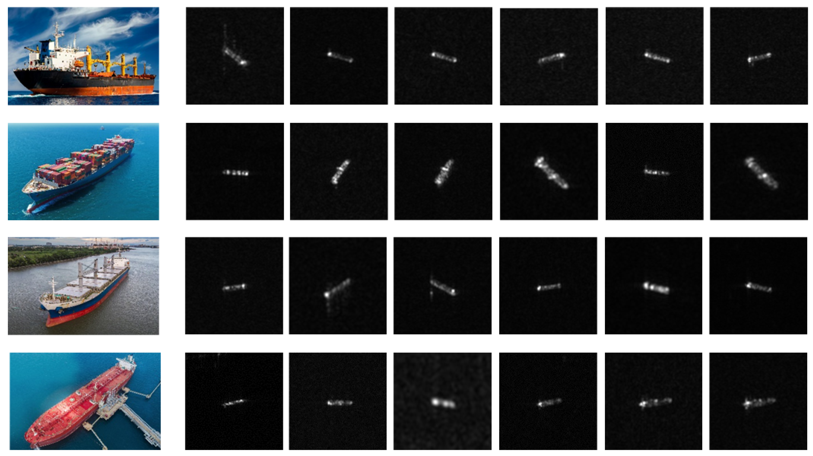
These previous methods have obtained remarkable performance for SAR ship classification tasks by training models with large-scale datasets. However, despite the great quantity of SAR images, the volume of available SAR ship classification data is relatively small, especially for some maritime military targets such as destroyers and aircraft carriers, while the manual labeling cost is expensive. DL-based models trained on small-scale datasets usually suffer from the overfitting problem, thus reducing the generalization ability. Furthermore, different from optical images, the information on SAR images is limited because of the shortcoming of the SAR imaging mechanism. Some examples are shown in Figure 1 where we can see that the appearance of different types of ships has subtle differences, while the appearance of the same type of ship has distinct changes. This problem is called intraclass diversity and interclass similarity, and further degrades the classification performance.

To address these problems, this article proposes an LST-ACGAN for SAR ship classification by introducing an ACGAN [19] to generate new samples, assigning smooth labels [20] to generated samples, and integrating the triplet loss [21] into the ACGAN. An ACGAN is one of the GAN’s variants [19,22,23]. By adding category information to the generator and an auxiliary classifier to the discriminator, the ACGAN can generate samples with category labels and also has classification capacity. Due to the excellent characteristics of the ACGAN, this article introduces its architecture to alleviate the data insufficiency problem by generating ship samples with category labels while classifying ships. However, the training of an ACGAN typically requires plenty of data to learn the distribution of real images. Otherwise, it is hard to generate samples with precise categories and prone to model collapse during training. To address this problem, this article assigns smooth labels to generated samples rather than hard labels to prevent the model from being overconfident in generated images during training, and the CE loss is replaced with smooth label SL-CE loss for the classification of generated images. By assigning smooth labels, the training procedure is made more stable, and generated samples can also play the role of regularization.

Furthermore, in the SAR image dataset, targets belonging to the same class usually have high intraclass diversity, while targets belonging to different classes usually have high interclass similarity. To address this problem, triplet loss [21] is integrated into the ACGAN. Different from traditional CNNs with CE loss, the triplet loss can enhance the classification margin by pulling the intraclass samples closer and pushing the interclass samples farther in the embedding space. During training, triplets are built by sampling anchor images, positive images that belong to the same classes, and negative images that belong to other classes, and then the triplet loss is jointly optimized with the multi-task loss. By integrating these modules, the proposed method can learn better classification margins and obtain higher performance.

Our contribution can be summarized as follows:

(1)

An ACGAN is introduced to generate images for the small-scale SAR ship classification task to alleviate the overfitting problem. To prevent the model from mode collapse, smooth labels are assigned to generated images to avoid the model being overconfident in the generated images.

(2)

Triplet loss is integrated into the ACGAN to learn discriminative features by pulling the intraclass samples closer and pushing the interclass samples farther.

(3)

Extensive experiments in three aspects on the OpenSARShip [24] dataset demonstrate the superior performance of our method over the previous methods.

The article is organized into five sections. Section 2 introduces the ACGAN and triplet loss that are relevant to our method. Section 3 presents the proposed LST-ACGAN method in detail. Section 4 describes the experimental settings and results. Section 5 is the conclusion.

2. Related Works

This section introduces some preliminary knowledge of the ACGAN and triplet loss.

2.1. ACGAN

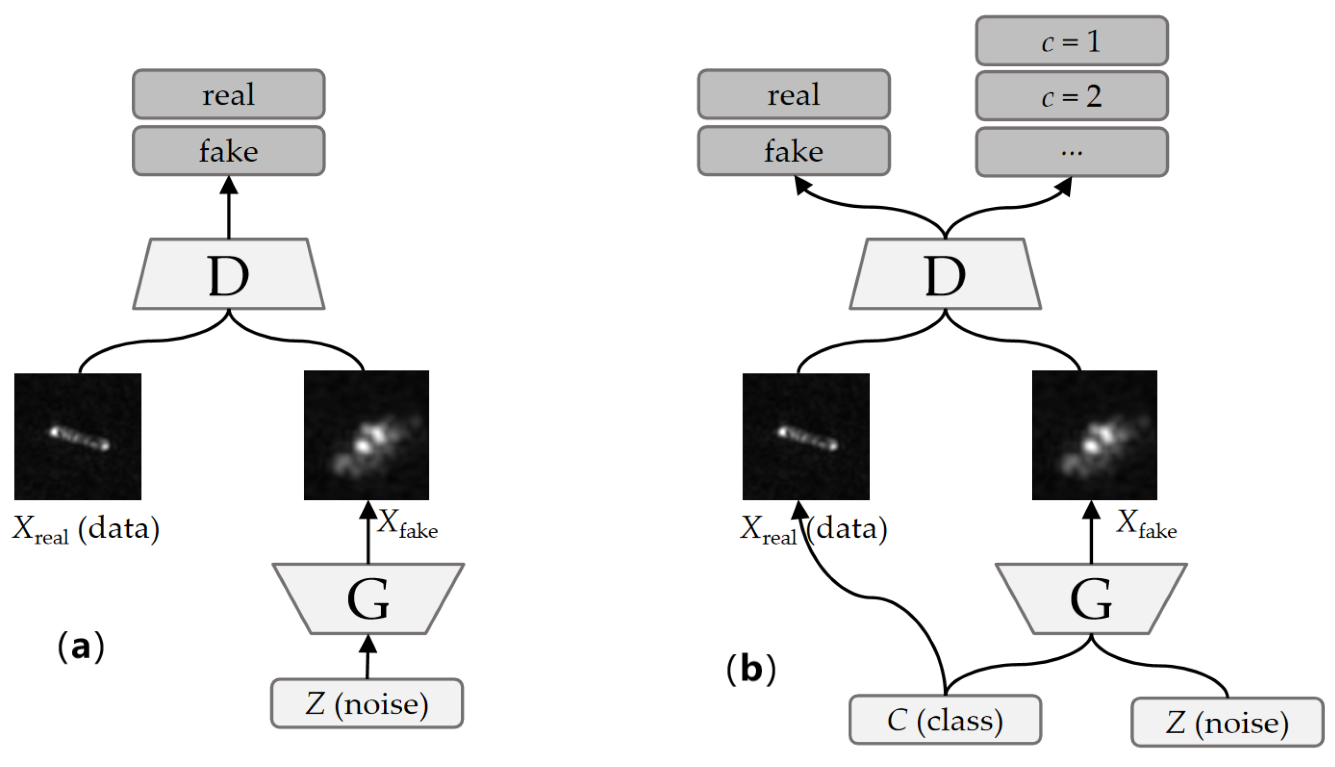
Different from the traditional GAN shown in Figure 2a, an ACGAN integrates category information into the input of the generator (G) for the generated images, and an auxiliary classification network to the discriminator (D). Figure 2b explains the network architecture of an ACGAN. The D aims to distinguish between real and generated images and classifies them. Its optimization objective can be represented as:

$$\begin{array}{cc}\hfill \underset{D}{max}V(D,G)& ={\mathrm{E}}_{x\sim p_{\mathrm{data}}\left(x\right)}[logD\left(x\right)]+{\mathrm{E}}_{z\sim p_z\left(z\right)}\left[log\left(1-D\left(G\left(z\mid y_{\mathrm{fake}}\right)\right)\right)\right]\hfill \\ \hfill & +{\mathrm{E}}_{x\sim p_{\mathrm{data}}\left(x\right)}[logp(y\mid x)]+{\mathrm{E}}_{z\sim p_z\left(z\right)}\left[logp\left(y_{\mathrm{fake}}\mid G\left(z\mid y_{\mathrm{fake}}\right)\right)\right]\hfill \end{array}$$

(1)

where $x\sim p_{\mathrm{data}}\left(x\right)$, y, and $z\sim p_z\left(z\right)$ represent the distribution of real images, the label of real images, and the distribution of noises, respectively. $y_{\mathrm{fake}}$ and $G\left(z\right|y_{\mathrm{fake}})$ represent the category label of the generated image and the generated image, respectively. $D\left(x\right)$ and $D\left(G\left(z\right|y_{\mathrm{fake}})\right)$ represent the correct and wrong discrimination probability of the D, respectively, and $p\left(y\right|x)$ and $p\left(y_{\mathrm{fake}}\right|G\left(z\right|y_{\mathrm{fake}}))$ represent the correct classification probability for real and generated images, respectively. The G is trained to generate more realistic images with category labels, and its optimization objective can be represented as:

$$\begin{array}{cc}\hfill \underset{G}{min}V(D,G)=& {\mathrm{E}}_{z\sim P_z\left(z\right)}\left[log\left(1-D\left(G\left(z\mid y_{\mathrm{fake}}\right)\right)\right]-\right.\hfill \\ \hfill & {\mathrm{E}}_{z\sim P_z\left(z\right)}\left[logp\left(y_{\mathrm{fake}}\mid G\left(z\mid y_{\mathrm{fake}}\right)\right)\right]\hfill \end{array}$$

(2)

The joint optimization objective of an ACGAN can be represented as:

$$\begin{array}{cc}\hfill \underset{G}{min}\underset{D}{max}V(D,G)& ={\mathrm{E}}_{x\sim p_{\mathrm{data}}}[logD\left(x\right)]+{\mathrm{E}}_{z\sim p_z\left(z\right)}[log(1-D\left(G(z\mid y)\right))]\hfill \\ \hfill & +{\mathrm{E}}_{x\sim p_{\mathrm{data}}}[logp(c\mid x)]\pm {\mathrm{E}}_{z\sim p_z\left(z\right)}[logp(c\mid G(z\mid y))]\hfill \end{array}$$

(3)

By the adversarial training procedure, the abilities of the G and D can be improved simultaneously and eventually balanced.

2.2. Triplet Loss

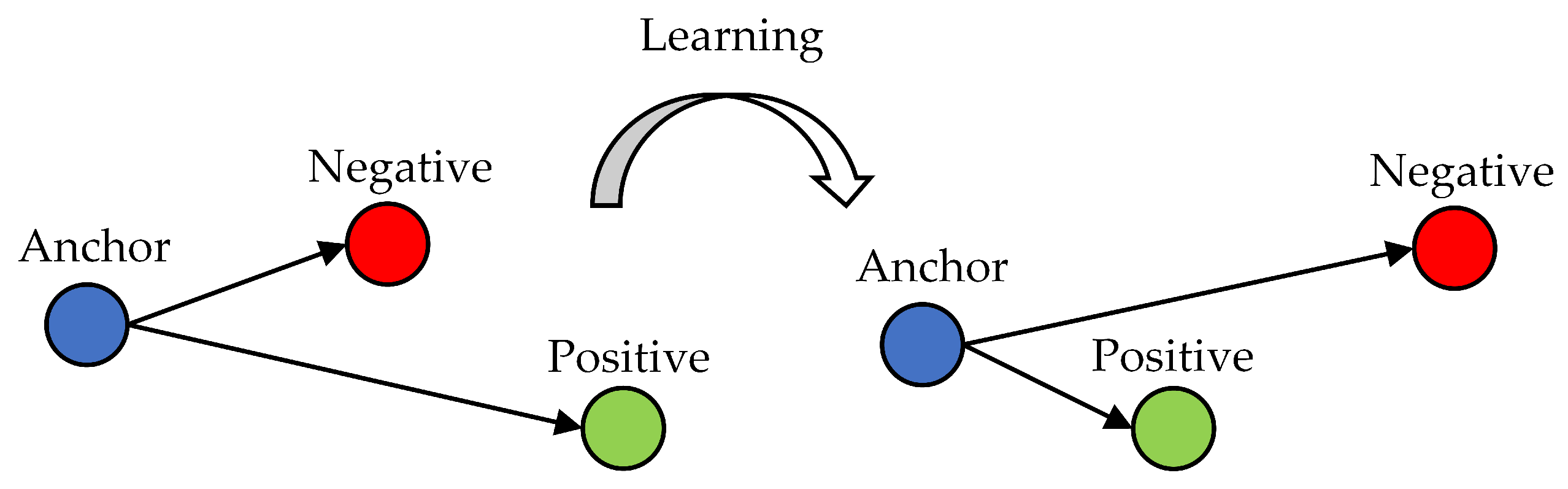
DML combines deep learning and distance metric learning to learn nonlinear features and similarities between data. Triplet loss and contrastive loss [25] have been commonly used in DML paradigms. Compared to contrastive loss, triplet loss can obtain better performance by pulling intraclass samples closer as well as pushing the interclass samples farther, and has been broadly applied in retrieval tasks [26,27]. The optimization process for triplet loss is shown in Figure 3, and the loss function can be represented as:

$$l_{\mathrm{triplet}}=max\left(d\left(f\left(x^a\right),f\left(x^p\right)\right)-d\left(f\left(x^a\right),f\left(x^n\right)\right)+\alpha ,0\right)$$

(4)

where $x^a$ represents the anchor image, and $x^p$ and $x^n$ represent the positive and negative image, respectively. $\alpha$ is a margin between positive and negative pairs, and $d($·) represents the distance function, usually the Euclidean distance. Statistically, by optimizing the triplet loss in Formula (4), the model can learn to close the distance between the anchor and the positive sample while pushing the distance between the anchor and the negative sample away. After training, the model can map the same class samples into one cluster and keep the distance between clusters larger than $\alpha$.

3. Proposed Method

This section firstly explains the overall structure of the LST-ACGAN method, secondly introduces the network architecture of the G and the D, thirdly explains label smoothing for generated images, then presents discriminative feature learning via triplet loss, and finally gives the multi-task learning loss function.

3.1. Overall Structure of LST-ACGAN

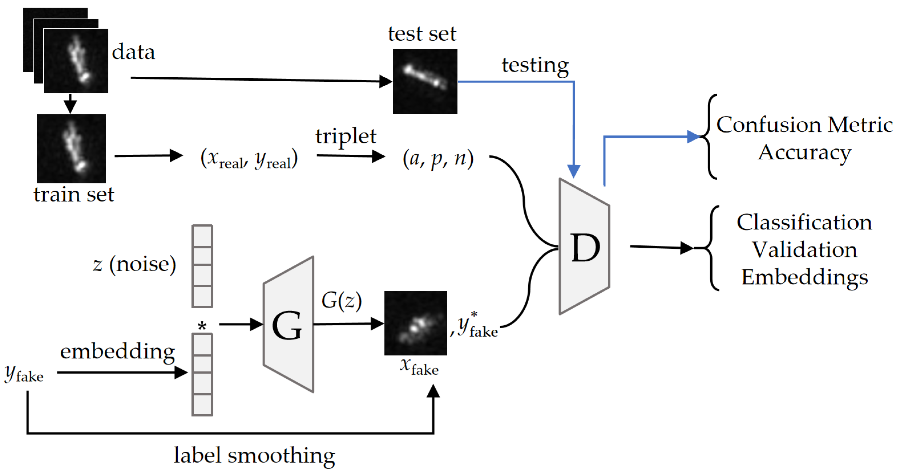
DL-based SAR ship classification has achieved remarkable performance with large-scale training samples. However, when the training data are insufficient, these methods can barely learn the distribution of data and are prone to overfitting. To address this issue, we present a GAN-based algorithm, named LST-ACGAN, to generate images and classify samples simultaneously. As shown in Figure 4, the overall model of the LST-ACGAN includes a generator G and a discriminator D. The G can generate images with category labels, while the discriminator can validate whether an input image is real and, meanwhile, classify it. Moreover, smooth labels are assigned to generated images and SL-CE loss is proposed as classification loss for generated images to avoid model collapse as well as regularize the model during training. Furthermore, triplet loss is integrated into the network to learn discriminative deep features. During training, triplets are built by sampling anchor, positive, and negative images from real images, and fed into the discriminator together with generated images. Multi-task learning losses are jointly optimized for classification, validation, and discriminative deep feature embeddings.

3.2. Network Architecture

3.2.1. The Generator

As shown in Figure 4, for a given noise vector z and label $y_{\mathrm{fake}}$, the LST-ACGAN first embeds $y_{\mathrm{fake}}$, and assigns category information to z by element-wise multiplying z and embedded $y_{\mathrm{fake}}$:

$$z^{\prime }=\mathrm{embedding}\left(y_{\mathrm{fake}}\right)\circ z$$

(5)

where embedding(·) represents the embedding layer, which embeds label $y_{\mathrm{fake}}$ to the latent space; ∘ represents element-wise multiplication. Thus, the category information is fully fused with the noise vector. Then, taking $z^{\prime }$ as the input, the generator generates images via DCNNs. The generator includes a transformation layer, 2 UC layers, and a generation layer (see

Table 1. Network architecture of the generator. There are five stages in this network. Specifically, for the convolution layer, the parameters c, k, s, and p represent the channel size, kernel size, stride, and padding size, respectively. For the leaky ReLU layer, $\alpha$ represents the negative slope. The generated image is resized to 1 × H × W, and is set to 1 × 64 × 64 in this article.

Stage	Layers	Settings	Outputs
Transformation	FC	$128\times \mathrm{H}/4\times \mathrm{W}/4$	$128\times \mathrm{H}/4\times \mathrm{W}/4$
	Reshape	$(128,\mathrm{H}/4,\mathrm{W}/4)$	$128\times \mathrm{H}/4\times \mathrm{W}/4$
	$\mathrm{BN}$	-	$128\times \mathrm{H}/4\times \mathrm{W}/4$
UC1	Upsampling	$2\times$	$128\times \mathrm{H}/2\times \mathrm{W}/2$
	Convolution	$\mathrm{c}=128,\mathrm{k}=3,\mathrm{s}=1,\mathrm{p}=1$	$128\times \mathrm{H}/2\times \mathrm{W}/2$
	$\mathrm{BN}$	-	$128\times \mathrm{H}/2\times \mathrm{W}/2$
	Leaky ReLU	$\alpha =0.2$	$128\times \mathrm{H}/2\times \mathrm{W}/2$
UC2	Upsampling	$2\times$	$128\times \mathrm{H}\times \mathrm{W}$
	Convolution	$\mathrm{c}=64,\mathrm{k}=3,\mathrm{s}=1,\mathrm{p}=1$	$64\times \mathrm{H}\times \mathrm{W}$
	BN	-	$64\times \mathrm{H}\times \mathrm{W}$
	Leaky ReLU	$\alpha =0.2$	$64\times \mathrm{H}\times \mathrm{W}$
Generation	Convolution	$\mathrm{c}=1,\mathrm{k}=3,\mathrm{s}=1,\mathrm{p}=1$	$1\times \mathrm{H}\times \mathrm{W}$
	Tanh	-	$1\times \mathrm{H}\times \mathrm{W}$

). For the input vector $z^{\prime }$, the transformation layer transforms it from a one-dimensional vector to a three-dimensional feature map by a fully connected (FC) layer, reshape operation layer, and batch normalization (BN) [28] layer. Then, the UC layer, taking UC1 as an example, upsamples the input feature map by upsampling the operation followed by a convolution layer, a BN layer, and a Leaky ReLU layer [29]. Finally, the generation layer reduces the channels of the feature map via a 3 × 3 convolution layer with a channel size of one, and constrains the output into (−1, 1) by the tanh function.

3.2.2. Discriminator

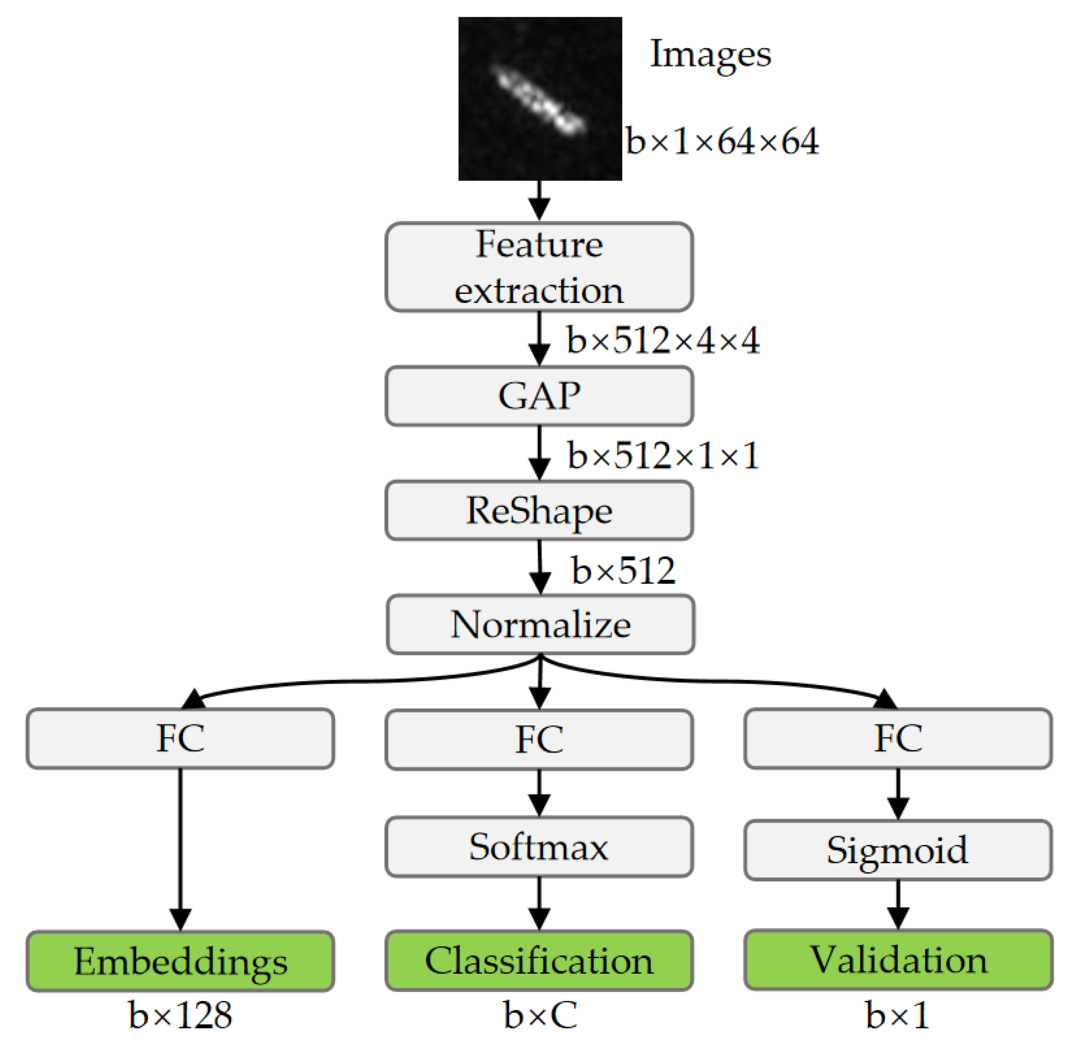
The discriminator of the LST-ACGAN adopts a multi-task learning architecture for classification, validation, and deep feature embedding learning. The network architecture of the discriminator is shown in Figure 5. The discriminator mainly includes the feature extraction network and three multi-task learning subnetworks. In this article, the pretrained ResNet18 [30] with the FC layer removed is adopted as the feature extraction network. For input images, deep feature maps are extracted by the feature extraction network and converted into vectors by the global average pooling (GAP) and reshape operations. Then, the vectors are normalized with L2 normalization to stabilize the learning process. Finally, the discriminator outputs the embeddings, classification results, and validation results by the embedding subnetwork, classification subnetwork, and validation subnetwork, respectively. Specifically, the classification subnetwork classifies the input image via the softmax function:

$$q_i=\frac{exp\left(p_i\right)}{{\sum }_{j=1}^{C}exp\left(p_j\right)}$$

(6)

where C represents the number of categories, $p_i$, (i = 1, 2, …, C) represents the classification vector, and $q_i$ represents the probability that the image belongs to the i-th category. For the validation subnetwork, the outputs are constrained to (0, 1) by the sigmoid activation function:

$$p\left(v\right)=\frac{1}{1+exp(-v))}$$

(7)

where v represents the binary classification vector, and $p\left(v\right)$ represents the probability that the input image belongs to the real class.

3.3. Label Smoothing for Generated Images

In the multi-class classification task, the input image is usually assigned hard labels, which can be represented as:

$$y_i=\left\{\begin{array}{cc}1& i=\mathrm{true}\\ 0& \mathrm{otherwise}\end{array}\right.$$

(8)

where $y_i$ (i = 1, 2, …, C) represents a one-hot vector, $y_i$ = 1, when the image belongs to the to i-th category. The classification network outputs the probability that the input image belongs to each category via the softmax function, and the CE loss serves as the classification loss:

$$\begin{array}{cc}\hfill l_{\mathrm{CE}}& =-\sum _{i=1}^C{y}_{i}log{q}_i\hfill \\ \hfill & =-log{q}_{\mathrm{true}}\hfill \end{array}$$

(9)

Generally, the generated images of a GAN are not perfect, especially for an ACGAN with category labels. When the training data are insufficient, it is more difficult for an ACGAN to generate images with accurate category labels. However, a hard label with CE loss encourages the model to output predicted labels equal to 1 or 0 for target or nontarget categories. In the logit classification vector, the value of the target category $p_i$ will tend to infinity, making the model too confident for its prediction. Thus, generated images by an ACGAN with the hard labels are prone to model collapse during training if the training samples are insufficient. To address this problem, we assign smooth labels to the generated images rather than hard labels, which can be represented as:

$$y_i^{*}=\left\{\begin{array}{cc}1-\epsilon & i=\mathrm{true}\\ \frac{\epsilon }{N-1}& \mathrm{otherwise}\end{array}\right.$$

(10)

where $\epsilon$ is a hyperparameter. The classification loss for generated images is replaced by SL-CE loss, which can be represented as:

$$\begin{array}{cc}\hfill l_{\mathrm{LS}-\mathrm{CE}}& =-\sum _{i=1}^N{y}_i^{*}log{q}_i\hfill \\ \hfill & =-\left[(1-\epsilon )log{q}_{\mathrm{true}}+\frac{\epsilon }{N-1}\sum _{i\ne \mathrm{true}}log{q}_i\right]\hfill \end{array}$$

(11)

In this way, by adding noise to the generated image, this avoids the model over-confidence in the target category, making the prediction difference between the target category and the nontarget category not so large, thus avoiding model collapse during training and, meanwhile, regularizing the model.

3.4. Discriminative Feature Learning via Triplet Loss

The triplet loss is integrated into the ACGAN for discriminative deep feature learning to address the high intraclass diversity and interclass similarity issues. The key ideas of triplet loss are mentioned in Section 2.2; in this section, we explain the integration of triplet loss in detail.

As mentioned in Section 3.3, we assign smooth labels to generated images since the generator cannot generate images with precise category labels. The triplet loss, which aims to learn discriminative deep features by pulling the intraclass samples closer and pushing the interclass samples farther, conflicts with the label smoothing for generated images. Therefore, triplet loss is only performed on real images. Specifically, selecting appropriate triplets is important for training the network. There are two triplet sampling paradigms: offline and online. Since the offline methods are not efficient for sampling triplets across the whole dataset, we adopt the online method following [21]. All the triplets that violate the following distance constraint in the embedding space are selected:

$$d\left(f\left(x^a\right),f\left(x^p\right)\right)+\alpha <d\left(f\left(x^a\right),f\left(x^n\right)\right)$$

(12)

where $d(·)$ represents the Euclidean distance; the margin $\alpha$ is set to 0.2 for all experiments.

3.5. Multi-Task Learning Loss Function

The generator G and discriminator D networks are alternately optimized during the training phase. Based on the validation results and classification results of the discriminator, the generator is optimized by the validation loss and classification loss. Specifically, the binary cross-entropy (BCE) loss is employed as the validation loss, which can be represented as:

$$l_{BCE}=-\left(y_v{}^{*}log\left(p\left(v\right)\right)+{\left(1-y_v\right)}^{*}log(1-p\left(v\right))\right)$$

(13)

where $y_v$ represents the binary label. The classification loss of the generator is SL-CE loss, and the total loss of the generator is formulated as follows:

$$L_{\mathrm{G}}={\lambda }_1{l}_{\mathrm{BCE}}\left(x_{\mathrm{fake}},1\right)+{\lambda }_2{l}_{\mathrm{LS}-\mathrm{CE}}\left(x_{\mathrm{fake}},y_{\mathrm{fake}}^{*}\right)$$

(14)

where $x_{\mathrm{fake}}$ and $y_{\mathrm{fake}}$ represent the generated image and the smooth label of the generated image, respectively, “1” represents the validation label of the generated image, and ${\lambda }_1$ and ${\lambda }_2$ represent the trade-off parameters. The discriminator aims to distinguish between real and generated images, classify them, and learn the deep feature embedding of real images and is optimized by the validation loss, classification loss, and triplet loss. Specifically, the discriminator assigns 0 and 1 to the generated image and real image for validation, and the BCE loss serves as the validation loss. The CE loss is used as the classification loss for real images, while the SL-CE loss is used for generated images. The overall loss of the D is formulated as follows:

$$\begin{array}{cc}\hfill L_D& ={\lambda }_3{l}_{\mathrm{BCE}}\left(x_{\mathrm{real}},1\right)+{\lambda }_4{l}_{\mathrm{BCE}}\left(x_{\mathrm{fake}},0\right)+{\lambda }_5{l}_{\mathrm{LS}-\mathrm{CE}}\left(x_{\mathrm{fake}},y_{\mathrm{fake}}^{*}\right)\hfill \\ \hfill & +{\lambda }_6{l}_{\mathrm{CE}}\left(x_{\mathrm{real}},y_{\mathrm{real}}\right)+{\lambda }_7{l}_{\mathrm{triplets}}\left(x^a,x^p,x^n\right)\hfill \end{array}$$

(15)

where $y_{\mathrm{real}}$ represents the hard label for the real image, and ${\lambda }_i$ (i = 3, 4, …, 7) represent the trade-off parameters. In this article, ${\lambda }_i$ (i = 1, 2, …, 7) are set to 1 by default for all experiments.

4. Experimental Settings and Result Analysis

In this part, we first introduce the dataset and training settings, then analyze the stability of the LST-ACGAN algorithm with different parameter settings, and then conduct the ablation study to analyze the performance of different loss function combinations. After that, we visualize and analyze the generated images of the LST-ACGAN, and finally, we compare with previous methods to demonstrate the effectiveness of the LST-ACGAN.

4.1. Datasets

The OpenSARShip [24] dataset was established for the Sentinel-1 ship classification task. It includes two product types: single look complex (SLC) and ground range detected (GRD). Considering that bulk carriers, container ships, and tankers cover around 80% of the international shipping market [6,31], in this paper, we obtained five common merchant vessels, including a bulk carrier, a cargo ship, a container ship, a general cargo ship, and a tanker from the open data sharing platform of OpenSARShip (https://Opensar.Sjtu.Edu.Cn/Project.html) (accessed on 9 July 2023) (see

Table 2. Number of each ship type.

Ship Type	Number
Bulk Carrier	1624
Cargo	2228
Container Ship	426
General Cargo	236
Tanker	352

).

As shown in

Table 3. Reconstructed subdatasets from OpenSARShip.

Ship Type	D1	D2	$\mathbf{T}$
Bulk Carrier	252	136	100
Cargo	-	136	100
Container Ship	252	136	100
General Cargo		136	100
Tanker	252	136	100

, based on these ship types, we reconstructed two subdatasets. First, 100 samples for each ship type were randomly selected as standard testing set T. Then, according to the class with the least number of samples, we reconstructed a class-balanced three-class training set D1 and a class-balanced five-class training set D2.

4.2. Training Details

A computer with the Intel i7-8700 CPU and NVIDIA GTX1080Ti GPU was utilized to conduct all experiments, and all codes were implemented by PyTorch. The structures of the model are shown in Table 1 and Figure 5.

To ensure the fairness of comparison, for all experiments, input images were resized to 64 × 64 pixels. Adam [32] was used as the optimizer with the learning rate set to 0.0002. The training batch size m was set to 128, and the total training epoch was 200. In each epoch, the samples were first reordered randomly, then input into the model batch-by-batch. The training procedure of the proposed model is shown in Algorithm 1. Specifically, none of the experiments in this article adopted any data augmentation methods.

Algorithm 1 Training procedure of the proposed algorithm.

Initialize the models G and D, number of epochs(nb_epoch = 200), batch_size m = 128

for epoch = 1:nb_epoch

for i = 1:nb_batch

Sample m vector randomly, calculate smoothing labels and generate corresponding fake images by G;

Sample m real images and randomly mix them with fake images;

Input mixed samples into the D, calculate the validation and classification losses, then update the weights of D and G;

Combine triplet samples and calculate the triplet loss, update the weights of D and G;

end

end

Obtain model D;

Input a testing sample into D, and obtain the prediction class.

The overall accuracy (OA) and confusion matrix (CM) are adopted as the evaluation indices. The OA indicates the whole classification accuracy and is defined as:

$$\mathrm{OA}=\frac{tp+tn}{tp+tn+fp+fn}\times 100\%$$

(16)

where $tp$, $tn$, $fn$, and $tn$ represent the true positives, false positives, false negatives, and true negatives, respectively. CM is the matrix in which the diagonal elements are the classification accuracy for each ship type.

4.3. Stability Analysis

The sensitivity analyses on the parameter $\epsilon$ in (10) and the embedding length are shown as follows.

4.3.1. Label Smoothing Parameter

To explore the effectiveness of the label smoothing, we conducted experiments on D1 with different $\epsilon$ selected from the set of {0.1, 0.2, 0.3, 0.4, 0.5, 0.6}. As shown in

Table 4. OA (%) on D1 using different label smoothing parameters.

ε	0.1	0.2	0.3	0.4	0.5	0.6
$\mathrm{OA}$	84.33	84.67	84.67	88.33	86.33	87.00

, we can observe that the performance is relatively stable with different $\epsilon$. The best performance is 88.33% with setting $\epsilon$ = 0.4. Therefore, $\epsilon$ was fixed to 0.4 for all of the following experiments.

4.3.2. Embedding Dimensionality

The dimensional value of the embedding was set to 64, 128, 256, and 512, respectively. From

Table 5. OA (%) on D1 with different embedding lengths.

Dim.	64	128	256	512
OA	85.66	$\mathbf{88.33}$	84.66	85.33

, we can observe that the accuracy drops if the embedding dimensionality is too small or too large. This might be because the representational ability is weak if the embedding is small, while the model will overfit to the limited data if the embedding is too large. Thus, all the embedding lengths were fixed to 128 for the following experiments.

4.4. Ablation Study

The ablation study results with different loss function combinations are shown in

Table 6. OA (%) on D1 with different loss combinations.

Objective Function Combinations	OA
CE loss	75.33
CE loss + Triplet loss	85.66
SL-CE loss	83.33
SL-CE loss + Triplet loss	88.33

, where “CE loss” and “SL-CE loss” represent the classification loss for generated images with hard label and smooth labels, respectively, and “Triplet loss” represents the loss for deep feature embedding learning. We can observe that compared with the baseline network optimized by CE loss, the integration of SL-CE loss and triplet loss obtains better results. Specifically, the “SL-CE loss + Triplet loss” combination obtains the best performance of 88.33%, which is 13% higher than the baseline (75.33%). Therefore, the integration of the smooth label and the triplet loss is crucial for better ship classification performance.

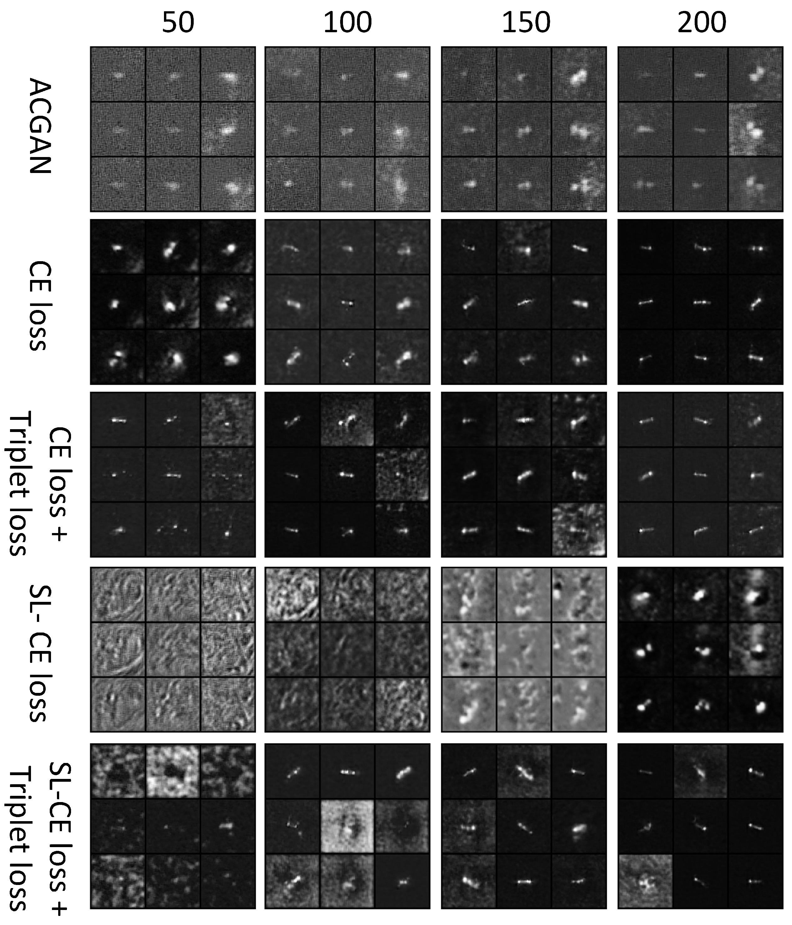
4.5. Visualization of Generated Images

The generated images are shown in Figure 6. Each row represents a method with a different loss function, while each column represents the result after training 50, 100, 150, and 200 epochs. We can observe that, generally, the quality of our method is better than the ACGAN (first row). Visually, the LST-ACGAN with CE loss (second row) obtains the optimal quality generated images; this might be because the CE loss forces the model to generate images that certainly belong to given classes. However, generated high-quality images do not necessarily mean better classification results because these samples are difficult to extend to the distribution of original samples and have a larger distance to the classification margin, making them less useful for improving the classification performance. The image quality of SL-CE loss + triplet loss is better than only using SL-CE loss; this might be because the triplet loss can force the model to generate images that have a closer distance to the given class.

4.6. Extensive Comparisons

The proposed method was also compared with previous DCNN methods, including the ACGAN [19], ResNet18 [30], and DenseNet121 [33], to demonstrate its effectiveness.

4.6.1. Three-Class Classification Task

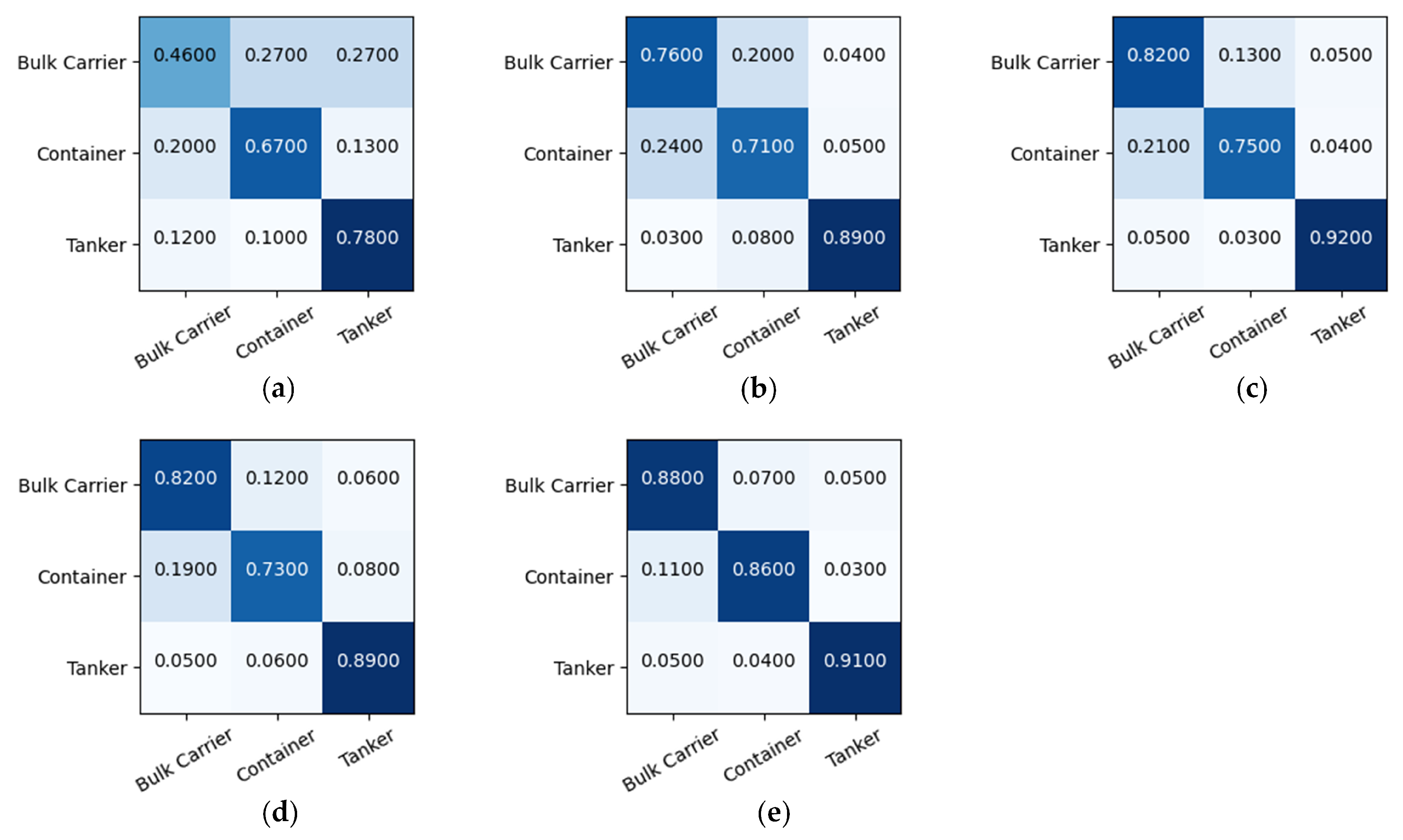
The three-class classification results of different models are shown in

Table 7. OA (%) on D1 using different network architectures.

Network	OA
ACGAN	63.67
ResNet18	78.67
DenseNet121	83.00
Xception	81.33
LST-ACGAN	88.33
LST-ACGAN + DenseNet121	87.33
LST-ACGAN + Xception	84.00

. The proposed LST-ACGAN obtains the best OA of 88.33%, which is 24.66% high than the ACGAN (63.67%), 9.66% higher than ResNet18 (78.67%), 5.33% higher than DenseNet121 (83.00%), and 7% higher than Xception (81.33%). Furthermore, by combining the proposed method with DenseNet121 and Xception, there are improvements of 4.33% and 2.67%, respectively, compared to the original OA.

The CMs of different models are shown in Figure 7. We can observe that compared to the ACGAN, ResNet, DenseNet121, and Xception obtain higher performances, showing that the complex models can learn more discriminative features. The classification accuracy of the LST-ACGAN on these three ship types is better than most of the previous methods. In particular, the proposed method is 6% higher than DenseNet121 and Xception in the Bulk Carrier class, and 11% higher than DenseNet121 in the Container class. This result shows that by adding the triplet loss and label smoothing methods, the proposed method can extract more discriminative deep features.

4.6.2. Five-Class Classification Task

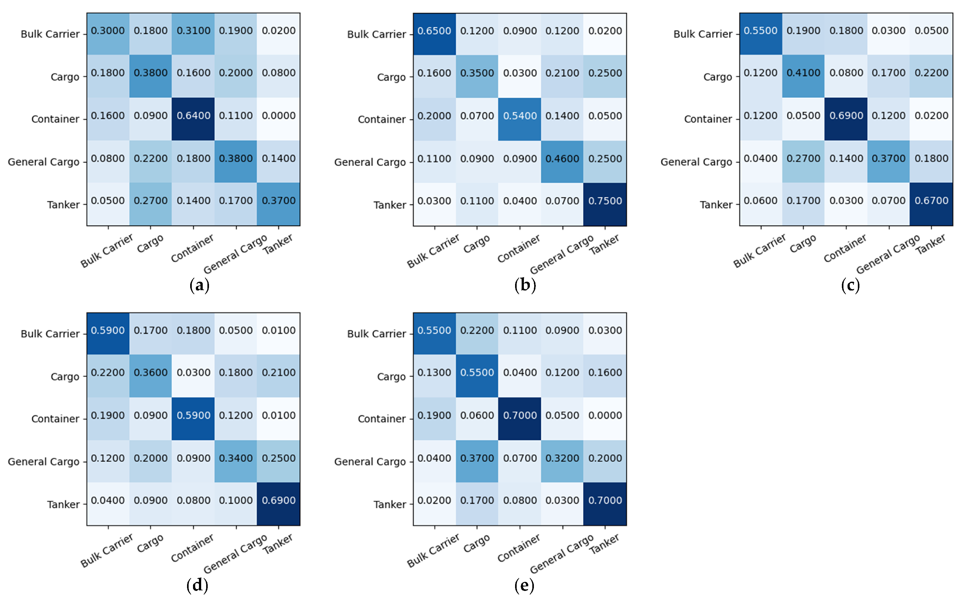
The five-class classification results of different models are shown in

Table 8. OA (%) on D2 using different network architectures.

Network	OA
ACGAN	41.40
ResNet18	54.00
DenseNet121	53.80
Xception	51.40
LST-ACGAN	56.40
LST-ACGAN + DenseNet121	54.60
LST-ACGAN + Xception	52.00

. The proposed LST-ACGAN obtains the best OA of 56.40%, which is 15% high than the ACGAN 41.40%), 2.4% higher than ResNet18 (54.00%), 5.1% higher than DenseNet121 (51.30%), and 6.32% higher than Xception (50.08%). Furthermore, by combining the proposed method with DenseNet121 and Xception, there are improvements of 0.8% and 0.6%, respectively, compared to the original OA.

The CMs of different models are shown in Figure 8. We find that the ship types of Cargo and General Cargo are difficult to distinguish due to their apparent similarity; thus, the classification accuracies of these two classes’ samples are relatively low. The accuracy of our method on the Cargo class is the highest among all methods, while the accuracy of the General Cargo class is relatively low. This might be because the features of the General Cargo class are more complex and have varied distribution compared to the Cargo class, making it hard for the model to distinguish them. Moreover, the classification accuracy of the LST-ACGAN on these five ship types is better than the majority of previous methods.

5. Conclusions

This article proposes a GAN-based method for the SAR ship classification task. The proposed method explores a novel way for small-scale sample classification of SAR images. By combining and jointly optimizing the data generation and classification modules, the proposed model can generate new samples to improve the generalization ability as well as classify samples into corresponding classes. By incorporating the label smoothing method and triplet loss, the model can learn more distinguishable features for different class samples. Experiments on the three- and five-class classification tasks demonstrate that the proposed LST-ACGAN method performs better than the compared models.

References

- Martino, G.D.; Iodice, A.; Riccio, D.; Ruello, G. Ocean monitoring with SAR: An overview. In Proceedings of the IEEE OCEANS, Genova, Italy, 18–21 May 2015; p. 48. [Google Scholar]
- Margarit, G.; Tabasco, A. Ship Classification in Single-Pol SAR Images Based on Fuzzy Logic. IEEE Trans. Geosci. Remote Sens. 2011, 49, 3129–3138. [Google Scholar] [CrossRef]
- Ji, K.; Xing, X.; Chen, W.; Zou, H.; Chen, J. Ship classification in TerraSAR-X SAR images based on classifier combination. In Proceedings of the IEEE International Geoscience and Remote Sensing Symposium, Melbourne, VIC, Australia, 21–26 July 2013. [Google Scholar]
- Lang, H.; Jie, Z.; Xi, Z.; Meng, J. Ship Classification in SAR Image by Joint Feature and Classifier Selection. IEEE Geosci. Remote Sens. Lett. 2015, 13, 212–216. [Google Scholar] [CrossRef]
- Lang, H.; Wu, S. Ship Classification in Moderate-Resolution SAR Image by Naive Geometric Features-Combined Multiple Kernel Learning. IEEE Geosci. Remote Sens. Lett. 2017, 14, 1765–1769. [Google Scholar] [CrossRef]
- Jiang, M.; Yang, X.; Dong, Z.; Shuai, F.; Meng, J. Ship Classification Based on Superstructure Scattering Features in SAR Images. IEEE Geosci. Remote Sens. Lett. 2016, 13, 616–620. [Google Scholar] [CrossRef]
- Zhu, J.; Qiu, X.; Pan, Z.; Zhang, Y.; Lei, B. An Improved Shape Contexts Based Ship Classification in SAR Images. Remote Sens. 2017, 9, 145. [Google Scholar] [CrossRef]
- Lin, H.; Song, S.; Jian, Y. Ship Classification Based on MSHOG Feature and Task-Driven Dictionary Learning with Structured Incoherent Constraints in SAR Images. Remote Sens. 2018, 10, 190. [Google Scholar] [CrossRef]
- He, J.; Wang, Y.; Liu, H. Ship Classification in Medium-Resolution SAR Images via Densely Connected Triplet CNNs Integrating Fisher Discrimination Regularized Metric Learning. IEEE Trans. Geosci. Remote Sens. 2020, 59, 3022–3039. [Google Scholar] [CrossRef]
- Zhang, T.; Zhang, X. A polarization fusion network with geometric feature embedding for SAR ship classification. Pattern Recognit. 2022, 123, 108365. [Google Scholar] [CrossRef]
- Li, J.; Qu, C.; Peng, S. Ship classification for unbalanced SAR dataset based on convolutional neural network. J. Appl. Remote Sens. 2018, 12, 1–13. [Google Scholar] [CrossRef]
- Dechesne, C.; Lefèvre, S.; Vadaine, R.; Hajduch, G.; Fablet, R. Ship Identification and Characterization in Sentinel-1 SAR Images with Multi-Task Deep Learning. Remote Sens. 2019, 11, 2997. [Google Scholar] [CrossRef]
- Firoozy, N.; Sandirasegaram, N. Tackling SAR Imagery Ship Classification Imbalance via Deep Convolutional Generative Adversarial Network. Can. J. Remote Sens. 2021, 47, 295–308. [Google Scholar] [CrossRef]
- Zhang, Y.; Guo, X.; Leung, H.; Li, L. Cross-task and cross-domain SAR target recognition: A meta-transfer learning approach. Pattern Recognit. 2023, 138, 109402. [Google Scholar] [CrossRef]
- Zhao, Z.; Jiao, L.; Zhao, J.; Gu, J.; Zhao, J. Discriminant deep belief network for high-resolution SAR image classification. Pattern Recognit. 2017, 61, 686–701. [Google Scholar] [CrossRef]
- Zeng, L.; Zhu, Q.; Lu, D.; Zhang, T.; Yang, J. Dual-polarized SAR Ship Grained Classification Based on CNN with Hybrid Channel Feature Loss. IEEE Geosci. Remote Sens. Lett. 2021, 19, 1–5. [Google Scholar] [CrossRef]
- Zhang, Y.; Lei, Z.; Yu, H.; Zhuang, L. Imbalanced High-Resolution SAR Ship Recognition Method Based on a Lightweight CNN. IEEE Geosci. Remote Sens. Lett. 2022, 19, 1–5. [Google Scholar] [CrossRef]
- Dong, G.; Liu, H. A hierarchical receptive network oriented to target recognition in SAR images. Pattern Recognit. 2022, 126, 108558. [Google Scholar] [CrossRef]
- Shlens, A.O.O. Conditional Image Synthesis With Auxiliary Classifier GANs. In Proceedings of the Computer Vision and Pattern Recognition, Sydney, Australia, 6–11 August 2016. [Google Scholar]
- Szegedy, C.; Vanhoucke, V.; Ioffe, S.; Shlens, J.; Wojna, Z. Rethinking the Inception Architecture for Computer Vision. In Proceedings of the IEEE Conference on Computer Vision and Pattern Recognition (CVPR), Las Vegas, NV, USA, 26 June–1 July 2016; pp. 2818–2826. [Google Scholar]
- Schroff, F.; Kalenichenko, D.; Philbin, J. FaceNet: A unified embedding for face recognition and clustering. In Proceedings of the IEEE Conference on Computer Vision and Pattern Recognition, CVPR 2015, Boston, MA, USA, 7–12 June 2015; IEEE Computer Society: Washington, DC, USA, 2015; pp. 815–823. [Google Scholar] [CrossRef]
- Goodfellow, I.J.; Pouget-Abadie, J.; Mirza, M.; Xu, B.; Warde-Farley, D.; Ozair, S.; Courville, A.; Bengio, Y. Generative Adversarial Networks. Adv. Neural Inf. Process. Syst. 2014, 3, 2672–2680. [Google Scholar] [CrossRef]
- Arjovsky, M.; Chintala, S.; Bottou, O. Wasserstein generative adversarial networks. In Proceedings of the International Conference on Machine Learning, Sydney, Australia, 6–11 August 2017. [Google Scholar]
- Huang, L.; Liu, B.; Li, B.; Guo, W.; Yu, W.; Zhang, Z.; Yu, W. OpenSARShip: A Dataset Dedicated to Sentinel-1 Ship Interpretation. IEEE J. Sel. Top. Appl. Earth Obs. Remote Sens. 2017, 11, 195–208. [Google Scholar] [CrossRef]
- Chopra, S.; Hadsell, R.; Lecun, Y. Learning a similarity metric discriminatively, with application to face verification. In Proceedings of the 2005 IEEE Computer Society Conference on Computer Vision and Pattern Recognition, San Diego, CA, USA, 20–25 June 2005. [Google Scholar]
- Warburg, F.; Jørgensen, M.; Civera, J.; Hauberg, S. Bayesian Triplet Loss: Uncertainty Quantification in Image Retrieval. In Proceedings of the 2021 IEEE/CVF International Conference on Computer Vision, ICCV 2021, Montreal, QC, Canada, 10–17 October 2021; IEEE: New York, NY, USA, 2021; pp. 12138–12148. [Google Scholar] [CrossRef]
- Zhang, M.; Cheng, Q.; Luo, F.; Ye, L. A Triplet Non-Local Neural Network with Dual-Anchor Triplet Loss for High Resolution Remote Sensing Image Retrieval. IEEE J. Sel. Top. Appl. Earth Obs. Remote Sens. 2021, 14, 2711–2723. [Google Scholar] [CrossRef]
- Ioffe, S.; Szegedy, C. Batch Normalization: Accelerating Deep Network Training by Reducing Internal Covariate Shift. In Proceedings of the 32nd International Conference on Machine Learning, ICML, Lille, France, 6–11 July 2015; Volume 37, pp. 448–456. [Google Scholar]
- Maas, A.; Hannun, A.; Ng, A. Rectifier Nonlinearities Improve Neural Network Acoustic Models. In Proceedings of the ICML Work. Deep Learn. Audio, Speech Lang, Atlanta, GA, USA, 17–19 June 2013. [Google Scholar]
- He, K.; Zhang, X.; Ren, S.; Sun, J. Deep Residual Learning for Image Recognition. In Proceedings of the 2016 IEEE Conference on Computer Vision and Pattern Recognition (CVPR), Las Vegas, NV, USA, 27–30 June 2016. [Google Scholar]
- Zhang, X. Injection of Traditional Hand-Crafted Features into Modern CNN-Based Models for SAR Ship Classification: What, Why, Where, and How. Remote Sens. 2021, 13, 2091. [Google Scholar] [CrossRef]
- Kingma, D.P.; Ba, J. Adam: A Method for Stochastic Optimization. In Proceedings of the 3rd International Conference on Learning Representations, ICLR, San Diego, CA, USA, 7–9 May 2015. [Google Scholar]
- Iandola, F.N.; Moskewicz, M.W.; Karayev, S.; Girshick, R.B.; Darrell, T.; Keutzer, K. DenseNet: Implementing Efficient ConvNet Descriptor Pyramids. arXiv 2014, arXiv:1404.1869. [Google Scholar]
Figure 1.
Optical images and corresponding SAR of cargo ship (first line), container ship (second line), bulk carrier (third line), and tanker (fourth line).
Figure 2.
Network architecture of GAN and ACGAN. (a) GAN; (b) ACGAN.
Figure 3.
Triplet loss optimization process. Triplet loss aims at minimizing the distance between the anchor (blue) and a positive (green) sample that have the same class labels, and maximizing the distance between the anchor and a negative (red) sample that have different class labels.
Figure 4.
Overall structure of the LST-ACGAN. The blue line represents the testing phase and only utilizes the D to obtain the confusion metric.
Figure 5.
Network details of the discriminator. The discriminator mainly consists of the feature extraction network and three multi-task learning subnetworks, which are optimized with the triplet loss, multi-class classification loss, and binary-class classification loss, respectively. Symbols b, N, and C represent the batch size, embedding size, and the number of categories, respectively.
Figure 6.
Generated images when training after 50, 100, 150, 200 epochs of LST-ACGAN with different losses in the ablation study.
Figure 7.
Confusion metrics of different network architectures for three-class classification tasks. (a) ACGAN; (b) ResNet18; (c) DenseNet121; (d) Xception; (e) LST-ACGAN.
Figure 8.
Confusion metrics of different network architectures for five-class classification tasks. (a) ACGAN; (b) ResNet18; (c) DenseNet121; (d) Xception; (e) LST-ACGAN.