
Unusual Enhancement of the Optical Depth on the Continental Shelf Depth Latitudinal Variation in the Stratospheric Polar Vortex


Abstract
:1. Introduction
2. Materials and Methods
2.1. DOAS
2.2. Reconstructing Geographic Information to Calculate Optical Depth Coefficients
2.3. Feasibility of the SCIATRAN Sensitivity Analysis
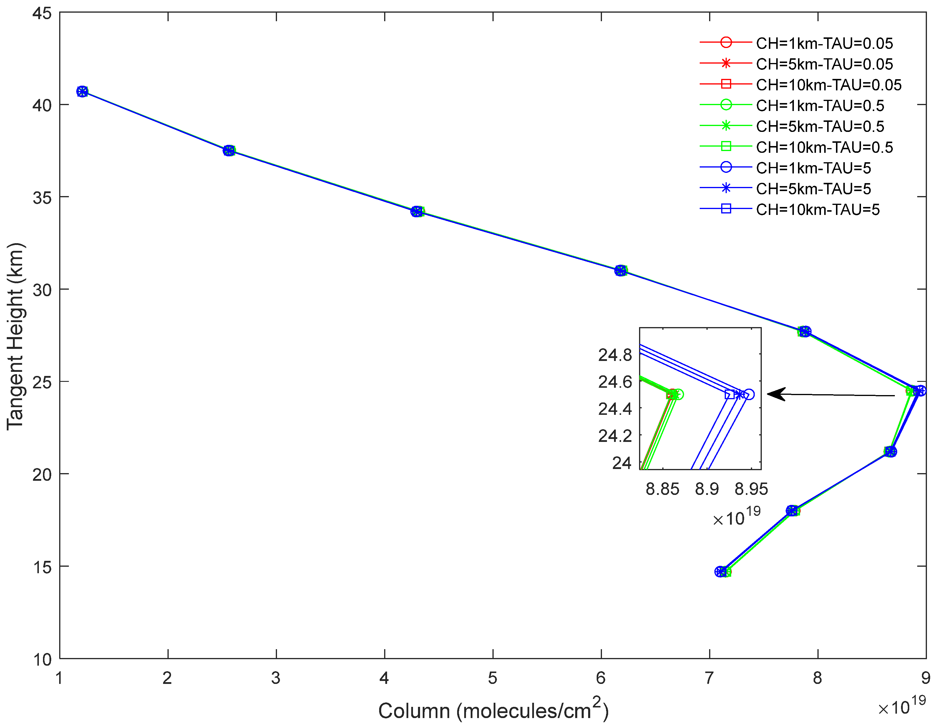
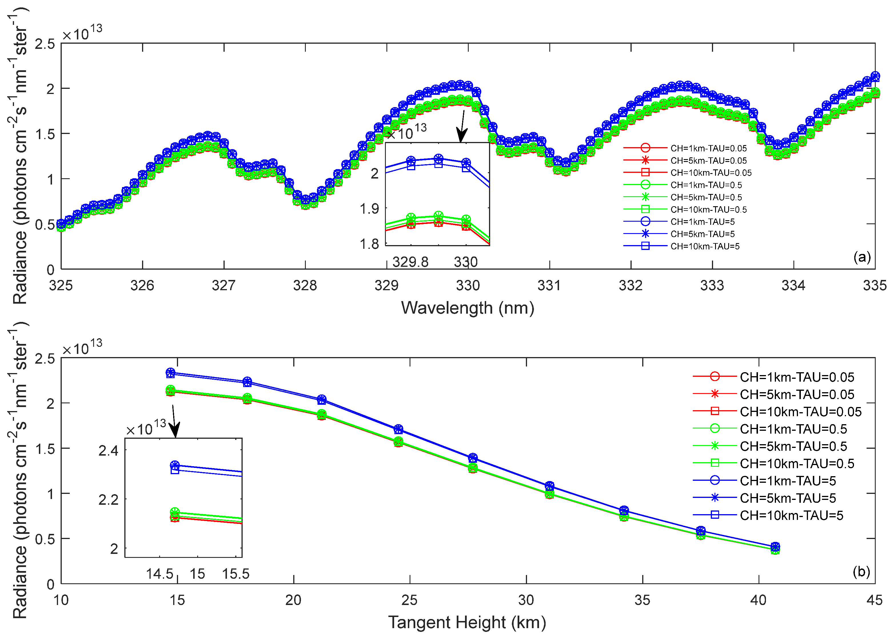
2.3.1. Clouds
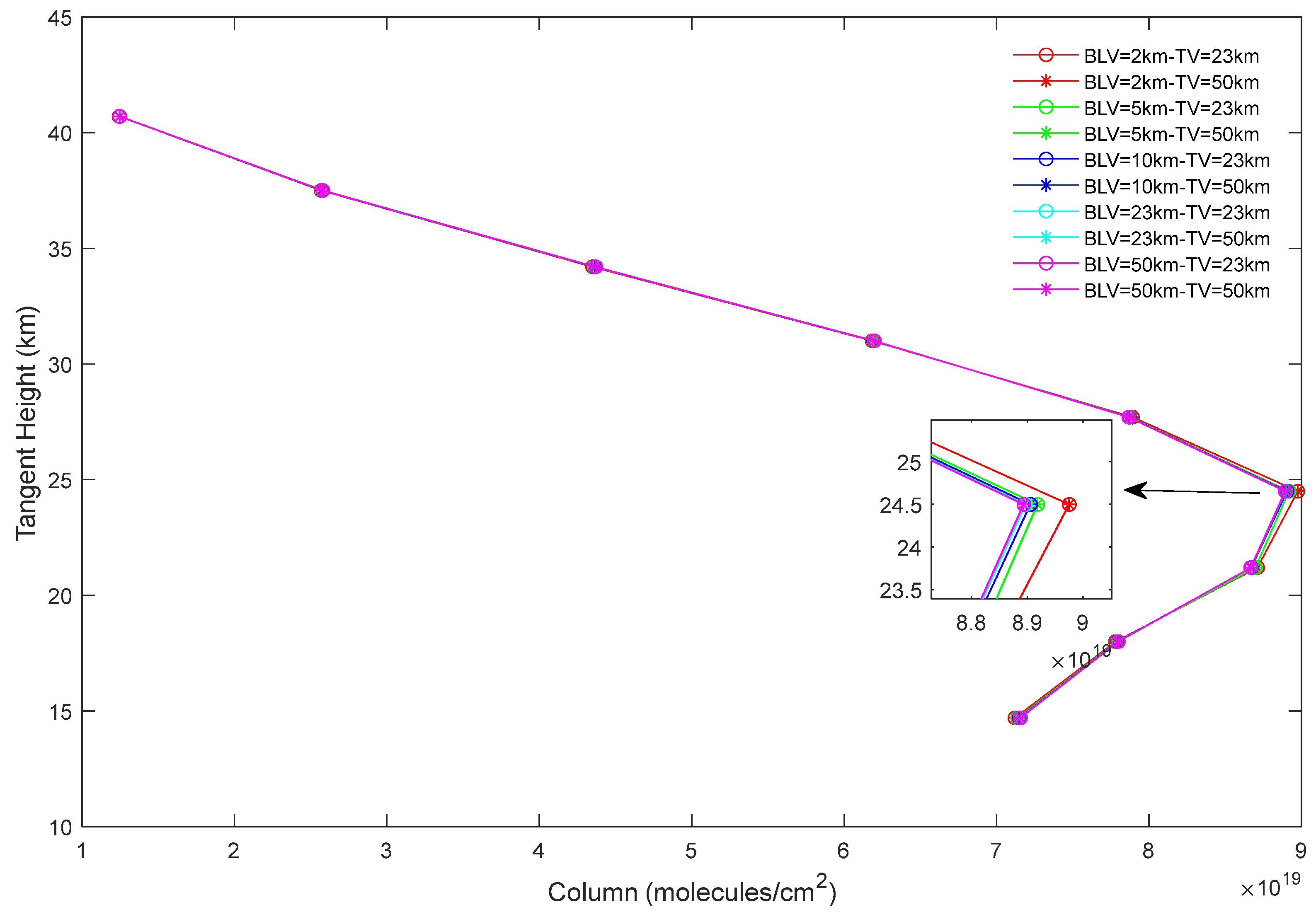
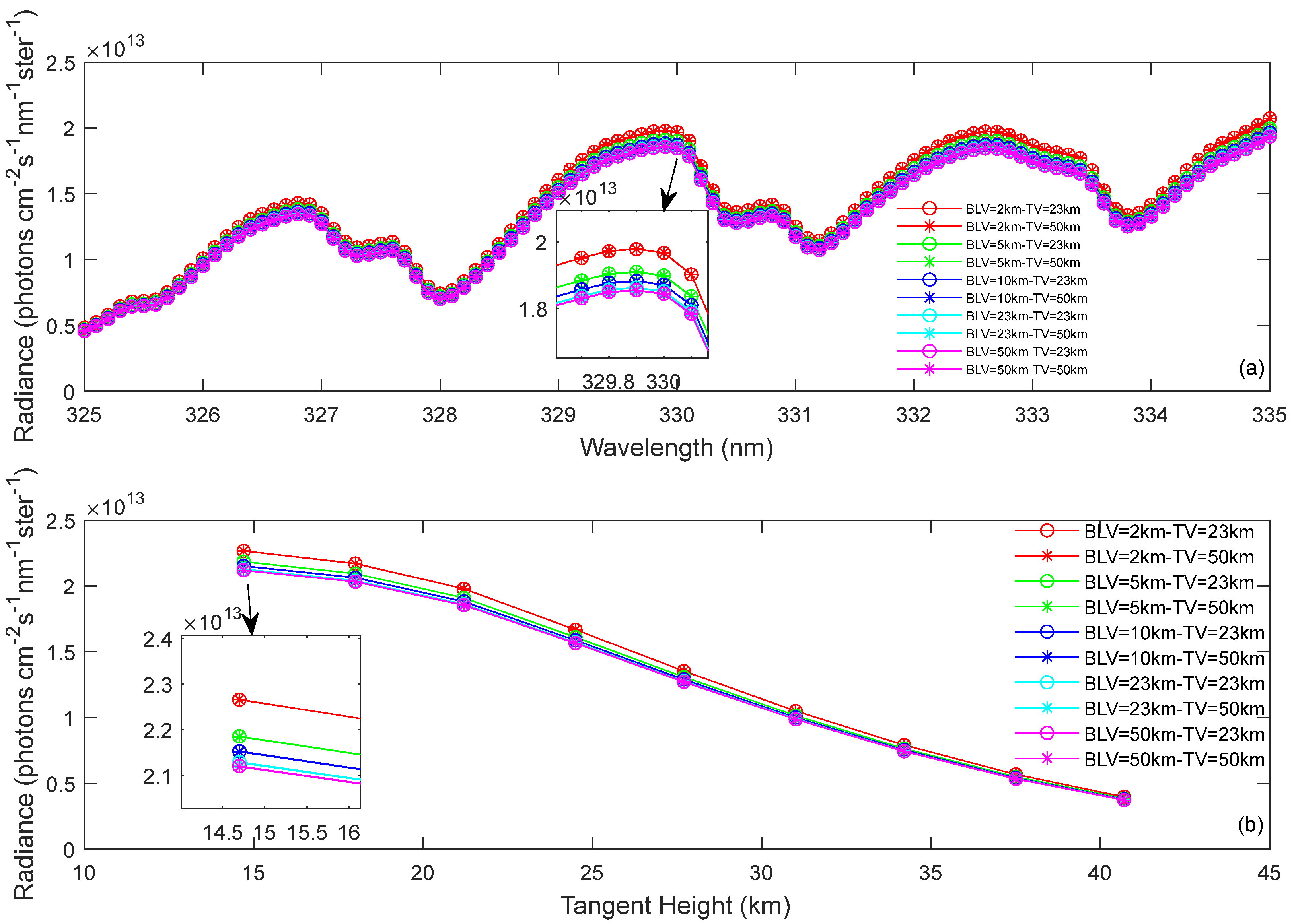
2.3.2. Aerosols
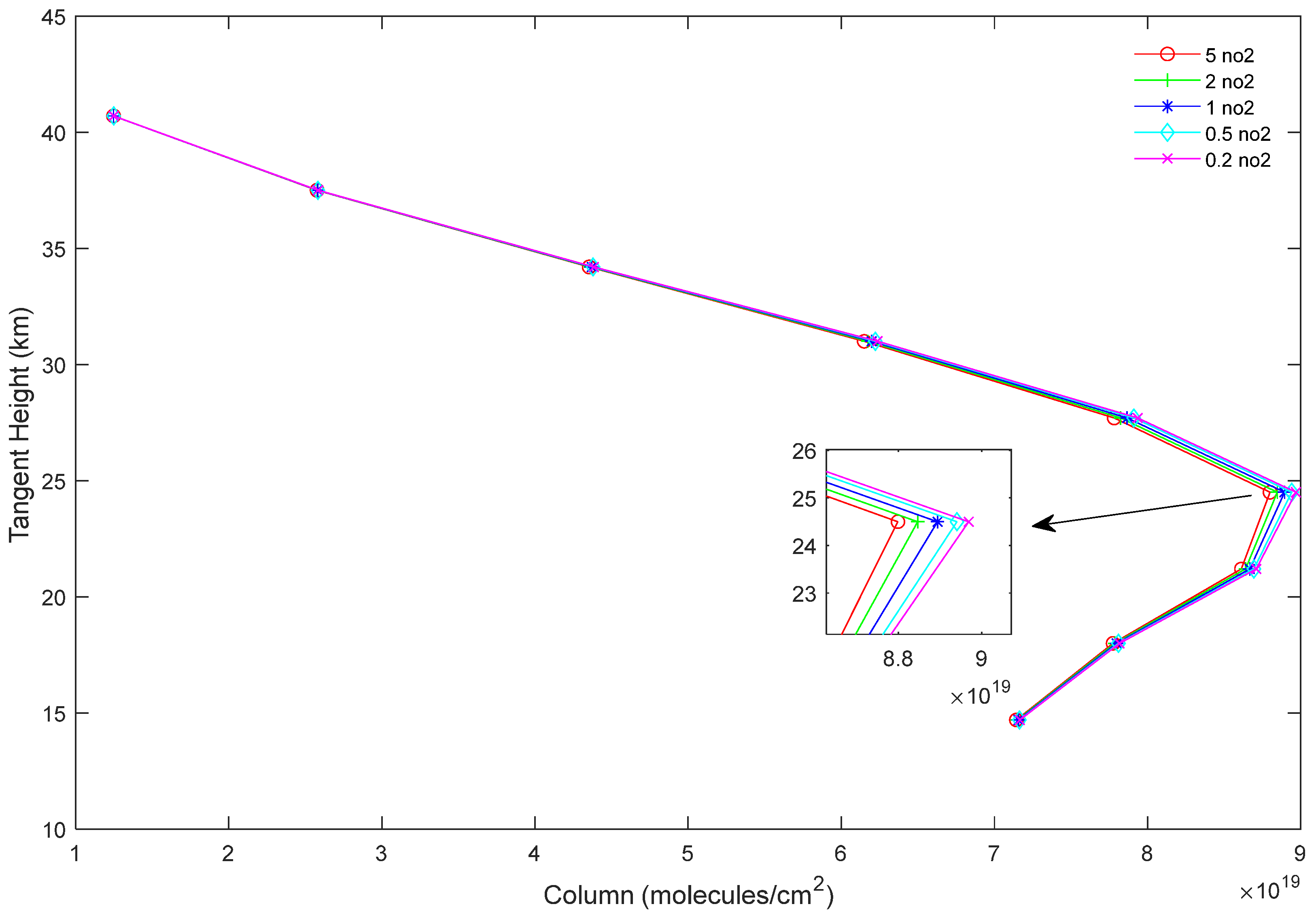
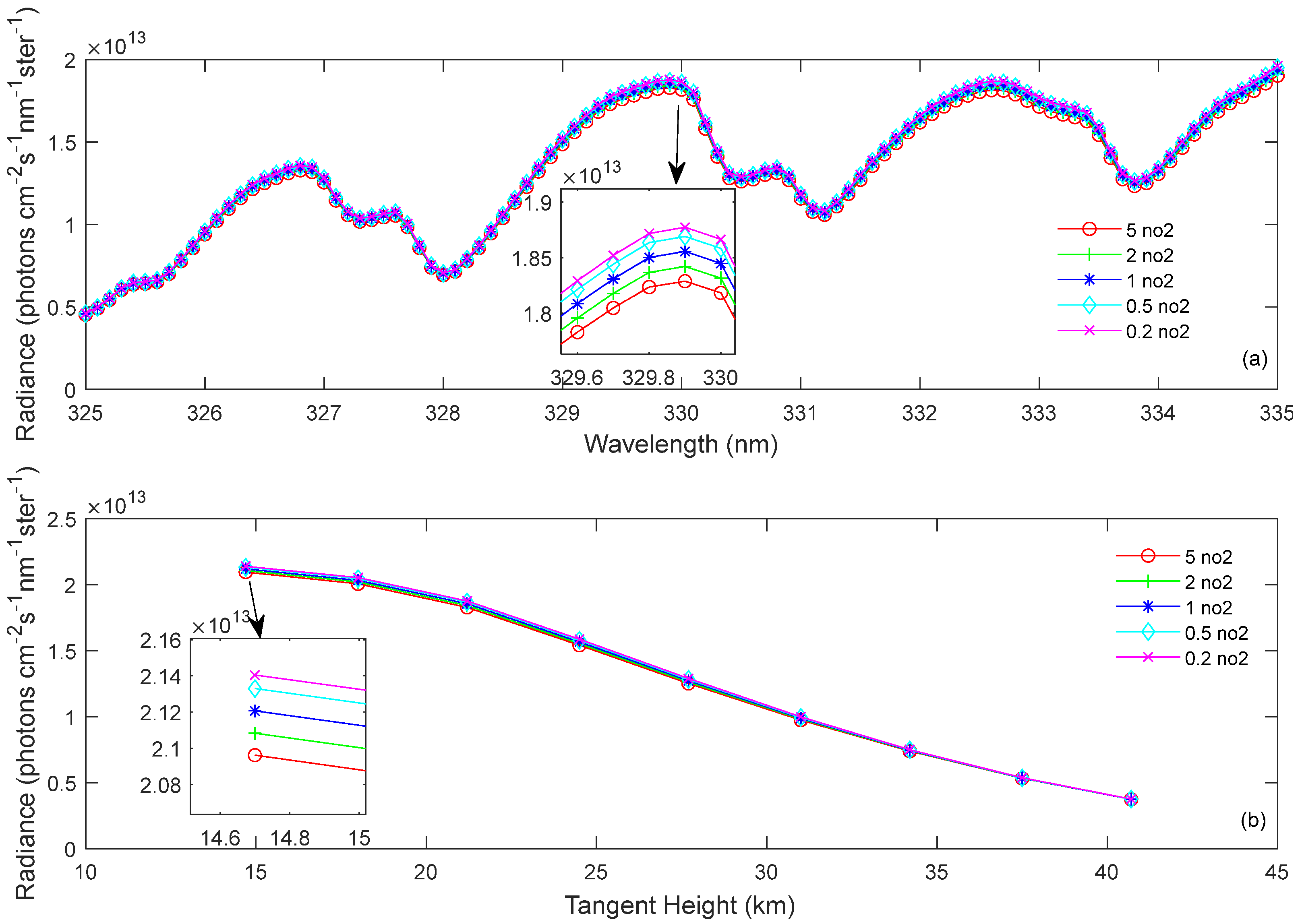
2.3.3. NO2
3. Results and Discussion
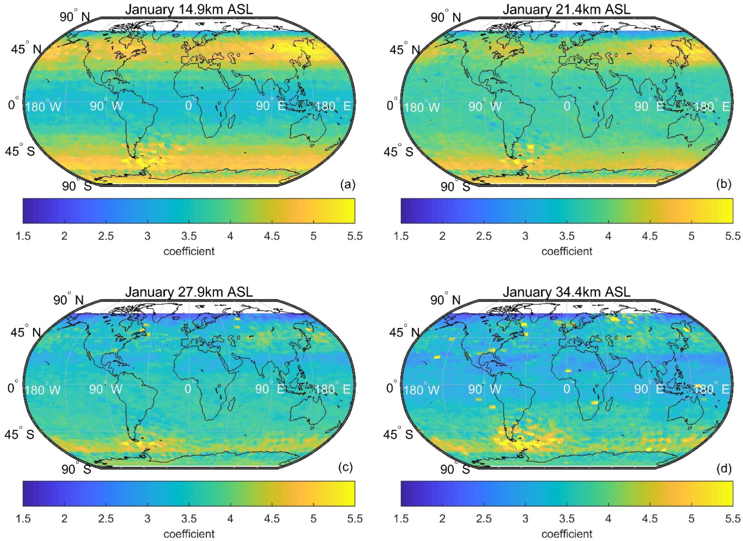
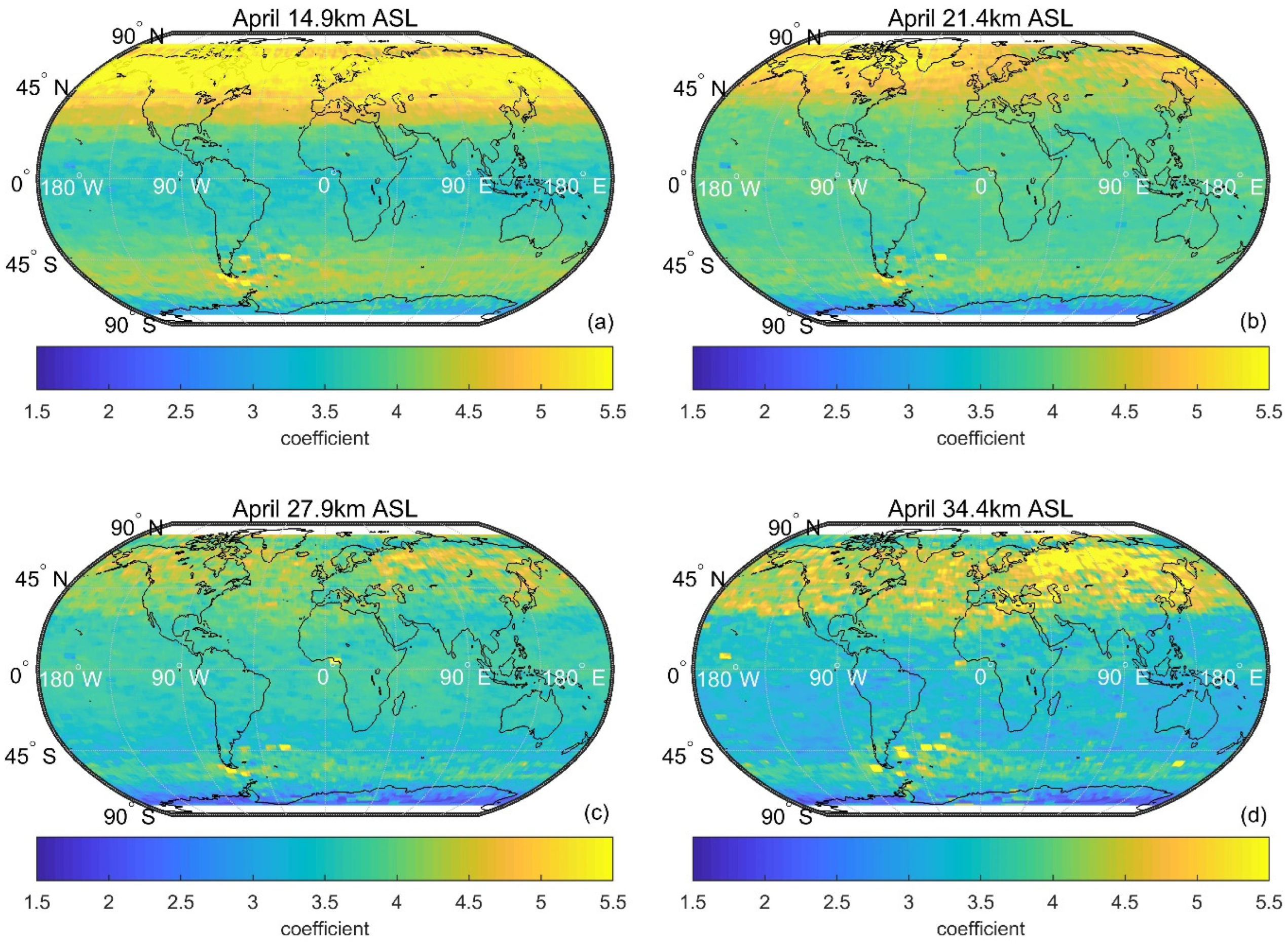
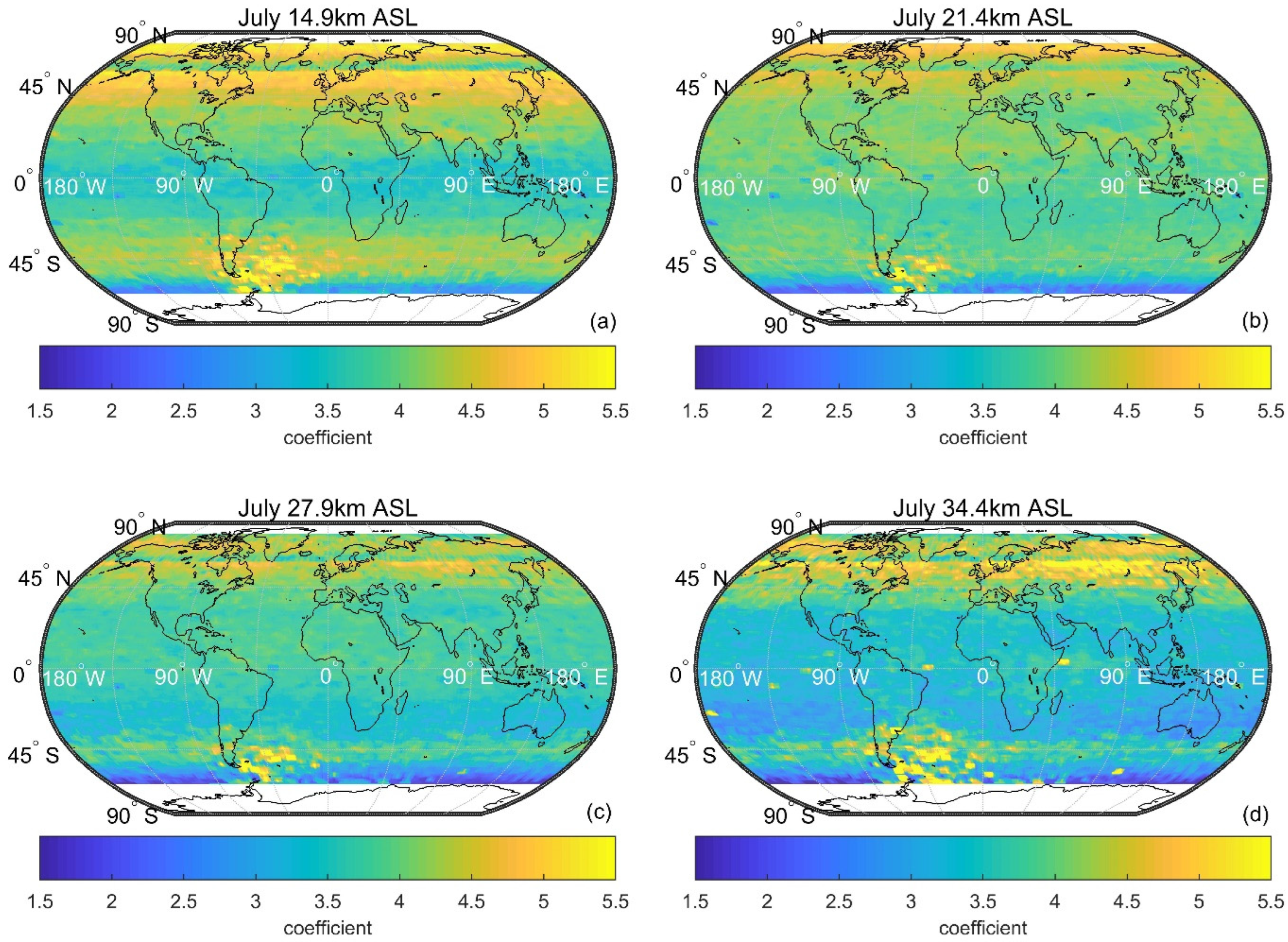
3.1. Global Optical Depth Coefficients (αj)
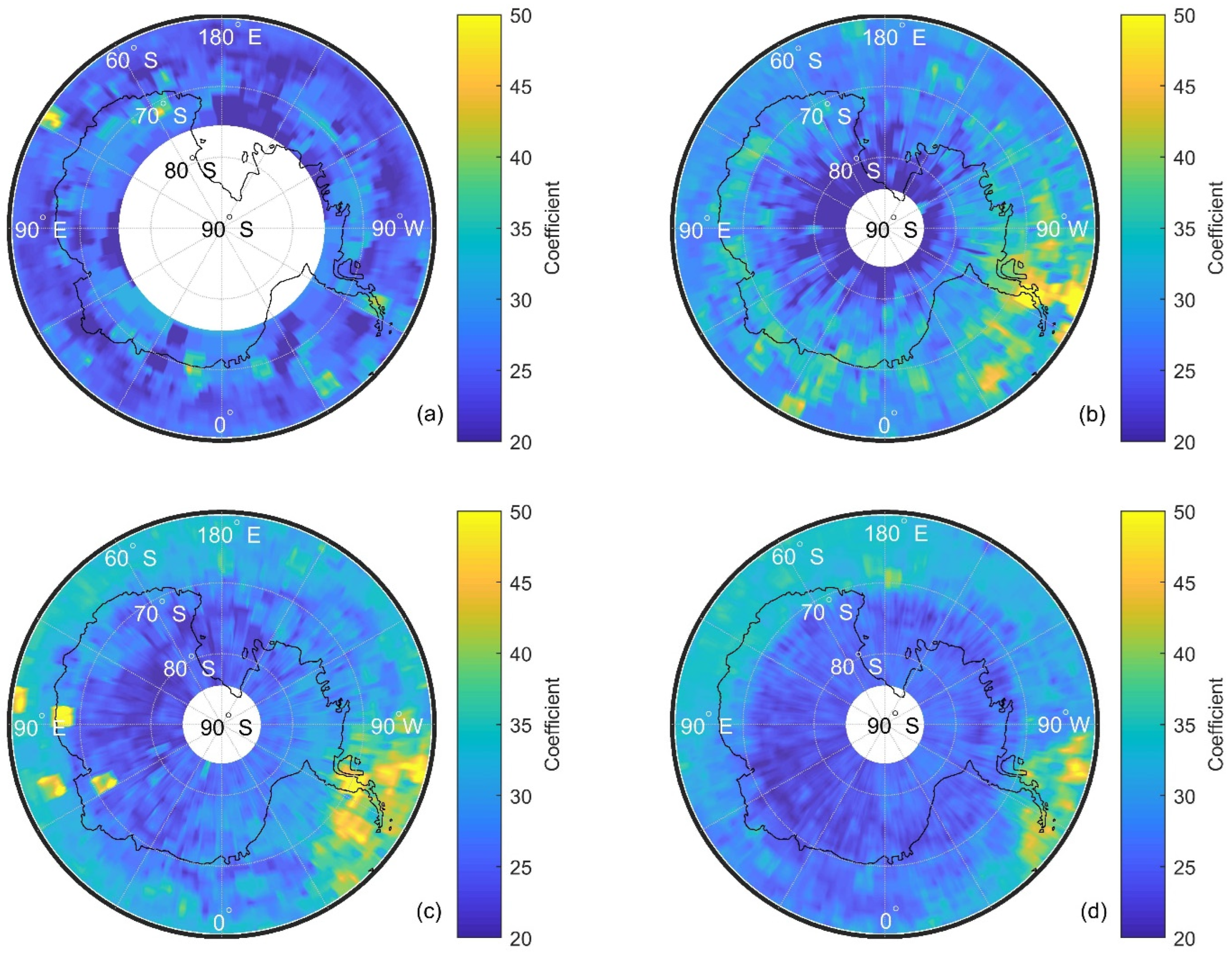
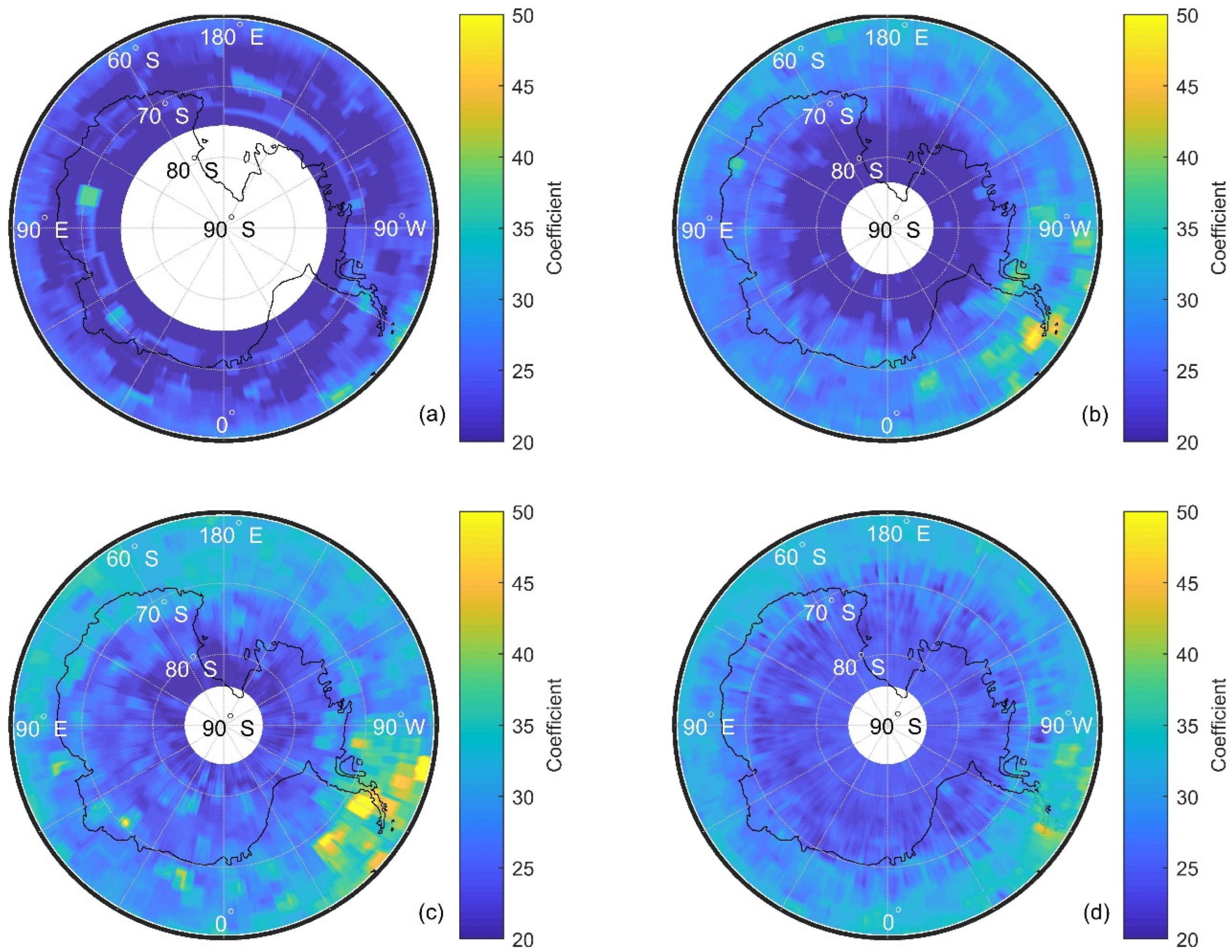
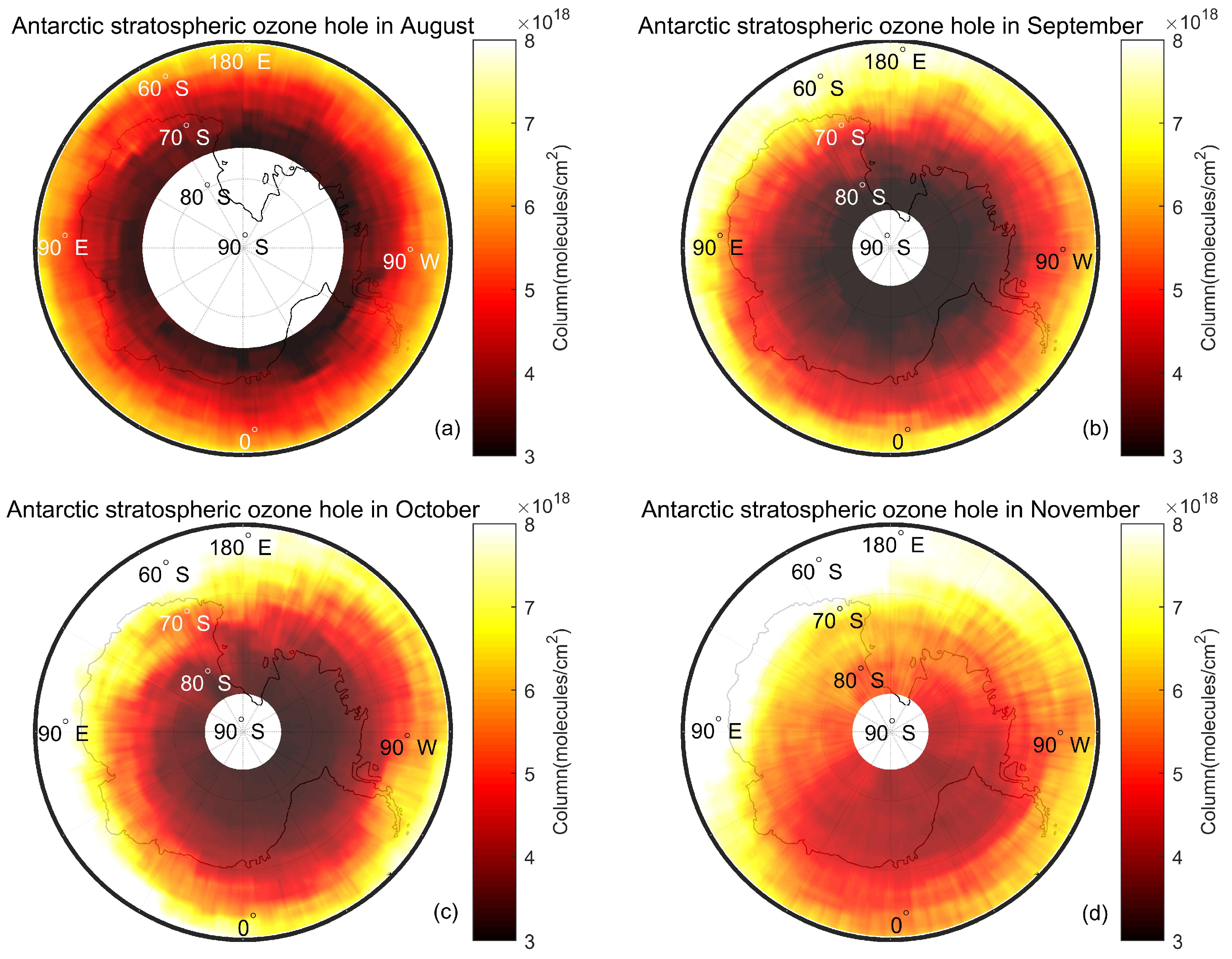
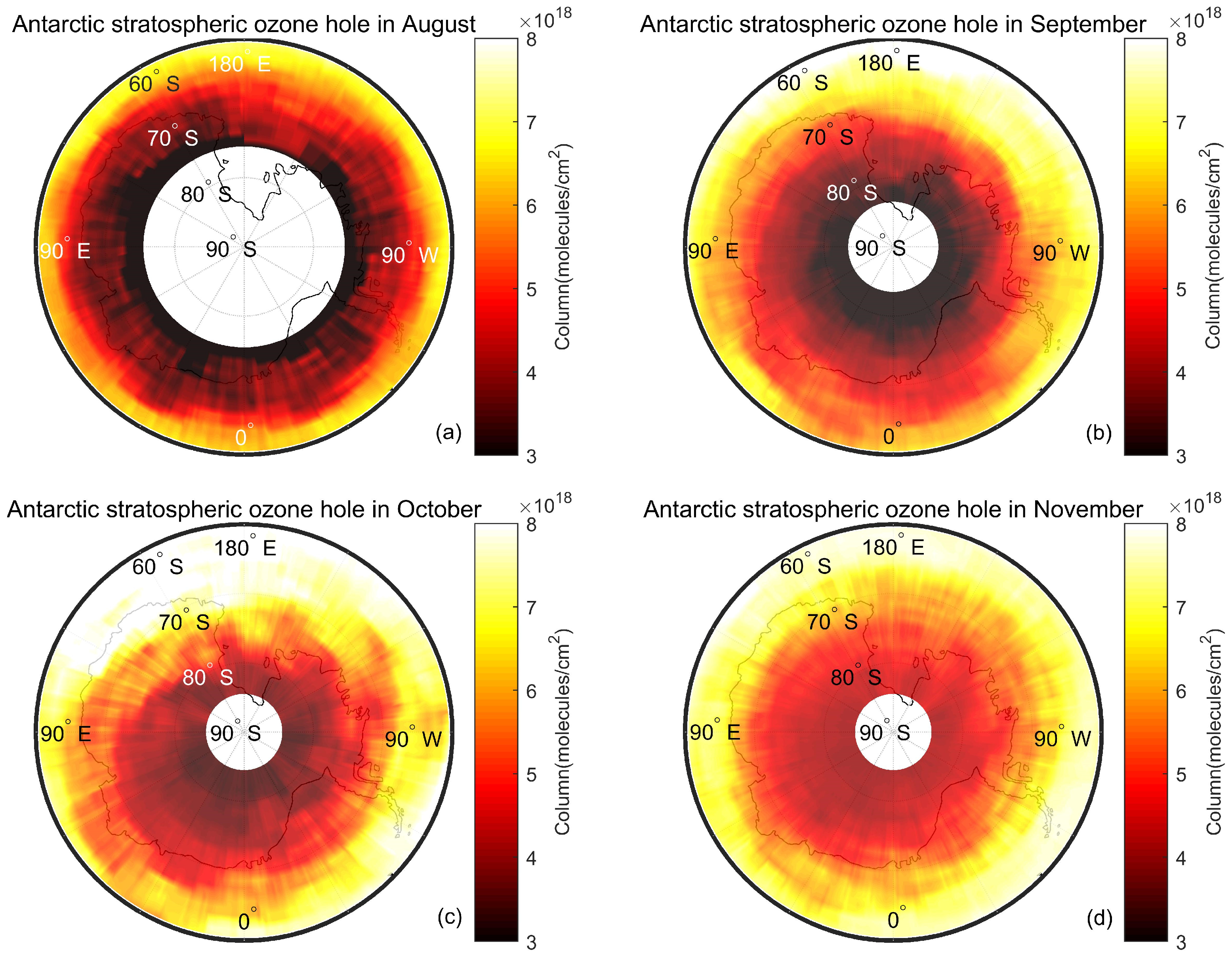
3.2. Antarctic Optical Depth Coefficient (αj) Analysis
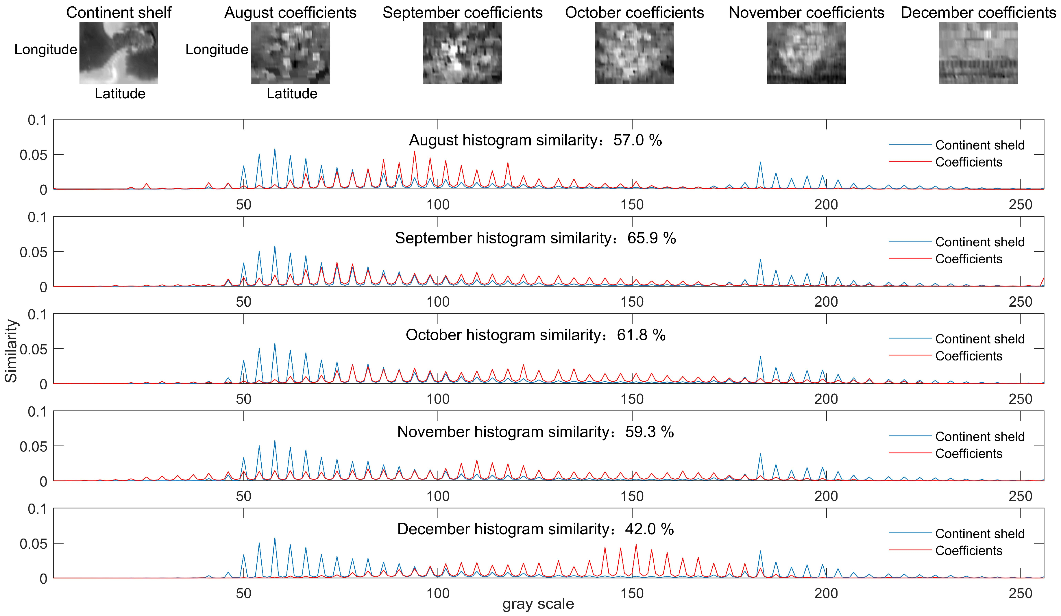
3.3. Relationship between Antarctic Optical Depth Coefficients and Ozone Concentration Gradient Using Statistical Methods
4. Conclusions
Author Contributions
Funding
Data Availability Statement
Acknowledgments
Conflicts of Interest
Appendix A


References
- Sofieva, V.F.; Tamminen, J.; Kyrölä, E.; Mielonen, T.; Veefkind, P.; Hassler, B.; Bodeker, G.E. A novel tropopause-related climatology of ozone profiles. Atmos. Chem. Phys. 2014, 14, 283–299. [Google Scholar] [CrossRef]
- Kuttippurath, J.; Kumar, P.; Nair, P.J.; Chakraborty, A. Accuracy of satellite total column ozone measurements in polar vortex conditions: Comparison with ground-based observations in 1979–2013. Remote Sens. Environ. 2018, 209, 648–659. [Google Scholar] [CrossRef]
- Dhomse, S.S.; Kinnison, D.; Chipperfield, M.P.; Salawitch, R.J.; Cionni, I.; Hegglin, M.I.; Zeng, G. Estimates of ozone return dates from Chemistry-Climate Model Initiative simulations. Atmos. Chem. Phys. 2018, 18, 8409–8438. [Google Scholar] [CrossRef]
- Meul, S.; Dameris, M.; Langematz, U.; Abalichin, J.; Kerschbaumer, A.; Kubin, A.; Oberländer-Hayn, S. Impact of rising greenhouse gas concentrations on future tropical ozone and UV exposure. Geophys. Res. Lett. 2016, 43, 2919–2927. [Google Scholar] [CrossRef]
- Fang, X.; Pyle, J.A.; Chipperfield, M.P.; Daniel, J.S.; Park, S.; Prinn, R.G. Challenges for the recovery of the ozone layer. Nat. Geosci. 2019, 12, 592–596. [Google Scholar] [CrossRef]
- Montzka, S.A.; Dutton, G.S.; Yu, P.; Ray, E.; Portmann, R.W.; Daniel, J.S.; Elkins, J.W. An unexpected and persistent increase in global emissions of ozone-depleting CFC-11. Nature 2018, 557, 413–417. [Google Scholar] [CrossRef]
- Wohltmann, I.; von der Gathen, P.; Lehmann, R.; Maturilli, M.; Deckelmann, H.; Manney, G.L.; Rex, M. Near-complete local reduction of Arctic stratospheric ozone by severe chemical loss in spring 2020. Geophys. Res. Lett. 2020, 47, e2020GL089547. [Google Scholar] [CrossRef]
- Solomon, S.; Garcia, R.R.; Rowland, F.S.; Wuebbles, D.J. On the depletion of Antarctic ozone. Nature 1986, 321, 755–758. [Google Scholar] [CrossRef]
- Wargan, K.; Kramarova, N.; Weir, B.; Pawson, S.; Davis, S.M. Toward a reanalysis of stratospheric ozone for trend studies: Assimilation of the aura microwave limb sounder and ozone mapping and profiler suite limb profiler data. J. Geophys. Res. Atmos. 2020, 125, e2019JD031892. [Google Scholar] [CrossRef]
- Charney, J.G.; Drazin, P.G. Propagation of planetary-scale disturbances from the lower into the upper atmosphere. J. Geophys. Res. 1961, 66, 83–109. [Google Scholar] [CrossRef]
- Conway, J.; Bodeker, G.; Cameron, C. Bifurcation of potential vorticity gradients across the Southern Hemisphere stratospheric polar vortex. Atmos. Chem. Phys. 2018, 18, 8065–8077. [Google Scholar] [CrossRef]
- Varotsos, C.A.; Cracknell, A.P. Remote sounding of minor constituents in the stratosphere and heterogeneous reactions of gases at solid interfaces. Int. J. Remote Sens. 1994, 15, 1525–1530. [Google Scholar] [CrossRef]
- Varotsos, C.A.; Zellner, R. A new modeling tool for the diffusion of gases in ice or amorphous binary mixture in the polar stratosphere and the upper troposphere. Atmos. Chem. Phys. 2010, 10, 3099–3105. [Google Scholar] [CrossRef]
- Matsuno, T. Vertical propagation of stationary planetary waves in the winter Northern Hemisphere. J. Atmos. Sci. 1970, 27, 871–883. [Google Scholar] [CrossRef]
- Waugh, D.W.; Randel, W.J. Climatology of Arctic and Antarctic polar vortices using elliptical diagnostics. J. Atmos. Sci. 1999, 56, 1594–1613. [Google Scholar] [CrossRef]
- Waugh, D.W.; Polvani, L.M. The Stratosphere: Dynamics, Transport, and Chemistry. Geophys. Monogr. Ser. 2010, 190, 43–57. [Google Scholar]
- Waugh, D.W.; Sobel, A.H.; Polvani, L.M. What is the polar vortex and how does it influence weather? Bull. Am. Meteorol. Soc. 2017, 98, 37–44. [Google Scholar] [CrossRef]
- Newman, P.A.; Kawa, S.R.; Nash, E.R. On the size of the Antarctic ozone hole. Geophys. Res. Lett. 2004, 31, 21. [Google Scholar] [CrossRef]
- Domeisen, D.I.; Butler, A.H. Stratospheric drivers of extreme events at the Earth’s surface. Commun. Earth Environ. 2020, 1, 59. [Google Scholar] [CrossRef]
- Manney, G.L.; Livesey, N.J.; Santee, M.L.; Froidevaux, L.; Lambert, A.; Lawrence, Z.D.; Fuller, R.A. Record-low Arctic stratospheric ozone in 2020: MLS observations of chemical processes and comparisons with previous extreme winters. Geophys. Res. Lett. 2020, 47, e2020GL089063. [Google Scholar] [CrossRef]
- Domeisen, D.I.; Martius, O.; Jiménez-Esteve, B. Rossby wave propagation into the Northern Hemisphere stratosphere: The role of zonal phase speed. Geophys. Res. Lett. 2018, 45, 2064–2071. [Google Scholar] [CrossRef]
- Gonsamo, A.; Chen, J.M. Circumpolar vegetation dynamics product for global change study. Remote Sens. Environ. 2016, 182, 13–26. [Google Scholar] [CrossRef]
- Damiani, A.; De Simone, S.; Rafanelli, C.; Cordero, R.R.; Laurenza, M. Three years of ground-based total ozone measurements in the Arctic: Comparison with OMI, GOME and SCIAMACHY satellite data. Remote Sens. Environ. 2012, 127, 162–180. [Google Scholar] [CrossRef]
- Butchart, N. The Brewer-Dobson circulation. Rev. Geophys. 2014, 52, 157–184. [Google Scholar] [CrossRef]
- Weber, M.; Dikty, S.; Burrows, J.P.; Garny, H.; Dameris, M.; Kubin, A.; Langematz, U. The Brewer-Dobson circulation and total ozone from seasonal to decadal time scales. Atmos. Chem. Phys. 2011, 11, 11221–11235. [Google Scholar] [CrossRef]
- Phanikumar, D.V.; Kumar, K.N.; Bhattacharjee, S.; Naja, M.; Girach, I.A.; Nair, P.R.; Kumari, S. Unusual enhancement in tropospheric and surface ozone due to orography induced gravity waves. Remote Sens. Environ. 2017, 199, 256–264. [Google Scholar] [CrossRef]
- Fusco, A.C.; Salby, M.L. Interannual variations of total ozone and their relationship to variations of planetary wave activity. J. Clim. 1999, 12, 1619–1629. [Google Scholar] [CrossRef]
- Auvinen, H.; Oikarinen, L.; Kyrölä, E. Inversion algorithms for recovering minor species densities from limb scatter measurements at UV-visible wavelengths. J. Geophys. Res. Atmos. 2002, 107, ACH-7. [Google Scholar] [CrossRef]
- Rohen, G.J.; von Savigny, C.; Llewellyn, E.J.; Kaiser, J.W.; Eichmann, K.U.; Bracher, A.; Burrows, J.P. First results of ozone profiles between 35 and 65 km retrieved from SCIAMACHY limb spectra and observations of ozone depletion during the solar proton events in October/November 2003. Adv. Space Res. 2006, 37, 2263–2268. [Google Scholar] [CrossRef]
- Corsmeier, U.; Kohler, M.; Vogel, B.; Vogel, H.; Fiedler, F. BAB II: A project to evaluate the accuracy of real-world traffic emissions for a motorway. Atmos. Environ. 2005, 39, 5627–5641. [Google Scholar] [CrossRef]
- Verkruysse, W.; Todd, L.A. Improved method “grid translation” for mapping environmental pollutants using a two-dimensional CAT scanning system. Atmos. Environ. 2004, 38, 1801–1809. [Google Scholar] [CrossRef]
- Pundt, I.; Mettendorf, K.U. Multibeam long-path differential optical absorption spectroscopy instrument: A device for simultaneous measurements along multiple light paths. Appl. Opt. 2005, 44, 4985–4994. [Google Scholar] [CrossRef]
- Pundt, I. DOAS tomography for the localisation and quantification of anthropogenic air pollution. Anal. Bioanal. Chem. 2006, 385, 18–21. [Google Scholar] [CrossRef] [PubMed]
- Hönninger, G.; Von Friedeburg, C.; Platt, U. Multi axis differential optical absorption spectroscopy (MAX-DOAS). Atmos. Chem. Phys. 2004, 4, 231–254. [Google Scholar] [CrossRef]
- Laepple, T.; Knab, V.; Mettendorf, K.U.; Pundt, I. Longpath DOAS tomography on a motorway exhaust gas plume: Numerical studies and application to data from the BAB II campaign. Atmos. Chem. Phys. 2004, 4, 1323–1342. [Google Scholar] [CrossRef]
- Zhu, F.; Si, F.; Zhou, H.; Dou, K.; Zhao, M.; Zhang, Q. Sensitivity Analysis of Ozone Profiles Retrieved from SCIAMACHY Limb Radiance Based on the Weighted Multiplicative Algebraic Reconstruction Technique. Remote Sens. 2022, 14, 3954. [Google Scholar] [CrossRef]
- Livesey, N.J.; Van Snyder, W.; Read, W.G.; Wagner, P.A. Retrieval algorithms for the EOS Microwave limb sounder (MLS). IEEE Trans. Geosci. Remote Sens. 2006, 44, 1144–1155. [Google Scholar] [CrossRef]
- Bovensmann, H.; Burrows, J.P.; Buchwitz, M.; Frerick, J.; Noël, S.; Rozanov, V.V.; Goede, A.P.H. SCIAMACHY: Mission objectives and measurement modes. J. Atmos. Sci. 1999, 56, 127–150. [Google Scholar] [CrossRef]
- Hu, Y.; Yan, H.; Zhang, X.; Gao, Y.; Zheng, X.; Liu, X. Study on calculation and validation of tropospheric ozone by ozone monitoring instrument–microwave limb sounder over China. Int. J. Remote Sens. 2020, 41, 9101–9120. [Google Scholar] [CrossRef]
- Qian, Y.; Luo, Y.; Si, F.; Zhou, H.; Yang, T.; Yang, D.; Xi, L. Total Ozone Columns from the Environmental Trace Gases Monitoring Instrument (EMI) Using the DOAS Method. Remote Sens. 2021, 13, 2098. [Google Scholar] [CrossRef]
- Qian, Y.; Luo, Y.; Dou, K.; Zhou, H.; Xi, L.; Yang, T.; Si, F. Retrieval of tropospheric ozone profiles using ground-based MAX-DOAS. Sci. Total Environ. 2023, 857, 159341. [Google Scholar] [CrossRef] [PubMed]
- Wang, Z.; Chen, S.; Jin, L.; Yang, C. Ozone profiles retrieval from SCIAMACHY Chappuis-Wulf limb scattered spectra using MART. Sci. China Phys. Mech. Astron. 2011, 54, 273–280. [Google Scholar] [CrossRef]
- Loughman, R.P.; Flittner, D.E.; Herman, B.M.; Bhartia, P.K.; Hilsenrath, E.; McPeters, R.D. Description and sensitivity analysis of a limb scattering ozone retrieval algorithm. J. Geophys. Res. Atmos. 2005, 110, D19. [Google Scholar] [CrossRef]
- Rahpoe, N.; Von Savigny, C.; Weber, M.; Rozanov, A.V.; Bovensmann, H.; Burrows, J.P. Error budget analysis of SCIAMACHY limb ozone profile retrievals using the SCIATRAN model. Atmos. Meas. Tech. 2013, 6, 2825–2837. [Google Scholar] [CrossRef]
- Bourassa, A.E.; Degenstein, D.A.; Gattinger, R.L.; Llewellyn, E.J. Stratospheric aerosol retrieval with optical spectrograph and infrared imaging system limb scatter measurements. J. Geophys. Res. Atmos. 2007, 112, D10. [Google Scholar] [CrossRef]
- Corazza, E.; Tesi, G. Tropospheric hydrogen and carbon oxides in Antarctica and in Greenland. Sci. Total Environ. 1995, 160, 803–809. [Google Scholar] [CrossRef]
- Kovář, P.; Sommer, M. CubeSat Observation of the Radiation Field of the South Atlantic Anomaly. Remote Sens. 2021, 13, 1274. [Google Scholar] [CrossRef]
- Zuev, V.V.; Savelieva, E. Antarctic polar vortex dynamics during spring 2002. J. Earth Syst. Sci. 2022, 131, 119. [Google Scholar] [CrossRef]
- Shen, X.; Wang, L.; Osprey, S.; Hardiman, S.C.; Scaife, A.A.; Ma, J. The life cycle and variability of Antarctic weak polar vortex events. J. Clim. 2022, 35, 2075–2092. [Google Scholar] [CrossRef]
- Kang, D.; Im, J.; Lee, M.I.; Quackenbush, L.J. The MODIS ice surface temperature product as an indicator of sea ice minimum over the Arctic Ocean. Remote Sens. Environ. 2014, 152, 99–108. [Google Scholar] [CrossRef]
- Mitchell, D.M.; Scott, R.K.; Seviour, W.J.; Thomson, S.I.; Waugh, D.W.; Teanby, N.A.; Ball, E.R. Polar vortices in planetary atmospheres. Rev. Geophys. 2021, 59, e2020RG000723. [Google Scholar] [CrossRef]


| Parameters | Settings |
|---|---|
| Fitting Interval | 320–340 nm |
| Polynomial | Order 5 |
| Cross sections | |
| O3 | 223 K, 243 K [42] |
| NO2 | 298 K [43] |
| O4 | 293 K [44] |
| HCHO | 297 K [45] |
| BrO | 223 K [46] |
| Ring | Calculated using QDOAS |
| Parameters | Settings |
|---|---|
| Aerosol optical depth scaling | 1 |
| Season | Spring/summer |
| Boundary layer | |
| Aerosol type | Maritime |
| Visibility | 2 km/5 km/10 km/23 km/50 km |
| Humidity | 80% |
| Troposphere | |
| Visibility | 23 km/50 km |
| Humidity | 80% |
| Stratosphere | |
| Aerosol loading | Background |
| Aerosol type | Background |
| Mesosphere | |
| Aerosol loading | Normal mesosphere |
Disclaimer/Publisher’s Note: The statements, opinions and data contained in all publications are solely those of the individual author(s) and contributor(s) and not of MDPI and/or the editor(s). MDPI and/or the editor(s) disclaim responsibility for any injury to people or property resulting from any ideas, methods, instructions or products referred to in the content. |
© 2023 by the authors. Licensee MDPI, Basel, Switzerland. This article is an open access article distributed under the terms and conditions of the Creative Commons Attribution (CC BY) license (https://creativecommons.org/licenses/by/4.0/).
Share and Cite
Xu, Z.; Qian, Y.; Yang, T.; Tang, F.; Luo, Y.; Si, F. Unusual Enhancement of the Optical Depth on the Continental Shelf Depth Latitudinal Variation in the Stratospheric Polar Vortex. Remote Sens. 2023, 15, 4054. https://doi.org/10.3390/rs15164054
Xu Z, Qian Y, Yang T, Tang F, Luo Y, Si F. Unusual Enhancement of the Optical Depth on the Continental Shelf Depth Latitudinal Variation in the Stratospheric Polar Vortex. Remote Sensing. 2023; 15(16):4054. https://doi.org/10.3390/rs15164054
Chicago/Turabian StyleXu, Ziqiang, Yuanyuan Qian, Taiping Yang, Fuying Tang, Yuhan Luo, and Fuqi Si. 2023. "Unusual Enhancement of the Optical Depth on the Continental Shelf Depth Latitudinal Variation in the Stratospheric Polar Vortex" Remote Sensing 15, no. 16: 4054. https://doi.org/10.3390/rs15164054