A Digital Grid Model for Complex Time-Varying Environments in Civil Engineering Buildings

Abstract

The indoor environment is typically a complex time-varying environment. At present, the problem of indoor modeling is still a hot research topic for scholars at home and abroad. This paper primarily studies indoor time-varying space. On the basis of the Beidou grid framework and time coding model, in the first scenario, a local space subdivision framework based on Beidou is proposed. The necessity of local space subdivision framework is analyzed. In the second scenario, based on the time coding model needle, a local temporal subdivision model, more suitable for a short time domain, is proposed. Then, for the spatial modeling of an indoor time-varying environment, an indoor time-varying mesh frame based on global subdivision, local space subdivision, and local time subdivision is proposed. Using this framework, the indoor environment is represented by the space–time grid, and the basic storage data structure is designed. Finally, the experiment of local subdivision coding in the indoor space–time grid, indoor space–time grid modeling, and an organization experiment is carried out using real data and simulation data. The experimental results verify the feasibility and correctness of the encoding and decoding algorithm of local subdivision encoding in space–time encoding and the calculation algorithm of the space–time relationship. The experimental results also verify the multi-space organization and the management ability of the indoor space–time grid model.

1. Introduction

The indoor environment is the most relevant environment for people. According to incomplete statistics, on average every day, most humans spend about 80% of their time indoors [1,2]. Indoor environment modeling is a hot research topic for scholars at home and abroad. It has two characteristics of complexity and time-varying space [3,4,5]. How to better achieve uniformity in modeling, time-varying in expression, and wide application of the indoor environment is the current urgent problem. Therefore, it is not difficult to conclude that the indoor environment modeling method should be able to do the following:

• The environmental modeling method should be able to accurately and effectively process multi-source heterogeneous data so as to achieve the unified modeling and association of multi-source heterogeneous data.
• The time-varying model should be able to dynamically and accurately describe the complex indoor environment and accurately express the time-varying characteristics of objects.
• The time-varying model should have certain construction standards and multi-scale expression capabilities to ensure the sharing of various indoor data among different machines.
• The time-varying model needs to have the ability to support the application of related algorithms, such as path planning.

In order to model the indoor time-varying environment, a time-varying model with the ability to model multi-source heterogeneous data is required. The time-varying model refers to a model with the ability to describe the environment with time-varying characteristics on the space and time scales [6]. The time-varying model has space–time characteristics and can dynamically express the indoor environment. The indoor environment time-varying model, therefore, essentially realizes the spatiotemporal modeling of the indoor dynamic environment.

Aiming at the environment modeling problem of indoor space with strong time-varying characteristics of complex obstacles, this paper proposes a universal indoor time-varying spatial environment modeling method based on the three-dimensional division framework of Earth space, aiming at the environment modeling problem of indoor space with strong time-varying characteristics of complex obstacles. Based on the Beidou grid framework, a local subdivision framework suitable for indoors is proposed under the Beidou grid framework [7,8]. Then, a local temporal partition model suitable for the small-scale temporal domain is proposed under the temporal coding model [9]. The global subdivision, indoor local space subdivision, and local time subdivision models are combined to realize indoor space–time grid modeling and grid representation of obstacle information in indoor scenes. The coding and decoding calculations of the model are studied, and a set of efficient spatial–temporal grid coding and decoding calculation methods are provided. Finally, a set of data storage methods based on the space–time grid is designed, allowing the space–time model to carry multi-source heterogeneous data, and when the physical state of the real object changes, the object information in the space–time model can be dynamically updated. This method is perfectly compatible with time-varying indoor space, characteristics, and allows one to realize the time-varying modeling of the indoor environment.

2. Related Work

At present, the modeling methods for indoor complex environments mainly include geometric modeling, topology modeling, and grid modeling [10,11,12,13]. This paper mainly investigates and analyzes the time-varying extended applications of these methods.

Geometric modeling methods [14,15,16,17,18,19,20] are indoor local modeling methods that describe real indoor space through basic geometric elements. The method uses geometric shapes such as points, lines, and surfaces to describe the size, shape, boundary, etc., of the actual space, as well as all obstacles existing in the space, and usually uses the boundary information of objects or spaces for modeling, for example, the visual view method. The visual graph method connects the starting and ending points with all obstacle vertices to obtain a planning map. Once the planning map is completed, the visual graph method retains all edges that do not intersect with obstacles, finally assigns weights to these edges, and uses these edges, starting, and ending points to form a graph for path planning. Geometric modeling methods are a very simple and intuitive local modeling method which can quickly build indoor space models. When the objects in the modeling space become dense and complex, the computational complexity of the geometric modeling method will be greatly improved. It is difficult to handle extremely irregularly shaped obstacles. When the time-varying characteristics of the object itself are difficult to express through the time equation, the geometric modeling method becomes inapplicable.

Topological modeling methods [21,22,23,24,25,26,27,28] are local modeling methods modeling indoor environments through a graph structure of edges and points [22,23,24]. These points and edges are of practical significance. Topological modeling is essentially a high-level abstraction of space. In topology modeling, edges represent feasible and effective paths in the real world, and points represent the intersections or starting and ending points of these edges. When using the topology map for indoor path planning, the robot strictly follows the path corresponding to the topological edge to reach the corresponding target point. The target point also requires the realistic path corresponding to the topological edge to be safe and reliable. Topological modeling methods are graph data structures. With small storage space and high computational efficiency, topological modeling methods are very beneficial to further application algorithms such as path planning. Since topology modeling is a graph structure, it only considers the connectivity of nodes, requires strong manual intervention for specific topology edge routes, and is difficult to create [9]. Although the time-varying topology graph has the ability to express the time-varying environment, its ability to express the time-varying environment is limited. The topological map is an abstract expression. This high abstraction also leads to a lack of information, allowing edge and point information to be obtained, and other information is omitted.

Raster modeling methods [29,30,31,32] are a common indoor local modeling method which expresses the environment by using grids of uniform size. It divides the indoor space into two categories, namely the passable free grids and the impassable obstacle grids. In this method, the grid is used as the basic unit to carry the space. The larger the grid scale, the rougher the environmental modeling and the poorer the planning quality [29]. The smaller the grid scale, the finer the environmental modeling, but raster modeling methods will bring a lot of storage space and increase the algorithm complexity. The relationship between the grids is clear and clear, which is conducive to the application of subsequent algorithms such as path planning. The planning space can be converted into the form of an array or matrix, which is very convenient for data storage and processing. This method is the most widely used local modeling method. The expression is simple. The environment modeling ability is strong. It can express arbitrarily complex obstacles [30] and can construct fine indoor maps. After the time interval attribute is introduced into the grid, the indoor environment can be expressed dynamically. There is a lack of unified construction standards. For example, different indoor mobile robots often need to build local grid maps according to their own scales, making it difficult to share data under the grid modeling method between robots.

In summary, there are four requirements for indoor environment modeling: unified modeling and correlation of multi-source heterogeneous data, dynamic and accurate representation of the time-varying characteristics of objects, ability to construct standard and multi-scale representations, support for path planning, and other related algorithm applications. The current three methods (geometric modeling, topological modeling, and raster modeling) only meet some of the requirements and are not able to meet all of them at the same time. Geometric modeling methods do not satisfy the need for a dynamically accurate representation of the time-varying characteristics of an object. Topological modeling methods have the ability to express the time-varying environment, but the ability to express time-varying space is limited. Raster modeling methods construct local raster maps according to their own scale needs and lack a unified construction standard.

3. Materials and Methods

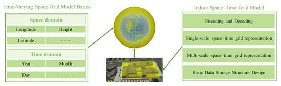
3.1. Time-Varying Space Grid Model Basics

3.1.1. Beidou Grid Model

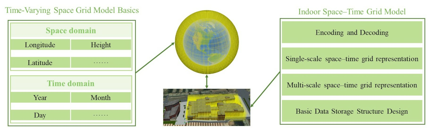
Beidou [33,34,35] adopts latitude and longitude subdivision, which has the characteristics of non-overlapping boundaries, orthogonal grids, consistent longitude and latitude, good compatibility with traditional data specifications, and better realizes the division of spherical space. On the basis of inheriting these characteristics, Beidou expands the Beidou two-dimensional grid in the height dimension to complete the division of spherical space. A 2D mesh frame is a special case of a 3D mesh frame. The Beidou 3D grid divides the Earth space and selects the geodetic height of the CGCS2000 geodetic coordinate system (as the elevation direction) through strict recursive division, which is divided into a multi-level three-dimensional grid system covering the whole world. In order to make the size of the mesh unit (division voxel) a binary integer, which is easily compatible with other data, Beidou realizes the recursive octree of integer degree, minute, and second through three Earth expansions (expand the Earth space to 512° × 512° × 512°, 1° to 64′, 1′ to 64″), as shown in Figure 1a.

The Beidou grid is divided into 32 levels, and the 0-level grid corresponds to the entire Earth’s three-dimensional space, which is defined as: In the Earth’s three-dimensional space based on latitude and longitude coordinates, the 512° square is coincident with its origin (the intersection of the equator and the prime meridian), the longitude space is extended from [−90,90]° to [−256°,256°], the latitude space is extended from [−180°,180°] to [−256°,256°], and the height of space is 0° from the center of the Earth and goes up to 512°; as the level deepens, the space is continuously divided into 8 equal parts until 1/2048 s. After multi-level division, the space up to 50,000 km and the three-dimensional space down to the center of the Earth are divided into three-dimensional grids of different granularities. Figure 1b shows the grid size of each level of Beidou and its approximate scale around the equator. Levels 10–15 are graded grids, levels 16–21 are second-level grids, and levels 22–32 are sub-second grids. The hierarchical grid root node is a 9-level grid, and the second-level grid root node is a 15-level grid.

3.1.2. Time-Division Coding Model

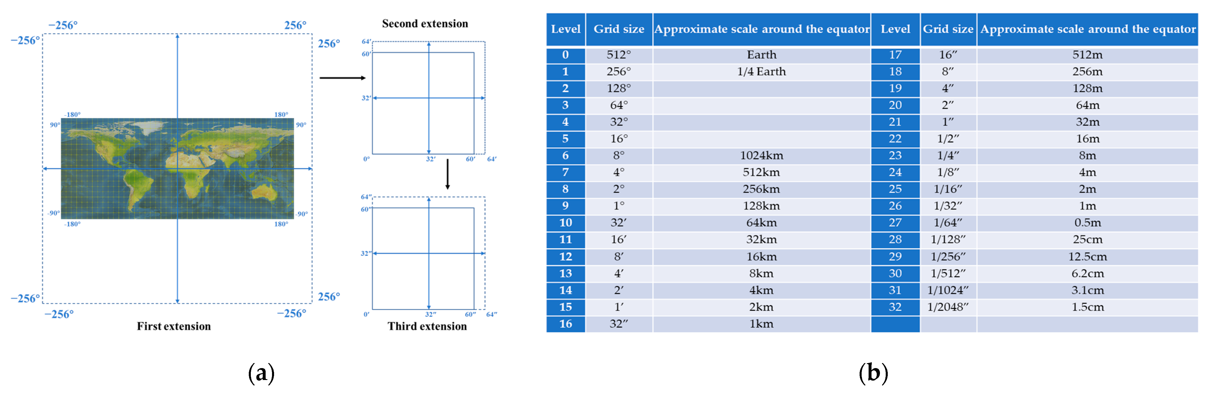
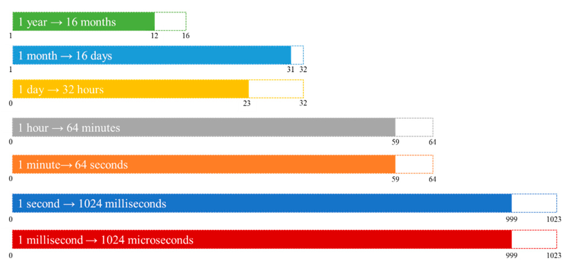
The time-division coding model refers to the multi-scale temporal segmentation coding model. In 2016, Wang Lin proposed a set of time-division coding models in his doctoral dissertation. The essence of this subdivision model is the time binary tree subdivision: in the limited time domain (65,536 BC to 65,535 AD), the binary tree subdivision of year, month, day, hour, minute, and second are realized by extending the time base 7 times (1 year to 16 months, 1 month to 32 days, 1 day to 32 h, 1 h to 64 min, 1 min to 64 s, 1 s to 1024 milliseconds, and 1 millisecond is extended to 1024 microseconds). A time-slice binary tree is formed from the time scale of 60,000 years after BC to the time scale of 1 microsecond, thus forming a multi-scale and unified discrete-time coding system. The multi-scale time division code consists of 64 levels, and this code adopts the Gregorian calendar standard and the UTC time standard [9,36]. The seven virtual extensions of time are shown in Figure 2.

3.2. Indoor Local Space Division Model

The division principle of indoor local space division model: firstly, the necessity of indoor local space division is explained. Due to the interference of indoor GPS and other global position signals by walls and so on, it is difficult to accomplish real-time accurate latitude and longitude positioning indoors. At present, the coordinates obtained by mobile robots through sensors and other equipment for indoor positioning are all three-dimensional Cartesian coordinate systems under the local Cartesian coordinate system, basically using meters as the unit of measurement of distance. Although local coordinates can be used to solve position information such as latitude and longitude through control points using relative coordinates, this introduces too many conversion calculations, which makes the computational efficiency of indoor frames greatly reduced, so it is very necessary to adopt local coordinate systems in indoor environments. Moreover, the grid size of the globally dissected grid varies in different latitude and longitude grid sizes, and the grid size under the indoor localized dissections is determined and does not affect the size of the grid itself because of the location. The grid size of local profiling is uniform.

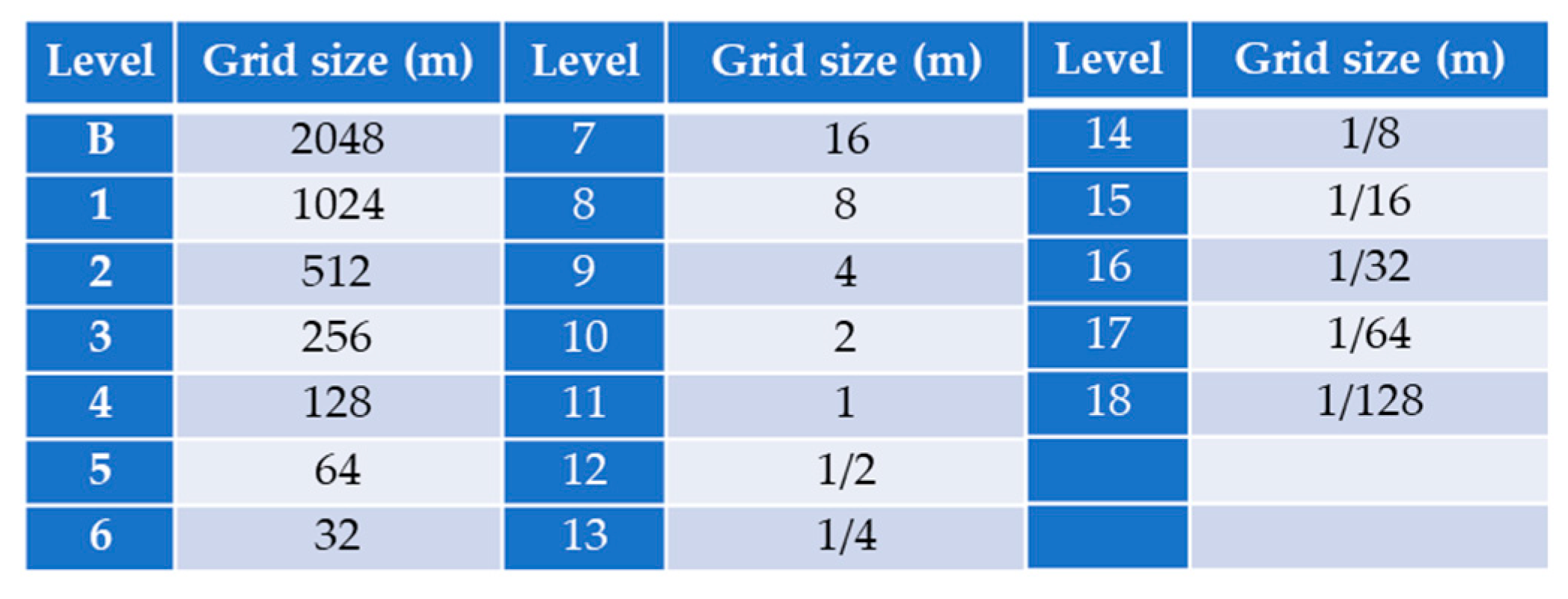
The indoor local meshing framework in this paper is based on Beidou meshing. The grid center of an indoor Beidou mesh is used as the origin of the indoor local coordinate system, and the latitude and longitude directions of the center point are used as the X-axis direction and the Y-axis direction, respectively. The Z-axis of the local coordinate system adopts the CGCS2000 geodetic elevation system. This is consistent with the Beidou framework and can be converted to and from the global geographic coordinate system. In terms of subdivision ideas, indoor local mesh subdivision also draws on the idea of Beidou subdivision framework. In essence, it is still the octree division of the grid. Figure 3 shows the levels of indoor partial division.

In indoor local meshing, the big difference between Beidou and indoor local grid is, for a known global mesh, the size of the world is known. Since the grid range obtained by the actual division of each indoor space is different, the indoor local grid needs to be divided according to the size of the real indoor space. On the virtual grid, the virtual grid of Beidou is a real geographic space that does not exist due to the expansion of degrees, minutes, and seconds of latitude and longitude. Since the actual indoor space is limited, some grids of the indoor local grid generated during the subdivision process have no real meaning beyond the geographical scope of the indoor space.

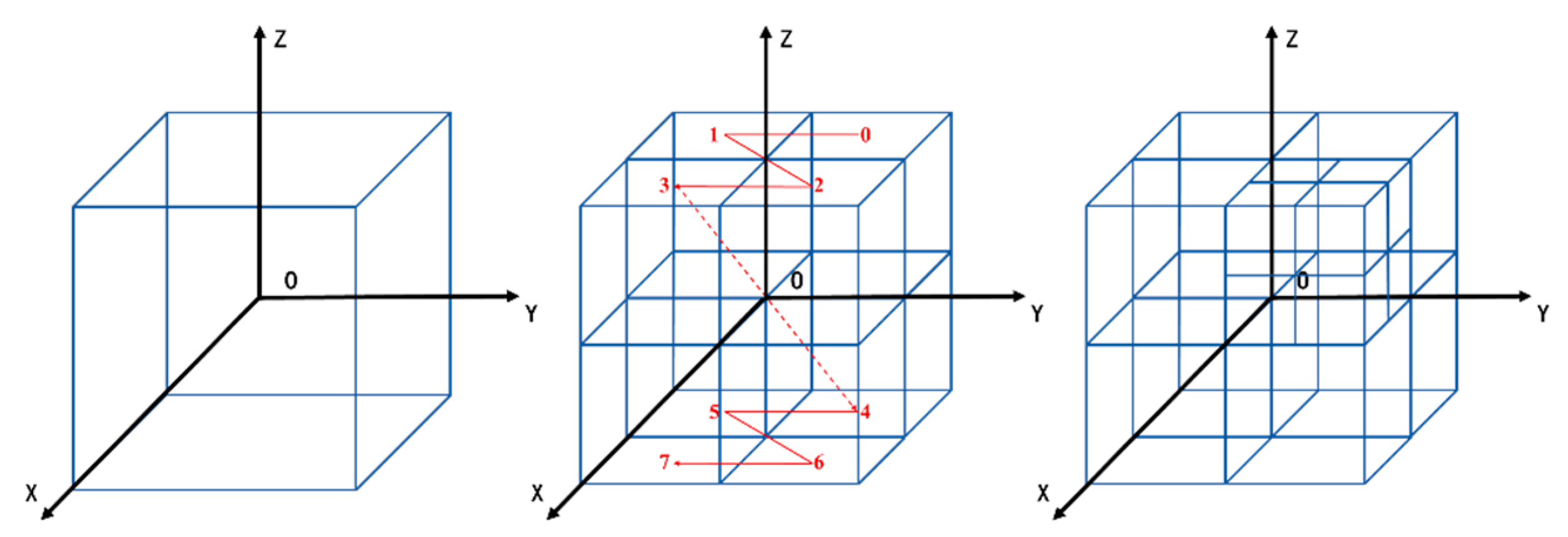
The encoding method of indoor local space division model: the encoding method of the indoor local grid also refers to the encoding method of Beidou, but different from the Beidou subdivision framework, there is no quadrant code subdivision for indoor local grid subdivision. For indoor local meshing, the three-dimensional Z-sequence of each mesh is the same, and it is coded according to the X-axis, Y-axis, and Z-axis from small to large, as shown in Figure 4. Grids at level 0 are coded B, and subsequent levels are coded with digital records.

3.3. Indoor Local Time Division Model

Although the time coding introduced above can fully cover the time domain from 65,536 BC to 65,535 AD, for indoor space, the time scale covered by this coding model is too large, causing essentially coding redundancy and unnecessary storage consumption. Therefore, it is necessary to use the local form, and it is more convenient and efficient to use a short local time code.

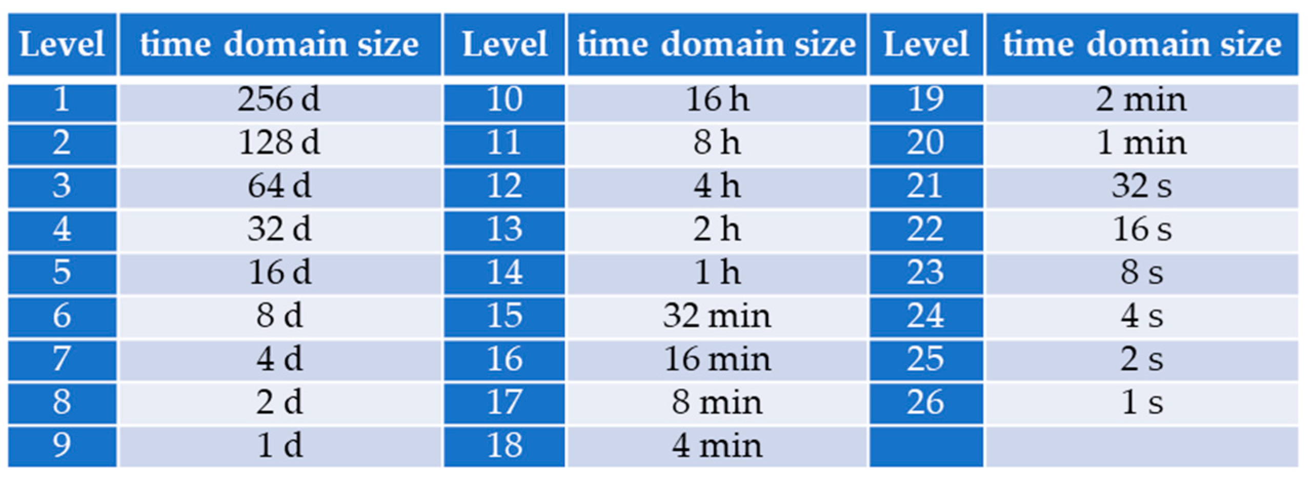
The division principle of indoor local time division model: referring to the Beidou time encoding model, the difference in this article’s method is that in order to facilitate the calculation of time relationships, the month unit has been removed, and in the local time subdivision model, there are only five scales: day, hour, minute, and second. The virtual expansion of this year is to expand from the original 16 months to 512 days. In addition, considering the smooth transmission of time data between adjacent years, especially within the extended 512 days, including 64 days at the end of the previous year and 64 days at the beginning of the next year. Taking a normal year as an example, 1–64 days out of 512 are the last 64 days of the previous year, 65–429 days are the 365 days of the current year, and 430–493 days are the first 64 days of the next year. The remaining days are considered virtual delays. Through this approach, time data can be more effectively smoothed into annual data conversion. In time domain partitioning, indoor local time partitioning models also use binary partitioning to partition time. The level of indoor time division is shown in Figure 5.

The encoding method of indoor local time division model: since the model itself adopts binary division, in each level of division, the time domain with the earlier time is coded as 0, and the time domain with later time is coded as 1. In the form of encoding, 32-bit integer encoding is used. When using this encoding, the 1st to 26th bits in the 32 bits are used to store the time domain codes of the 26th to the 1st level, the 27th bit indicates whether the year in which the code is located is a leap year, and the 28th to 32nd bits indicate the level of time coding.

3.4. Indoor Space–Time Grid Model

A space–time grid refers to a grid that not only contains spatial information such as its own spatial position and size but also contains temporal information such as its own time interval. For the spatial–temporal grid modeling of the indoor environment, in essence, the indoor local space subdivision framework and the local time subdivision model are used to separately model the indoor space and time. The two are then combined into one to generate a space–time grid with both temporal and spatial attributes.

3.4.1. Encoding and Decoding of Indoor Space–time Grid

The encoding and decoding of indoor spatiotemporal trellis coding is the basis for using indoor spatiotemporal trellis coding. Through encoding and decoding, the rapid mutual conversion from indoor local coordinate points to indoor local spatial grid coding, indoor local spatial grid coding to indoor local point coordinates, time domain to local time coding, and local time coding to time domain can be realized. The encoding gives the spatial voxel and the temporal voxel unique corresponding identities. Indoor spatiotemporal grid coding is composed of Beidou coding, local spatial coding, and local temporal coding. For the mutual conversion between latitude, longitude, and Beidou encoding, because of Zhou’s work [33], this article will not discuss these related algorithms.

The indoor local space code generation algorithm refers to converting a certain local coordinate under the indoor local into a unique corresponding local space code. For any point P in the local coordinate system with the center of a Beidou voxel as the origin, if the local coordinates of the point are known, the grid code corresponding to the point P can be calculated according to the indoor local space subdivision model. The specific calculation process is as follows Algorithm 1.

Algorithm 1: Local Coordinate Transcoding Algorithm.

Require: Local coordinates $[X,Y,Z]$ of any point, Slice level $level\ge 1$ Ensure: The binary integer encoding ${Code}_x$,${Code}_y$,${Code}_z$ of $[X,Y,Z]$ under the $level$ Step 1:${Code}_x={Code}_y={Code}_z=0, dis=1024, l=1 x=X+1024, y=Y+1024, z=Z+1024$ Step 2: When $l\le level$; ${Code}_x={Code}_x\ll 1$; ${Code}_y={Code}_y\ll 1; {Code}_z={Code}_z\ll 1$    if $x\ge dis$; ${Code}_x={Code}_x+1$; $x=x-dis$    if $y\ge dis$; ${Code}_y={Code}_y+1$; $y=y-dis$    if $z\ge dis$; ${Code}_z={Code}_z+1$; $z=z-dis$    $dis=dis/2$ Step 3: ${Code}_x={Code}_x\ll \left(18-level\right),{Code}_y={Code}_{xy}\ll \left(18-level\right); {Code}_z={Code}_z\ll (18-level)$ Step 4: return ${Code}_x, {Code}_y, {Code}_z$

Decoding refers to restoring a local spatial subdivision code to the size corresponding to its real local coordinates and the corresponding local grid. Local time coding refers to converting a given time domain into a specific and unique code through certain coding rules. The time code is the identity of the local time domain. Before generating the local time code, it is necessary to format the time data first. Since the local time subdivision model only considers days, hours, minutes, and seconds, for example, when the input is 10 January, 12:10:00, it should be converted to 10 days, 12:10:00. When performing day conversion, it is necessary to consider the leap year of the year. The specific generation method for the time code corresponding to the time point is as follows Algorithm 2.

Algorithm 2: Time to Local Time Coding Algorithm.

Require: Whether the year at this time point is a leap year $isleap$ (1 is yes, 0 is not), time point A day B hour C minute D second, the level of $level$ $(1\le level\le 26$) Ensure: Decimal integer time code ${Code}_{time}$ at level $level$ at this point in time Step 1:$days=A+64, hours=B, mins=C, secs=D$,$x=X+1024, y=Y+1024, z=Z+1024$ Step 2: $\mathbf{W}\mathbf{h}\mathbf{e}\mathbf{n} 1\le level\le 9;$ ${Code}_{time}={Code}_{time}\ll 1$; ${Code}_{time}={Code}_{time}+int\left(days/(512/2^{level})\right); days=days mod (512/2^{level})$ Step 3: $\mathbf{W}\mathbf{h}\mathbf{e}\mathbf{n} 10\le level\le 14;{Code}_{time}={Code}_{time}\ll 1$; ${Code}_{time}={Code}_{time}+int\left(hours/(32/2^{level-9})\right); hours=hours mod (32/2^{level-9})$ Step 4: $\mathbf{W}\mathbf{h}\mathbf{e}\mathbf{n} 15\le level\le 20;{ Code}_{time}={Code}_{time}\ll 1$; ${Code}_{time}={Code}_{time}+int\left(mins/(64/2^{level-14})\right); mins=mins mod (64/2^{level-15})$ Step 5: $\mathbf{W}\mathbf{h}\mathbf{e}\mathbf{n} 21\le level\le 26;{ Code}_{time}={Code}_{time}\ll 1$; ${Code}_{time}={Code}_{time}+int\left(secs/(64/2^{level-20})\right); secs=secs mod (64/2^{level-21})$ Step 6: return ${\left(level\ll 27\right)+\left(isleap\ll 26\right)+(Code}_{time}\ll (26-level))$

The decoding of the time code can convert the decimal code into corresponding specific time information. For any decimal time code, a decoding algorithm can be used to decode it to obtain the corresponding day, hour, minute, and second. If there are requirements such as months, the days can be further converted into months and days. The decoding algorithm for the local time coding is as follows Algorithm 3.

Algorithm 3: Local Time Decoding Algorithm.

Require: decimal integer time encoding ${Code}_{time}$ Ensure: The time point corresponding to this code is days, hours, points, mins, minutes, secs, seconds, whether it is a leap year $isleap$ (1 is yes, 0 is not), and the division level is $level$ Step 1: $days=0, hours=0, secs=0, level={Code}_{time}\gg 27,isleap=\left({Code}_{time}\gg 26\right) mod 2,$ $Code={Code}_{time}\gg (26-level)$ Step 2:$\mathbf{W}\mathbf{h}\mathbf{e}\mathbf{n} 21\le level\le 26;$ $\mathrm{s}\mathrm{e}\mathrm{c}\mathrm{s}=secs+\left(\frac{64}{2^{level-20}}\right)\ast (Code mod 2)$; $Code=Code\gg 1$ Step 3: $\mathbf{W}\mathbf{h}\mathbf{e}\mathbf{n} 15\le level\le 20;$ $\mathrm{m}\mathrm{i}\mathrm{n}\mathrm{s}=mins+\left(\frac{64}{2^{level-14}}\right)\ast (Code mod 2)$; $Code=Code\gg 1$ Step 4:$\mathbf{W}\mathbf{h}\mathbf{e}\mathbf{n} 10\le level\le 14; hours=hours+\left(\frac{32}{2^{level-9}}\right)\ast (Code mod 2)$; $Code=Code\gg 1$ Step 5:$\mathbf{W}\mathbf{h}\mathbf{e}\mathbf{n} 1\le level\le 9;$ $days=days+\left(\frac{512}{2^{level}}\right)\ast (Code mod 2)$; $Code=Code\gg 1$ Step 6: return $days, hours, mins, secs, isleap, level$

3.4.2. Space–Time Grid Representation of Indoor Multi-Source Data

There are usually many regular or irregular three-dimensional objects in real indoor space. For the meshed representation of these objects, this paper proposes the following two methods: single-scale space–time grid representation of indoor space and multi-scale space–time grid representation of indoor space.

Single-scale space–time grid representation of indoor space. The single-scale grid expression refers to modeling objects with the same level of grid. When this modeling is used, the grid size is exactly the same. The process of single-scale grid expression is as follows: Firstly, calculate the minimum outer space volume V of the object according to the corner coordinates of the object. Secondly, mesh the V and divide it into a given level. Third, each mesh is judged and if the mesh does intersect an object, the mesh is occupied by the object and all object meshes are eliminated.

Multi-scale space–time grid representation of indoor space. Multi-scale grid representation refers to modeling objects within different levels of grids. In the multi-scale grid representation, the number of grids is minimal, which can save storage space. The process of multi-scale grid expression is as follows: First, calculate the minimum outer space volume V of the object according to the corner coordinates of the object. Second, mesh the V and divide it into a given level. Third, each mesh is judged and if the mesh does intersect an object, the mesh is occupied by the object and all object meshes are eliminated. Fourth, aggregate the object mesh upwards. If the sub meshes under a parent mesh are all object meshes, replace the sub meshes with the parent mesh. Repeat this step until the number of object meshes no longer decreases.

3.4.3. Basic Data Storage Structure Design of Indoor Space–time Grid

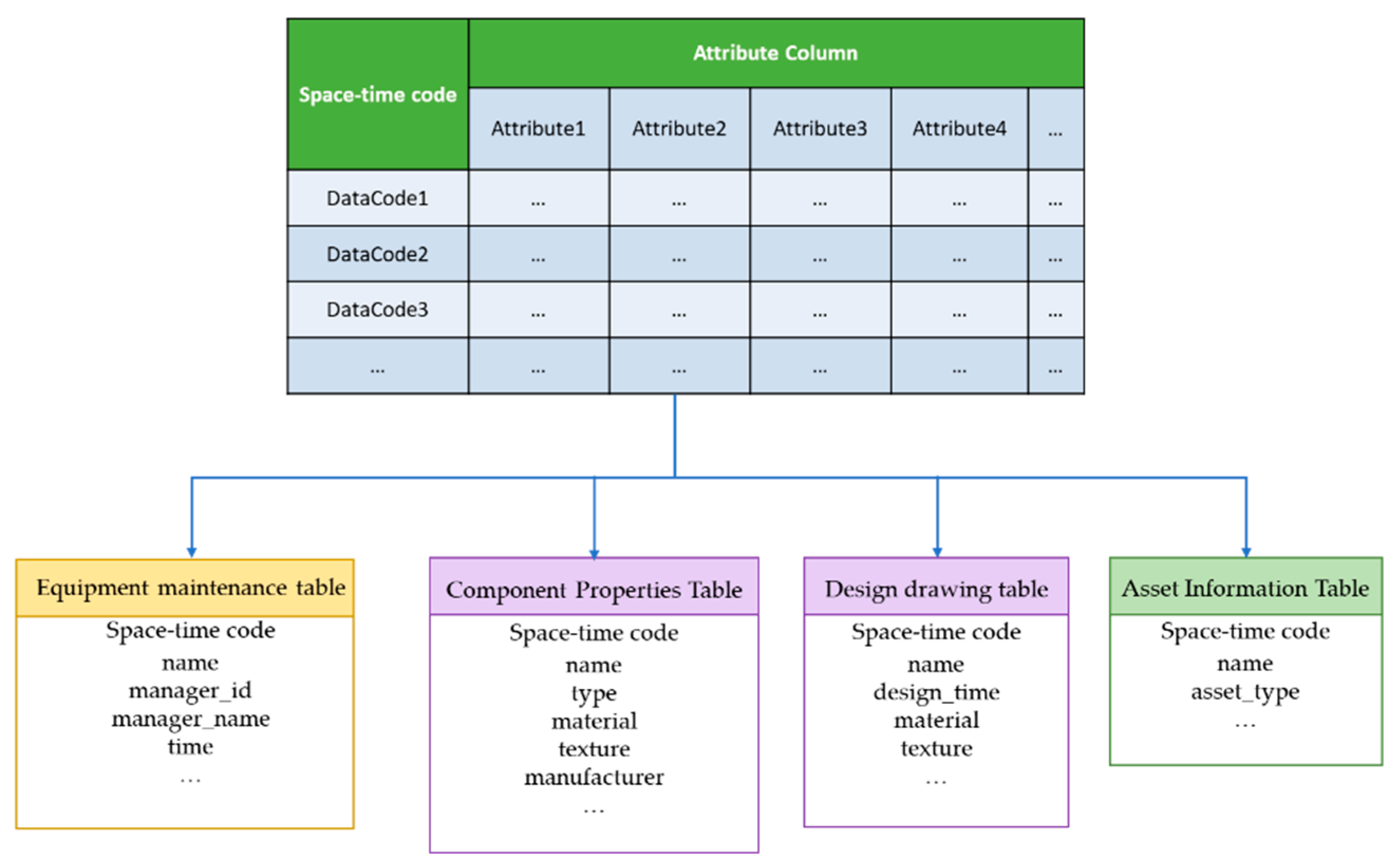
Using the indoor localization framework, multi-source data, such as various indoor object data, robot path data, and other data, can be divided into grid sets for expression. Trellis coding, therefore, can be used as a data index and an associative index. For the entire indoor space–time modeling, the large index table shown in

Table 1. Space–time index large table structure design.

Number	Column Name	Data Type	Description
1	$\mathrm{D}\mathrm{a}\mathrm{t}\mathrm{a}\mathrm{C}\mathrm{o}\mathrm{d}\mathrm{e}$	$\mathrm{V}\mathrm{a}\mathrm{r}\mathrm{c}\mathrm{h}\mathrm{a}\mathrm{r}\left(80\right)$	Space–time code
2	$\mathrm{T}\mathrm{y}\mathrm{p}\mathrm{e}\mathrm{I}\mathrm{D}$	$\mathrm{V}\mathrm{a}\mathrm{r}\mathrm{c}\mathrm{h}\mathrm{a}\mathrm{r}\left(2\right)$	Type code
3	StatusID	$\mathrm{V}\mathrm{a}\mathrm{r}\mathrm{c}\mathrm{h}\mathrm{a}\mathrm{r}\left(2\right)$	Equipment status code
4	$\mathrm{L}\mathrm{o}\mathrm{n}\mathrm{C}\mathrm{o}\mathrm{d}\mathrm{e}$	$\mathrm{V}\mathrm{a}\mathrm{r}\mathrm{c}\mathrm{h}\mathrm{a}\mathrm{r}\left(50\right)$	Longitude code
5	$\mathrm{L}\mathrm{a}\mathrm{t}\mathrm{C}\mathrm{o}\mathrm{d}\mathrm{e}$	$\mathrm{V}\mathrm{a}\mathrm{r}\mathrm{c}\mathrm{h}\mathrm{a}\mathrm{r}\left(50\right)$	Latitude code
6	$\mathrm{A}\mathrm{l}\mathrm{t}\mathrm{C}\mathrm{o}\mathrm{d}\mathrm{e}$	$\mathrm{V}\mathrm{a}\mathrm{r}\mathrm{c}\mathrm{h}\mathrm{a}\mathrm{r}\left(50\right)$	Elevation code
7	$\mathrm{C}\mathrm{o}\mathrm{m}\mathrm{p}\mathrm{o}\mathrm{n}\mathrm{e}\mathrm{n}\mathrm{t}\mathrm{N}\mathrm{a}\mathrm{m}\mathrm{e}$	$\mathrm{V}\mathrm{a}\mathrm{r}\mathrm{c}\mathrm{h}\mathrm{a}\mathrm{r}\left(15\right)$	Component name
8	$\mathrm{C}\mathrm{r}\mathrm{e}\mathrm{a}\mathrm{t}\mathrm{e}\mathrm{T}\mathrm{i}\mathrm{m}\mathrm{e}$	$\mathrm{C}\mathrm{h}\mathrm{a}\mathrm{r}\left(8\right)$	Creation time
9	$\mathrm{F}\mathrm{i}\mathrm{l}\mathrm{e}\mathrm{P}\mathrm{a}\mathrm{t}\mathrm{h}$	$\mathrm{V}\mathrm{a}\mathrm{r}\mathrm{c}\mathrm{h}\mathrm{a}\mathrm{r}\left(50\right)$	Data storage path

.

By the use of the table, the grid coding can be used as a foreign key to realize the mapping of indoor objects to space–time grids and the mapping of space–time grids to indoor objects, consequently realizing the unified management of indoor space–time, and the multi-source data can be efficiently associated, as shown in Figure 6.

4. Results

This section is mainly dedicated to the experiment of the indoor space–time grid model, consisting of two parts. The first part explains the experiment of local subdivision coding in space–time grid. This experiment verifies the feasibility and correctness of the coding and decoding algorithm of subdivision coding introduced above. The second part explains the indoor space–time grid modeling and organization visualization experiment, verifying the organization and integration ability of space–time grid for different indoor data from real data and simulation data.

4.1. Experiments on Localized Encoding and Decoding in Space–Time Grids

This section is mainly about the experiments of local spatial subdivision coding and local time coding in the spatiotemporal grid. More specifically, the experiments involve the encoding and decoding of local spatial subdivision coding and the coding and decoding of local time coding. Experiments prove the correctness and feasibility of the indoor local segmentation framework and the above algorithms. The experimental data are spatiotemporal data generated randomly by uniform distribution to satisfy the local spatial profile spatial extent requirement and to satisfy the local temporal coding time requirement.

In this experiment, five groups of random space–time simulation data are randomly generated. Then, the simulation data are encoded and decoded from the perspective of space and time. One must check whether the decoded grid contains random points before encoding and whether the time–space domain after encoding and decoding contains time points before encoding. Next, one must verify that the codec correctly expresses the local coordinate information and time information of the original data. In the spatial coding experiment, the 10th level and the 15th level of the partial dissection level were used to conduct experiments on the simulation data. In the time coding experiment, the 20th level and the 26th level of the local time dissection level were used to conduct experiments on the simulation data. The results are shown in

Table 2. Sectioning level and time domain relationship table.

Quantity	level	Encoding Time	Decoding Time	Correct Rate
1000	10	1.05 ms	0.95 ms	100%
5000	10	3.97 ms	2.99 ms	100%
10,000	10	8.05 ms	6.98 ms	100%
50,000	10	37.92 ms	50.93 ms	100%
100,000	10	88.78 ms	91.23 ms	100%
1000	15	1.99 ms	2.01 ms	100%
5000	15	5.01 ms	7.95 ms	100%
10,000	15	15.93 ms	14.96 ms	100%
50,000	15	52.03 ms	60.73 ms	100%
100,000	15	107.7 ms	99.86 ms	100%
1000	20	0.99 ms	1.03 ms	100%
5000	20	2.98 ms	7.02 ms	100%
10000	20	5.98 ms	12.97 ms	100%
50,000	20	28.95 ms	64.81 ms	100%
100,000	20	61.09 ms	143.95 ms	100%
1000	26	1.01 ms	1.02 ms	100%
5000	26	3.05 ms	7.01 ms	100%
10,000	26	6.02 ms	13.94 ms	100%
50,000	26	31.93 ms	64.92 ms	100%
100,000	26	60.86 ms	144.61 ms	100%

.

4.2. Indoor Space–Time Grid Modeling and Tissue Visualization Experiments

This experiment is to verify the spatial organization ability of the indoor space–time grid for multiple indoor spaces.

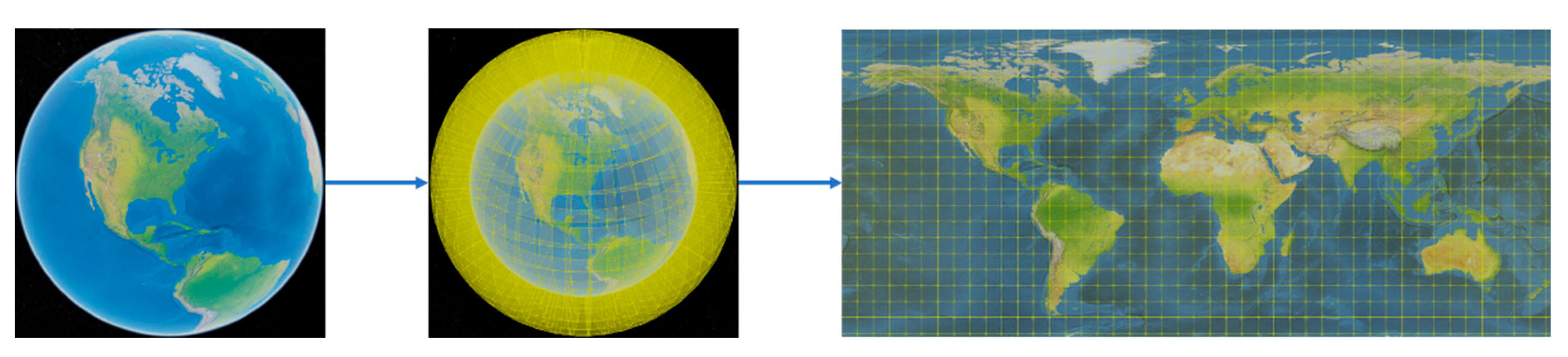
First, realize the BeiDou Grid Digital Earth. A 3D digital Earth is constructed through the Cesium platform. The Earth space is then decomposed into a multi-scale nested spatial 3D grid system based on the BeiDou grid technology to achieve a grid dissection of the Earth, as shown in Figure 7.

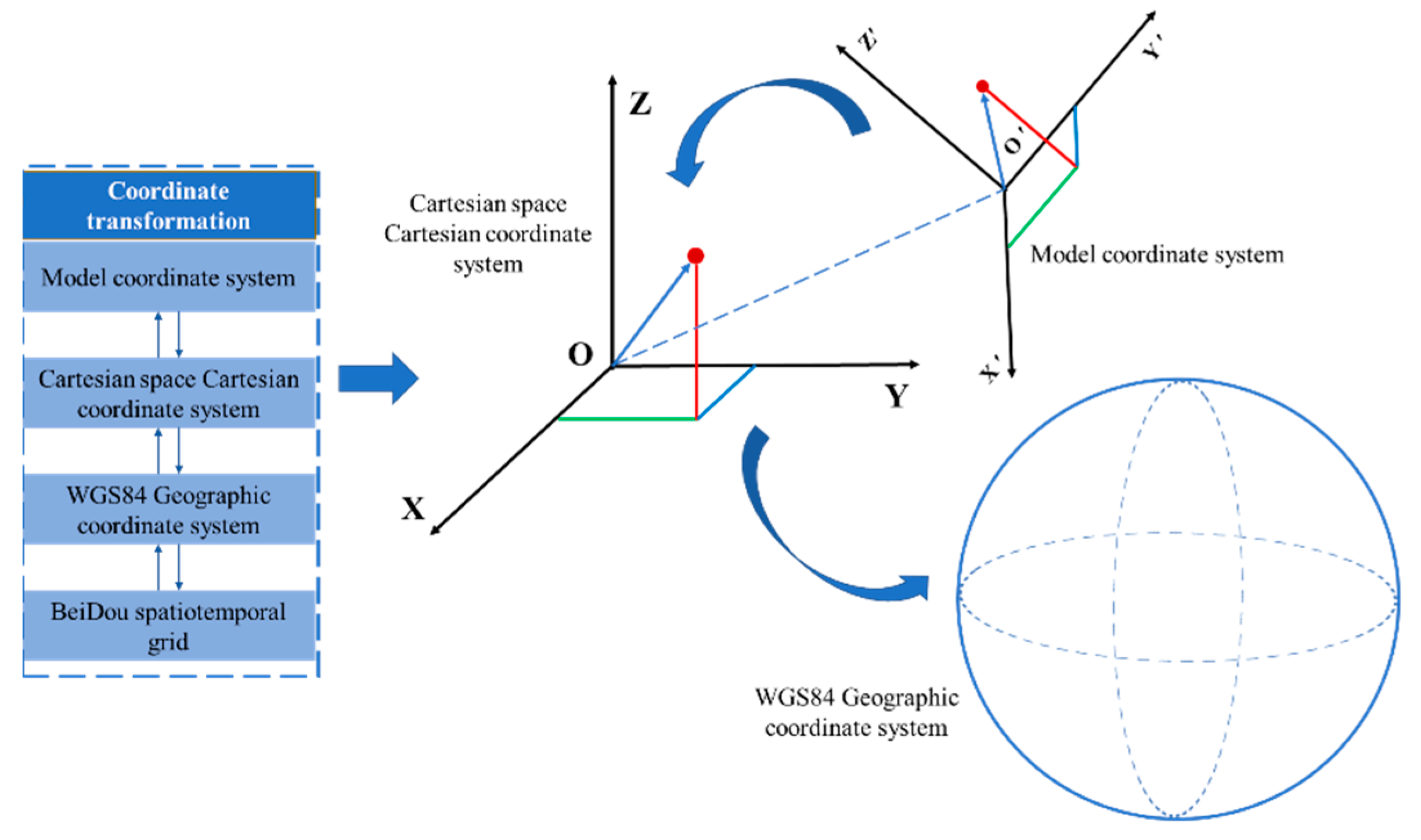
The experimental data used in this paper are the BIM model of Guanlan Commercial Street in Baiyin City. To establish a link between the BIM model and the BeiDou grid, a coordinate transformation is required to enable the grid to associate data in the BIM model. Coordinate conversion refers to the transformation of model object data into grid space location and grid space attributes. In the process of converting the grid space location, it involves the conversion of the central coordinate system where the original model is located, the Earth’s Cartesian coordinate system, and the coordinate conversion between WGS84 geographic coordinate system and BeiDou grid code, as shown in Figure 8.

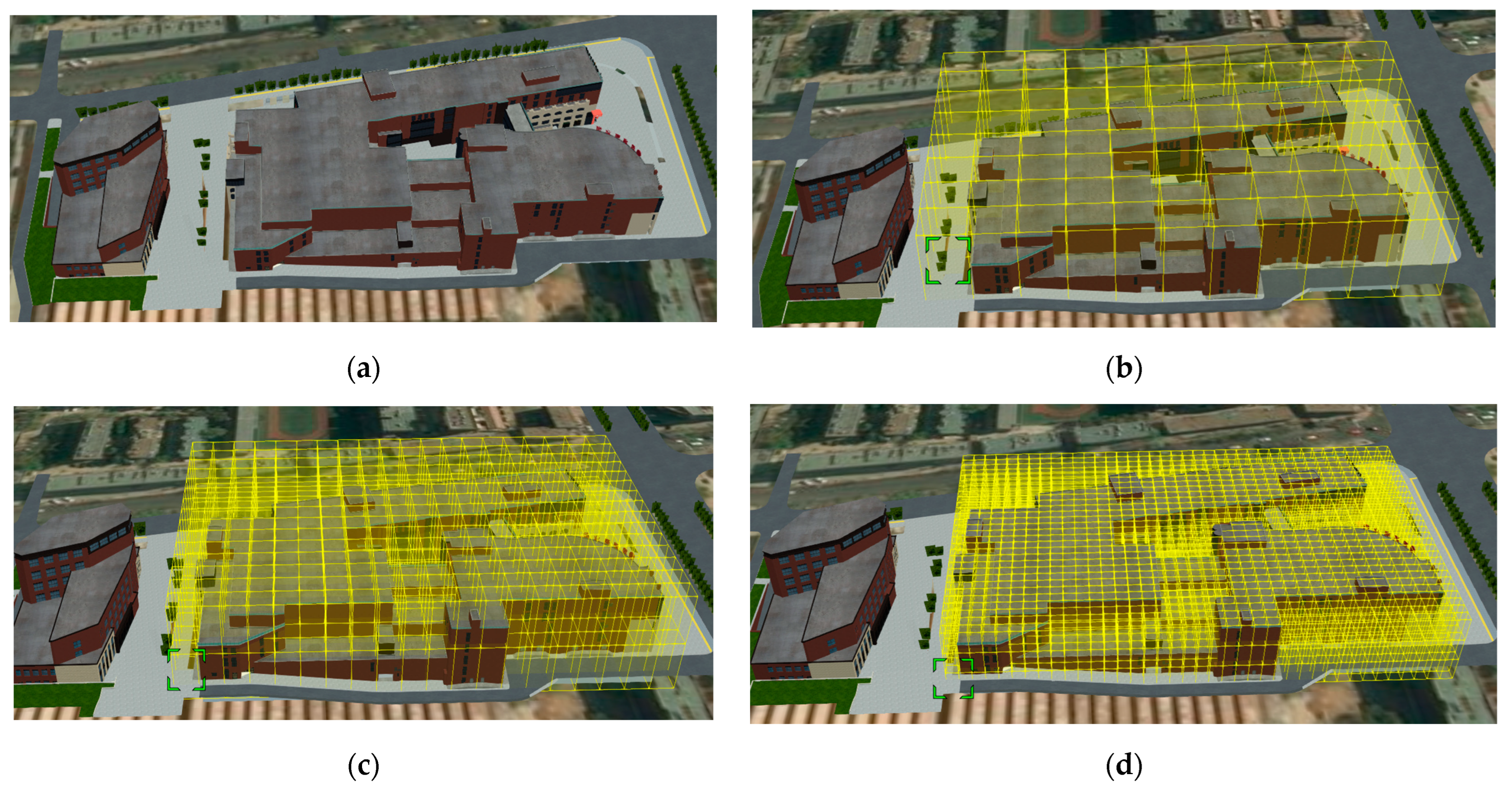
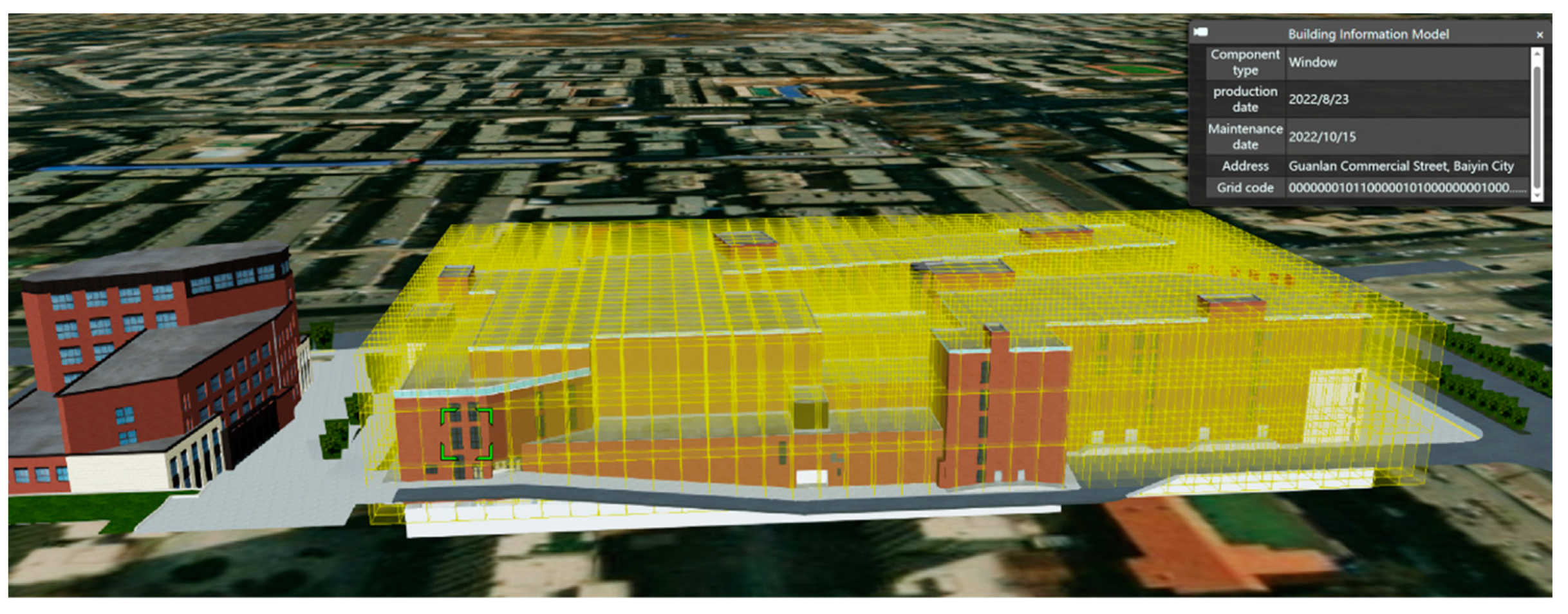
Therefore, its visual spatio-time grid coding at different levels is shown in Figure 9. Taking the spatiotemporal grid code as the row key and various types of data as the column attributes, the grid is used as a data container for correlation and querying to realize the information fusion of different data in the room. The result of the grid association query is shown in Figure 10.

5. Discussion

Through the above experimental results, the following conclusions can be drawn:

• From the experimental results shown in Table 2, it can be concluded that in the spatial encoding and decoding, when the level increases, the time consumption increases slightly, and each encoding and decoding takes about 1 microsecond. In temporal encoding and decoding, when the level becomes larger, the time consumption is almost unchanged, and the encoding operation is faster than the decoding operation. When comparing these two processes, the encoding operation takes about 0.6 microseconds each time, and the decoding operation takes about 1.4 microseconds each time. The time and space encoding and decoding algorithms take seconds under millions of operations. The experiment also proves that the temporal encoding and decoding algorithms and spatial encoding and decoding algorithms proposed in this paper are correct.
• From the experimental results shown in Figure 9 and Figure 10, it can be concluded that under the indoor space–time grid modeling method, local indoor space can be modeled locally. At the same time, by using the global coordinate origin of the local coordinate system itself, the global unification of different indoor local coordinate systems can be realized, making the integration of all indoor spaces possible. In this way, in the future, not only can one map be used to manage all indoor spaces, but it can also be combined with the existing outdoor space modeling methods based on the Beidou framework to achieve unified indoor and outdoor data management.

In summary, from the analysis of the experimental results, it can be concluded that the indoor time-varying spatial grid model proposed in this paper is feasible and correct. This model is of great significance to realize the integration of indoor and outdoor space. By using the spatiotemporal grid code as the row key and various types of data as the column attributes, the indexed large table is established to realize the information fusion of different data in the room. In other words, the spatiotemporal grid is used as a data container to achieve data organization and integration. At the same time, the grid is naturally suitable for the operation of all kinds of indoor path planning algorithms. For example, indoor fire emergency rescue and indoor mobile robots in real-time accurate path planning.

6. Conclusions

In this paper, an indoor spatiotemporal grid coding modeling method is proposed. This method is based on the research background of spatiotemporal modeling in an indoor environment with more time-varying space, the process of analyzing the characteristics of indoor environment and existing indoor modeling methods, the indoor space–time grid modeling method for global subdivision, indoor local space subdivision, and local time subdivision. Based on the Beidou subdivision framework, a set of local subdivision frameworks suitable for indoors is proposed under the Beidou global subdivision grid, and then a local time encoding model is proposed on the basis of the time encoding model. The indoor local space subdivision and local time coding model are combined to realize indoor space–time grid modeling. At the same time, a set of data storage methods, based on space–time grid, is designed so that the space–time model can carry multi-source heterogeneous data. When the physical state of the real object changes, the object information in the space–time model can be dynamically updated, making it perfectly compatible with the time-varying characteristics of indoor space.

Although some research results have been achieved in this paper, there are still some problems that need to be improved and optimized. For example, in the future, it is necessary to provide more types of data space–time grid expression methods to further improve the expression of the indoor space–time environment.

References

- Li, B.; Duan, Z. Visual odometer based on deep learning in dynamic indoor environment. J. Chin. Comput. Syst. 2023, 44, 49. [Google Scholar]
- Lucattini, L.; Poma, G.; Covaci, A.; de Boer, J.; Lamoree, M.H.; Leonards, P.E.G. A review of semi-volatile organic compounds (SVOCs) in the indoor environment: Occurrence in consumer products, indoor air and dust. Chemosphere 2018, 201, 466–482. [Google Scholar] [CrossRef] [PubMed]
- Liu, H.; Zhang, Z.; Zhu, Y.; Zhu, S.C. Self-supervised incremental learning for sound source localization in complex indoor environment. In Proceedings of the 2019 International Conference on Robotics and Automation, Montreal, QC, Canada, 20–24 May 2019. [Google Scholar]
- Savva, M.; Chang, A.X.; Dosovitskiy, A.; Funkhouser, T.; Koltun, V. MINOS: Multimodal indoor simulator for navigation in complex environments. arXiv 2017, arXiv:1712.03931. [Google Scholar]
- Feng, Z.; Yu, C.W.; Cao, S.J. Fast prediction for indoor environment: Models assessment. Indoor Built Environ. 2019, 28, 727–730. [Google Scholar] [CrossRef] [Green Version]
- Kashiwagi, I.; Taga, T.; Imai, T. Time-varying path-shadowing model for indoor populated environments. IEEE Trans. Veh. Technol. 2009, 59, 16–28. [Google Scholar] [CrossRef]
- Hu, X.G.; Cheng, C.Q.; Tong, X.C. Research on 3D data representation based on GeoSOT-3D. J. Peking Univ. 2015, 51, 1022–1028. [Google Scholar]
- Sun, Z.Q.; Cheng, C.Q. True 3D Data Expression Based on GeoSOT-3D Ellipsoid Subdivision. Geomat. World 2016, 23, 40–46. [Google Scholar]
- Wang, L. Research on Time Subdivision Code Model. PhD Thesis, Peking University, Beijing, China, 2016. [Google Scholar]
- Diakité, A.A.; Zlatanova, S. Spatial subdivision of complex indoor environments for 3D indoor navigation. Int. J. Geogr. Inf. Sci. IJGIS 2018, 32, 213–235. [Google Scholar] [CrossRef] [Green Version]
- Chen, W.; Guan, M.; Wang, L.; Ruby, R.; Wu, K. FLoc: Device-free passive indoor localization in complex environments. In Proceedings of the 2017 IEEE International Conference on Communications, Paris, France, 21–25 May 2017. [Google Scholar]
- Yan, L.Y. Research on Path Planning Technology of Mobile Car in Indoor Dynamic Environment. Master’s Thesis, Southeast University, Nanjing, China, 2018. [Google Scholar]
- He, Y.F. Research on Path Planning Algorithm of Indoor Micro UAV. Master’s Thesis, Nanjing University of Aeronautics and Astronautics, Nanjing, China, 2014. [Google Scholar]
- Jin, L.S.; Guo, L.; Wang, R.B.; Zhang, R.H.; Li, H.L. System design and navigation control for vision based CyberCar. In Proceedings of the 2006 IEEE International Conference on Vehicular Electronics and Safety, Shanghai, China, 13–15 December 2006. [Google Scholar]
- Liu, Y.; Wang, H.; Xie, J. Global path planning method based on geometry algorithm in a strait environment. In Proceedings of the 2010 International Conference on Electrical and Control Engineering, Wuhan, China, 25–27 June 2010. [Google Scholar]
- Del Pero, L.; Bowdish, J.; Fried, D.; Kermgard, B.; Hartley, E.; Barnard, K. Bayesian geometric modeling of indoor scenes. In Proceedings of the 2012 IEEE Conference on Computer Vision and Pattern Recognition, Providence, RI, USA, 16–21 June 2012. [Google Scholar]
- Oesau, S. Geometric Modeling of Indoor Scenes from Acquired Point Data. Ph.D. Thesis, University Nice Sophia Antipolis, Nice, France, 2015. [Google Scholar]
- Chen, K.; Lai, Y.K.; Hu, S.M. 3D indoor scene modeling from RGB-D data: A survey. Comput. Vis. Media 2015, 1, 267–278. [Google Scholar] [CrossRef] [Green Version]
- Ikehata, S.; Yang, H.; Furukawa, Y. Structured indoor modeling. In Proceedings of the IEEE International Conference on Computer Vision, Washington, DC, USA, 7–13 December 2015. [Google Scholar]
- Hong, S.; Jung, J.; Kim, S.; Cho, H.; Lee, J.; Heo, J. Semi-automated approach to indoor mapping for 3D as-built building information modeling. Comput. Environ. Urban Syst. 2015, 51, 34–46. [Google Scholar] [CrossRef]
- Zhou, X.; Xie, Q.; Guo, M.; Zhao, J.; Wang, J. Accurate and efficient indoor pathfinding based on building information modeling data. IEEE Trans. Ind. Inform. 2020, 16, 7459–7468. [Google Scholar] [CrossRef]
- Jamali, A.; Abdul Rahman, A.; Boguslawski, P.; Kumar, P.; Gold, C.M. An automated 3D modeling of topological indoor navigation network. GeoJournal 2017, 82, 157–170. [Google Scholar] [CrossRef] [Green Version]
- Pintore, G.; Mura, C.; Ganovelli, F.; Fuentes-Perez, L.; Pajarola, R.; Gobbetti, E. State-of-the-art in automatic 3D reconstruction of structured indoor environments. Comput. Graph. Forum 2020, 39, 667–699. [Google Scholar] [CrossRef]
- Plutniak, S. The strength of parthood ties. Modelling spatial units and fragmented objects with the TSAR method—Topological Study of Archaeological Refitting. J. Archaeol. Sci. 2021, 136, 105501. [Google Scholar] [CrossRef]
- Zhu, J.; Li, Q.; Cao, R.; Sun, K.; Liu, T.; Garibaldi, J.M.; Qiu, G. Indoor topological localization using a visual landmark sequence. Remote Sens. 2019, 11, 73. [Google Scholar] [CrossRef] [Green Version]
- Tran, H.; Khoshelham, K.; Kealy, A.; Díaz-Vilariño, L. Extracting topological relations between indoor spaces from point clouds. ISPRS Ann. Photogramm. Remote Sens. Spat. Inf. Sci. 2017, 4, 401. [Google Scholar] [CrossRef] [Green Version]
- Rituerto, A.; Murillo, A.C.; Guerrero, J.J. Semantic labeling for indoor topological mapping using a wearable catadioptric system. Robot. Auton. Syst. 2014, 62, 685–695. [Google Scholar] [CrossRef]
- Lin, W.Y.; Lin, P.H. Intelligent generation of indoor topology (i-GIT) for human indoor pathfinding based on IFC models and 3D GIS technology. Autom. Constr. 2018, 94, 340–359. [Google Scholar] [CrossRef]
- Heng, L.; Lee, G.H.; Fraundorfer, F.; Pollefeys, M. Real-time photo-realistic 3d mapping for micro aerial vehicles. In Proceedings of the 2011 IEEE/RSJ International Conference on Intelligent Robots and Systems, San Francisco, CA, USA, 25–30 September 2011. [Google Scholar]
- Gorte, B.; Zlatanova, S.; Fadli, F. Navigation in Indoor Voxel Models. ISPRS Annals of the Photogrammetry. Remote Sens. Spat. Inf. Sci. 2019, 4, 279–283. [Google Scholar]
- Chandel, V.; Ahmed, N.; Arora, S.; Ghose, A. InLoc: An end-to-end robust indoor localization and routing solution using mobile phones and BLE beacons. In Proceedings of the 2016 International Conference on Indoor Positioning and Indoor Navigation, Alcala de Henares, Spain, 4–7 October 2016. [Google Scholar]
- Zhu, J.; Durgin, G.D. Indoor/outdoor location of cellular handsets based on received signal strength. In Proceedings of the 2005 IEEE 61st Vehicular Technology Conference, Stockholm, Sweden, 30 May–1 June 2005. [Google Scholar]
- Cheng, C.Q. An Introduce to Spatial Information Subdivision Organization; Science Press: Beijing, China, 2012. [Google Scholar]
- Zhai, W.X. Unmanned Aircraft Vehicle Neighbourhood Location Grid Computing Model. Ph.D. Thesis, Peking University, Beijing, China, 2018. [Google Scholar]
- Zhang, H.; Li, G. Precise Indoor Path Planning Based on Hybrid Model of GeoSOT and BIM. ISPRS Int. J. Geo-Inf. 2022, 11, 243. [Google Scholar] [CrossRef]
- Tong, X.C.; Wang, L.; Wang, R.; Lai, G.L.; Ding, L. An Efficient Integer Coding and Computing Method for Multiscale Time Segment. Acta Geod. Cartogr. Sin. 2016, 45, 66–76. [Google Scholar]
Figure 1.
Beidou grid model. (a) The three virtual extensions of Beidou grid; (b) Beidou section hierarchy.
Figure 2.
The seven virtual extensions of time.
Figure 3.
The levels of indoor partial division.
Figure 4.
Schematic diagram of indoor local grid coding.
Figure 5.
The levels of indoor time division.
Figure 6.
Indoor space–time grid data table.
Figure 7.
Beidou global grid display.
Figure 8.
Coordinate conversion.
Figure 9.
Visualization display of different levels of coding. (a) original data; (b) 22 level; (c) 23 level; (d) 24 level.
Figure 10.
Correlation query display.