Article

Simulation and Driving Factor Analysis of Satellite-Observed Terrestrial Water Storage Anomaly in the Pearl River Basin Using Deep Learning

1
School of Civil Engineering, Sun Yat-Sen University, Guangzhou 510275, China
2
School of Computer Science and Engineering, Sun Yat-Sen University, Guangzhou 510275, China
3
School of Atmospheric Science, Sun Yat-Sen University, Guangzhou 510275, China
4
School of Software Engineering, Sun Yat-Sen University, Guangzhou 510275, China
*
Author to whom correspondence should be addressed.
These authors contributed equally to this work.
Remote Sens. 2023, 15(16), 3983; https://doi.org/10.3390/rs15163983
Submission received: 14 July 2023 / Revised: 4 August 2023 / Accepted: 9 August 2023 / Published: 11 August 2023
(This article belongs to the Section Environmental Remote Sensing)

Abstract

:
Accurate estimation of terrestrial water storage (TWS) and understanding its driving factors are crucial for effective hydrological assessment and water resource management. The launches of the Gravity Recovery and Climate Experiment (GRACE) satellites and their successor, GRACE Follow-On (GRACE-FO), combined with deep learning algorithms, have opened new avenues for such investigations. In this study, we employed a long short-term memory (LSTM) neural network model to simulate TWS anomaly (TWSA) in the Pearl River Basin (PRB) from 2003 to 2020, using precipitation, temperature, runoff, evapotranspiration, and leaf area index (LAI) data. The performance of the LSTM model was rigorously evaluated, achieving a high average correlation coefficient (r) of 0.967 and an average Nash–Sutcliffe efficiency (NSE) coefficient of 0.912 on the testing set. To unravel the relative importance of each driving factor and assess the impact of different lead times, we employed the SHapley Additive exPlanations (SHAP) method. Our results revealed that precipitation exerted the most significant influence on TWSA in the PRB, with a one-month lead time exhibiting the greatest impact. Evapotranspiration, runoff, temperature, and LAI also played important roles, with interactive effects among these factors. Moreover, we observed an accumulation effect of precipitation and evapotranspiration on TWSA, particularly with shorter lead times. Overall, the SHAP method provides an alternative approach for the quantitative analysis of natural driving factors at the basin scale, shedding light on the natural dominant influences on TWSA in the PRB. The combination of satellite observations and deep learning techniques holds promise for advancing our understanding of TWS dynamics and enhancing water resource management strategies.

1. Introduction

Terrestrial water storage (TWS) refers to the total amount of water stored on or within the land surface, mainly including surface runoff, soil moisture, groundwater, snow, and water in lakes and reservoirs. It serves as a comprehensive indicator of the global hydrological cycle [1] and plays an important role in measuring water resource availability [2]. Furthermore, TWS reflects vegetation growth [3], climate change [4], and drought [5]. With an increasing water demand and the more frequent occurrence of drought and flood disasters under climate change [6], investigating the major drivers of TWS and quantifying their relative contributions within the Pearl River Basin (PRB) are essential for understanding extreme hydrological disasters, food security, and water resource management in the PRB [7].
The analysis of driving factors has been challenging in the past due to the difficulty in obtaining TWS measurements with high accuracy. Recently, a number of other optical and microwave-based satellite remote sensing techniques have been proposed to detect individual components of terrestrial water reserves. For example, Soil Moisture Active and Passive (SMAP) satellites and Fengyun-3 satellites are used to monitor soil water, Water Cycle Observation Mission (WCOM) satellites are used to detect snow water content, Google Earth Engine (GEE) is used to detect water volume change information, and Surface Water and Ocean Topography (SWOT) microsensors are used to monitor surface and groundwater. The launches of the Gravity Recovery and Climate Experiment (GRACE) satellites in 2002 and the GRACE Follow-On (GRACE-FO) in 2018 have revolutionized our ability to understand and monitor global water resources. Unlike other satellite sensor products, GRACE, which utilizes remote sensing technology, has delivered invaluable and highly accurate observations of the global total water storage anomalies with all components [8], enabling us to assess changes in water availability on a large scale. GRACE’s data have been instrumental in studying hydrological processes, tracking water availability, detecting droughts, and understanding the impacts of climate change on water resources. Its contributions have significantly advanced our knowledge and have become a cornerstone for effective water resource management strategies worldwide.
Various approaches have been employed to analyze the driving factors of TWS anomaly (TWSA), including land surface models, hydrological models, and statistical analysis. Pokhrel et al. [6] used ensemble hydrological simulations and found that the projected changes in global TWS are driven primarily by climate forcing rather than land and water management activities. Deng et al. [9] calculated the climate resilience coefficient to analyze the impact of climate factors on hydrological systems and concluded that in the process of water storage reduction in 2012, potential evapotranspiration accounted for 90%, precipitation accounted for 7%, and surface properties accounted for 3%. But due to the uncertainty of the climate forcing data and the absence of relevant process modules (e.g., human activity and vegetation dynamics), TWS simulated by land surface models and hydrological models—only a subset of TWS components—often does not match the data observed by GRACE [5,6]. Additionally, the PRB exhibits a highly heterogeneous geological environment and intense human activities. These factors pose significant challenges for accurately estimating TWS using hydrological models [5,10,11]. Furthermore, as the driving factors are interdependent, solely relying on linear relationships to investigate the primary driving factors of TWS may lead to misleading results.
Fortunately, the rapid advancement of deep learning techniques provides a viable solution to the aforementioned challenges in hydrology and related fields [12,13,14,15]. Deep learning modeling, a nonparametric technique, proves effective in approximating the intricate nonlinear relationship between input and output variables, devoid of any prior assumptions regarding the underlying physical system [16,17,18]. In fact, deep learning models have gained widespread adoption in hydrological research. On the one hand, these models are used to improve the simulation and prediction of hydrological variables, thereby improving the quality of data products [19,20,21]. On the other hand, they are gradually being used for hydrological process understanding and data mining [22,23,24,25]. Among the various deep learning models, the LSTM model has been well used in hydrological time series simulation and forecasting research, including flood forecasting, water temperature forecasting, and soil water data extension [17,19,24]. Further, explainable machine learning methods have been developed to elucidate patterns captured by machine learning and deep learning models. Techniques such as accumulated local effects (ALE) [22], global to local analysis (local interpretable model-agnostic explanations, LIME) [26,27], and SHapley Additive exPlanations (SHAP) techniques [28,29] have been widely used in the field of hydrology and meteorology. Particularly, the SHAP method is a novel explainable machine learning method that provides an intuitive understanding of the relationship between the model’s input variables and the predicted results [30,31].
So far, there have been a large number of studies using deep learning models to reconstruct TWSA sequences and achieve favorable results [1,18,32]. However, few studies have focused on the driving factor analysis of TWS with deep learning methods. Some studies have applied soil moisture, which is a component of TWS and highly correlated with TWS, as an input factor for models to achieve better simulation results, which hinders the examination of causal relationships among drivers. In this study, we avoid using direct TWS components as input factors. The SHAP method is combined with an LSTM model to uncover patterns of TWS captured by the LSTM network.
Therefore, the primary objectives of this study are as follows: (1) Employ GRACE data, meteorological data, and underlying surface data to train an LSTM model for simulating the dynamics of TWS in the PRB and evaluate its performance; (2) quantify the relative importance of driving factors of TWS in the PRB using an explainable machine learning framework; and (3) analyze the influencing mechanism of TWS driving factors in the PRB.

2. Materials and Methods

2.1. Study Area

The PRB encompasses a geographical area between the longitudes 102°14′E–115°53′E and the latitudes 21°31′N–26°49′N (Figure 1). With a basin area of about 450,000 km2 and an annual water discharge of 3.36 × 10¹¹ m3, the Pearl River is China’s second largest river by discharge volume and third largest river in terms of basin area [33]. The PRB stretches across the Yunnan–Guizhou Plateau and the Guangdong–Guangxi Hills, primarily situated in the subtropical and tropical monsoon climate regions characterized by diverse landscapes and abundant precipitation. Notably, from April to September, precipitation during these months accounts for 80% of the total annual precipitation [34]. The Pearl River Delta region is densely populated, exhibits high water consumption, and experiences frequent droughts and floods [35,36].

2.2. Data Sources

2.2.1. GRACE Data

The GRACE data used in this study were obtained from the NASA Goddard Space Flight Center (GSFC). The estimation of TWS was derived using the mass concentration blocks (mascons) method [37]. This method facilitates the implementation of geophysical constraints and effectively filters noise from GRACE/GRACE-FO observations, providing a more rigorous alternative to the standard spherical harmonic method [38]. The TWSA values in this data product are relative to the average from 2004 to 2010, with a spatial resolution of 0.5° and a temporal resolution of one month. Our analysis focuses on data spanning from April 2002 to December 2020. However, due to technical issues with satellite equipment, there are gaps in the data for several months, and these periods of missing data are directly excluded from the analysis.

2.2.2. Input Data

In this study, the analysis of driving factors was carried out by excluding TWS components such as soil moisture to ensure the integrity of the analysis. However, it is worth noting that explainable machine learning methods are most effective when the model’s performance is satisfactory [39]. Therefore, to ensure the performance of the LSTM model and the validity of the driving factor analysis, five driving factors including precipitation, evapotranspiration, temperature, runoff, and LAI were considered as input features.
The precipitation and mean temperature data used in this study were obtained from the widely used Climate Research Unit (CRU) Time Series Climate dataset, specifically version 4.03, released by the University of East Anglia. This dataset employs an angle–distance weighting method to interpolate in situ climate data [40]. It provides a spatial resolution of 0.5° and a monthly temporal resolution. Additionally, the monthly actual evapotranspiration (AET) data were extracted from the Global Land Evaporation Amsterdam Model (GLEAM), which incorporates satellite observations of climate and environmental variables [41,42].
Furthermore, the influence of runoff and leaf area index (LAI) was taken into account in this study. Since we needed gridded format data, which are not available for runoff from in situ measurement, we utilized the European Centre for Medium-range Weather Forecasts ReAnalysis 5-Land (ERA5-Land) reanalysis dataset, which provides assimilated runoff data. This dataset combines model data with global observations and is considered one of the most state-of-the-art datasets in land surface applications. It has a spatial resolution of 0.25° and a monthly temporal resolution.
LAI data can be downloaded from the Land-Atmosphere Interaction Research Group at Sun Yat-sen University (SYSU). This dataset is an improved version derived from the post-processing of the MODerate-resolution Imaging Spectroradiometer (MODIS) version 6 LAI product. It utilizes a two-step integration method, resulting in enhanced data quality compared to the raw MODIS data [43,44]. This ensures a continuous and consistent dataset for analysis [44]. The LAI dataset has a spatial resolution of 0.5° and a temporal resolution of monthly intervals.
This study selected the above data from April 2002 to December 2020 in the PRB. To ensure consistency, the data were unified into the grid of the GRACE data with the nearest neighbor interpolation method. More details are listed in Table 1.

2.3. Methods

2.3.1. LSTM Model

We used LSTM models (Figure 2b) to simulate the TWSA dynamics at the setting time scale in this study. As a special recurrent neural network (RNN), LSTM is a typical sequence learning model [45]. Its notable advantage lies in its ability to capture information from distant time steps, effectively addressing the challenge of vanishing gradients commonly encountered in standard RNNs. This is achieved through LSTM’s incorporation of two types of states and a specialized gated structure (Figure 2a). During the training process, the RNN updates the weights in the recurrent unit through the backpropagation-through-time algorithm [46,47]. When the sequence is long, the weight-updated signal decays rapidly during propagation along the chain, preventing the model from learning information from distant time steps. This phenomenon is known as vanishing gradients.
Under the premise of considering the effect of the model and applying the explainable machine learning method, we designed the model for this study as shown in Figure 2b. The model architecture consists of an input layer, an LSTM layer, a hidden layer, and an output layer. The LSTM layer and the dense layer have 256 neurons each, while the output layer has 1 neuron. To ensure that each simulation of the TWSA value incorporates information of the same length, we utilized only the output from the last time step of the LSTM layer. We then mapped the output from 256 hidden cells to 1 output cell through the fully connected layer.
Previous studies have shown that there is a time lag of one to two months between climate forcing data and the TWSA observed by GRACE satellites [46]. At the same time, in order to verify whether the LSTM model can effectively capture information from the previous time step, we set the LSTM time step to 11, that is, the precipitation, air temperature, evapotranspiration, runoff, and LAI in the current month and the simulated values from the preceding 10 months were used as input series to simulate the TWSA of the current month (Figure 2c). The model can be expressed by the following formula:
y t = f x t ,   x t 1 ,   , x t 10
where y t refers to the simulation of TWSA in month t ; x t refers to the input variable in month t ; x t 1 ,   ,     x t 10 is the input vector for the corresponding months from t 1 to t 10 .
To fetch the best model, we employed a strategy to increase the number of samples by treating each time grid point in the basin as an individual sample. We utilized the five-fold cross-validation method to train the models and select the optimal one. The dataset was divided evenly into five consecutive folds in periods from 2002 to 2020 (Table 2). During each iteration, one of the five folds was designated as the testing set, while the remaining four folds were used to train the model. This process resulted in the generation of five different models. For each model, we used the Adam optimization algorithm [48] to continuously update the model parameters to gradually reduce the root mean square error of the TWSA simulated values and the observed values of the training set. When the Nash–Sutcliffe efficiency (NSE) coefficient between the simulated values and the observed values of TWSA of the testing set no longer grew, the model corresponding to the maximum NSE coefficient was chosen as the model of the experiment in this group. To prevent overfitting, we applied dropout regularization [49] with an empirical setting of 0.5. Finally, we reconstructed the TWSA sequences from 2002 to 2020 using five different models and utilized the best model to analyze TWSA’s response to precipitation, temperature, evapotranspiration, runoff, and vegetation.

2.3.2. Model Evaluation Metrics

In this study, the correlation coefficient (r), normalized root mean square error (NRMSE), NSE, and bias are used to evaluate the simulation performance of the model. These evaluation indices can be calculated using the following formulas:
r = i = 1 n y s i y s i ¯ y o i y o i ¯ i = 1 n y s i y s i ¯ 2 × i = 1 n y o i y o i ¯ 2  
N R M S E = i = 1 n y s i y o i 2 i = 1 n y o i 2  
N S E = 1 i = 1 n y s i y o i 2 i = 1 n y o i y o i ¯ 2  
b i a s = i = 1 n y s i y o i i = 1 n y o i  
where n denotes the number of samples; y s i , y o i are the simulated values and GRACE observed values, respectively. The closer the bias and NRMSE are to 0, the better the model performance, and the closer the correlation coefficient and the NSE are to 1, the better the model performance.

2.3.3. Interpretation Methods

SHAP is a game theory-based machine learning interpretation technique that unifies common additive feature attribution methods with better computational performance and better alignment with human intuition [30,50].
Additive feature attribution methods assign an effect ϕ i to each feature, and by summing the effects of all feature attributions, we can approximate the output f x of the original model. The process can be expressed using the following formula:
f x = g x = ϕ 0 + i = 1 M ϕ i x i  
ϕ i = S N / i S ! M S 1 ! M ! f x S i f x S  
where x 0 ,   1 M , M is the number of simplified input features, S is the set of nonzero indexes, and ϕ i R ; f x is the output of the original model; h x is a mapping function which explanation models used to turn original inputs x into simplified inputs x through x = h x x ; the explanation model function g x matches the original model f x when x = h x x ; ϕ 0 = f h x 0 represents the model output with all simplified inputs toggled off.
SHAP values serve as a comprehensive measure of feature importance and provide a solution to Equation (7). They represent the Shapley values of a conditional expectation function of the original model. The SHAP values indicate the changes in the model’s predicted values when considering a specific feature. They explain how the features contribute to the predicted values compared to the baseline value without any feature.
DeepSHAP is a computational method designed to approximate the SHAP values efficiently. It is an improvement on the traditional additive interpretation method called Deeplift [30]. In this study, DeepSHAP was employed to reveal the impact of driving factors at different time steps and quantify their individual contributions.

3. Results

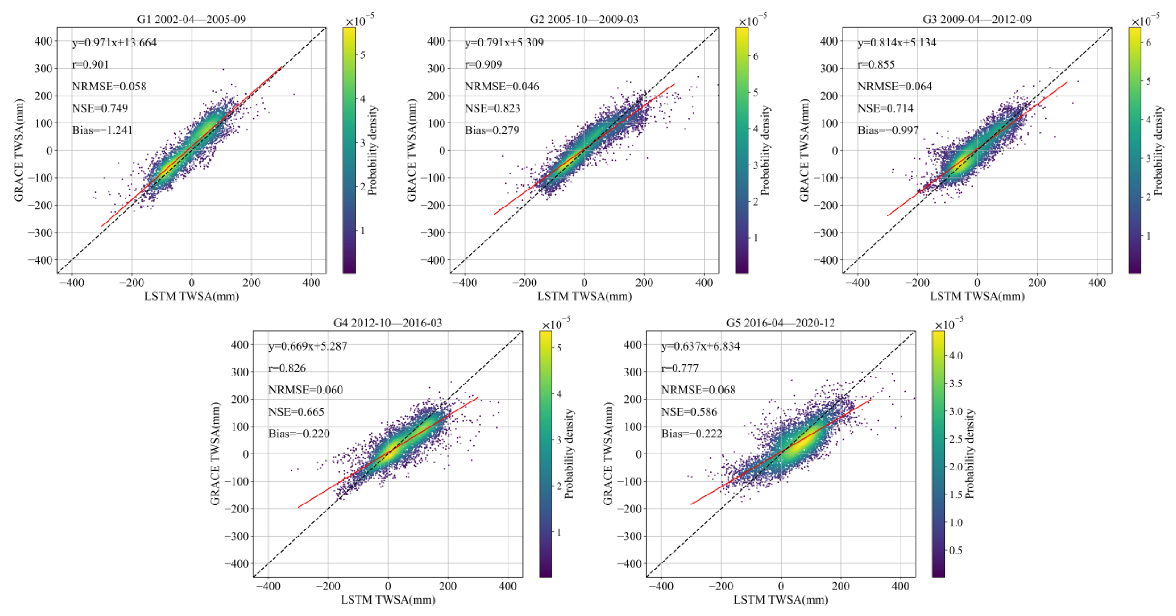
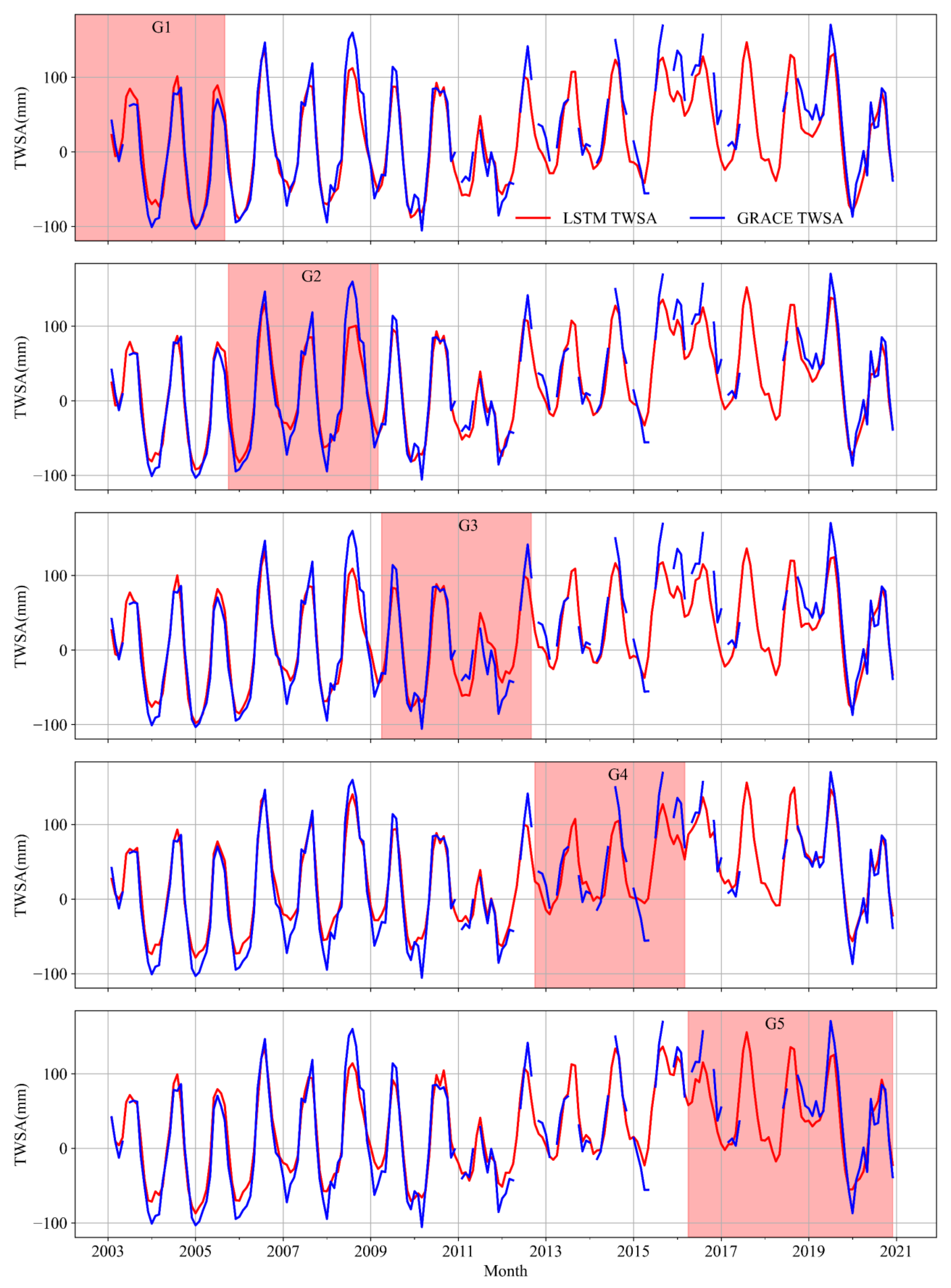
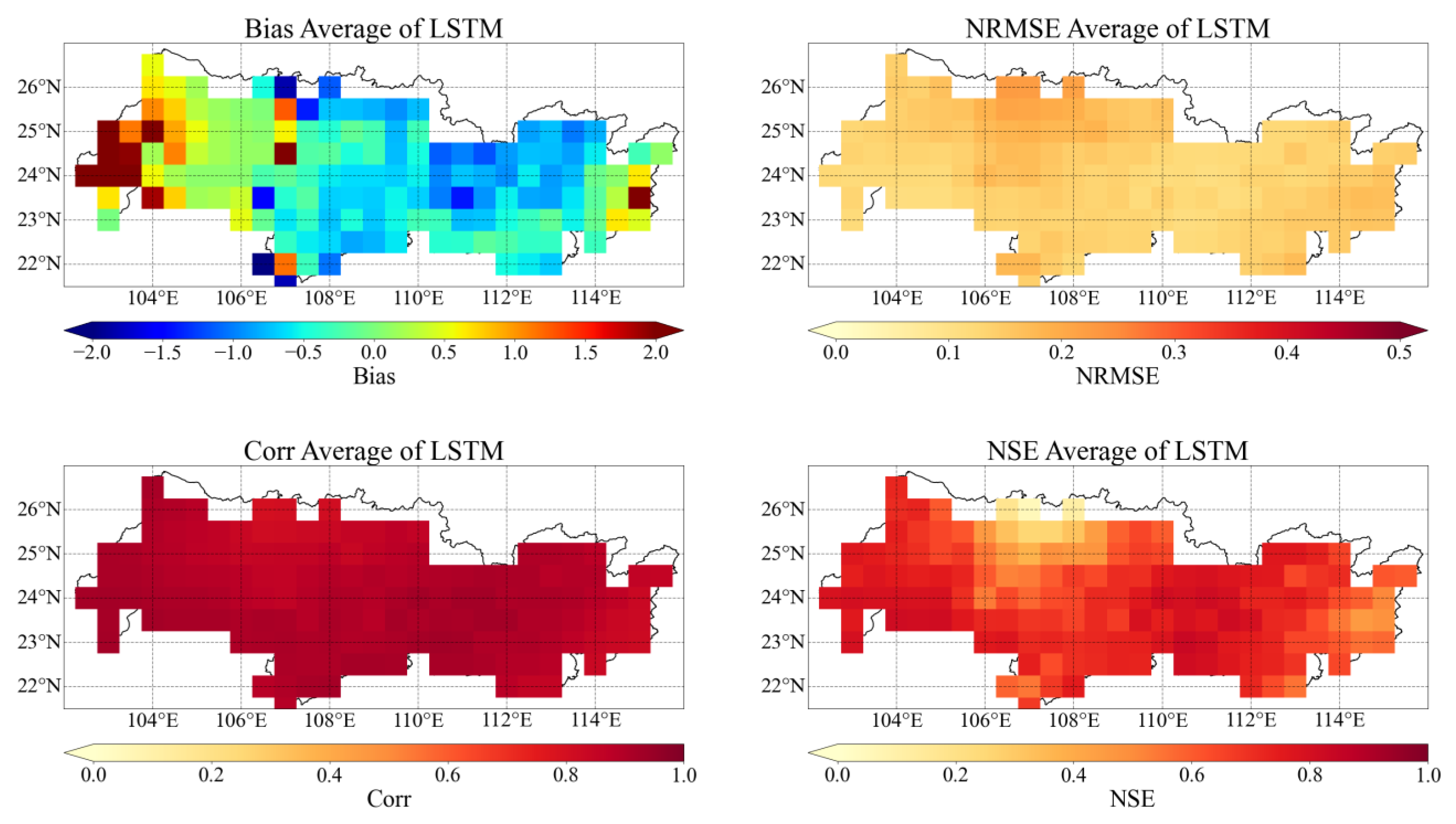
3.1. Performance of the LSTM Models

In our study, the LSTM-based models exhibited satisfactory performance overall, effectively capturing the trends in TWSA. Additionally, there was minimal difference in performance measures between the training and testing sets, indicating that the data have a relatively good representativeness and the models have been sufficiently trained. The evaluation indicators’ standard deviation (Std) across the five groups was small, suggesting a certain degree of stability in the models.
From the perspective of spatiotemporal average, the specific results are shown in Table 3. The scatter density plots (Figure 3) show that the LSTM models performed well in simulating TWSA, with correlation coefficients ranging from 0.777 to 0.909 and an average of 0.854. The NRMSE ranges from 0.046 to 0.068, with an average of 0.059. The bias ranges from −1.241 to 0.279, with an average of −0.48. The NSE is relatively high, ranging from 0.586 to 0.823, with an average of 0.707.
From the perspective of basin average, specific results are shown in Table 4. On the testing set, five groups of correlation coefficients between the simulated values and GRACE observations range from 0.957 and 0.984, with an average of 0.967. Additionally, the time series plots (Figure 4) show that the LSTM models can effectively capture the seasonal variations of TWSA. However, there is a certain gap between the simulated values and the observations at the peak values. This discrepancy can be attributed to the limited number of samples during peak periods, resulting in the model being relatively undertrained and making conservative predictions at the peaks. Overall, the LSTM model exhibits excellent performance in simulating the average TWSA of the entire basin. Therefore, analyzing the average TWSA reconstructed by LSTM can help mitigate the impact of missing months on driving factor analysis.
From a temporal average perspective, Figure 5 illustrates the spatial distribution of each evaluation metric within the basin, while specific results for five groups are provided in Table 5. In general, the correlation coefficient (r) between GRACE observations of equivalent water height and the reconstructed values for each grid point is consistently above 0.8, with more than 88% of the grid cells having a correlation coefficient greater than 0.85. Additionally, NSE exceeds 0.6 for more than 80% of the grid cells, NRMSE remains below 0.17 for over 85% of them, and bias is less than 0.9 for more than 78%. The correlation near the boundary is strong, although the degree of fitting is low. This can be attributed to the limited training of LSTM near the boundary due to the absence of data beyond it.

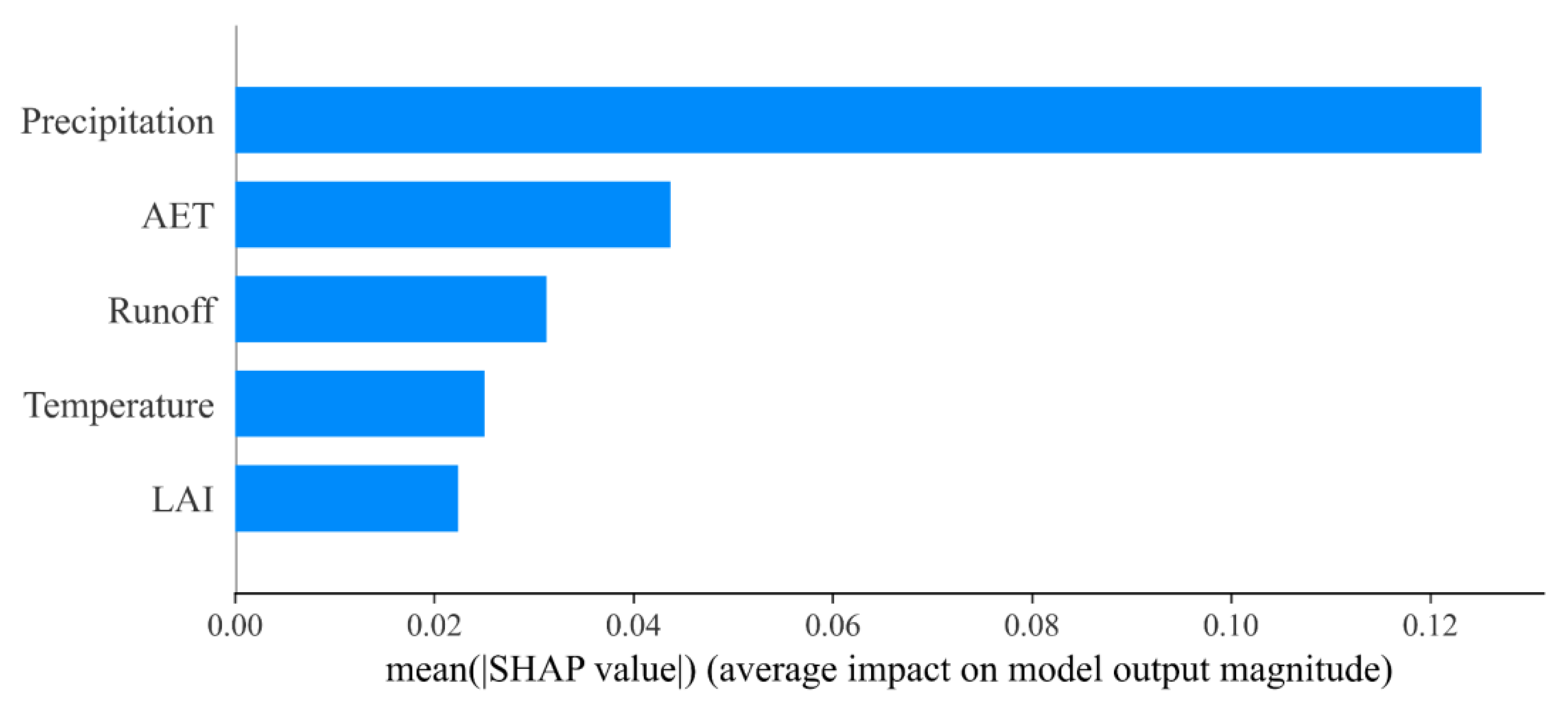
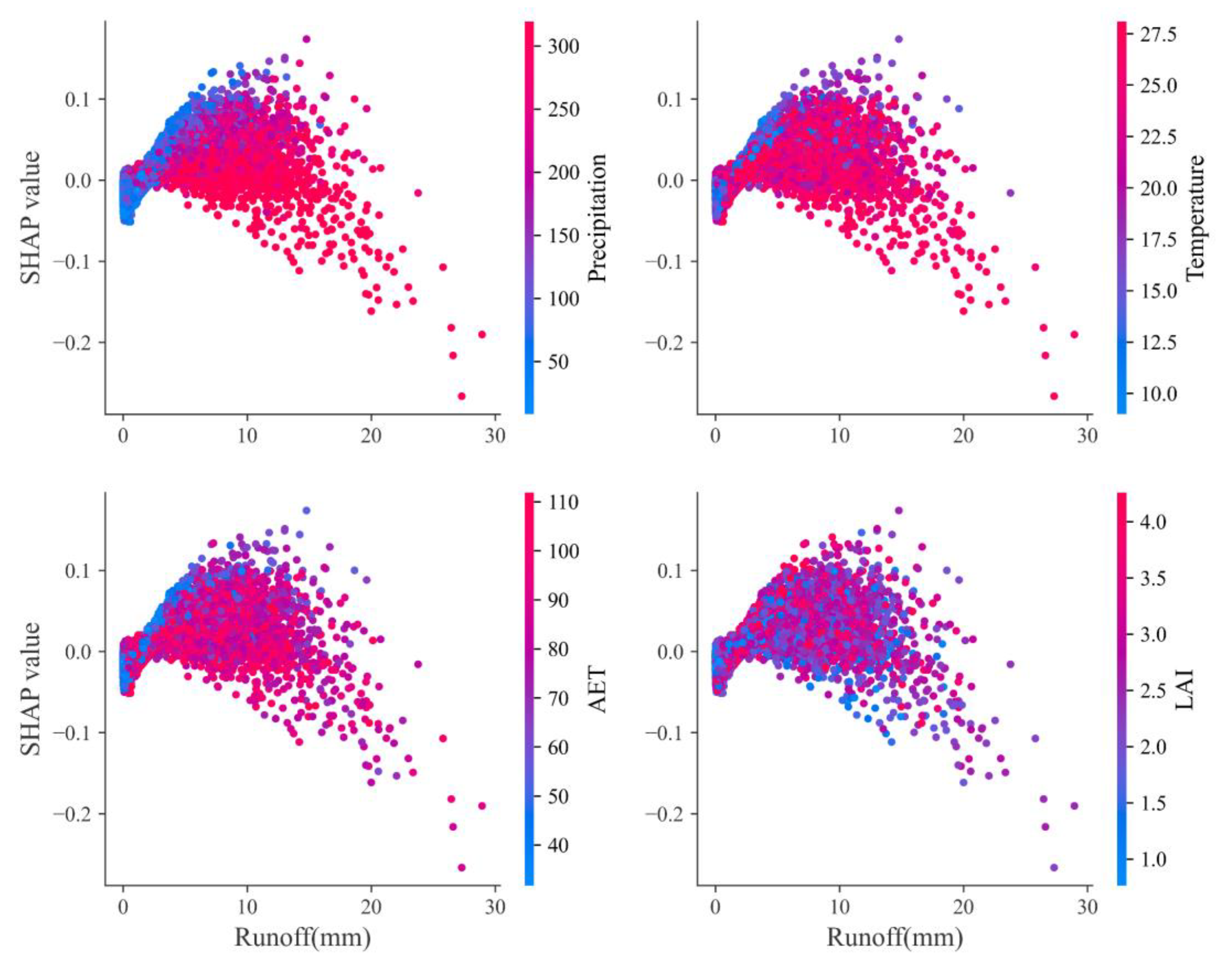
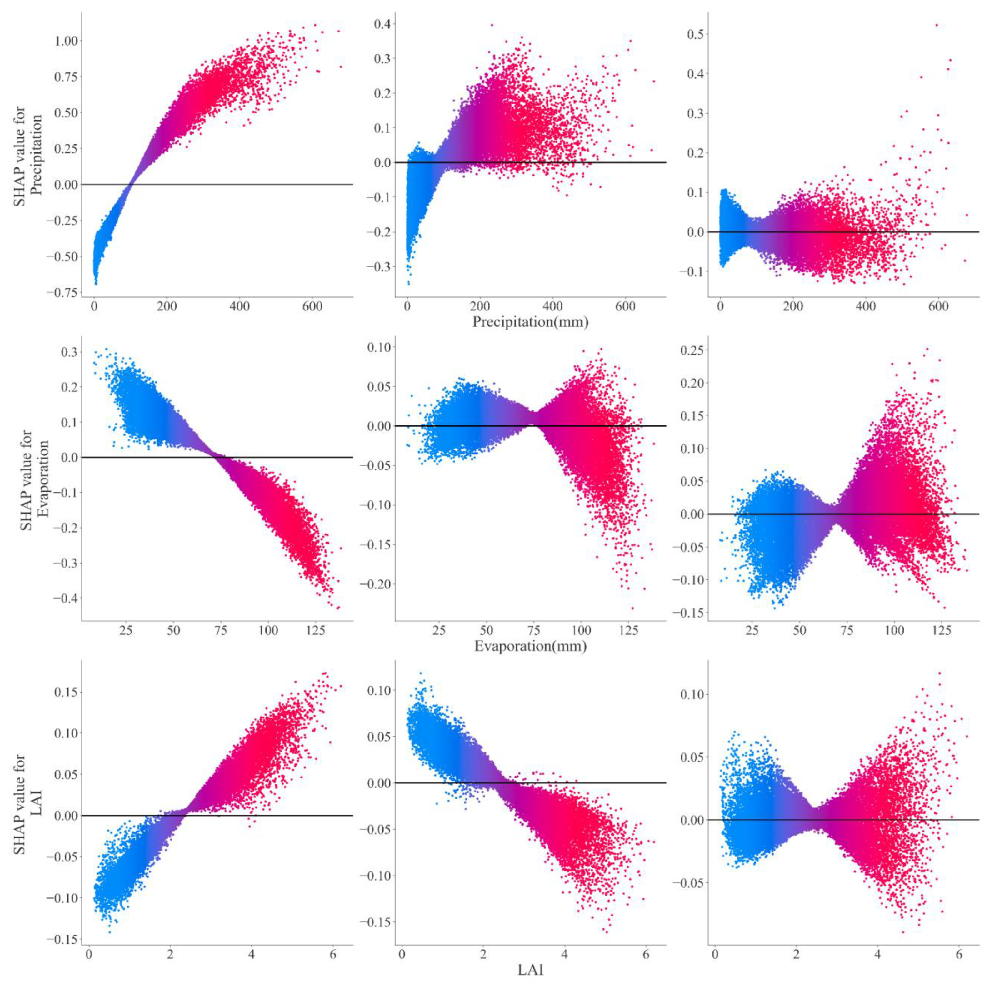
3.2. Correlation and Importance Analysis of TWSA Driving Factors Based on SHAP

TWS is influenced by precipitation, temperature, evapotranspiration, runoff, and vegetation. These driving factors interact with each other simultaneously. Thus, the linear correlation coefficient and lag correlation analysis between a single factor and TWS do not yield the desired results. For instance, according to the water balance equation, an increase in evapotranspiration and runoff can lead to a decrease in TWS, but the correlation coefficient shows that both evapotranspiration and runoff have a positive correlation with TWS (Figure 6). Therefore, accurately reflecting the correlation between driving factors and TWS requires considering the coupling effect of multiple factors. Here, we utilized a LSTM model (G2) to simulate the coupling effect compared with direct analysis between a single factor and TWSA. Additionally, we employed the SHAP method to analyze the role of each driving factor in this process.
Figure 6 shows the temporal variations of various driving factors and GRACE TWSA from a basin average perspective. Generally, all driving factors have a positive correlation with TWSA with a lead time no more than 2 months between driving factors and TWSA under the coupling effect. Furthermore, the seasonal fluctuations and correlation coefficients of each driving factor are comparable to those of TWSA (Table 6). They tend to reach their maximum and minimum values almost simultaneously with TWSA, although slight variations exist among different driving factors, indicating their different influences on TWSA.
Precipitation is the main water source for TWS and plays a key role in the hydrological water cycle, making it a crucial driving factor for TWS. In the PRB, characterized by subtropical monsoonal climate zones, precipitation exhibits distinct seasonal variations, with precipitation in summer (June–August) accounting for about 50–70% of the annual total. Hence, TWSA in the PRB displays a similar seasonal trend to precipitation. Notably, both precipitation and TWSA in the PRB show a slight upward trend between 2003 and 2020, with a substantial increase during the summer months. Furthermore, the analysis reveals a two-month time lag between peak values of TWSA and precipitation (Table 6), and the lagged correlation coefficient between precipitation and TWSA is 0.76, which is consistent with previous studies. Moreover, the lagged correlation coefficient between TWSA and runoff is smaller than that of precipitation, indicating that the response of runoff to TWSA is faster than that of precipitation, which delays the rise in the soil moisture.
The effects of evapotranspiration and temperature on TWSA are similar, as the increase in temperature leads to increased evapotranspiration, with temperature having a smaller lagged correlation coefficient. Additionally, both evapotranspiration and temperature display a lag time of one month in relation to TWSA, indicating that the replenishment of atmospheric precipitation through evapotranspiration delays the increase in TWSA.
The seasonal variations of LAI exhibit similarity to that of TWSA, with a coincident correlation coefficient of 0.79. Both LAI and TWSA show a slight upward trend, highlighting the significance of vegetation as an additional important driving factor alongside precipitation. Vegetation plays a role in intercepting precipitation, reducing runoff, and subsequently decreasing regional water exchange, which contributes to an increase in TWSA. This process occurs within a relatively short timeframe.
Figure 7 shows the importance ranking of driving factors. Generally, precipitation emerges as the most crucial driving factor, followed by evapotranspiration, runoff, temperature, and LAI. The influence of precipitation is much greater than that of any other factor, emphasizing its paramount importance.
Considering that the hydrological process represented by runoff is more complex and interacts more frequently with other driving factors, dependence plots between runoff and other driving factors are drawn to analyze the interaction between driving factors further (Figure 8). In general, runoff shows a negative correction with TWS. The impact is less pronounced when runoff amounts are small, but becomes more evident with larger runoff volumes, indicating a stronger inhibitory effect. Furthermore, the dependence plots demonstrate an obvious vertical distribution pattern, which reflects its interaction with other driving factors. Especially, larger precipitation, higher temperatures, and greater evapotranspiration contribute to both an increase in TWS and an enhanced inhibitory effect of runoff on TWS. However, LAI does not exhibit a significant impact on this interaction. These findings underscore the intricate nature of the coupling effects among driving factors.

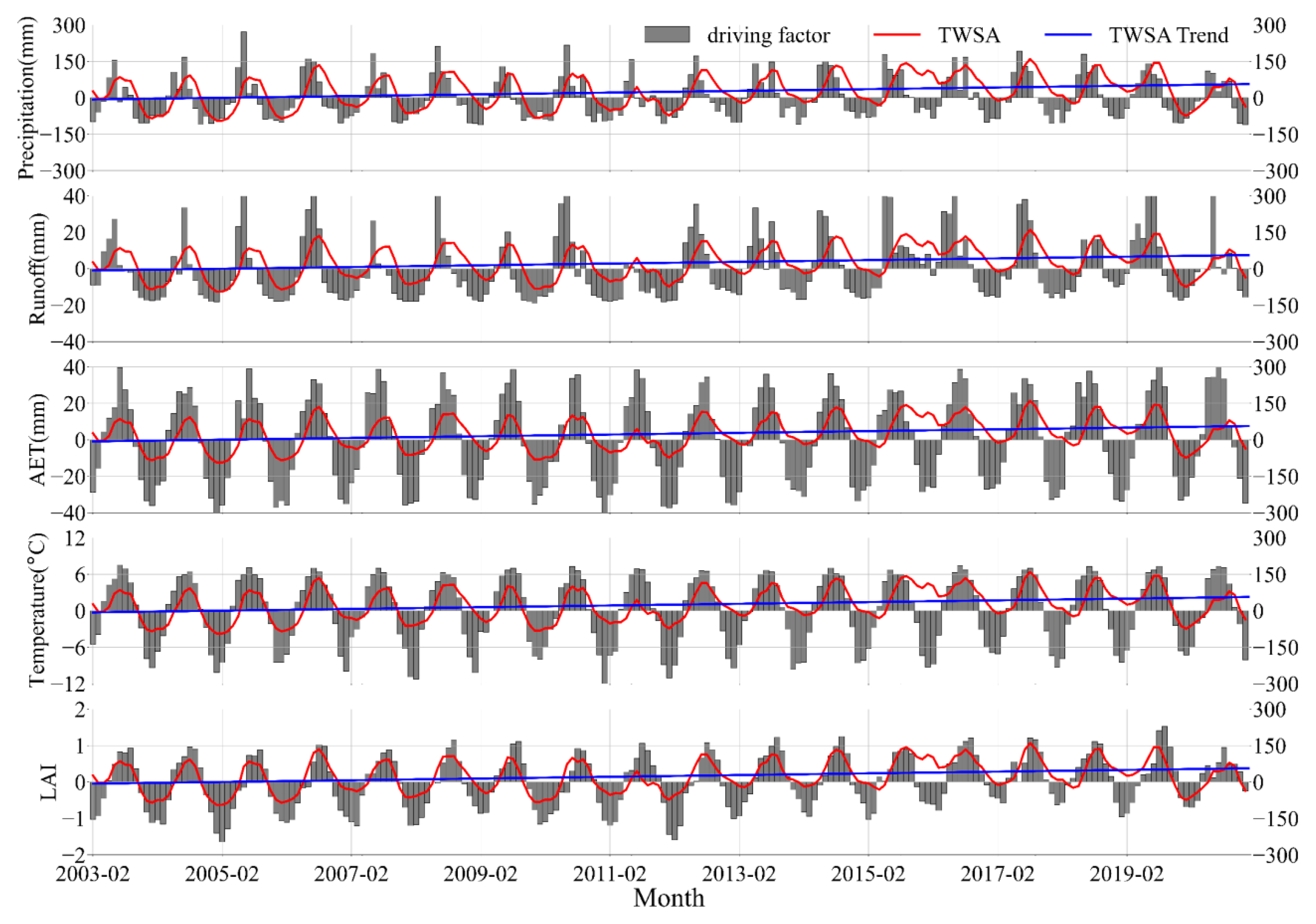
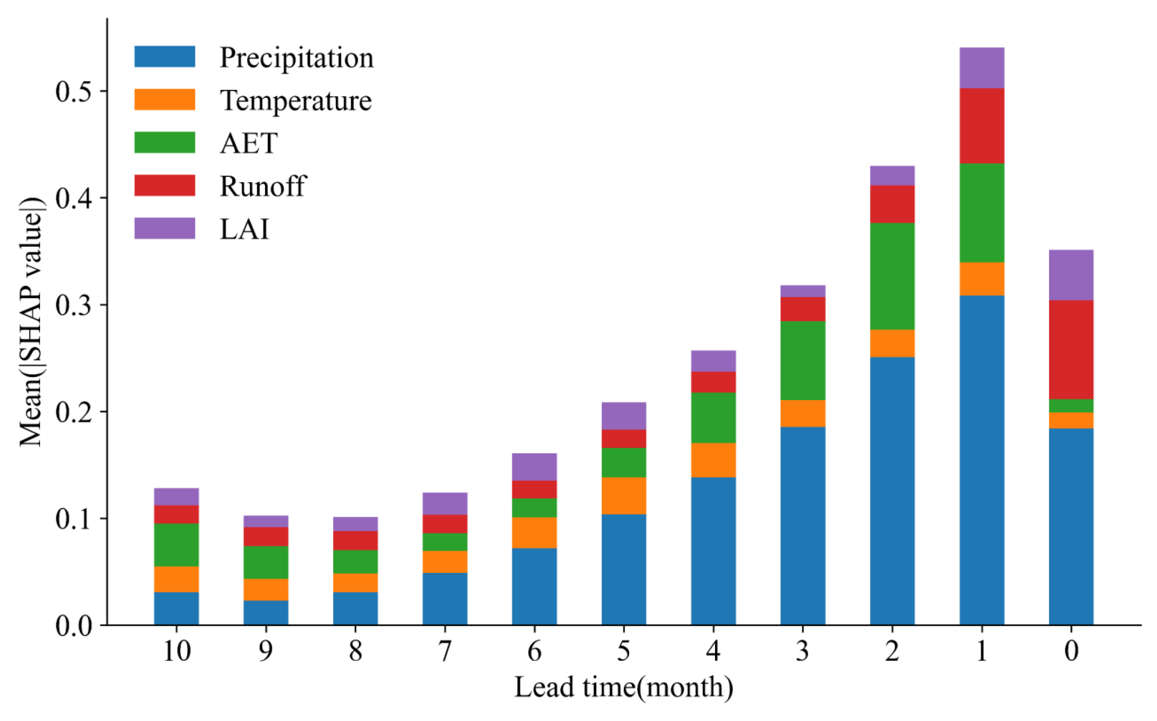
3.3. Lead Time Analysis between GRACE TWSA and Driving Factors

Figure 9 showcases the influence of different lead times for each driving factor on TWS revealed through SHAP analysis. Generally, the influence of a driving factor under the coupling effect becomes stronger as the lead time approaches the current month. The coupling effect of driving factors reaches the maximum when the lead time is one month, followed by a two-month lead time, and the current month (namely, zero lead time). Specifically, precipitation from the previous month exerts the greatest impact, while the effect of evapotranspiration is strongest with a two-month lead time. LAI and runoff have the most significant effect in the current month, whereas temperature has a relatively small and uniform impact.
Figure 10 illustrates the cumulative local effects of partial dependence plots with three different lead times on TWS in the PRB. As mentioned in the Methods section, a partial dependence plot presents the SHAP values of a driving factor at a certain lead time in each sample, representing the contribution’s change when the value of the driving factor changes. In general, the relationship between the SHAP value and its driving factors exhibits nonlinearity and nonmonotonicity on the time scale.
Figure 10 shows that the SHAP value of precipitation with longer lead times exhibits strong nonlinearity with the value of precipitation. When the precipitation is high, the SHAP value has a positive correlation with the precipitation and the SHAP value is large. However, when the precipitation is low, the SHAP value has no obvious correlation with the precipitation and the range of SHAP values is smaller. As the lead time approaches the current month, even when the precipitation is low, the SHAP value also gradually exhibits strong linearity with the value of precipitation and the range of SHAP values also becomes larger. This indicates that higher precipitation with different lead times has a significant effect on increasing the TWS in the current month, while lower precipitation has little effect. Notably, when the lead time is closer to the current month, the effect of precipitation on TWS in the current month becomes more pronounced.
In the case of evapotranspiration and temperature, they exhibit similar patterns. When the lead time is long, the range of SHAP values is small, showing no obvious correlation with the amount of evapotranspiration. As the lead time gets closer to the current month, the SHAP value gradually shows a negative correlation with evapotranspiration. This suggests that evapotranspiration with a longer lead time has less effect on TWS. As the lead time gets closer to the current month, the inhibitory effect of evaporation on the TWS in the current month is more obvious. Additionally, it is worth noting that the negative correlation cannot be drawn directly by conducting a separate correlation analysis between evapotranspiration and TWSA (Figure 6). However, the deep learning model that integrates all five driving factors can effectively identify the negative correlation of evapotranspiration on TWS.
As for LAI, it exhibits a slightly different trend compared to evapotranspiration, and its correlation with the value of LAI is significantly influenced by both the magnitude of LAI and the lead time, which is more complex. When the lead time is short, lower LAI suppresses the increase in TWS, while higher LAI promotes the increase in TWS. However, for longer lead times, this relationship is reversed.

4. Discussion

4.1. The Uncertainty of the LSTM Model

Deep learning methods have proven to be highly effective in tackling complex problems, and LSTM, in particular, excels in handling long time sequence tasks. Wang et al. [51] constructed an LSTM model to simulate GRACE TWSA in the Tarim River Basin, achieving a correlation coefficient of 0.922 and NRMSE of 0.107. In this study, the average of correlation coefficient and NSE of TWSA, evaluated through 5-fold cross-validation in the PRB, are 0.854 and 0.707, respectively, from a spatiotemporal perspective. Moreover, when examining the basin average from a temporal perspective, the correlation coefficient and NSE reach high values of 0.967 and 0.912, respectively. These results highlight the outstanding capability of LSTM models in simulating time series data.
While LSTM can effectively simulate TWSA, it still introduces a certain level of uncertainty. This uncertainty primarily stems from inherent model structure limitations and potential shortcomings in training. Regarding the model structure, researchers need to carefully adjust it based on specific application scenarios. Although LSTM has good performance in temporal simulation, it may struggle to capture spatial patterns adequately, as evidenced by average correlation coefficients of 0.927 and 0.967 for spatial and temporal dimensions, respectively. However, TWS is often influenced by factors in neighboring areas, which makes spatial considerations important.
Shortcomings in training can be attributed to both the training data and model optimization. First, the limited time scale of data available (only 20 years since the launch of the GRACE satellites) poses challenges in effectively training the model. Treating each time grid point in the basin as a separate sample increased the sample size but introduced the uncertainty in the spatial distribution of TWSA patterns. Moreover, factors such as human activities and geographical conditions, which are not considered in the model, can also impact TWS. Additionally, the data themselves also carry inherent uncertainty.
As for optimization, as can be seen from Table 3, Table 4 and Table 5, the LSTM model always performs better on the training set than on the testing set. Ideally, both the training and testing sets should obey the same data distribution. The LSTM model learns the joint probability distribution of the training set and applies it to the testing set. However, due to the inability to consider all factors, variations in other factors may lead to the invalidity of this assumption, especially when the training and testing data come from different time periods. Consequently, the performance of the model on the testing set may not be as strong as on the training set [47]. As can be seen from the scatter plots (Figure 3), the model tends to be conservative in its simulation of peak values. This may be due to the uneven distribution of the samples and inherent model characteristics. The proportion of peak values in periodic data is small, making it challenging to train the model effectively. Additionally, the spatial distribution figure (Figure 5) indicates a scarcity of data around the edges of the basin, which partially reduces the effectiveness of the simulation.

4.2. Analysis of Natural Driving Factors

Figure 9 illustrates that these driving factors exert distinct hysteresis effects on TWS, a phenomenon corroborated by previous studies. Wang et al. [52] found the hysteresis effect from precipitation, explaining that the TWS for a given month only incorporates precipitation information from the preceding month. This is due to the time required for precipitation infiltration and evaporation processes. We thus delve into the hysteresis of different driving factors in the GRACE-derived monthly TWS to examine their temporal impacts on TWS.
From Figure 9, it is evident that runoff exhibits its greatest impact in the current month. Meanwhile, precipitation from the previous month and evapotranspiration from two months prior exert stronger influences. We postulate that this is due to GRACE’s measurement techniques and the hydrological cycle. GRACE likely exhibits heightened sensitivity to substantial water body quality fluctuations, encompassing rivers, lakes, and groundwater. This leads to spatial and temporal hysteresis variations. Figure 9 highlights the most immediate TWS responses to the runoff since runoff aptly represents rivers and lakes. Some of the runoff seeps into the soil, needing time to reach groundwater, thereby influencing the subsequent month’s TWS.
The situation of the precipitation is different from runoff. Upon reaching the land surface, precipitation transforms into major hydrological components, including runoff, soil moisture, groundwater, and evapotranspiration. We observe that precipitation has the highest impact on TWS at a one-month lead time (Figure 9). This indicates that the combined amount of runoff, soil moisture, groundwater, and evapotranspiration is predominantly determined by the precipitation from the preceding month. In other words, the TWS response to precipitation is most significant with a one-month lag, highlighting the time required for these hydrological processes to take effect.
Temperature affects plant growth and evapotranspiration. Its contribution pattern over the initial three months mirrors that of evaporation. However, since temperature can also influence precipitation and plant growth, it adds complexity to the relationship between TWS and temperature.
Compared to temperature and precipitation, the hysteresis effect of evapotranspiration is more pronounced. Apart from its impact on lakes or rivers, evapotranspiration mainly influences TWS by depleting soil moisture and groundwater. These processes take longer to manifest, explaining why evapotranspiration from the previous two months has a more significant impact on TWS. Moreover, evapotranspiration is also affected by temperature and soil moisture, indicating a potential reciprocal influence on TWS.
Lastly, vegetation’s influence on TWS is multifaceted. It can modify soil moisture, significantly impact both runoff and evapotranspiration, and consume varied water amounts at different stages of plant growth. Figure 9 suggests that in the PRB, vegetation shows a similar trend to runoff, indicating that vegetation primarily influences TWS by altering runoff patterns.

4.3. Uncertainty of Explainable Machine Learning

Machine learning models have been widely used in Earth science for their excellent performance in stimulating complex nonlinear processes, even without prior assumptions about the underlying physical systems. However, one challenge associated with machine learning models, particularly deep learning models, is their lack of interpretability. To address this issue, explainable machine learning was introduced by the Defense Advanced Research Projects Agency in 2017, and it has gained popularity across various fields, especially in scientific research [53]. Several machine learning interpretation techniques, such as LIME and ALE, have been developed and applied to elucidate the patterns captured by these models. Previous studies have demonstrated the significant capabilities of explainable machine learning in revealing complex natural processes. In this study, we utilized the SHAP method to quantify the relative contributions of precipitation, temperature, vegetation, runoff, and evapotranspiration to TWS. Notably, the results align with the existing understanding of hydrological processes from previous studies, indicating a certain level of explanatory power for hydrological phenomena.
However, the SHAP method used in this study introduces its own uncertainty. Firstly, SHAP is a method of additive interpretation that assigns an additive contribution value to each variable. However, this method can be affected by multicollinearity between variables, which reduces the reliability of the model when there is high interaction among driving factors. Additionally, the learning ability of the deep learning model is a crucial factor in the interpretability of the results obtained through explainable techniques. It is essential for the deep learning model to capture the physical laws of the research objects rather than solely relying on correlations for prediction. The deep learning model structure itself also introduces uncertainty in the attribution allocation. While LSTM can mitigate the issue of gradient vanishing, it cannot completely balance the difficulty of gradient updating at different time steps. Some scholars believe that due to the existence of forget gates in LSTM, the model tends to consider the influence of similar factors over time [24].
Despite the inherent uncertainties and limitations associated with data-driven methods such as deep learning and interpretable machine learning methods, they offer researchers valuable modeling techniques to accurately estimate TWS and comprehend water cycles [54]. Such methods have the potential to unveil complex relationships that have not yet been observed or are challenging to observe through traditional approaches.
For future work, we aim to incorporate additional driving factors into our models, including human activities, soil texture, and other relevant variables. Furthermore, we aim to explore models that incorporate both temporal and spatial aspects, such as convolutional neural networks and spatiotemporal convolutional neural networks. By comparing and utilizing datasets with less uncertainty, we can enhance the robustness of our simulations. Additionally, we will incorporate spatial interpretation methods, such as gradient-weighted class activation mapping (Grad-CAM), to improve the interpretability of our models and make the simulation and interpretation more reasonable.

5. Conclusions

In this study, a long short-term memory (LSTM) neural network model, based on the data of precipitation, runoff, evapotranspiration, temperature, and leaf area index (LAI), was applied to simulate terrestrial water storage anomaly (TWSA) combined with GRACE gravity satellite products. We employed the SHapley Additive exPlanations (SHAP) method to quantitatively analyze the contributions of different driving factors to terrestrial water storage (TWS) in the Pearl River Basin (PRB) and explored the impacts of different lead times. Our results show that the LSTM model performs well in stimulating TWSA. From the perspective of the basin average, the basin-average r is 0.967 and NSE is 0.912. Moreover, our modeled findings demonstrated that TWSA in the PRB is predominately influenced by precipitation, followed by evapotranspiration, runoff, temperature, and LAI. There is also a clear accumulation effect of precipitation and evapotranspiration on TWS, which becomes more obvious with a shorter lead time in general. Finally, the impact of driving factors on TWS is related to lead time. Precipitation exerts the most significant effect with a lead time of one month, while that of evapotranspiration reaches its peak impact when the lead time is one to two months. Runoff has the greatest effect in the current month, while the effect of the lead time of temperature on TWS is relatively minor.

Author Contributions

Conceptualization, H.H., G.F. (Guanbin Feng) and X.C.; methodology, H.H., G.F. (Guanbin Feng) and G.F. (Guanning Feng); software, H.H., G.F. (Guanbin Feng), Y.C. and G.F. (Guanning Feng); validation, H.H.; formal analysis, Y.C.; investigation, G.F. (Guanbin Feng), G.F. (Guanning Feng), Z.D., J.W. and P.T.; data curation, Y.C.; writing—original draft preparation, H.H., G.F. (Guanbin Feng), Z.D. and P.T.; writing—review and editing, X.C.; supervision, X.C.; project administration, H.H.; funding acquisition, X.C. All authors have read and agreed to the published version of the manuscript.

Funding

This work was supported by the Innovation and Entrepreneurship Training Program for College Students of Sun Yat-sen University and the Natural Science Foundation of Guangdong Province, China (2022A1515010676).

Data Availability Statement

Monthly TWS data were obtained from the NASA Goddard Space Flight Center (GSFC) at https://earth.gsfc.nasa.gov/geo/data/grace-mascons (accessed on 11 October 2022). Climate Research Unit (CRU) monthly precipitation data were downloaded from https://crudata.uea.ac.uk/cru/data/hrg/ (accessed on 3 November 2022). The monthly actual evapotranspiration (AET) data were extracted from the Global Land Evaporation Amsterdam Model (GLEAM) from https://www.gleam.eu/ (accessed on 3 November 2022). The runoff data released by the European Centre for Medium-range Weather Forecasts ReAnalysis 5-Land (ERA5-Land) reanalysis dataset were downloaded at https://cds.climate.copernicus.eu/cdsapp#!/dataset/reanalysis-era5-land-monthly-means (accessed on 14 November 2022). The monthly leaf area index (LAI) was downloaded from the Land-Atmosphere Interaction Research Group at Sun Yat-sen University (SYSU) at http://globalchange.bnu.edu.cn/research/laiv061 (accessed on 19 November 2022).

Acknowledgments

The authors would like to acknowledge the valuable comments on the manuscript provided by the editors and anonymous reviewers.

Conflicts of Interest

The authors declare no conflict of interest.

References

  1. Li, F.P.; Kusche, J.; Chao, N.F.; Wang, Z.T.; Locher, A. Long-Term (1979–Present) Total Water Storage Anomalies Over the Global Land Derived by Reconstructing GRACE Data. Geophys. Res. Lett. 2021, 48, e2021GL093492. [Google Scholar] [CrossRef]
  2. Rodell, M.; Famiglietti, J.S.; Wiese, D.N.; Reager, J.T.; Beaudoing, H.K.; Landerer, F.W.; Lo, M.H. Emerging trends in global freshwater availability. Nature 2019, 565, E7. [Google Scholar] [CrossRef]
  3. Xie, X.M.; He, B.; Guo, L.L.; Miao, C.Y.; Zhang, Y.F. Detecting hotspots of interactions between vegetation greenness and terrestrial water storage using satellite observations. Remote Sens. Environ. 2019, 231, 111259. [Google Scholar] [CrossRef]
  4. Kusche, J.; Eicker, A.; Forootan, E.; Springer, A.; Longuevergne, L. Mapping probabilities of extreme continental water storage changes from space gravimetry. Geophys. Res. Lett. 2016, 43, 8026–8034. [Google Scholar] [CrossRef] [Green Version]
  5. Huang, Z.Y.; Jiao, J.J.; Luo, X.; Pan, Y.; Jin, T.Y. Drought and Flood Characterization and Connection to Climate Variability in the Pearl River Basin in Southern China Using Long-Term GRACE and Reanalysis Data. J. Clim. 2021, 34, 2053–2078. [Google Scholar] [CrossRef]
  6. Pokhrel, Y.; Felfelani, F.; Satoh, Y.; Boulange, J.; Burek, P.; Gadeke, A.; Gerten, D.; Gosling, S.N.; Grillakis, M.; Gudmundsson, L.; et al. Global terrestrial water storage and drought severity under climate change. Nat. Clim. Change 2021, 11, 226–233. [Google Scholar] [CrossRef]
  7. Luo, Z.; Yao, C.; Li, Q.; Huang, Z.J. Terrestrial water storage changes over the Pearl River Basin from GRACE and connections with Pacific climate variability. Geod. Geodyn. 2016, 7, 171–179. [Google Scholar] [CrossRef] [Green Version]
  8. Wahr, J.; Swenson, S.; Zlotnicki, V.; Velicogna, I. Time-variable gravity from GRACE: First results. Geophys. Res. Lett. 2004, 31, 11. [Google Scholar] [CrossRef] [Green Version]
  9. Deng, H.J.; Chen, Y.N.; Chen, X.W. Driving factors and changes in components of terrestrial water storage in the endorheic Tibetan Plateau. J. Hydrol. 2022, 612, 128225. [Google Scholar] [CrossRef]
  10. Guo, F.; Jiang, G.H.; Yuan, D.X.; Polk, J.S. Evolution of major environmental geological problems in karst areas of Southwestern China. Environ. Earth Sci. 2013, 69, 2427–2435. [Google Scholar] [CrossRef]
  11. Yao, C.L.; Luo, Z.C. Karstic water storage response to the recent droughts in Southwest China estimated from satellite gravimetry. Int. Conf. Intell. Earth Obs. Appl. 2015, 9808, 334–339. [Google Scholar]
  12. Sun, A.Y.; Scanlon, B.R. How can Big Data and machine learning benefit environment and water management: A survey of methods, applications, and future directions. Environ. Res. Lett. 2019, 14, 073001. [Google Scholar] [CrossRef]
  13. Hamshaw, S.D.; Dewoolkar, M.M.; Schroth, A.W.; Wemple, B.C.; Rizzo, D.M. A New Machine-Learning Approach for Classifying Hysteresis in Suspended-Sediment Discharge Relationships Using High-Frequency Monitoring Data. Water Resour. Res. 2018, 54, 4040–4058. [Google Scholar] [CrossRef]
  14. Reichstein, M.; Camps-Valls, G.; Stevens, B.; Jung, M.; Denzler, J.; Carvalhais, N.; Prabhat. Deep learning and process understanding for data-driven Earth system science. Nature 2019, 566, 195–204. [Google Scholar] [CrossRef]
  15. Xue, M.; Hang, R.L.; Liu, Q.S.; Yuan, X.T.; Lu, X.Y. CNN-based near-real-time precipitation estimation from Fengyun-2 satellite over Xinjiang, China. Atmos. Res. 2021, 250, 105337. [Google Scholar] [CrossRef]
  16. Huang, X.; Gao, L.; Crosbie, R.S.; Zhang, N.; Fu, G.B.; Doble, R. Groundwater Recharge Prediction Using Linear Regression, Multi-Layer Perception Network, and Deep Learning. Water 2019, 11, 1879. [Google Scholar] [CrossRef] [Green Version]
  17. Kratzert, F.; Klotz, D.; Brenner, C.; Schulz, K.; Herrnegger, M. Rainfall-runoff modelling using Long Short-Term Memory (LSTM) networks. Hydrol. Earth Syst. Sci. 2018, 22, 6005–6022. [Google Scholar] [CrossRef] [Green Version]
  18. Long, D.; Shen, Y.J.; Sun, A.; Hong, Y.; Longuevergne, L.; Yang, Y.T.; Li, B.; Chen, L. Drought and flood monitoring for a large karst plateau in Southwest China using extended GRACE data. Remote Sens. Environ. 2014, 155, 145–160. [Google Scholar] [CrossRef]
  19. Qiu, R.J.; Wang, Y.K.; Rhoads, B.; Wang, D.; Qiu, W.J.; Tao, Y.W.; Wu, J.C. River water temperature forecasting using a deep learning method. J. Hydrol. 2021, 595, 126016. [Google Scholar] [CrossRef]
  20. Mo, S.X.; Zhong, Y.L.; Forootan, E.; Mehrnegar, N.; Yin, X.; Wu, J.C.; Feng, W.; Shi, X.Q. Bayesian convolutional neural networks for predicting the terrestrial water storage anomalies during GRACE and GRACE-FO gap. J. Hydrol. 2022, 604, 127244. [Google Scholar] [CrossRef]
  21. Fang, K.; Pan, M.; Shen, C.P. The Value of SMAP for Long-Term Soil Moisture Estimation With the Help of Deep Learning. IEEE Trans. Geosci. Remote Sens. 2019, 57, 2221–2233. [Google Scholar] [CrossRef]
  22. Cheng, S.J.; Cheng, L.; Qin, S.J.; Zhang, L.; Liu, P.; Liu, L.; Xu, Z.C.; Wang, Q.L. Improved Understanding of How Catchment Properties Control Hydrological Partitioning Through Machine Learning. Water Resour. Res. 2022, 58, e2021WR031412. [Google Scholar] [CrossRef]
  23. Li, L.Y.; Zeng, Z.Z.; Zhang, G.; Duan, K.; Liu, B.J.; Cai, X.T. Exploring the Individualized Effect of Climatic Drivers on MODIS Net Primary Productivity through an Explainable Machine Learning Framework. Remote Sens. 2022, 14, 4401. [Google Scholar] [CrossRef]
  24. Jiang, S.J.; Zheng, Y.; Wang, C.; Babovic, V. Uncovering Flooding Mechanisms Across the Contiguous United States Through Interpretive Deep Learning on Representative Catchments. Water Resour. Res. 2022, 58, e2021WR030185. [Google Scholar] [CrossRef]
  25. Kondylatos, S.; Prapas, I.; Ronco, M.; Papoutsis, I.; Camps-Valls, G.; Piles, M.; Fernandez-Torres, M.A.; Carvalhais, N. Wildfire Danger Prediction and Understanding With Deep Learning. Geophys. Res. Lett. 2022, 49, e2022GL099368. [Google Scholar] [CrossRef]
  26. Sihi, D.; Dari, B.; Kuruvila, A.P.; Jha, G.; Basu, K. Explainable Machine Learning Approach Quantified the Long-Term (1981–2015) Impact of Climate and Soil Properties on Yields of Major Agricultural Crops Across CONUS. Front. Sustain. Food Syst. 2022, 6, 847892. [Google Scholar] [CrossRef]
  27. Sonnewald, M.; Lguensat, R. Revealing the Impact of Global Heating on North Atlantic Circulation Using Transparent Machine Learning. J. Adv. Model. Earth Syst. 2021, 13, e2021MS002496. [Google Scholar] [CrossRef]
  28. Fan, M.; Zhang, L.J.; Liu, S.Y.; Yang, T.T.; Lu, D. Investigation of hydrometeorological influences on reservoir releases using explainable machine learning methods. Front. Water 2023, 5, 1112970. [Google Scholar] [CrossRef]
  29. Cai, X.; Li, L.; Fisher, J.B.; Zeng, Z.; Zhou, S.; Tan, X.; Liu, B.; Chen, X. The responses of ecosystem water use efficiency to CO2, nitrogen deposition, and climatic drivers across China. J. Hydrol. 2023, 622, 129696. [Google Scholar] [CrossRef]
  30. Lundberg, S.M.; Lee, S.I. A Unified Approach to Interpreting Model Predictions. Adv. Neural Inf. Process. Syst. 2017, 30. [Google Scholar]
  31. Lundberg, S.M.; Erion, G.G.; Lee, S.-I. Consistent individualized feature attribution for tree ensembles. arXiv 2018, arXiv:1802.03888. [Google Scholar]
  32. Sun, Z.L.; Long, D.; Yang, W.T.; Li, X.Y.; Pan, Y. Reconstruction of GRACE Data on Changes in Total Water Storage Over the Global Land Surface and 60 Basins. Water Resour. Res. 2020, 56, e2019WR026250. [Google Scholar] [CrossRef]
  33. Pearl River Water Resources Committee (PRWRC). The Zhujiang Archive; Guangdong Science and Technology Press: Guangzhou, China, 1991; Volume 1. (In Chinese) [Google Scholar]
  34. Lü-Liu, L.; Tong, J.; Jin-Ge, X.; Jian-Qing, Z.; Yong, L.J. Responses of hydrological processes to climate change in the Zhujiang River basin in the 21st century. Adv. Clim. Change Res. 2012, 3, 84–91. [Google Scholar] [CrossRef]
  35. Zhang, Q.; Xiao, M.Z.; Singh, V.P.; Li, J.F. Regionalization and spatial changing properties of droughts across the Pearl River basin, China. J. Hydrol. 2012, 472, 355–366. [Google Scholar] [CrossRef]
  36. Zhang, Q.; Singh, V.P.; Peng, J.T.; Chen, Y.D.; Li, J.F. Spatial-temporal changes of precipitation structure across the Pearl River basin, China. J. Hydrol. 2012, 440, 113–122. [Google Scholar] [CrossRef]
  37. Loomis, B.D.; Luthcke, S.B.; Sabaka, T.J. Regularization and error characterization of GRACE mascons. J. Geod. 2019, 93, 1381–1398. [Google Scholar] [CrossRef]
  38. Scanlon, B.R.; Zhang, Z.Z.; Save, H.; Wiese, D.N.; Landerer, F.W.; Long, D.; Longuevergne, L.; Chen, J.L. Global evaluation of new GRACE mascon products for hydrologic applications. Water Resour. Res. 2016, 52, 9412–9429. [Google Scholar] [CrossRef] [Green Version]
  39. Murdoch, W.J.; Singh, C.; Kumbier, K.; Abbasi-Asl, R.; Yu, B. Definitions, methods, and applications in interpretable machine learning. Proc. Natl. Acad. Sci. USA 2019, 116, 22071–22080. [Google Scholar] [CrossRef] [PubMed] [Green Version]
  40. Harris, I.; Osborn, T.J.; Jones, P.; Lister, D. Version 4 of the CRU TS monthly high-resolution gridded multivariate climate dataset. Sci. Data 2020, 7, 109. [Google Scholar] [CrossRef] [PubMed] [Green Version]
  41. Martens, B.; Miralles, D.G.; Lievens, H.; van der Schalie, R.; de Jeu, R.A.M.; Fernandez-Prieto, D.; Beck, H.E.; Dorigo, W.A.; Verhoest, N.E.C. GLEAM v3: Satellite-based land evaporation and root-zone soil moisture. Geosci. Model Dev. 2017, 10, 1903–1925. [Google Scholar] [CrossRef] [Green Version]
  42. Miralles, D.G.; Holmes, T.R.H.; De Jeu, R.A.M.; Gash, J.H.; Meesters, A.G.C.A.; Dolman, A.J. Global land-surface evaporation estimated from satellite-based observations. Hydrol. Earth Syst. Sci. 2011, 15, 453–469. [Google Scholar] [CrossRef] [Green Version]
  43. Lin, W.Y.; Yuan, H.; Dong, W.Z.; Zhang, S.P.; Liu, S.F.; Wei, N.; Lu, X.J.; Wei, Z.W.; Hu, Y.; Dai, Y.J. Reprocessed MODIS Version 6.1 Leaf Area Index Dataset and Its Evaluation for Land Surface and Climate Modeling. Remote Sens. 2023, 15, 1780. [Google Scholar] [CrossRef]
  44. Yuan, H.; Dai, Y.J.; Xiao, Z.Q.; Ji, D.Y.; Shangguan, W. Reprocessing the MODIS Leaf Area Index products for land surface and climate modelling. Remote Sens. Environ. 2011, 115, 1171–1187. [Google Scholar] [CrossRef]
  45. Hochreiter, S.; Schmidhuber, J. Long short-term memory. Neural Comput. 1997, 9, 1735–1780. [Google Scholar] [CrossRef] [PubMed]
  46. Jing, W.L.; Zhao, X.D.; Yao, L.; Di, L.P.; Yang, J.; Li, Y.; Guo, L.Y.; Zhou, C.H. Can Terrestrial Water Storage Dynamics be Estimated From Climate Anomalies? Earth Space Sci. 2020, 7, e2019EA000959. [Google Scholar] [CrossRef] [Green Version]
  47. Chen, X.; Wang, S.; Gao, H.; Huang, J.; Shen, C.; Li, Q.; Qi, H.; Zheng, L.; Liu, M. Comparison of deep learning models and a typical process-based model in glacio-hydrology simulation. J. Hydrol. 2022, 615, 128562. [Google Scholar] [CrossRef]
  48. Kingma, D.P.; Ba, J. Adam: A method for stochastic optimization. arXiv 2014, arXiv:1412.6980. [Google Scholar]
  49. Srivastava, N.; Hinton, G.; Krizhevsky, A.; Sutskever, I.; Salakhutdinov, R. Dropout: A Simple Way to Prevent Neural Networks from Overfitting. J. Mach. Learn. Res. 2014, 15, 1929–1958. [Google Scholar]
  50. Strumbelj, E.; Kononenko, I. Explaining prediction models and individual predictions with feature contributions. Knowl. Inf. Syst. 2014, 41, 647–665. [Google Scholar] [CrossRef]
  51. Wang, F.; Chen, Y.N.; Li, Z.; Fang, G.H.; Li, Y.P.; Wang, X.X.; Zhang, X.Q.; Kayumba, P.M. Developing a Long Short-Term Memory (LSTM)-Based Model for Reconstructing Terrestrial Water Storage Variations from 1982 to 2016 in the Tarim River Basin, Northwest China. Remote Sens. 2021, 13, 889. [Google Scholar] [CrossRef]
  52. Wang, J.; Huang, Y.; Cao, Y.; Wang, Y. Spatial and temporal variation of water storage in recent seven years from GRACE in Yunnan Province. Water Sav. Irrig. 2012, 5, 1–5. [Google Scholar]
  53. Adadi, A.; Berrada, M. Peeking Inside the Black-Box: A Survey on Explainable Artificial Intelligence (XAI). IEEE Access 2018, 6, 52138–52160. [Google Scholar] [CrossRef]
  54. Sun, A.Y.; Scanlon, B.R.; Zhang, Z.; Walling, D.; Bhanja, S.N.; Mukherjee, A.; Zhong, Z. Combining Physically Based Modeling and Deep Learning for Fusing GRACE Satellite Data: Can We Learn From Mismatch? Water Resour. Res. 2019, 55, 1179–1195. [Google Scholar] [CrossRef] [Green Version]
Figure 1. Geographical location and elevation distribution of the PRB. Drawing review number is GS(2020)4619.
Remotesensing 15 03983 g001
Figure 2. (a) Internal structure of LSTM memory cell; (b) the architecture of the LSTM model and its layer components with their types and the dimensions of data; (c) chain structure of the LSTM model.
Remotesensing 15 03983 g002
Figure 3. Scatter density plots between the simulated values and GRACE observations of five groups.
Remotesensing 15 03983 g003
Figure 4. Time series plots between LSTM-based and GRACE-based basin-averaged TWSA in five groups (all missing values of GRACE TWSA are dropped).
Remotesensing 15 03983 g004
Figure 5. Spatial distributions of each evaluation metric.
Remotesensing 15 03983 g005
Figure 6. Temporal variations between GRACE TWSA and each driving factor from the perspective of basin average (all driving factors are subtracted from the average value from 2003 to 2020).
Remotesensing 15 03983 g006
Figure 7. Importance ranking of driving factors of TWSA.
Remotesensing 15 03983 g007
Figure 8. Dependence plots between runoff and other driving factors.
Remotesensing 15 03983 g008
Figure 9. Importance-based ranking of driving factors for different lead times.
Remotesensing 15 03983 g009
Figure 10. Partial dependence plots with different lead times (the lead times of the three driving factors are 1, 6, 9 month(s), respectively).
Remotesensing 15 03983 g010
Table 1. Description of datasets used.
DataData SourcesSpatial
Resolution (°)
Temporal ResolutionDate
PrecipitationCRU0.5MonthlyApril 2002–December 2020
TemperatureCRU0.5MonthlyApril 2002–December 2020
AETGLEAM0.25MonthlyApril 2002–December 2020
RunoffERA5-Land 0.25MonthlyApril 2002–December 2020
LAISYSU0.5MonthlyApril 2002–December 2020
TWSANASA GSFC0.5MonthlyApril 2002–December 2020
Table 2. Date of training and testing sets in five groups.
Group IDTraining SetTesting Set
1October 2005–December 2020April 2002–September 2005
2April 2002–September 2005, April 2009–December 2020October 2005–March 2009
3April 2002–March 2009, October 2012–December 2020April 2009–September 2012
4April 2002–September 2012, April 2016–December 2020October 2012–March 2016
5April 2002–March 2016April 2016–December 2020
Table 3. Evaluation metrics between the simulated values and GRACE observations from the perspective of spatiotemporal average.
Group IDTraining PeriodTesting Period
rNRMSENSEbiasrNRMSENSEbias
10.8980.0440.803−0.1660.9010.0580.749−1.241
20.9170.040.841−0.0620.9090.0460.8230.279
30.8950.0440.801−0.0670.8550.0640.714−0.997
40.9490.0310.8960.4120.8260.060.665−0.22
50.9180.0380.8370.4170.7770.0680.586−0.222
Mean0.9150.0390.8360.1070.8540.0590.707−0.48
Std0.0220.0050.0390.2840.0550.0080.0890.624
Table 4. Evaluation metrics between the simulated values and GRACE observations from the perspective of basin average.
Group IDTraining PeriodTesting Period
rNRMSENSEbiasrNRMSENSEbias
10.9630.0680.9240.0390.9840.0780.946−0.848
20.9690.0600.937−0.0620.9620.0930.9090.279
30.9660.0680.9300.0570.9640.0730.925−0.534
40.9660.0690.925−0.3100.9660.0810.909−0.165
50.9690.0680.929−0.1150.9570.0810.871−0.244
Mean0.9670.0670.929−0.0780.9670.0810.912−0.302
Std0.0030.0040.0050.1480.0100.0070.0270.422
Table 5. Evaluation metrics between LSTM-based grid series TWSA and GRACE-based grid series TWSA.
Group IDTraining PeriodTesting Period
rNRMSENSEbiasrNRMSENSEbias
10.9140.0960.805−0.0630.9260.1520.710−0.640
20.9270.0870.837−0.1790.9330.1100.8190.645
30.9050.1040.7901.7960.8900.1300.7440.108
40.9520.0740.8880.3380.8410.1600.630−0.246
50.9360.0890.8450.2740.8510.1680.4330.205
Mean0.9270.0900.8330.4330.8880.1440.6670.014
Std0.0180.0110.0380.7930.0420.0240.1470.484
Table 6. Trend and lagged correlation analysis of driving factors of TWSA.
VariablesUnitRate of ChangeCoincident Correlation CoefficientLag Time/MonthLagged Correlation Coefficient
Precipitationmm0.1010.50 *20.79 *
Runoffmm00.54 *20.76 *
AETmm0.0240.67 *10.77 *
Temperature°C0.0030.67 *10.75 *
LAI-0.0020.79 *00.79 *
Note: “*” indicates that the corresponding correlation coefficient results passed the significance test with p < 0.01.
Disclaimer/Publisher’s Note: The statements, opinions and data contained in all publications are solely those of the individual author(s) and contributor(s) and not of MDPI and/or the editor(s). MDPI and/or the editor(s) disclaim responsibility for any injury to people or property resulting from any ideas, methods, instructions or products referred to in the content.

