
Pavement Temperature Forecasts Based on Model Output Statistics: Experiments for Highways in Jiangsu, China
 , ,
, ,
Abstract
:
1. Introduction
2. Data and Methods
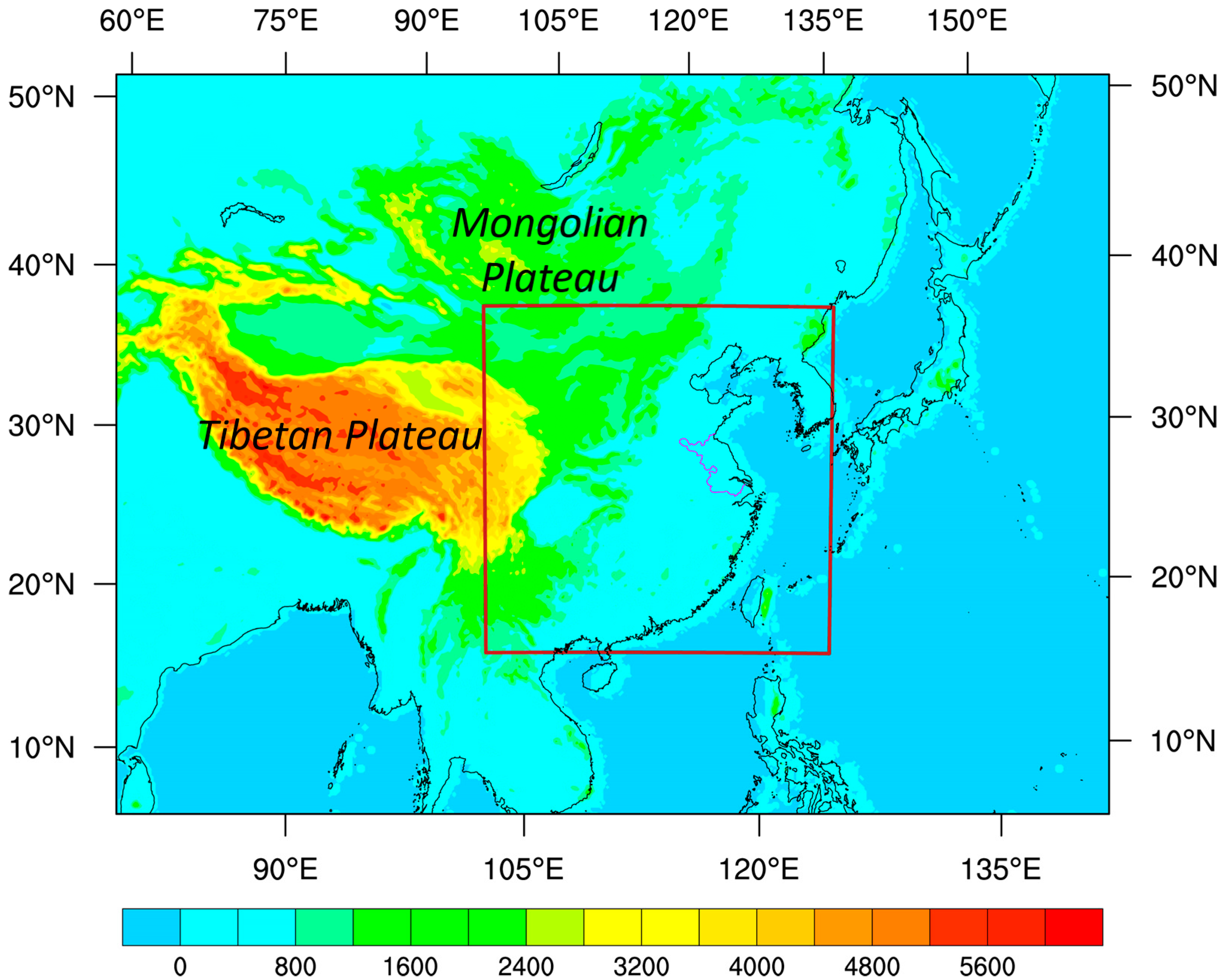
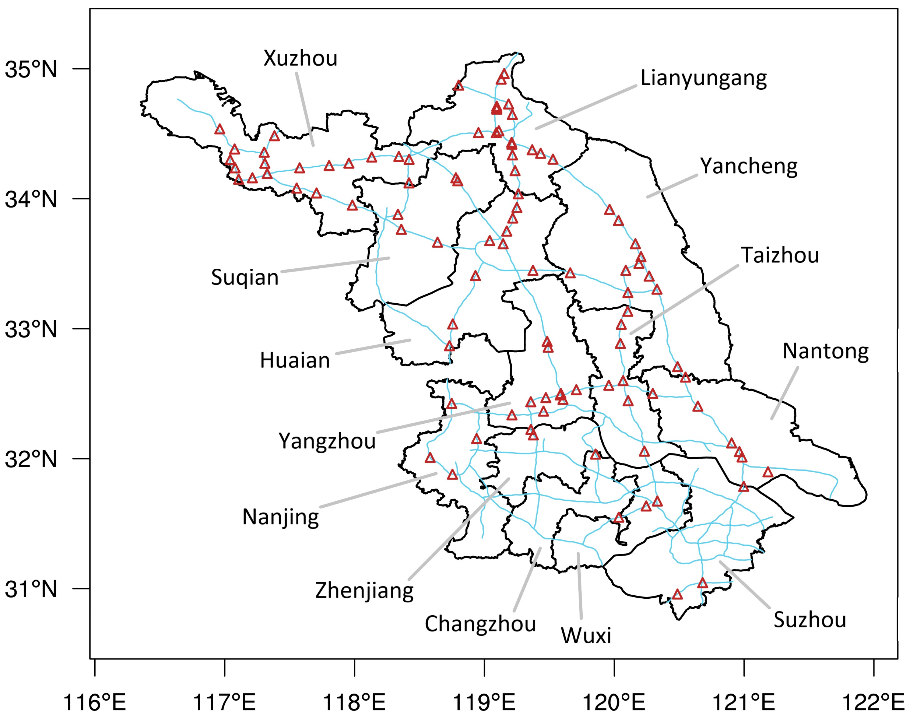
2.1. Data
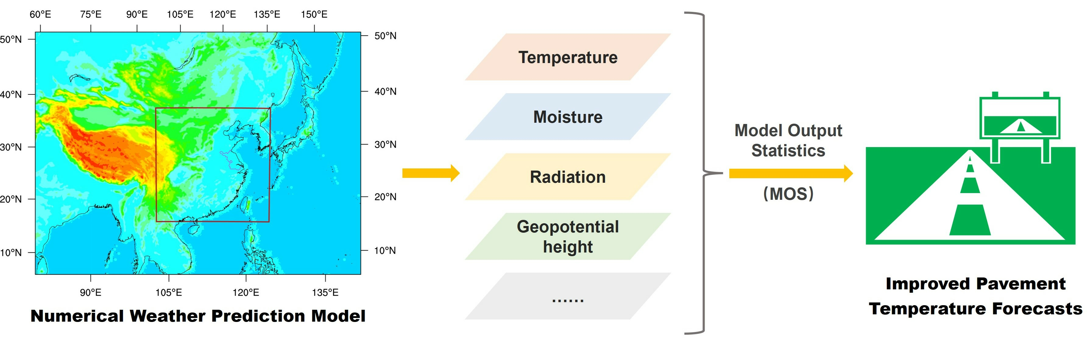
2.2. Methods
2.2.1. Pavement Temperature Forecasts
2.2.2. Verification Metrics
2.2.3. Predictor Importance Analysis
3. Results
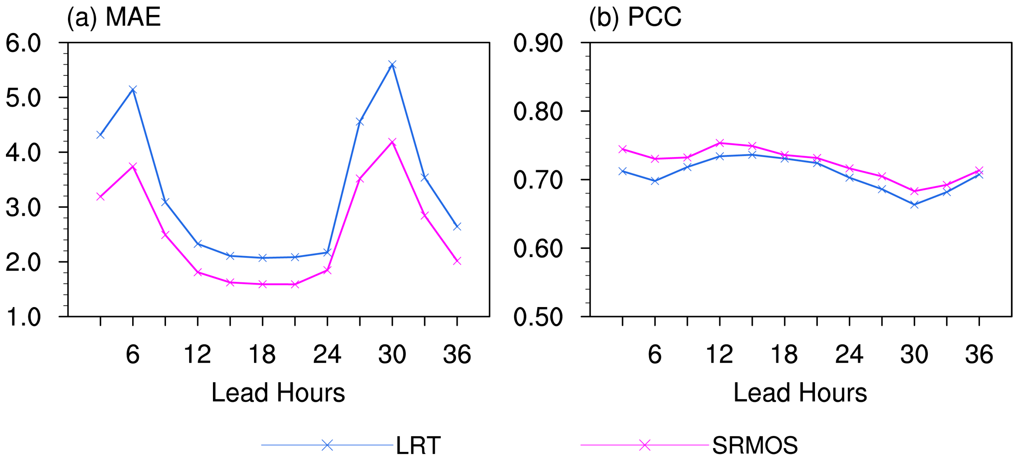
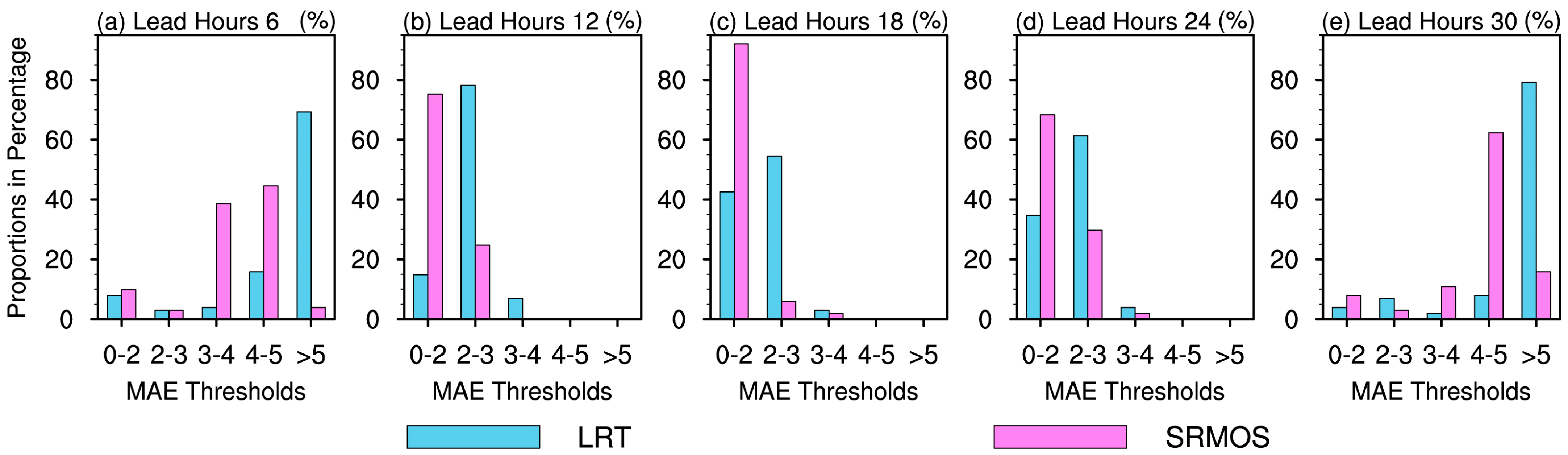
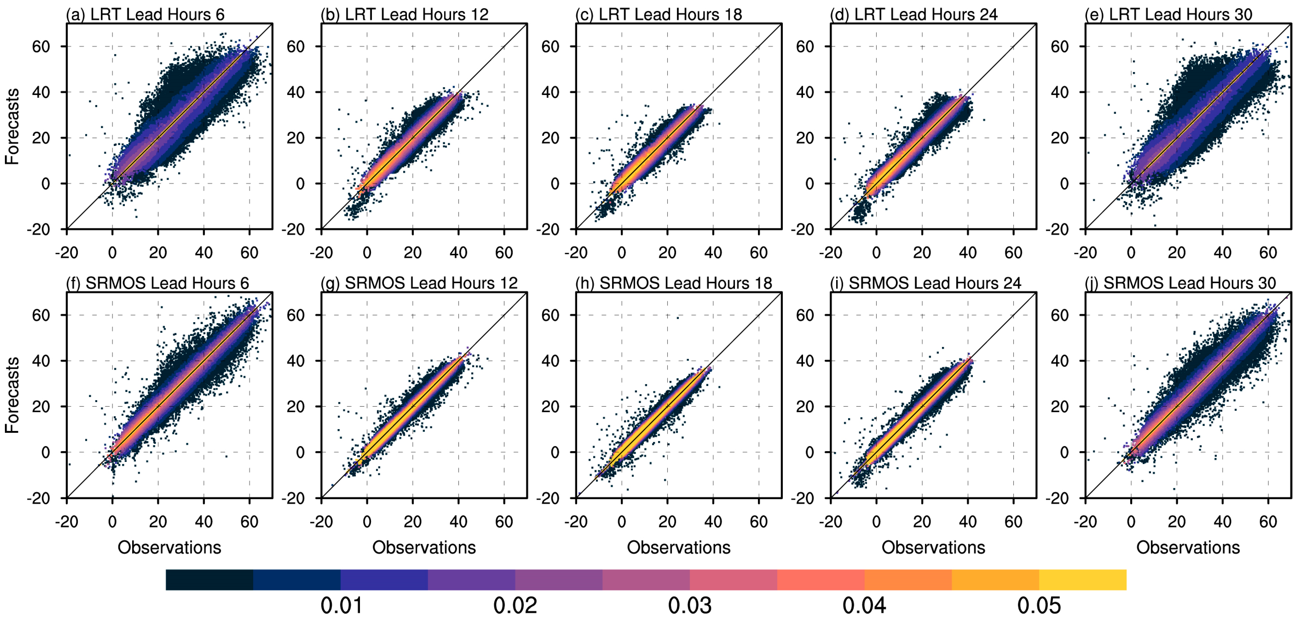
3.1. General Evaluations
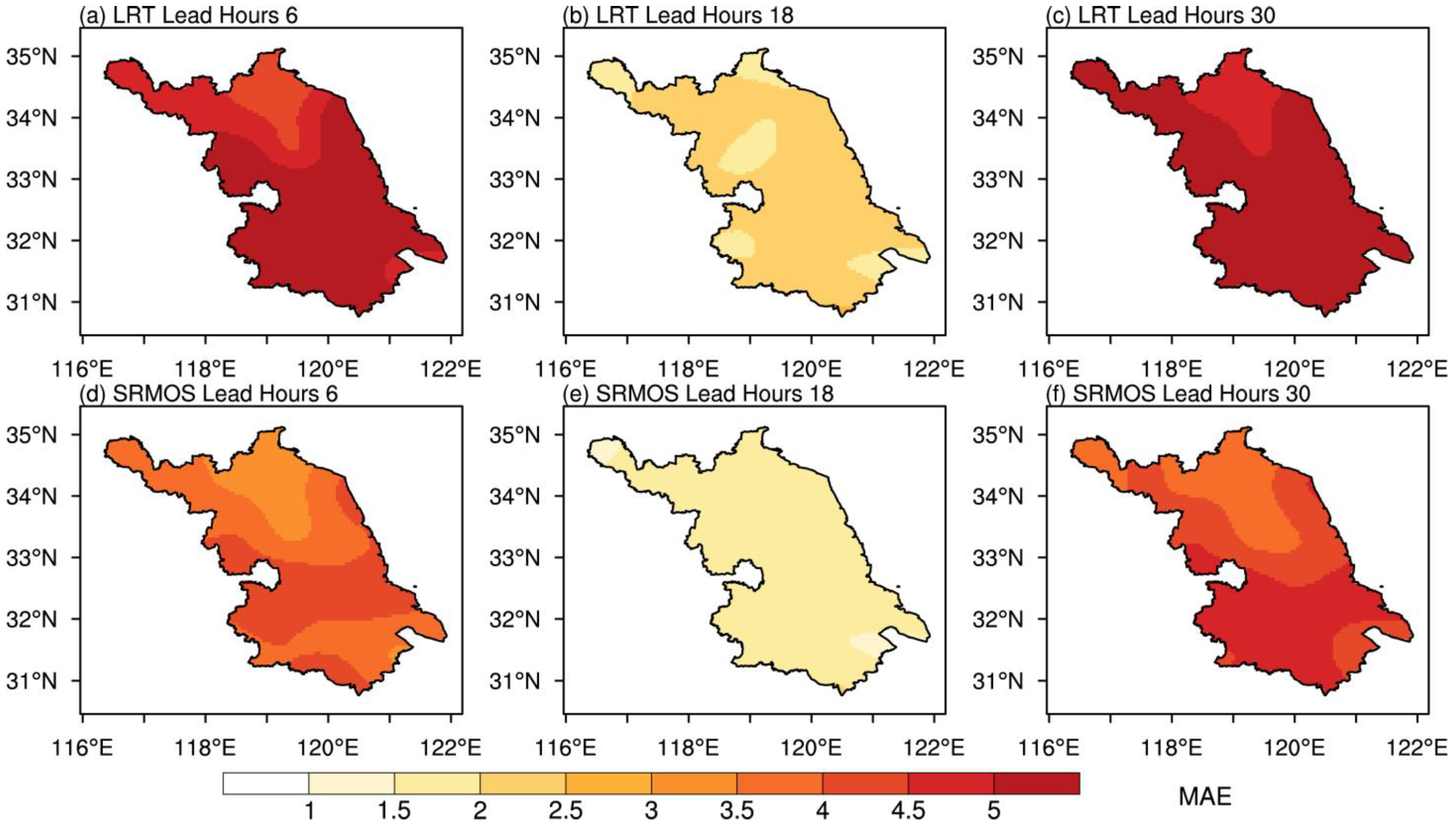
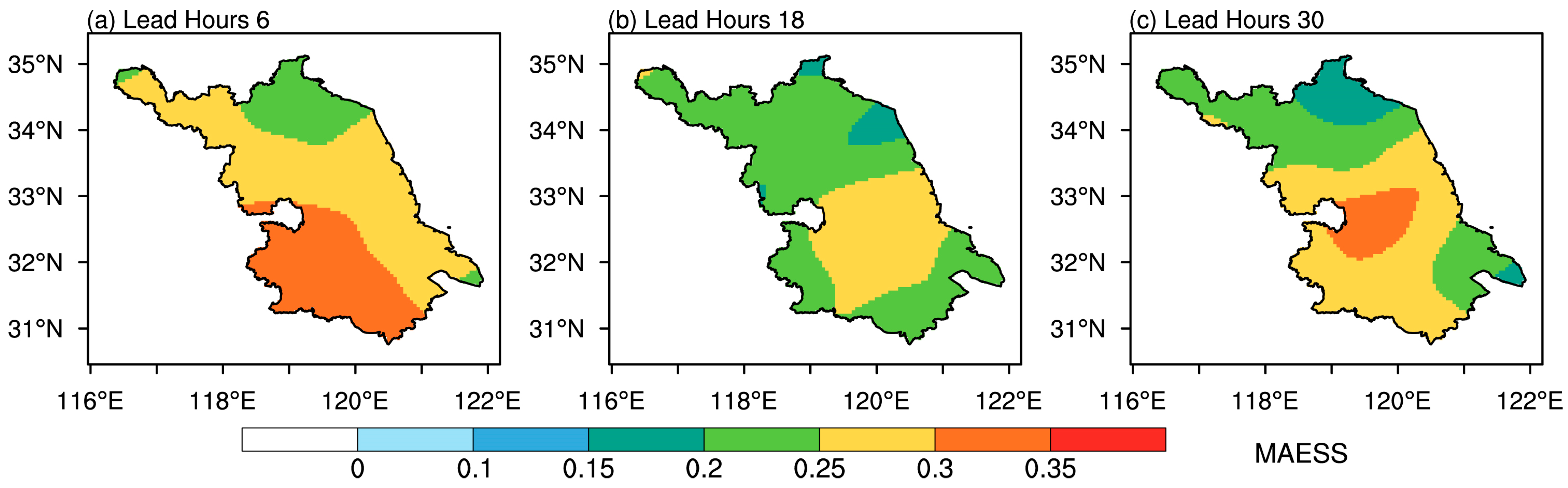
3.2. Details of the Forecast Biases
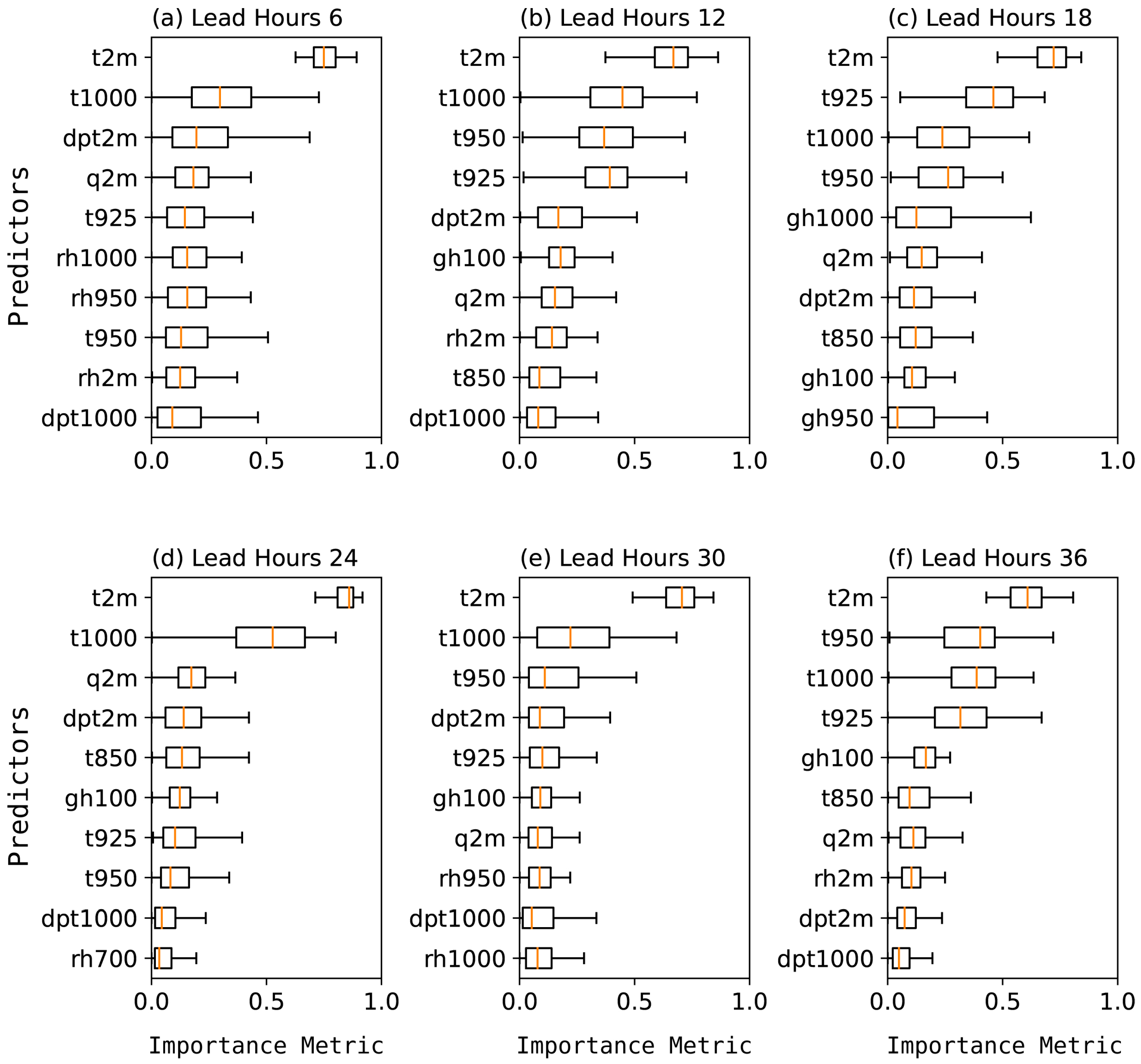
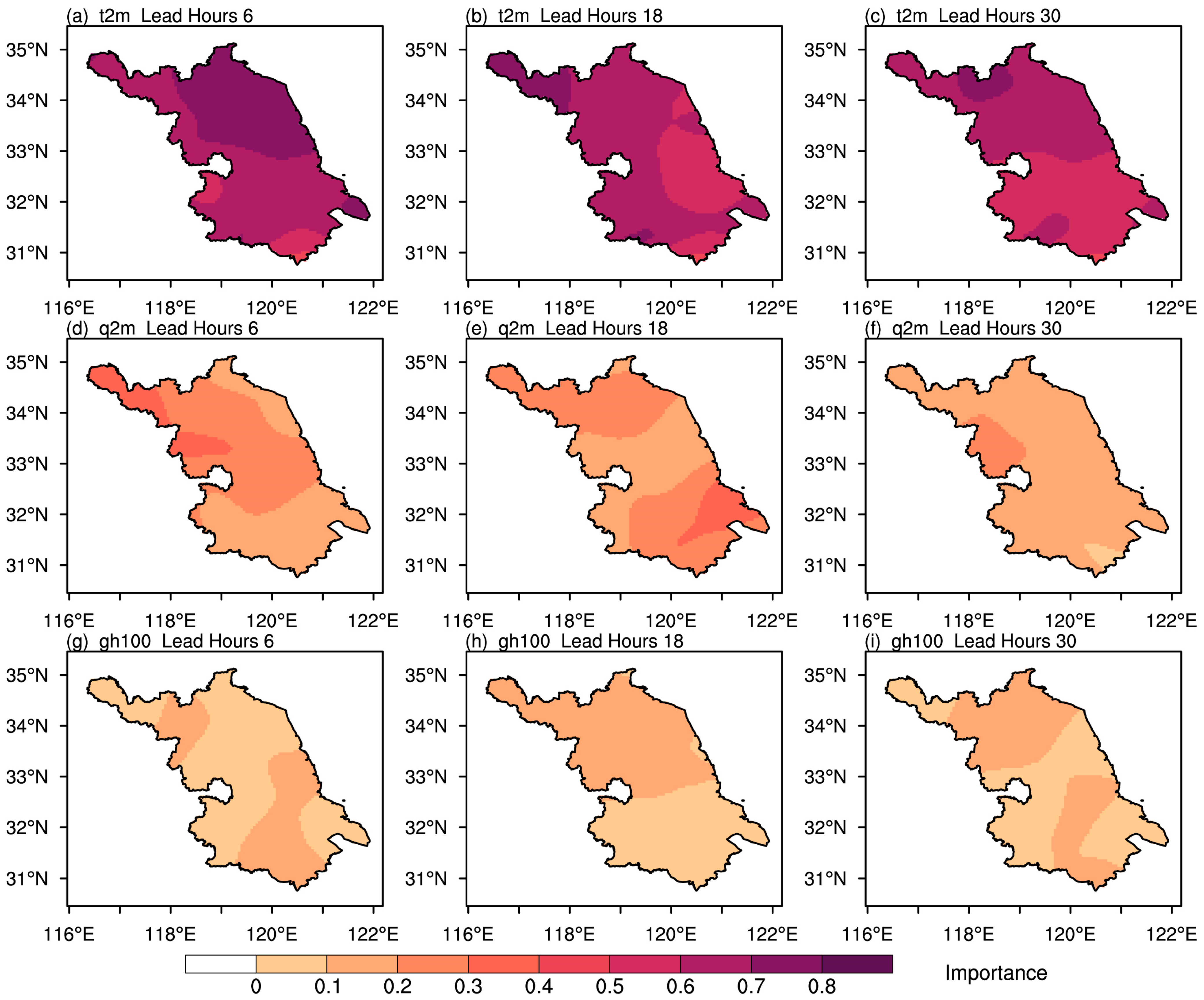
3.3. Predictor Importance Analysis
4. Conclusions
5. Discussion
Author Contributions
Funding
Data Availability Statement
Acknowledgments
Conflicts of Interest
References
- Zhu, S.P.; Ge, F.; Fan, Y.; Zhang, L.; Sielmann, F.; Fraedrich, K.; Zhi, X.F. Conspicuous temperature extremes over Southeast Asia: Seasonal variations under 1.5 degrees C and 2 degrees C global warming. Clim. Change 2020, 160, 343–360. [Google Scholar] [CrossRef]
- Yan, Y.; Wang, H.; Li, G.; Xia, J.; Ge, F.; Zeng, Q.; Ren, X.; Tan, L. Projection of Future Extreme Precipitation in China Based on the CMIP6 from a Machine Learning Perspective. Remote Sens. 2022, 14, 4033. [Google Scholar] [CrossRef]
- You, Q.L.; Chen, D.L.; Wu, F.Y.; Pepin, N.; Cai, Z.Y.; Ahrens, B.; Jiang, Z.H.; Wu, Z.W.; Kang, S.C.; AghaKouchak, A. Elevation dependent warming over the Tibetan Plateau: Patterns, mechanisms and perspectives. Earth Sci. Rev. 2020, 210, 103349. [Google Scholar] [CrossRef]
- Sun, X.R.; Ge, F.; Fan, Y.; Zhu, S.P.; Chen, Q.L. Will population exposure to heat extremes intensify over Southeast Asia in a warmer world? Environ. Res. Lett. 2022, 17, 044006. [Google Scholar] [CrossRef]
- Zhu, S.P.; Yang, H.D.; Liu, D.Y.; Wang, H.B.; Zhou, L.Y.; Zhu, C.Y.; Zu, F.; Wu, H.; Lyu, Y.; Xia, Y.; et al. Observations and Forecasts of Urban Transportation Meteorology in China: A Review. Atmosphere 2022, 13, 1823. [Google Scholar] [CrossRef]
- Zhu, S.P.; Zhi, X.F.; Ge, F.; Fan, Y.; Zhang, L.; Gao, J.Y. Subseasonal Forecast of Surface Air Temperature Using Superensemble Approaches: Experiments over Northeast Asia for 2018. Weather Forecast. 2021, 36, 39–51. [Google Scholar] [CrossRef]
- Pisano, P.; Goodwin, L.; Stern, A. Surface transportation safety and operations: The impacts of weather within the context of climate change. In Proceedings of the Potential Impacts of Climate Change on Transportation Workshop, US Department of Transportation: Centre for Climate Change and Environmental Forecasting, Washington, DC, USA, 1–2 October 2002. [Google Scholar]
- Kim, Y.-J.; Kim, B.-J.; Shin, Y.-S.; Kim, H.-W.; Kim, G.-T.; Kim, S.-J. A case study of environmental characteristics on urban road-surface and air temperatures during heat-wave days in Seoul. Atmos. Ocean. Sci. Lett. 2019, 12, 261–269. [Google Scholar] [CrossRef] [Green Version]
- Androjić, I.; Marović, I. Analysis of influential factors on heat accumulation in structural elements of road underpasses. Sol. Energy 2017, 155, 25–34. [Google Scholar] [CrossRef]
- Dey, K.C.; Mishra, A.; Chowdhury, M. Potential of Intelligent Transportation Systems in Mitigating Adverse Weather Impacts on Road Mobility: A Review. IEEE Trans. Intell. Transp. Syst. 2015, 16, 1107–1119. [Google Scholar] [CrossRef]
- Douglas, E.; Jacobs, J.; Hayhoe, K.; Silka, L.; Daniel, J.; Collins, M.; Alipour, A.; Anderson, B.; Hebson, C.; Mecray, E.; et al. Progress and Challenges in Incorporating Climate Change Information into Transportation Research and Design. J. Infrastruct. Syst. 2017, 23, 9. [Google Scholar] [CrossRef] [Green Version]
- Crevier, L.-P.; Delage, Y. METRo: A New Model for Road-Condition Forecasting in Canada. J. Appl. Meteorol. 2001, 40, 2026–2037. [Google Scholar] [CrossRef]
- Chen, J.; Wang, H.; Xie, P. Pavement temperature prediction: Theoretical models and critical affecting factors. Appl. Therm. Eng. 2019, 158, 113755. [Google Scholar] [CrossRef]
- Adwan, I.; Milad, A.; Memon, Z.A.; Widyatmoko, I.; Ahmat Zanuri, N.; Memon, N.A.; Yusoff, N.I.M. Asphalt Pavement Temperature Prediction Models: A Review. Appl. Sci. 2021, 11, 3794. [Google Scholar]
- Herb, W.; Velasquez, R.; Stefan, H.; Marasteanu, M.O.; Clyne, T. Simulation and Characterization of Asphalt Pavement Temperatures. Road Mater. Pavement Des. 2009, 10, 233–247. [Google Scholar] [CrossRef] [Green Version]
- Chao, J.; Jinxi, Z. Prediction Model for Asphalt Pavement Temperature in High-Temperature Season in Beijing. Adv. Civ. Eng. 2018, 2018, 1837952. [Google Scholar] [CrossRef] [Green Version]
- Wang, T.-h.; Su, L.-j.; Zhai, J.-y. A case study on diurnal and seasonal variation in pavement temperature. Int. J. Pavement Eng. 2014, 15, 402–408. [Google Scholar] [CrossRef]
- Resler, J.; Krč, P.; Belda, M.; Juruš, P.; Benešová, N.; Lopata, J.; Vlček, O.; Damašková, D.; Eben, K.; Derbek, P.; et al. PALM-USM v1.0: A new urban surface model integrated into the PALM large-eddy simulation model. Geosci. Model Dev. 2017, 10, 3635–3659. [Google Scholar] [CrossRef] [Green Version]
- Milad, A.A.; Adwan, I.; Majeed, S.A.; Memon, Z.A.; Bilema, M.; Omar, H.A.; Abdolrasol, M.G.M.; Usman, A.; Yusoff, N.I.M. Development of a Hybrid Machine Learning Model for Asphalt Pavement Temperature Prediction. IEEE Access 2021, 9, 158041–158056. [Google Scholar] [CrossRef]
- Tabrizi, S.E.; Xiao, K.; Van Griensven Thé, J.; Saad, M.; Farghaly, H.; Yang, S.X.; Gharabaghi, B. Hourly road pavement surface temperature forecasting using deep learning models. J. Hydrol. 2021, 603, 126877. [Google Scholar] [CrossRef]
- Wilks, D.S.; Vannitsem, S. Chapter 1—Uncertain Forecasts From Deterministic Dynamics. In Statistical Postprocessing of Ensemble Forecasts; Vannitsem, S., Wilks, D.S., Messner, J.W., Eds.; Elsevier: Amsterdam, The Netherlands, 2018; pp. 1–13. [Google Scholar] [CrossRef]
- Skamarock, C.; Klemp, B.; Dudhia, J.; Gill, O.; Barker, D.M.; Duda, G.; Huang, X.; Wang, W.; Powers, G. A Description of the Advanced Research WRF Version 3. NCAR Tech. Note 2008, 475, 113. [Google Scholar]
- Zhang, L.; Song, L.X.; Zhu, S.P.; Guo, Z.; Wang, H.B.; Zhou, L.Y.; Chen, C.H.; Zhi, X.F. Forecasts of the Warm-Sector Heavy Rainfall With a Warm Shear Pattern Over Coastal Areas of the Yangtze-Huaihe River in a Regional Business Forecast Model. Front. Earth Sci. 2022, 10, 938336. [Google Scholar] [CrossRef]
- Lorenz, E.N. Deterministic Nonperiodic Flow. J. Atmos. Sci. 1963, 20, 130–141. [Google Scholar] [CrossRef]
- LORENZ, E.N. The predictability of a flow which possesses many scales of motion. Tellus 1969, 21, 289–307. [Google Scholar] [CrossRef]
- Slingo, J.; Palmer, T. Uncertainty in weather and climate prediction. Philos. Trans. R. Soc. A-Math. Phys. Eng. Sci. 2011, 369, 4751–4767. [Google Scholar] [CrossRef]
- Zhu, Y.J.; Zhou, X.Q.; Pena, M.; Li, W.; Melhauser, C.; Hou, D.C. Impact of Sea Surface Temperature Forcing on Weeks 3 and 4 Forecast Skill in the NCEP Global Ensemble Forecasting System. Weather Forecast. 2017, 32, 2159–2174. [Google Scholar] [CrossRef]
- Krishnamurti, T.N.; Kishtawal, C.M.; Zhang, Z.; LaRow, T.; Bachiochi, D.; Williford, E.; Gadgil, S.; Surendran, S. Multimodel Ensemble Forecasts for Weather and Seasonal Climate. J. Clim. 2000, 13, 4196–4216. [Google Scholar] [CrossRef]
- Vannitsem, S.; Bremnes, J.B.; Demaeyer, J.; Evans, G.R.; Flowerdew, J.; Hemri, S.; Lerch, S.; Roberts, N.; Theis, S.; Atencia, A.; et al. Statistical Postprocessing for Weather Forecasts: Review, Challenges, and Avenues in a Big Data World. Bull. Amer. Meteorol. Soc. 2021, 102, E681–E699. [Google Scholar] [CrossRef]
- Hamill, T.M. Chapter 7—Practical Aspects of Statistical Postprocessing. In Statistical Postprocessing of Ensemble Forecasts; Vannitsem, S., Wilks, D.S., Messner, J.W., Eds.; Elsevier: Amsterdam, The Netherlands, 2018; pp. 187–217. [Google Scholar] [CrossRef]
- Feng, J.; Zhang, J.; Toth, Z.; Peña, M.; Ravela, S. A New Measure of Ensemble Central Tendency. Weather Forecast. 2020, 35, 879–889. [Google Scholar] [CrossRef]
- Klein, W.H.; Lewis, B.M.; Enger, I. Objective prediction of five-day mean temperatures during winter. J. Atmos. Sci. 1959, 16, 672–682. [Google Scholar] [CrossRef]
- Glahn, H.R.; Lowry, D.A. The Use of Model Output Statistics (MOS) in Objective Weather Forecasting. J. Appl. Meteorol. Climatol. 1972, 11, 1203–1211. [Google Scholar] [CrossRef]
- Vannitsem, S. Dynamical Properties of MOS Forecasts: Analysis of the ECMWF Operational Forecasting System. Weather Forecast. 2008, 23, 1032–1043. [Google Scholar] [CrossRef]
- Li, W.T.; Duan, Q.Y.; Wang, Q.J. Factors Influencing the Performance of Regression-Based Statistical Postprocessing Models for Short-Term Precipitation Forecasts. Weather Forecast. 2019, 34, 2067–2084. [Google Scholar] [CrossRef]
- Sokol, Z.; Bliznak, V.; Sedlak, P.; Zacharov, P.; Pesice, P.; Skuthan, M. Ensemble forecasts of road surface temperatures. Atmos. Res. 2017, 187, 33–41. [Google Scholar] [CrossRef]
- Yang, Y.; Turner, R.; Carey-Smith, T.; Uddstrom, M. A comparison of three model output statistics approaches for the bias correction of simulated soil moisture. Meteorol. Appl. 2020, 27, 15. [Google Scholar] [CrossRef]
- Pinson, P.; Messner, J.W. Chapter 9—Application of Postprocessing for Renewable Energy. In Statistical Postprocessing of Ensemble Forecasts; Vannitsem, S., Wilks, D.S., Messner, J.W., Eds.; Elsevier: Amsterdam, The Netherlands, 2018; pp. 241–266. [Google Scholar] [CrossRef]
- Li, X.; Zeng, M.; Wang, Y.; Wang, W.; Wu, H.; Mei, H. Evaluation of two momentum control variable schemes and their impact on the variational assimilation of radarwind data: Case study of a squall line. Adv. Atmos. Sci. 2016, 33, 1143–1157. [Google Scholar] [CrossRef]
- Li, X.; Zou, X.; Zeng, M. An Alternative Bias Correction Scheme for CrIS Data Assimilation in a Regional Model. Mon. Weather Rev. 2019, 147, 809–839. [Google Scholar] [CrossRef]
- Song-You, H.; Jeong-Ock Jade, L. The WRF Single-Moment 6-Class Microphysics Scheme (WSM6). Asia-Pac. J. Atmos. Sci. 2006, 42, 129–151. [Google Scholar]
- Monin, A.S.; Obukhov, A.M. Basic laws of turbulent mixing in the surface layer of the atmosphere. Tr. Akad. Nauk SSSR Geophiz. Inst. 1954, 24, 163–187. [Google Scholar]
- Chen, F.; Dudhia, J. Coupling an Advanced Land Surface–Hydrology Model with the Penn State–NCAR MM5 Modeling System. Part I: Model Implementation and Sensitivity. Mon. Weather Rev. 2001, 129, 569–585. [Google Scholar] [CrossRef]
- Hong, S.-Y.; Noh, Y.; Dudhia, J. A New Vertical Diffusion Package with an Explicit Treatment of Entrainment Processes. Mon. Weather Rev. 2006, 134, 2318–2341. [Google Scholar] [CrossRef] [Green Version]
- Mlawer, E.J.; Taubman, S.J.; Brown, P.D.; Iacono, M.J.; Clough, S.A. Radiative transfer for inhomogeneous atmospheres: RRTM, a validated correlated-k model for the longwave. J. Geophys. Res. Atmos. 1997, 102, 16663–16682. [Google Scholar] [CrossRef] [Green Version]
- Dudhia, J. Numerical Study of Convection Observed during the Winter Monsoon Experiment Using a Mesoscale Two-Dimensional Model. J. Atmos. Sci. 1989, 46, 3077–3107. [Google Scholar] [CrossRef]
- Kain, J.S.; Fritsch, J.M. The role of the convective “trigger function” in numerical forecasts of mesoscale convective systems. Meteorol. Atmos. Phys. 1992, 49, 93–106. [Google Scholar] [CrossRef]
- Kain, J.S. The Kain–Fritsch Convective Parameterization: An Update. J. Appl. Meteorol. 2004, 43, 170–181. [Google Scholar] [CrossRef]
- Ewan, L.; Al-Kaisy, A.; Veneziano, D. Remote Sensing of Weather and Road Surface Conditions:Is Technology Mature for Reliable Intelligent Transportation Systems Applications? Transp. Res. Rec. 2013, 2329, 8–16. [Google Scholar] [CrossRef] [Green Version]
- Navalgund, R.R.; Jayaraman, V.; Roy, P.S. Remote sensing applications: An overview. Curr. Sci. 2007, 93, 1747–1766. [Google Scholar]
- Friederichs, P.; Wahl, S.; Buschow, S. Chapter 5—Postprocessing for Extreme Events. In Statistical Postprocessing of Ensemble Forecasts; Vannitsem, S., Wilks, D.S., Messner, J.W., Eds.; Elsevier: Amsterdam, The Netherlands, 2018; pp. 127–154. [Google Scholar] [CrossRef]
- Gao, L.; Schulz, K.; Bernhardt, M. Statistical Downscaling of ERA-Interim Forecast Precipitation Data in Complex Terrain Using LASSO Algorithm. Adv. Meteorol. 2014, 2014, 472741. [Google Scholar] [CrossRef] [Green Version]
- Hu, X.; Wang, M.; Liu, K.; Gong, D.; Kantz, H. Using Climate Factors to Estimate Flood Economic Loss Risk. Int. J. Disaster Risk Sci. 2021, 12, 731–744. [Google Scholar] [CrossRef]
- Feng, L.; Wang, X.; He, X.; Gao, J. Fine forecast of high road temperature along jiangsu highways based on INCA system and METRo model. J. Appl. Meteorol. Sci. 2017, 28, 109–118. [Google Scholar]
- Zhang, H.B.; Zhi, X.F.; Chen, J.; Wang, Y.N.; Wang, Y. Study of the modification of multi-model ensemble schemes for tropical cyclone forecasts. J. Trop. Meteorol. 2015, 21, 389–399. [Google Scholar]
- Breiman, L. Random Forests. Mach. Learn. 2001, 45, 5–32. [Google Scholar] [CrossRef] [Green Version]
- Kuhn, M.; Johnson, K. Measuring Predictor Importance. In Applied Predictive Modeling; Kuhn, M., Johnson, K., Eds.; Springer: New York, NY, USA, 2013; pp. 463–485. [Google Scholar] [CrossRef]
- Yan, X.; Wang, X.; Da, X.; Zhao, F.; Niu, X. Variation Characteristics of Expressway Pavement Temperature and Forecast Model in Mountainous Area of Gansu. J. Arid. Meteorol. 2018, 36, 864–872. [Google Scholar]
- Lyu, Y.; Zhi, X.F.; Zhu, S.P.; Fan, Y.; Pan, M.T. Statistical Calibrations of Surface Air Temperature Forecasts over East Asia Using Pattern Projection Methods. Weather. Forecast. 2021, 36, 1661–1674. [Google Scholar] [CrossRef]
- Zhu, S.; Zhang, L.; Jiang, H.; Lyu, Y.; Fan, Y.; Guo, Z.; Zhi, X. Pattern projection calibrations on subseasonal forecasts of surface air temperature over East Asia. Weather. Forecast. 2023, 38, 865–878. [Google Scholar] [CrossRef]
- Najafi, R.; Kermani, M.R.H. Uncertainty Modeling of Statistical Downscaling to Assess Climate Change Impacts on Temperature and Precipitation. Water Resour. Manag. 2017, 31, 1843–1858. [Google Scholar] [CrossRef]
- Zamora, R.J.; Dutton, E.G.; Trainer, M.; McKeen, S.A.; Wilczak, J.M.; Hou, Y.T. The accuracy of solar irradiance calculations used in mesoscale numerical weather prediction. Mon. Weather Rev. 2005, 133, 783–792. [Google Scholar] [CrossRef]
- Yang, D.Z.; Jirutitijaroen, P.; Walsh, W.M. Hourly solar irradiance time series forecasting using cloud cover index. Sol. Energy 2012, 86, 3531–3543. [Google Scholar] [CrossRef]
- Hannak, L.; Knippertz, P.; Fink, A.H.; Kniffka, A.; Pante, G. Why Do Global Climate Models Struggle to Represent Low-Level Clouds in the West African Summer Monsoon? J. Clim. 2017, 30, 1665–1687. [Google Scholar] [CrossRef]
- Phakula, S.; Landman, W.A.; Engelbrecht, C.J.; Makgoale, T. Forecast Skill of Minimum and Maximum Temperatures on Subseasonal-to-Seasonal Timescales Over South Africa. Earth Space Sci. 2020, 7, 11. [Google Scholar] [CrossRef] [Green Version]
- Srivastava, P.; Sharan, M.; Kumar, M. A note on surface layer parameterizations in the weather research and forecast model. Dyn. Atmos. Oceans 2021, 96, 10. [Google Scholar] [CrossRef]
- Hamill, T.M.; Whitaker, J.S. Ensemble Calibration of 500-hPa Geopotential Height and 850-hPa and 2-m Temperatures Using Reforecasts. Mon. Weather Rev. 2007, 135, 3273–3280. [Google Scholar] [CrossRef] [Green Version]
- Zhi, X.; Qi, H.; Bai, Y.; Lin, C. A comparison of three kinds of multimodel ensemble forecast techniques based on the TIGGE data. Acta Meteorol. Sin. 2012, 26, 41–51. [Google Scholar] [CrossRef]
- Ji, L.; Zhi, X.; Schalge, B.; Stephan, K.; Wu, Z.; Wu, C.; Simmer, C.; Zhu, S. Dynamic downscaling ensemble forecast of an extreme rainstorm event in South China by COSMO EPS. Front. Earth Sci. 2022, 10, 969742. [Google Scholar] [CrossRef]
- Zhu, Y.; Zhi, X.; Lyu, Y.; Zhu, S.; Tong, H.; Mamtimin, A.; Zhang, H.; Huo, W. Forecast calibrations of surface air temperature over Xinjiang based on U-net neural network. Front. Environ. Sci. 2022, 10, 11321. [Google Scholar] [CrossRef]
- Zhang, J.; Feng, J.; Li, H.; Zhu, Y.; Zhi, X.; Zhang, F. Unified Ensemble Mean Forecasting of Tropical Cyclones Based on the Feature-Oriented Mean Method. Weather. Forecast. 2021, 36, 1945–1959. [Google Scholar] [CrossRef]
- Ji, L.; Zhi, X.; Zhu, S.; Fraedrich, K. Probabilistic Precipitation Forecasting over East Asia Using Bayesian Model Averaging. Weather. Forecast. 2019, 34, 377–392. [Google Scholar] [CrossRef]
- Lyu, Y.; Zhi, X.; Wu, H.; Zhou, H.; Kong, D.; Zhu, S.; Zhang, Y.; Hao, C. Analyses on the Multimodel Wind Forecasts and Error Decompositions over North China. Atmosphere 2022, 13, 1652. [Google Scholar]
- Schnebele, E.; Tanyu, B.F.; Cervone, G.; Waters, N. Review of remote sensing methodologies for pavement management and assessment. Eur. Transp. Res. Rev. 2015, 7, 7. [Google Scholar] [CrossRef] [Green Version]
- Capozzi, V.; Mazzarella, V.; Vivo, C.D.; Annella, C.; Greco, A.; Fusco, G.; Budillon, G. A Network of X-Band Meteorological Radars to Support the Motorway System (Campania Region Meteorological Radar Network Project). Remote Sens. 2022, 14, 2221. [Google Scholar] [CrossRef]
- Song, Y.; Wright, G.; Wu, P.; Thatcher, D.; McHugh, T.; Li, Q.; Li, S.J.; Wang, X. Segment-Based Spatial Analysis for Assessing Road Infrastructure Performance Using Monitoring Observations and Remote Sensing Data. Remote Sens. 2018, 10, 1696. [Google Scholar]


| Physics | Scheme |
|---|---|
| Microphysics | WRF Single-Moment 6-class scheme [41] |
| Surface layer | Monin-Obukhov [42] |
| Land surface | Noah Land Surface Model [43] |
| Planetary boundary layer | Yonsei University scheme [44] |
| Longwave radiation | Rapid Radiative Transfer Model [45] |
| Shortwave radiation | Dudhia scheme [46] |
| Cumulus parameterization | Kain-Fritsch scheme [47,48] |
| Predictor Variables | Abbreviation |
|---|---|
| Temperature at 2 m | t2m |
| Specific humidity | q2m |
| Dew point temperature at 2 m | dpt2m |
| Relative humidity at 2 m | rh2m |
| Temperature at p hPa | tp |
| Geopotential height at p hPa | ghp |
| Relative humidity at p hPa | rhp |
| Dew point temperature at p hPa | dptp |
Disclaimer/Publisher’s Note: The statements, opinions and data contained in all publications are solely those of the individual author(s) and contributor(s) and not of MDPI and/or the editor(s). MDPI and/or the editor(s) disclaim responsibility for any injury to people or property resulting from any ideas, methods, instructions or products referred to in the content. |
© 2023 by the authors. Licensee MDPI, Basel, Switzerland. This article is an open access article distributed under the terms and conditions of the Creative Commons Attribution (CC BY) license (https://creativecommons.org/licenses/by/4.0/).
Share and Cite
Zhu, S.; Lyu, Y.; Wang, H.; Zhou, L.; Zhu, C.; Dong, F.; Fan, Y.; Wu, H.; Zhang, L.; Liu, D.; et al. Pavement Temperature Forecasts Based on Model Output Statistics: Experiments for Highways in Jiangsu, China. Remote Sens. 2023, 15, 3956. https://doi.org/10.3390/rs15163956
Zhu S, Lyu Y, Wang H, Zhou L, Zhu C, Dong F, Fan Y, Wu H, Zhang L, Liu D, et al. Pavement Temperature Forecasts Based on Model Output Statistics: Experiments for Highways in Jiangsu, China. Remote Sensing. 2023; 15(16):3956. https://doi.org/10.3390/rs15163956
Chicago/Turabian StyleZhu, Shoupeng, Yang Lyu, Hongbin Wang, Linyi Zhou, Chengying Zhu, Fu Dong, Yi Fan, Hong Wu, Ling Zhang, Duanyang Liu, and et al. 2023. "Pavement Temperature Forecasts Based on Model Output Statistics: Experiments for Highways in Jiangsu, China" Remote Sensing 15, no. 16: 3956. https://doi.org/10.3390/rs15163956