
D-VINS: Dynamic Adaptive Visual–Inertial SLAM with IMU Prior and Semantic Constraints in Dynamic Scenes
by
 ,
,
Yang Sun
1,
Qing Wang
1,*,
Chao Yan
1,2,
Youyang Feng
1,
Rongxuan Tan
1,
Xiaoqiong Shi
1 and
Xueyan Wang
1 1
School of Instrument Science and Engineering, Southeast University, Nanjing 210096, China
2
School of Electrical Engineering and Automation, Changshu Institute of Technology, Changshu 215500, China
*
Author to whom correspondence should be addressed.
Remote Sens. 2023, 15(15), 3881; https://doi.org/10.3390/rs15153881
Submission received: 26 May 2023
/
Revised: 25 July 2023
/
Accepted: 1 August 2023
/
Published: 4 August 2023
(This article belongs to the Special Issue Machine Vision and Advanced Image Processing in Remote Sensing II)
Abstract
:Visual–inertial SLAM algorithms empower robots to autonomously explore and navigate unknown scenes. However, most existing SLAM systems heavily rely on the assumption of static environments, making them ineffective when confronted with dynamic objects in the real world. To enhance the robustness and localization accuracy of SLAM systems in dynamic scenes, this paper introduces a visual–inertial SLAM framework that integrates semantic and geometric information, called D-VINS. This paper begins by presenting a method for dynamic object classification based on the current motion state of features, enabling the identification of temporary static features within the environment. Subsequently, a feature dynamic check module is devised, which utilizes inertial measurement unit (IMU) prior information and geometric constraints from adjacent frames to calculate dynamic factors. This module also validates the classification outcomes of the temporary static features. Finally, a dynamic adaptive bundle adjustment module is developed, utilizing the dynamic factors of the features to adjust their weights during the nonlinear optimization process. The proposed methodology is evaluated using both public datasets and a dataset created specifically for this study. The experimental results demonstrate that D-VINS stands as one of the most real-time, accurate, and robust systems for dynamic scenes, showcasing its effectiveness in challenging real-world scenes.
1. Introduction
Simultaneous localization and mapping (SLAM) [1] is a crucial technology for advanced robotics applications, enabling collision-free navigation and environment exploration [2]. SLAM heavily relies on the sensors carried by robots to simultaneously achieve high-precision localization and environment mapping. Visual SLAM (VSLAM) [3,4] utilizes cameras to estimate the robot’s position, offering several advantages such as cost-effectiveness, lower energy consumption, and reduced computational requirements. Over the last decade, the VSLAM framework has witnessed rapid development, with notable frameworks such as SOFT2 [5], VINS-Mono [6], ORB-SLAM3 [7], and DM-VIO [8]. Most of these algorithms employ optimization-based methods to construct epipolar constraints, BA, or minimum photometric constraints with features in the environment. VINS-Fusion [9] leverages optical flow to track feature points in the front end and optimizes the minimum reprojection error to solve the poses with BA in the back end. ORB-SLAM2 [10] uses ORB feature points to improve tracking and incorporates a loop closure thread to achieve higher accuracy in global pose estimation. Building upon ORB-SLAM2, ORB-SLAM3 integrates an IMU to enhance the system robustness and stands as one of the most advanced VSLAM solutions to date.
The essence of SLAM pose estimation lies in the robot’s perception of its relative movement in the environment. In terms of the localization aspect of SLAM, the accuracy of pose estimation is greatly affected by the proportion of dynamic feature points being tracked in the field of view. When the proportion of dynamic feature points is relatively small, non-dynamic SLAM algorithms can utilize statistical methods like RANSAC [11] to identify and discard these few dynamic points as outliers. However, when dynamic objects occupy more than half or the majority of the field of view, there are limited static feature points available for tracking. This presents a significant challenge that needs to be addressed using dynamic SLAM algorithms. In such cases, the accuracy of SLAM pose estimation significantly decreases and can even lead to failure, especially for feature-based VSLAM approaches [5,6,7,8]. Consequently, these open-source algorithms often experience a loss in accuracy or even failure when deployed in dynamic environments such as city streets or rural roads with numerous dynamic objects.
To improve the system accuracy and robustness in highly occluded environments, we extend the work of VINS-Fusion and propose a robust dynamic VSLAM framework, called D-VINS. D-VINS proposes a perceptual classification algorithm with missed detection compensation and assigns different weights to feature points during BA based on their geometric constraints. The main contributions of this paper are summarized as follows:
- A feature classification using the YOLOV5 [12] object detection algorithm is proposed in the front end, which divides dynamic feature points into three categories: absolute static points, absolute dynamic points, and temporary static points. Then, the dynamic factors of temporary static features are calculated based on the IMU pre-integration prior constraint and the epipolar constraint. The temporary static features are classified again according to the dynamic factors.
- A robust BA optimization method based on the dynamics factor is proposed in the back end. If the object is more dynamic, its feature weights are decreased, and vice versa.
- Extensive experiments are carried out on public datasets like TUM, KITTI, and VIODE, and our dataset. These datasets include extensive occlusion scenes, and the results from these datasets are representative. The experiment results demonstrate the accuracy and robustness of our proposed D-VINS.
2. Related Work
Dynamic SLAM methods can be classified into two categories: geometry-based methods and semantic-based methods. Geometry-based methods rely on the geometric constraints derived from the inter-frame camera motion, with a potential decrease in the segmentation accuracy. Semantic-based methods leverage deep-learning networks to achieve the highly precise segmentation of known objects. However, the implementation of these methods often requires high-performance computing platforms.
2.1. Geometry-Based Dynamic SLAM
Geometry-based methods rely on geometric constraints between camera frames to eliminate outliers. Dynamic objects can be identified as they deviate from the geometric motion consistency observed between frames. Additionally, statistical analysis allows for the differentiation of inner points (static points) from outliers (dynamic points). Most SLAM systems, like VINS-Mono, use RANSAC with epipolar constraints to remove outliers by calculating the fundamental matrix using the eight-point method. However, RANSAC becomes less effective when outliers dominate the dataset.
DGS-SLAM [13] presents an RGB-D SLAM approach specifically designed for dynamic environments. It addresses outlier impacts during optimization by introducing new robust kernel functions.
DynaVINS [14] introduces a novel loss function that incorporates IMU pre-integration results as priors in BA. In the loop closure detection module, loops from different features are grouped for selective optimization.
PFD-SLAM [15] utilizes GMS (grid-based motion statistics) [16] to ensure accurate matching with RANSAC. Subsequently, it calculates the homography transformation to extract the dynamic region, which is accurately determined using particle filtering.
ClusterSLAM [17] clusters feature points based on motion consistency to reject dynamic objects.
In general, geometry-based methods offer higher accuracy and lower computational costs compared to semantic-based methods. However, they lack the semantic information required for precise segmentation. Moreover, geometry-based methods heavily rely on experience-based hyperparameters, which can significantly limit algorithm feasibility.
2.2. Semantic-Based Dynamic SLAM
Currently, deep-learning networks have achieved remarkable advancements in speed and accuracy in various computer vision tasks, including object detection, semantic segmentation, and optical flow. These networks can provide object detection results, such as bounding boxes, which can be utilized in dynamic SLAM systems. To accurately detect dynamic objects, deep-learning-based methods often incorporate geometric information to capture the real motion state in the current frame.
For example, DynaSLAM [18] is an early dynamic SLAM system that combines multi-view geometry with deep learning. It utilizes MASK R-CNN, which offers pixel-level semantic priors for potential dynamic objects in images.
Dynamic-SLAM [19] detects dynamic objects using the SSD (single shot multi-box detector) [20] object detection network and addresses missed detections by employing a constant velocity motion model. Moreover, it sets a threshold for the average parallax of features within the bounding box area to further reject dynamic features. However, this method’s reliance on bounding boxes may incorrectly reject static feature points belonging to the background.
DS-SLAM [21] employs the SegNet network to eliminate dynamic object features, which are then tracked using the Lucas–Kanade (LK) optical flow algorithm [22]. The fundamental matrix is calculated using RANSAC. The distance between the matched points and their epipolar line is computed, and, if the distance exceeds a certain threshold, the point is considered dynamic and subsequently removed. Additionally, depth information from RGB-D cameras is often employed for dynamic object detection.
RS-SLAM [23] detects dynamic features with semantic segmentation, and a Bayesian update method based on the previous segmentation results is used to refine the current coarse segmentation. It also utilizes depth images to compute the Euclidean distance between such two movable regions.
Dynamic-VINS [24] proposes an RGB-D-based visual–inertial odometry approach specifically designed for embedded platforms. It reduces the computational burden by employing grid-based feature detection algorithms. Semantic labels and the depth information of dynamic features are combined to separate the foreground and background. A moving consistency check based on IMU pre-integration is introduced to address missed detection issues.
YOLO-SLAM [25] is an RGB-D SLAM system that obtains an object’s semantic labels using Darknet19-YOLOv3. The drawback is that it cannot be run in real time.
SG-SLAM [26] is a real-time RGB-D SLAM system that adds a dynamic object detection thread and semantic mapping thread based on ORB-SLAM2 for creating global static 3D reconstruction maps.
In general, geometry-based methods offer faster processing times but lack semantic information. In contrast, deep-learning-based methods excel in dynamic object detection by detecting potential dynamic objects with semantic information. However, it is challenging to run deep-learning algorithms in real time on embedded platforms. Their accuracy heavily relies on the training results. Moreover, most of these methods use RGB-D cameras, which tightly couple geometric and depth information, making them more suitable for indoor environments. Few algorithms are specifically designed for outdoor dynamic scenes.
Although current dynamic SLAM methods can detect dynamic objects, they often oversimplify their treatment, limited to either discarding or preserving them. Additionally, challenges arise when the camera is heavily obscured by moving objects. To address these limitations, we propose a dynamic SLAM method that integrates both geometric and semantic information, tightly incorporating IMU prior constraints into the dynamic feature check and optimization process.
3. Methods
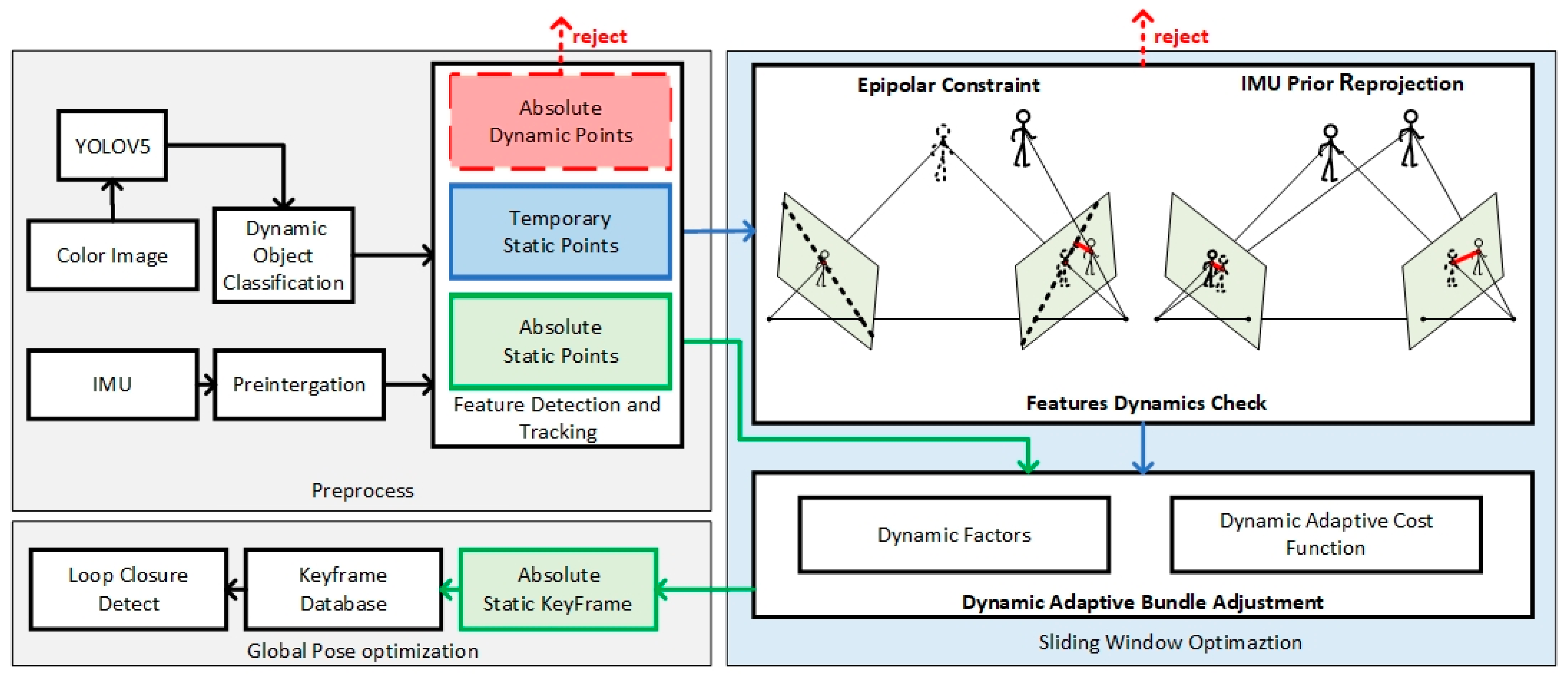
The system is implemented based on VINS-Fusion [9], an optimization-based estimation framework that supports multiple sensors, including stereo, monocular, and IMU sensors. The system initialization follows a loosely coupled approach, where Harris corners are extracted in the front end and tracked using the LK optical flow. In the back end, the system state is marginalized and optimized using a sliding window approach. Figure 1 illustrates the system workflow. For object detection, we utilize the Common Objects in COntext (COCO) dataset, which comprises 80 object categories commonly found in daily life, allowing algorithms trained on this dataset to recognize the majority of objects in everyday scenes.
In dynamic object classification, the color image is initially processed by the fast convolutional neural network You Only Look Once (YOLO) [12], which provides semantic labels of the COCO dataset [27] and bounding boxes of objects. The Harris [28] keypoints are then extracted, and only those points from absolute static objects and temporary static objects are tracked using the LK optical flow in the front end. The IMU sensor provides feature states, like translation, rotation, and velocity with prior motion constraints. The feature’s dynamic factor is determined by the root mean square of the IMU pre-integration error and epipolar constraint. During the feature dynamic check, the dynamic factors of the temporary static points are calculated, indicating the movement of the feature points. A larger numerical value suggests that the feature points are likely to be dynamic. To preserve potential points in dynamic scenes, the feature rejection strategy focuses on retaining points identified by dynamic factors rather than removing all movable points.
In the back end, we propose a novel loss function with adaptive weights based on dynamic factors in BA, a process used to refine camera poses and spatial point positions. The typical approach involves minimizing the reprojection error, which quantifies the difference between landmarks and their observed pixels in the image. To optimize the cost function, feature weights are incorporated as parameters. D-VINS divides the conventional optimization process into two steps. Firstly, the feature weights are fixed to independently optimize the system states. Then, the system states are fixed to optimize the weights. This process is iterated until the required number of iterations is reached, or until the weights converge. Additionally, dynamic factors are introduced to adjust the feature weights.
3.1. Dynamic Object Classification
In dynamic environments, tracking static features is crucial for SLAM systems to maintain localization accuracy. However, deep-learning models struggle to clearly define the boundary between dynamic and static objects. For instance, while books are typically considered static objects, they become dynamic when a person holds them, similar to cars in a parking lot or on a highway. Therefore, relying solely on semantic information is insufficient for robots to detect moving objects in such environments.
3.1.1. Semantic Label Incremental Updating with Bayes’ Rule
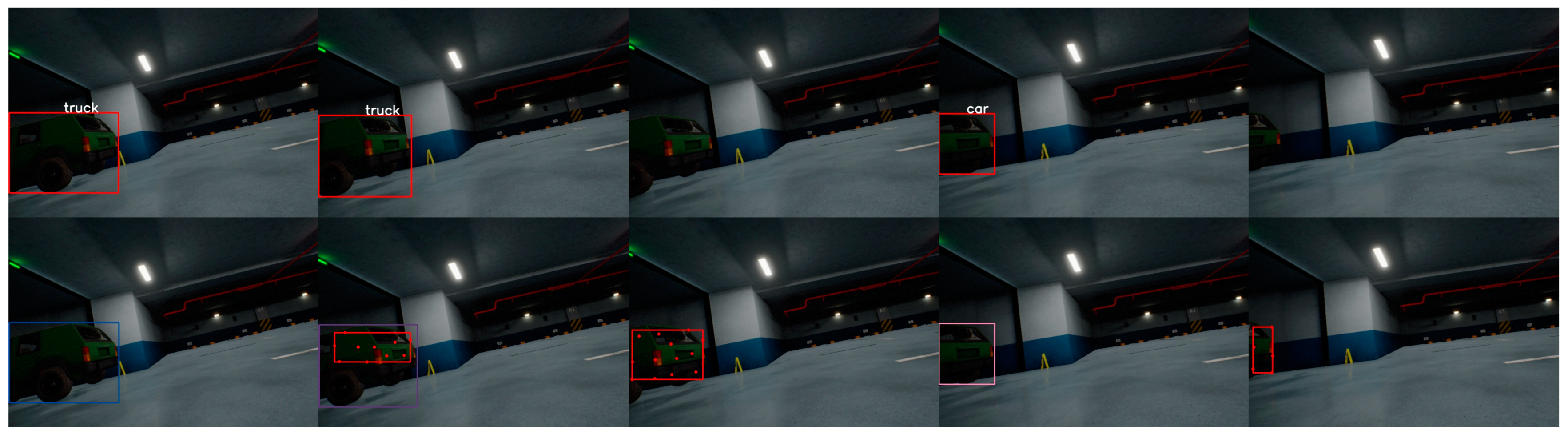
To recognize a wide range of objects, we utilized the COCO dataset to train the YOLOV5 model, which includes 80 common object categories. However, not all objects need to be detected, so we focused on the 17 most common categories. The process involves inputting color images to YOLOV5, accelerated with TensorRT [29], accelerating to obtain semantic labels of the COCO categories. Bounding boxes help approximate the region of dynamic objects in the images, and feature points within these boxes are assigned semantic labels. As the object detection network can sometimes have missing or incorrect detections, D-VINS employs Bayes’ rule to update the feature’s semantic label and mitigate errors in specific frames. This approach transforms the labeling problem into a maximum posterior problem, enhancing the accuracy of semantic labeling.
The th map point in the given world co-ordinates observed in the th frame can be written as . denotes the pixels in camera co-ordinates that correspond to the th map point. The projection process of the feature points is as follows:
whereis the depth of the map points, is the extrinsic matrix, and denotes the transformation matrix from the world co-ordinates to the observation frame. and denote the ground truth of the semantic labels of the th feature points from the beginning frame to the th frame and the measurements of the deep-learning bounding boxes. According to Bayes’ rule, there are
This is a maximum posterior problem, shown as
The semantic labels of feature points in the current frame can be influenced by dynamic objects detected in previous frames. Consequently, the semantic label probability distribution of the th feature point in the th frame is affected by the multi-frame history.
Upon obtaining the semantic information of the current frame, D-VINS checks its consistency with the previous frames. If the previous semantic label matches the one in the current frame, the detection result of the current frame is considered more reliable, and vice versa. The detailed algorithm steps are presented in Algorithm 1.
| Algorithm 1: Semantic label updating with Bayesian rule |
| Input: Current frame bounding box ; current frame’s feature points ; previous frame’s dynamic label ; non-updated current frame’s dynamic label; threshold of the dynamic label; frequency of feature point being observed Output: Current frame’s dynamic label. |
| 1: for each in this Frame do: 2: for each bounding box in this Frame do: 3: if (InThisBoundingBox(,)) && ()) then, 4: ++; 5: ; 6: ; 7: end if 8: end for 9: ; 10: end for |
3.1.2. Feature Point Motion State Classification
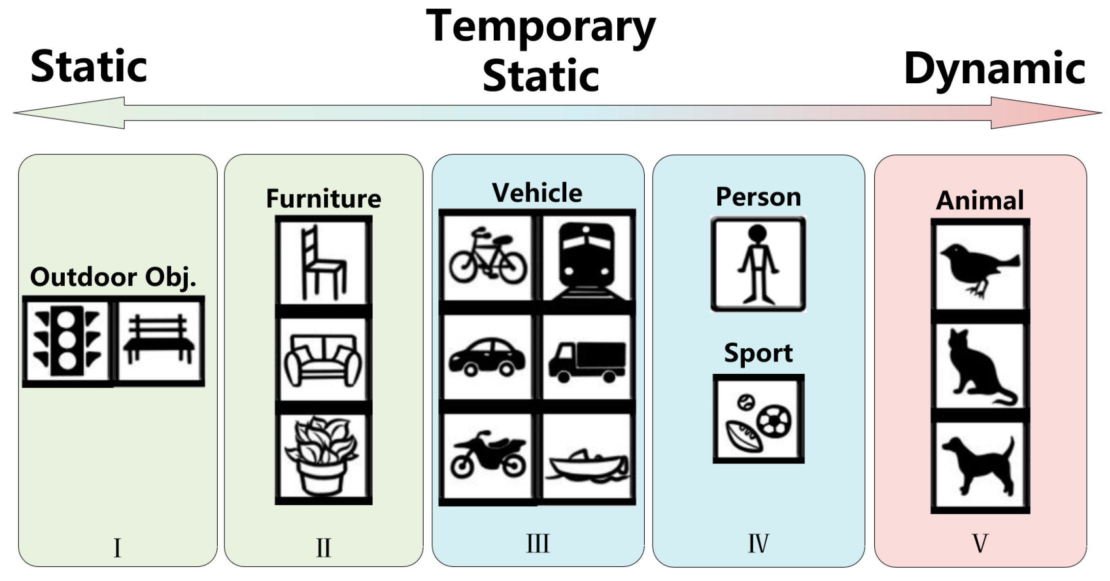
The feature point classification is divided into two parts. The first part is to classify the COCO categories according to the possibility of motion based on life experience. The classification is divided into five levels (I to V), with higher levels indicating a higher possibility of movement. Level I includes public facilities (e.g., traffic light and bench), Level II includes furniture (e.g., chair, sofa, and bed), Level III includes transportation (e.g., bicycle, car, motorbike, bus, truck, and boat), Level IV includes sports (e.g., football and basketball) and people (e.g., person), and Level V includes animals (e.g., cat, dog, and bird), as depicted in Figure 2.
The second part involves dividing feature points into three categories based on their movement in the current frame: absolute stationary points, temporary stationary points, and absolute dynamic points.
Generally, if an object is detected as a bench, sofa, or potted plant, its feature points are likely to be static, making them suitable for pose estimation and mapping. If the semantic label indicates animals such as birds, cats, or dogs, these features are considered dynamic. Animals typically move continuously and occupy a small area in an image, exerting less impact on the SLAM system. As shown in Figure 2, objects of Level I and Level II are classified as absolute static objects, objects of Level III and Level IV are temporary static objects, and objects of Level V are absolute dynamic objects.
3.2. Feature Dynamic Check with IMU Prior and Epipolar Constraints
To check the current motion state of movable objects, D-VINS calculates dynamic factors to find the absolute dynamic points. For temporary static points, the dynamic factors are determined in two steps. Firstly, the IMU pre-integration calculates the initial pose of the current frame, and the reprojection error is obtained by projecting the 3D feature points onto the image plane. Secondly, the foundational matrix is calculated based on epipolar geometry to determine the distance from the feature points to their respective epipolar lines, constituting the second part of the dynamic factor.
If the dynamic factor of a feature point falls below a certain threshold, the point is labeled as an absolute dynamic point.
3.2.1. Dynamic Factor of Reprojection Error Based on IMU Prior Constraint
Conventional visual reprojection involves projecting a feature point from its previous observed frame onto the pixel plane of the current frame. However, the reprojection error cannot be calculated if the camera pose of the current frame is unknown. To address this limitation, IMU pre-integration offers an initial estimate for the current frame’s camera pose, enabling the calculation of the reprojection error and the rejection of dynamic objects using the IMU sensor.
There must be errors between the estimation pose and the real camera pose, which means the reprojection points and the observation points are usually not coincident. For the map point in the world co-ordinates , its pixel co-ordinates projected onto the th frame are . According to Equation (1), a relationship between the map points and pixel points according to the camera projection model exists, as follows:
Equation (5) can be written in matrix form, , and the residual of the reprojection error is as follows:
where is the Lie algebra of the th frame in the body frame, and is the intrinsic matrix obtained via camera calibration [30]. The camera poses of theth frame are obtained via IMU pre-integration:
where , , and are the pre-integration terms of position, velocity, and pose, which change the reference frame from the world frame to the local body frame. , , and are the system states of theth body frame. From Equation (7), the pose of the jth frame is obtained. The pixel co-ordinates in the jth frame projected from the ith frame are . And the observation in theth frame is . Through Equation (6), the new visual reprojection residualof the map point can be established using the camera projection model:
where is the transformation matrix from the body frame to the camera frame, which is obtained using Kalibr [31]. and represent the transformation matrix between IMU frames and the world co-ordinates. and represent the translation matrix between the body frame and world frame. represents the pinhole camera projection model.
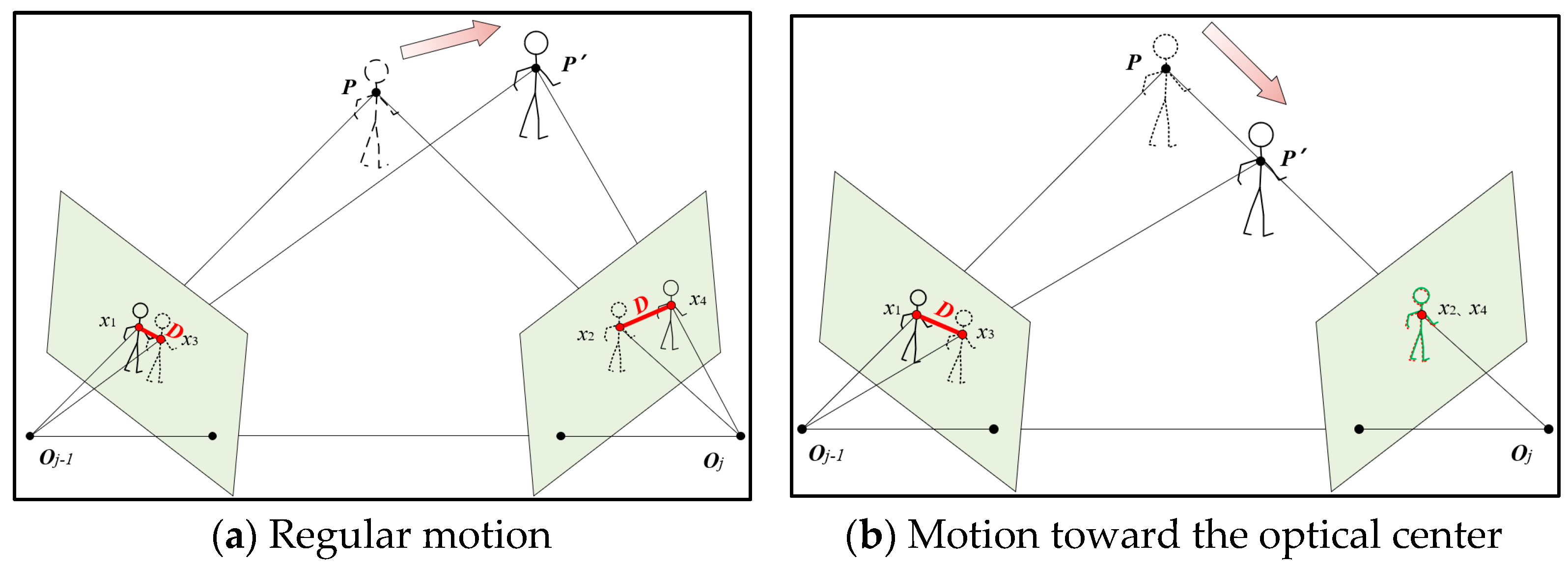
As shown in Figure 3, the red distance represents the dynamic factor of the IMU reprojection error. It shows the observation and projection of the static map point P and the dynamic point P′ in two camera frames. O denotes the camera’s optical center. and are feature points matched for the two frames with optical flow. is the feature point projected by the static point P in the th camera frame. is the feature point projected by the dynamic point P′ in the (j − 1)th camera frame.
Generally, determining the dynamics of an object through feature points’ reprojection error is effective. However, this method may fail when the dynamic object is moving along the camera’s optical center, either towards or away from the camera, as shown in Figure 3. In such cases, the reprojection error becomes close to 0, even if point P is not a dynamic point. To address this limitation, we propose an additional reprojection error on the previous frame, alongside the conventional visual reprojection in Equation (8). By incorporating both reprojection processes, the method becomes complementary, minimizing the impact on the dynamic judgment of feature points with special object motion directions. Consequently, the first part of the dynamic factors is obtained as shown below:
3.2.2. Dynamic Factor of Epipolar Constraints
An epipolar constraint is a critical property that restricts the position of feature points, commonly used in various SLAM systems to accelerate the matching process in the front end. In D-VINS, data association between feature points is achieved using the pyramidal iterative Lucas–Kanade optical flow. Subsequently, the fundamental matrix between two camera frames is computed using the seven-point method based on RANSAC.
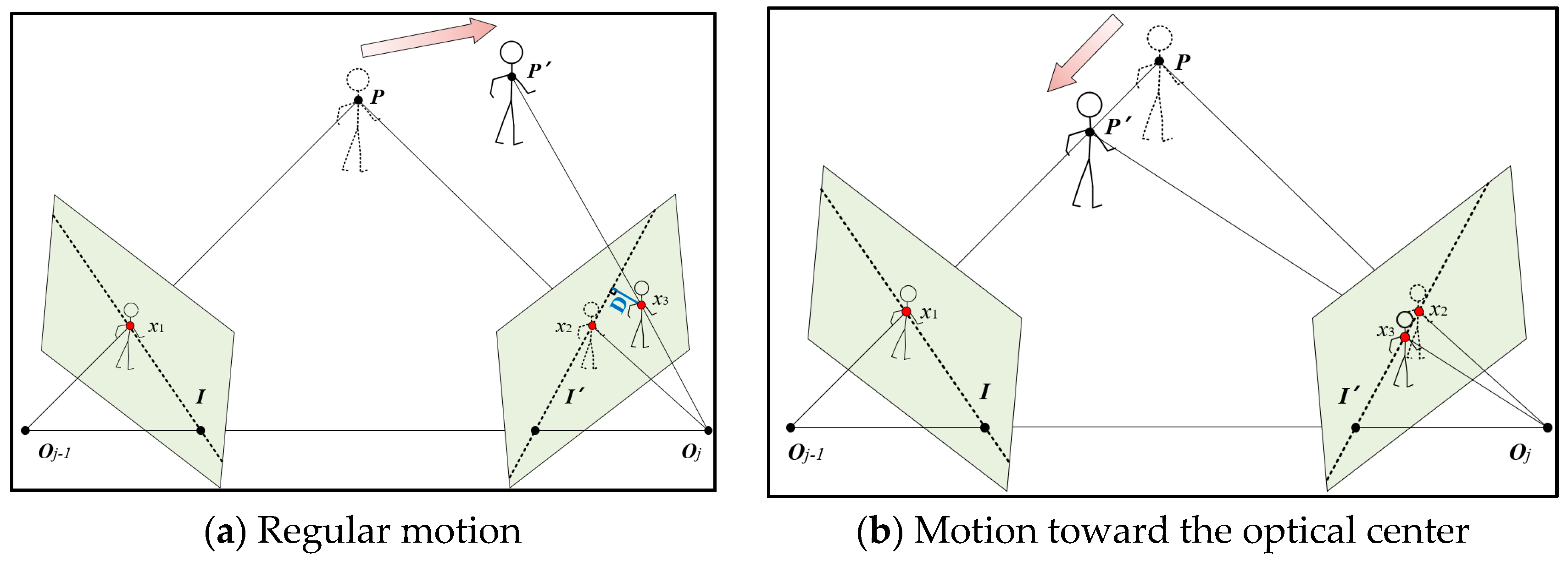
Using the fundamental matrix, the epipolar lines of feature points in the current frame are calculated. The distance from a point to its epipolar line is defined as the second part of the dynamic factor. This distance is then utilized to determine whether the point is dynamic or not. According to the pinhole camera model, the map point P is observed in different camera frames, which is shown in Figure 4. x1 and x3 are matched feature points in different frames, and x2 is the feature point projected to theth frame by the map point P. The short dashed lines I and I’ are the epipolar lines of the two frames.
are the homogeneous co-ordinate forms of the two matched feature points, belonging to the (j − 1)th frame andth frame, respectively. Then, the epipolar line of in the jth frame is as follows:
where, , anddenote the real constants in the general form of a straight line (Xu + Yv + Z = 0), and F denotes the fundamental matrix. Then, for the feature point , the epipolar constraint is as follows:
In Figure 4, the distance from the point to the epipolar line is marked by the blue line. For the matched feature point of , the residual of the epipolar constraint can be described as follows:
Then, the second part of the dynamic factor is obtained as shown below:
For the features of static objects, should be 0 or close to 0. But, for the features of dynamic objects, like P′, there is an offset between the real pixel co-ordinates and their observation. However, when the feature point moves toward the optical center of the (j − 1)th frame, the feature point is still on its epipolar line. Therefore, it is hard to determine whether the object is in motion or not. Therefore, when determining whether features are moving, the two distances of and need to be combined.
The threshold of the reprojection dynamic factor is set to 4 pixels, and the of the epipolar dynamic factor is set to 3 pixels. If the errors exceed those thresholds, then the feature points are considered absolute dynamic points and rejected. Then, the feature is marked as ADP. Thus far, the two dynamic factors and have been obtained.
This method enables a more accurate classification of temporary static objects and finds the dynamic feature points. In addition, the feature points of dynamic objects with small movements can be fully utilized by the SLAM system. The specific algorithm steps are shown in Algorithm 2.
| Algorithm 2: Dynamic feature rejection algorithm. |
| Input: Previous frame ; current frame; previous frame’s feature points ; current frame’s feature points ; the threshold of the reprojection dynamic factor; the threshold of the epipolar dynamic factor . Output: Current frame’s feature points’ dynamic factors and; current frame’s feature points’ dynamic label. |
| 1: for each in this Frame do: 2: if (.dynamics_lable == Temporary Static Point) do: 3: F_Maxtrix = cv::FindFundamentalMat(, , CV_FM_RANSAC); 4: .A = CalIMUProjectDis(,); 5: .B = CalEpipolarDis(,, F_Maxtrix); 6: if ((A >)&&(B >)) do: 7: .dynamics_lable = ADP1; 8: end if 9: end for |
3.3. Dynamic Adaptive Bundle Adjustment
The current conventional bundle adjustment optimization treats all feature points with the same weight. This study designs a novel bundle adjustment optimization algorithm based on the dynamic factor.
3.3.1. Conventional Bundle Adjustment Optimization
In the conventional visual–inertial state estimator, the bundle adjustment optimization equation is as follows:
where denotes the Huber kernel function; represents the marginalization residuals; represents the IMU pre-integration residuals; represents the visual reprojection error; represents the marginalization of the measurement state estimation matrix; represents an IMU observation; represents a visual observation; denotes the covariance of the IMU measurement; denotes the visual covariance; represents the set of all IMU observations; represents the set of tracked features in the sliding window; and denotes the estimated states to be optimized.
The traditional bundle adjustment formulation cannot reject or adjust the weights of dynamic feature points. Eliminating all temporary static points would result in insufficient visual observations for optimization, leading to unstable or erroneous BA optimization results. Thus, a more robust approach to BA optimization needs to be implemented.
3.3.2. Dynamic Adaptive Cost Function with Dynamic Factors
The novel cost function introduced in this study possesses two main features. Firstly, it facilitates the rejection of dynamic features. Secondly, it adjusts the weights of feature points during optimization based on the dynamic factors. Drawing inspiration from DynaVINS, we propose the form of the dynamic adaptive loss function as follows:
where and denote two dynamic factors of a feature point in the frame ; denotes the weights of feature points, where the weight is fixed to 1 for absolute static points; and represents the dynamic label, which will be 1 for absolute static points and 0 for temporary static points. Equation (17) presents the dynamic factors. For absolute static points, is 1, and the back-end optimization loss function is the same as the conventional one. For temporary static points, the loss function will switch to shown in Equation (16). As the loss function is designed to have a nonlinear quadratic form, the optimal weights can be derived as follows:
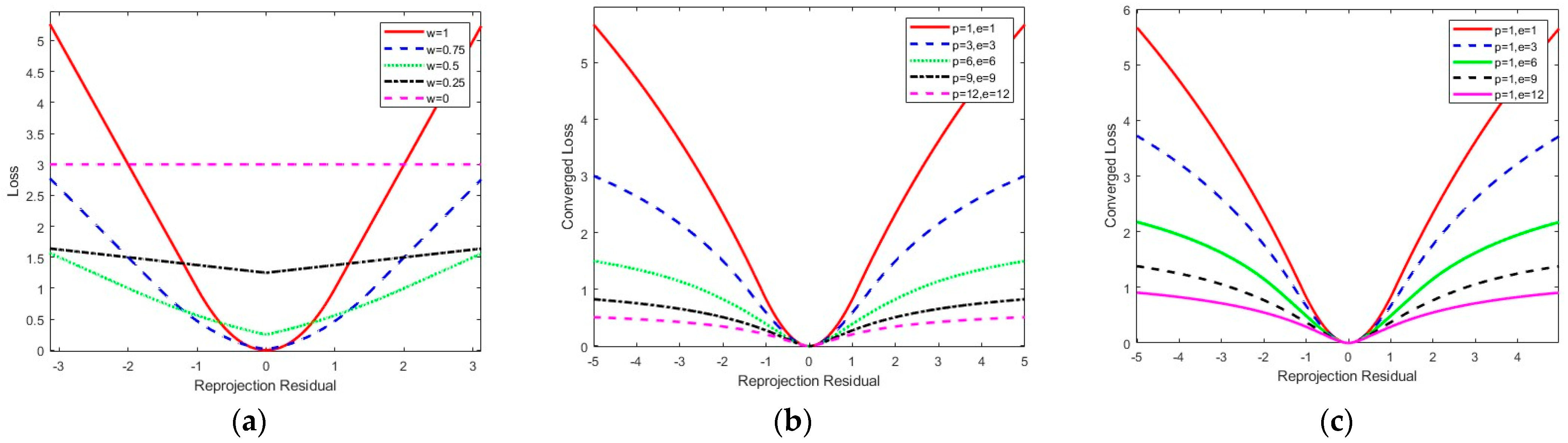
After optimizing the weights, the features with higher dynamic factors will have lower weights. The losses’ gradient of those features will be close to zero, which has no impact on BA, as shown in Figure 5a. The higher the weight assigned to feature points, the steeper the slope of the curve, indicating a greater impact on the nonlinear optimization process.
Different dynamic factors affect the gradient value and adjust the BA residuals with marginalization and IMU pre-integration residuals. Equation (16) in quadratic form is designed for nonlinear optimization. As increases, the gradient value of the converged loss function decreases, resulting in a smaller weight assigned to the corresponding features during the optimization process, as shown in Figure 5b.
When a feature point moves toward the optical center, the value of the reprojected dynamic factor is typically small. However, if the feature point exhibits a larger dynamic factor due to epipolar constraints, will be smaller, resulting in a smaller weight, as shown in Figure 5c.
Different from DynaVINS, the weight momentum factor does not need the help of semantic labels, and the point weights are delivered with bounding boxes. The total cost function based on the dynamic factors is as follows:
The strategy is to increase the weight of absolute static points and decrease the weight of temporary static points in BA optimization, completely discarding absolute dynamic points in the optimization. The weights of feature points are optimized to obtain more robust localization results. In optimizing the current state , the weights of each feature point are fixed. After that, the current state is fixed, and the feature points’ weights are optimized according to the dynamic adaptive cost function, which is as follows:
Since the feature points’ weights are independent from each other, the overall loss function is obtained by accumulating the cost equations of each feature point:
Ultimately, different optimization weights can be used based on different dynamic factors of the feature points.
4. Experimental Results
In this section, we validate the effectiveness of D-VINS by conducting experiments on publicly available datasets, including TUM RGB-D [32], KITTI [33], and VIODE [34]. These datasets offer diverse dynamic scenes for testing the algorithm’s performance.
TUM RGB-D is a widely used dynamic SLAM measurement dataset, containing monocular camera and RGBD information. VIODE is a simulation dataset specifically designed for algorithm performance testing. It is generated using a drone equipped with a stereo camera and IMU. The KITTI dataset is utilized to evaluate the algorithm’s performance in urban vehicle platforms.
In this paper, the root mean square error (RMSE) of the absolute trajectory error (ATE) [35] and the root mean square value of the relative pose error (RPE) were selected as evaluation metrics. The unit of the ATE is m. The unit of translational drift in the RPE is m/s. The ATE is well-suited to measuring the global consistency of the trajectory, while the RPE is well-suited to measuring the translation and rotation drift. They represent the global consistency of the trajectory and the drift of the odometer per unit time, respectively. Given the estimation state and the ground truth , ATE-RMSE and RPE-RMSE are calculated as follows:
where n is the number of frames in the data sequence, and ∆ is a time interval. The experimental results were analyzed both qualitatively and quantitatively. To facilitate the experiments, we integrated D-VINS with ROS, and all tests were conducted on a laptop equipped with 16 GB RAM (CPU: AMD Ryzen7 5800H, made by AMD USA, GPU: NVIDIA GEFORCE RTX 3050TI, made by NVIDIA Corporation USA). We evaluated the improvement of our proposed system, D-VINS, compared to the original algorithms ORB-SLAM2, and ORB-SLAM3. Additionally, we compared D-VINS with the state-of-the-art dynamic VSLAM algorithm, DynaVINS, as well as other similar algorithms such as DS-SLAM, RS-SLAM, and Dynamic-VINS, to further assess its effectiveness.
4.1. TUM RGB-D, VIODE, and KITTI Dataset Evaluation
4.1.1. TUM RGB-D Dataset
The TUM RGB-D dataset was captured using a Microsoft Kinect camera, made by Microsoft USA, at a frame rate of 30 Hz. It consists of 39 image sequences containing both color and depth images. This dataset has become widely used for evaluating visual odometry in dynamic scenes. The ground truth is obtained through a high-precision motion capture system. This dataset provides nine sequences for dynamic scenes, where dynamic objects can be divided into low- and high-dynamic sequences. The low-dynamic sequences are labeled “sitting” (fr3/sitting_static, fr3/sitting_xyz, fr3/sitting_halfsphere, fr3/sitting_rpy); and the high-dynamic sequences are labeled “walking” (fr3/walking_static, fr3/walking_xyz, fr3/walking_halfsphere, fr3/walking_rpy).
In this paper, we used the open-source trajectory evaluation tool Evo (available online: https://github.com/MichaelGrupp/evo (accessed on 25 April 2023)) to visualize the trajectory differences between D-VINS and ORB-SLAM2. In addition, the TUM dataset contains no IMU data, and VINS does not support monocular VO mode, so modules containing IMUs were excluded from D-VINS for the experiment. The data were obtained from the actual experiments on the dataset. There are the hyperparameters used in D-VINS, the number of feature points (150), and the pixel spacing of feature points (25); and the initial value of the dynamic factor of the feature point is .
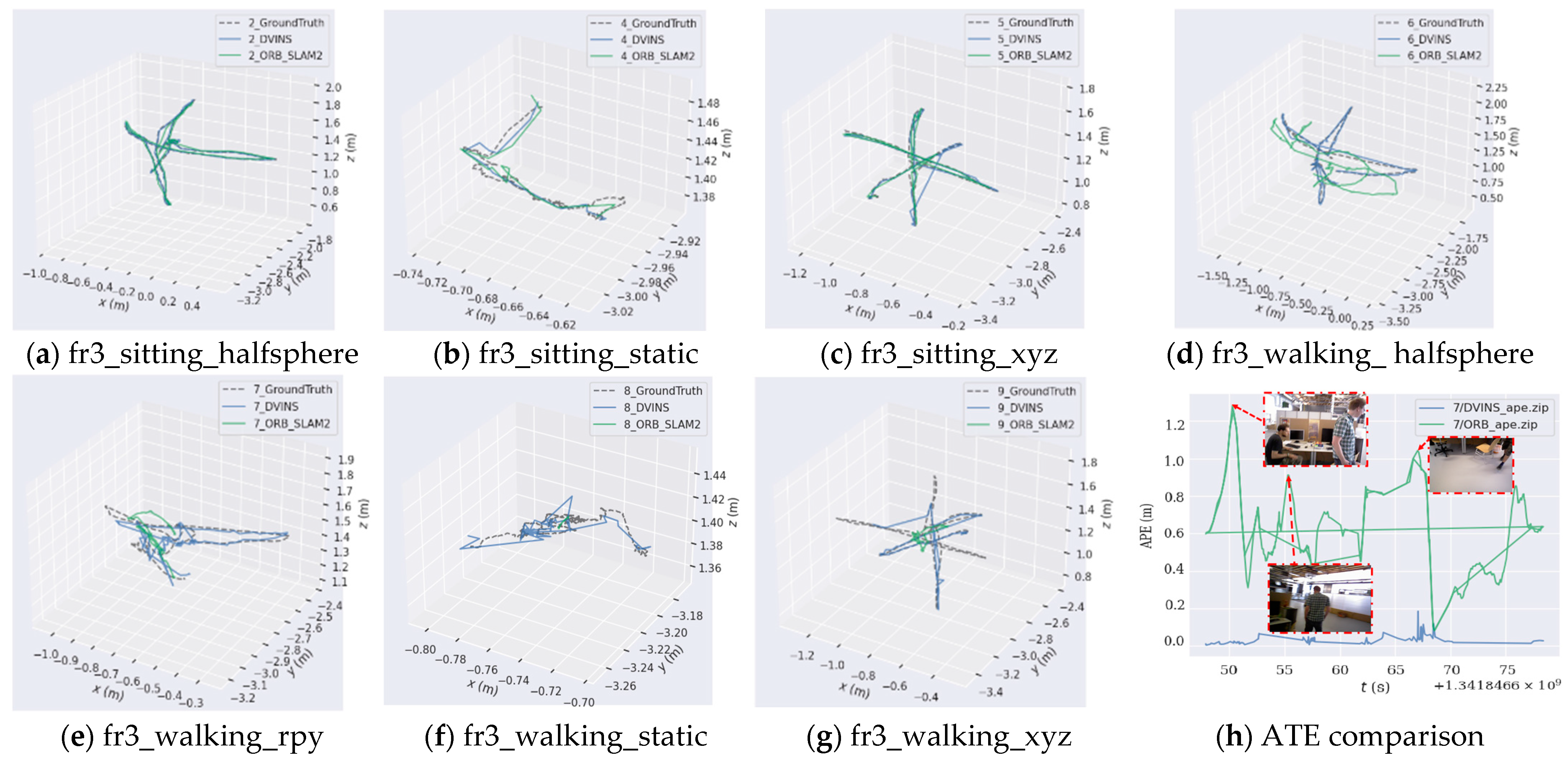
Firstly, Figure 6 shows the plotted trajectories of the two algorithms. The black dashed line represents the ground truth, provided by the dynamic capture. The blue solid line represents the trajectory generated by D-VINS, and the green solid line represents the trajectory generated by ORB-SLAM2 for comparative analysis. The quantitative analysis of this figure fully demonstrates the necessity of dynamic object rejection and the effectiveness of D-VINS. According to Figure 6h, it can be seen that, when dynamic objects appear, the trajectory accuracy is seriously impaired.
Secondly, Table 1 and Table 2 summarize the quantitative experimental results, showing a comparison with several outstanding SLAM algorithms, like ORB-SLAM3 [7], RS-SLAM [23], and Dynamic-VINS [24]. Among these contrasting SLAM methods, ORB-SLAM3 is the most accurate VSLAM open-source algorithm for evaluating the positioning accuracy of D-VINS in non-dynamic environments. RS-SLAM is a robust semantic RGB-D SLAM system that can achieve real-time high-accuracy localization based on semantic segmentation. The horizontal line in (h) represents loopback detection. Dynamic-VINS is an optimization-based RGB-D inertial odometry system providing real-time state estimation results for resource-restricted platforms.
According to Table 1, D-VINS outperformed ORB-SLAM2 in six sequences and ORB-SLAM3 in four dynamic sequences. In the sequences fr3_sitting_xyz and fr3_sitting_halfs, even though D-VINS did not achieve the highest positioning accuracy, it obtained sub-optimal accuracy in the camera absolute pose estimation. ORB-SLAM2 was unable to identify dynamic point features, and its camera pose accuracy was the weakest of all compared SLAM algorithms.
In Table 2, the compared methods’ results are presented, as reported in their original published papers. It is not difficult to find that D-VINS obtained the two best results from the four groups of experiments. In the fr3_walking_static and fr3_walking_xyz sequences, D-VINS obtained sub-optimal accuracy compared with the three other SLAM methods. The reliability of dynamic object recognition and rejection with deep learning and geometric constraints was verified with this dataset. RS-SLAM utilizes PSPNet for pixel-level segmentation and depth information, resulting in a higher accuracy in dynamic feature detection. It provides highly precise localization results when the number of dynamic feature points is limited. Dynamic-VINS just simply disables modules relevant to the IMU. Therefore, its robustness and accuracy were weaker in high-dynamic sequences. DS-SLAM exhibited severe accuracy degradation in fr3_walking_rpy. This is attributed to the non-texture and pure rotational motion, which affect the estimation of epipolar lines and camera poses. Additionally, significant occlusions occur when people pass in front of the camera, as the features’ weights are not adjusted. It should be noted that D-VINS does not incorporate pixel-level segmentation results and relies on bounding boxes, which introduces feature point segmentation errors. However, the advantage of D-VINS lies in its efficient processing speed.
4.1.2. KITTI Dataset
The KITTI dataset provides sequences containing stereo color images in the 00 to 10 urban street and highway environments for evaluating the accuracy of odometry localization. The hyperparameters used in D-VINS are: the number of feature points (150), the pixel spacing of feature points (35), the maximum number of optimizations (5), and the initial value of the dynamism factor of the feature point (). The parameters for DynaVINS in KITTI are: .
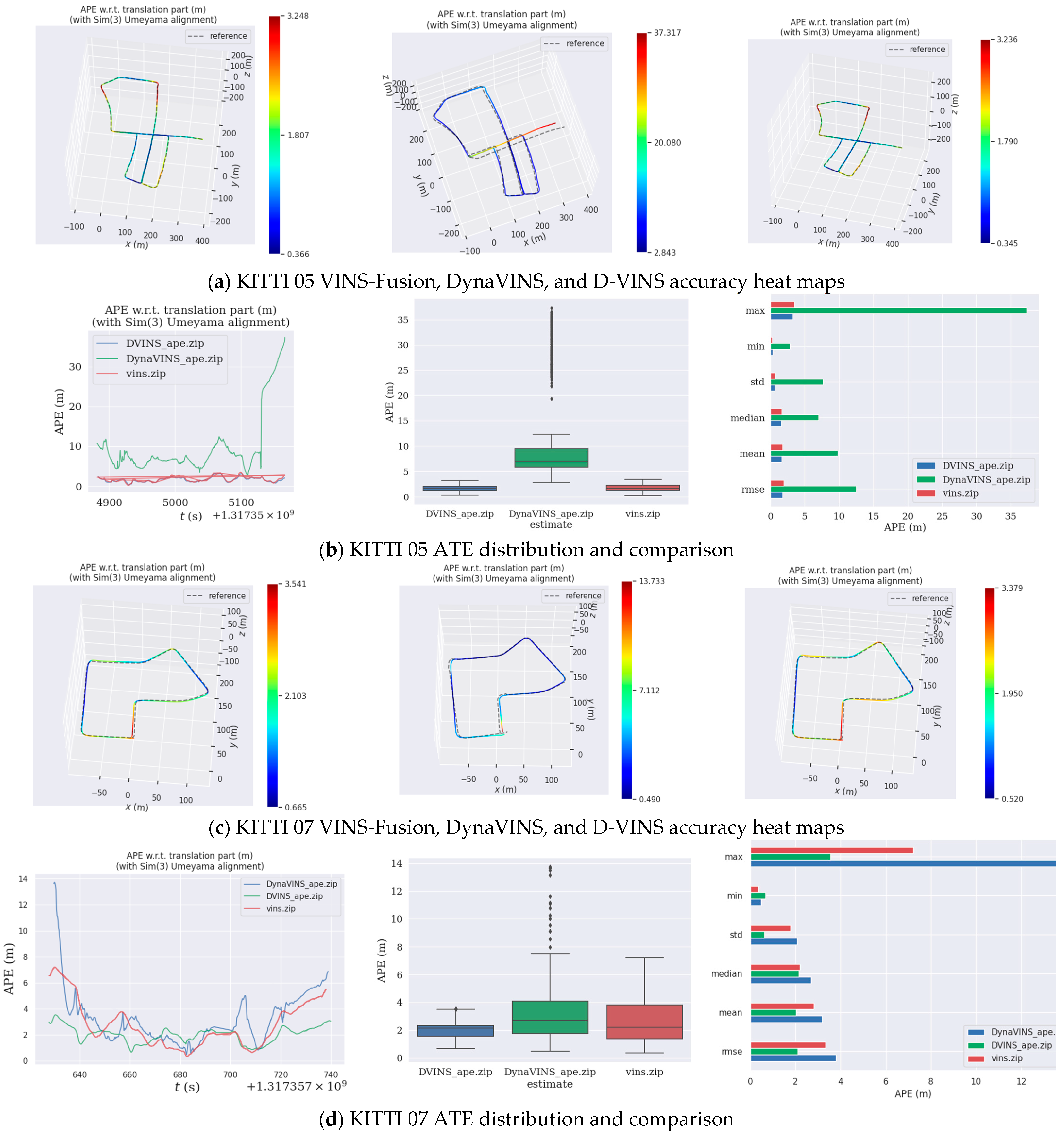
Table 3 shows the results of the 05 and 07 sequences in comparison with VINS-Fusion and DynaVINS, and the bolded data indicate the best performance, as shown in Figure 7. Since dynamic objects on both the 00 and 05 sequence streets are sparse, dynamic object rejection provides a limited improvement to the system’s accuracy. The experimental data were obtained from real measurements, rather than directly from the paper, to compare the generalizability of the algorithms. As shown in Table 3, the localization accuracy and dynamic feature recognition rejection of DynaVINS are highly dependent on the hyperparameters (momentum factor and regularization factor). Therefore, its localization results in different datasets are worse, and it is hard to keep the algorithm localized with high accuracy even after a long period of parameter adjustment. The experimental results on the KITTI dataset show that D-VINS has better generalizability than DynaVINS, as well as a certain accuracy improvement compared to VINS-Fusion.
4.1.3. VIODE Dataset
VIODE is a simulation dataset for testing VIO performance in dynamic environments such as urban areas, filling the gap in dynamic VIO system evaluation. The dataset simulates the UAV localization problem in different dynamic environments (daytime city street environment, dark city street environment, and underground parking environment). Each scene is divided into four sequences according to the number of dynamic objects: 0_none, 1_low, 2_mid, and 3_high have a total of 12 sequences. In the high sequences, the camera field of view is included with the entire occlusion to evaluate the localization accuracy and system robustness of the VIO in extreme situations. The dataset contains time-synchronized stereo color images, IMU data, an instance segmentation mask, and the ground truth of the trajectory.
To validate the accuracy of the algorithm in the dynamic recognition of absolute dynamic points and temporary static points, D-VINS and DynaVINS were compared. VINS-Fusion was also included in the comparison to prove the necessity and effectiveness of the dynamic rejection module. The hyperparameters used in D-VINS are: the number of feature points (150), the pixel spacing of feature points (35), the maximum number of optimizations (5), and the initial value of the dynamism factor of the feature point (). The hyperparameters in DynaVINS use the same values as in the paper, with regularization factor and momentum factor . Figure 8 shows the miss-detection compensation module. These features remain as labels as they are tracked by the optical flow. Figure 9 presents the epipolar constraint results; the points far from the epipolar line are labeled as dynamic points.
Overall, D-VINS demonstrates great pose estimation accuracy in static scenes when incorporating the dynamic factor, as illustrated in Table 4. It exhibits a better localization accuracy in low-dynamic scenes and comparable accuracy to DynaVINS in high-dynamic scenes, and, in some sequences, it even outperforms DynaVINS. Additionally, the spacing and quantity of feature points in the front end significantly affect the performance of D-VINS. In cases where remote features dominate the field of view or the feature spacing is too small, the accuracy of the stereo system is severely compromised. Thus, for the same set of parameters, D-VINS does not perform as well in the city sequence as it does in the parking lot environment. The localization accuracy of DynaVINS highly depends on the hyperparameters, such as the regularization factor and the momentum factor . However, these hyperparameters are manually tuned and lack generalization across different scenes. While they exhibit high localization accuracy in some scenes, they may not be suitable for other sequences. For example, the localization accuracy of DynaVINS in the City_day dataset is unstable.
In dynamic scenes with low occlusion, D-VINS incorporates a deep-learning module that detects dynamic objects and calculates dynamic factors with geometry. D-VINS achieves higher accuracy in screening dynamic feature points compared to DynaVINS, which only relies on geometric methods for dynamic object rejection, as observed in Figure 10b,d,f. Consequently, D-VINS achieves a better positioning accuracy in low and mid sequences. The green feature points represent absolute static points, the white feature points represent absolute dynamic points, and the purple feature points represent temporary dynamic points. However, in highly occluded environments where dynamic objects are near the camera, D-VINS may fail to detect the objects with the deep-learning network.
4.2. Data Collection Equipment and Real-Environment Dataset Experiments
To demonstrate that D-VINS can be applied to a real project, we built a self-made data acquisition device and created a dataset with it.
4.2.1. Data Collection Devices and Real Datasets
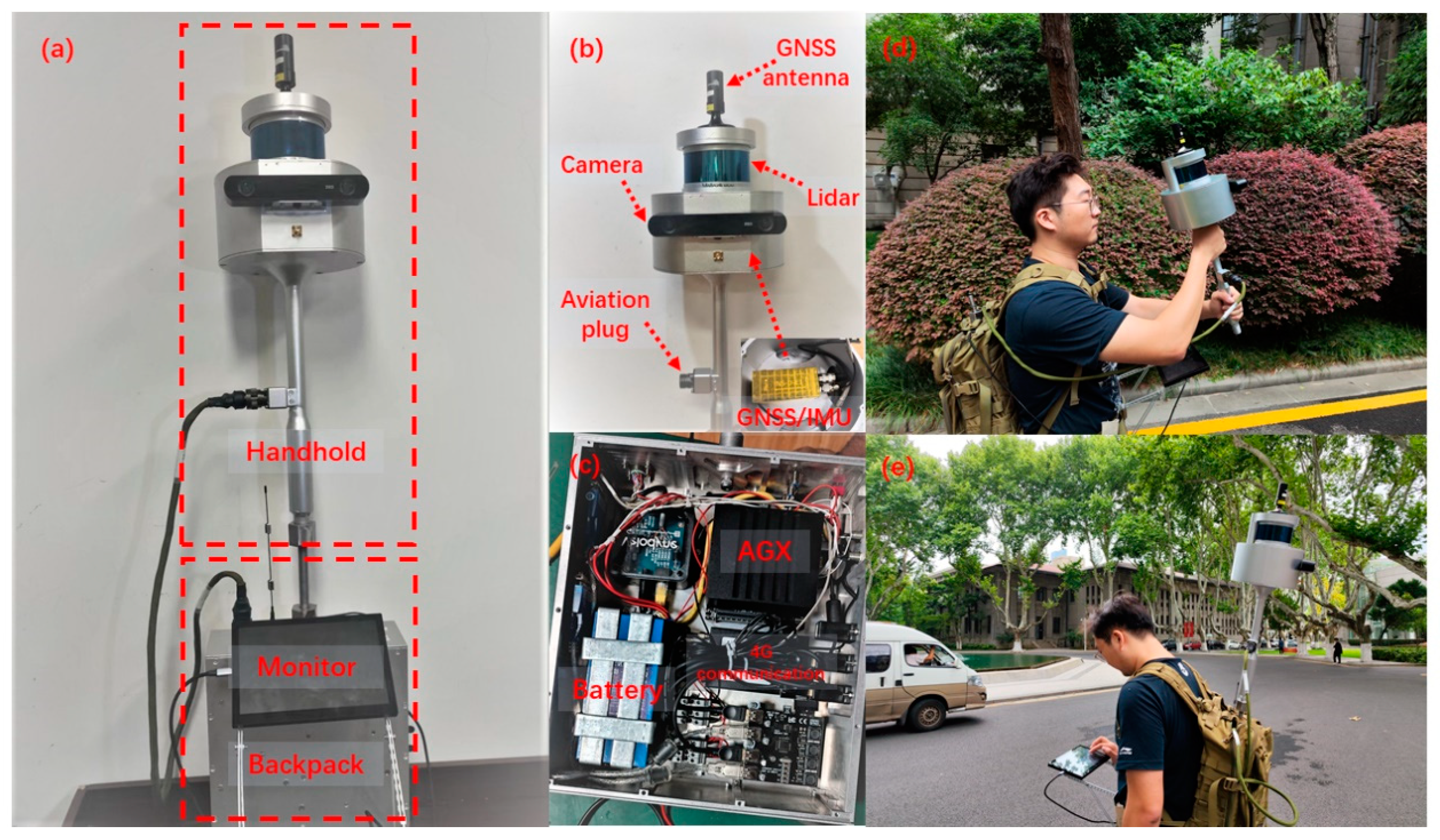
The device integrates GNSS, inertial navigation, LIDAR, and a stereo camera, and is mainly divided into two parts: the handheld part, and the backpack part. As shown in Figure 11, the device has three working modes: handheld, backpack, and vehicle working mode. The handheld part includes a GNSS antenna, Velodyne VLP-32C mechanical LIDAR, Inertial Labs INS-D GNSS/IMU inertial guidance, and a ZED2 color stereo camera, and the resolution is 1280 × 720; the backpack part includes an NVIDIA Jetson AGX Xavier processor, a 12 V DC lithium battery, an MD-649 4G DTU 4G communication module, and an antenna. In this paper, one handheld rural sequence and two city street sequences were selected for experimental validation:
- The 5_SLAM_country_dynamic_loop_1 sequence was collected in a village in Xiangyin County, Yueyang City, Hunan Province, in a relatively open environment, where a pedestrian and child were always present in the image moving in synchronization with the camera. The start and end points of the sequence are close to each other, but there is no loop to detect the drift.
- The 14_SLAM_car_road_1 sequence shows a street in Xiangyin County, Yueyang City, Hunan Province. The sequence is an open environment. This environment is challenging for stereo-visual localization, which causes severe drift. The rural roads are narrow with many vehicles, and there are villagers gathering in the middle of the road. Pedestrians and vehicles are intricate and occupy a large field of view, making positioning difficult and challenging.
- The 18_SLAM_car_road_2 sequence is an urban environment with wider roads, more vehicles, and more pedestrians compared to the 14 rural streets. It is suitable as a dynamic rejection algorithm evaluation sequence. The main data types include GNSS raw data, IMU data, LiDAR point cloud data, and binocular color image data. The ground truth of the trajectory is obtained with GNSS RTK.
4.2.2. Feature Classification Results on the Real Dataset
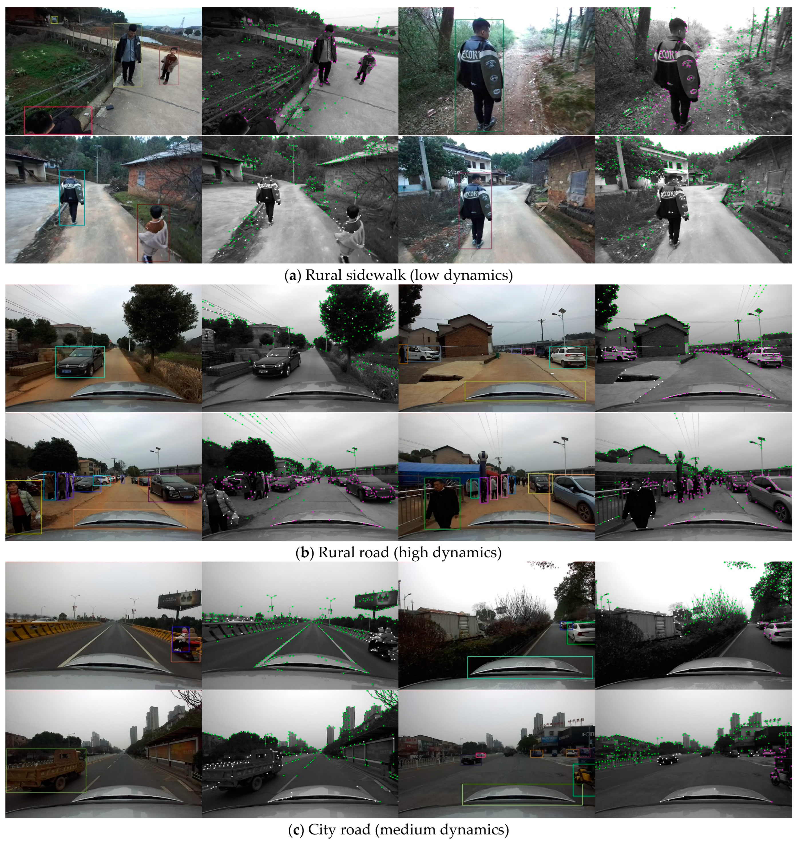
In the 5_SLAM_country_dynamic_loop_1 sequence, there are two people walking in front of the camera; this represents an easy object detection task for deep learning to accomplish. As shown in Figure 12, when the person with the jacket is moving in the second row in (a), the dynamic features are segmented accurately. When the person is movable but remains static at the current time shown in the first row in (a), those feature points are kept for optimization. In a highly dynamic sequence, the majority of the points are movable and only a few of them are moving. D-VINS is able to reject dynamic features that are close to the camera with higher dynamic factors. In the city street, the cars parked on the roadside and driving on the road are detected with different motion state classifications.
4.2.3. Trajectory Results on the Real Dataset
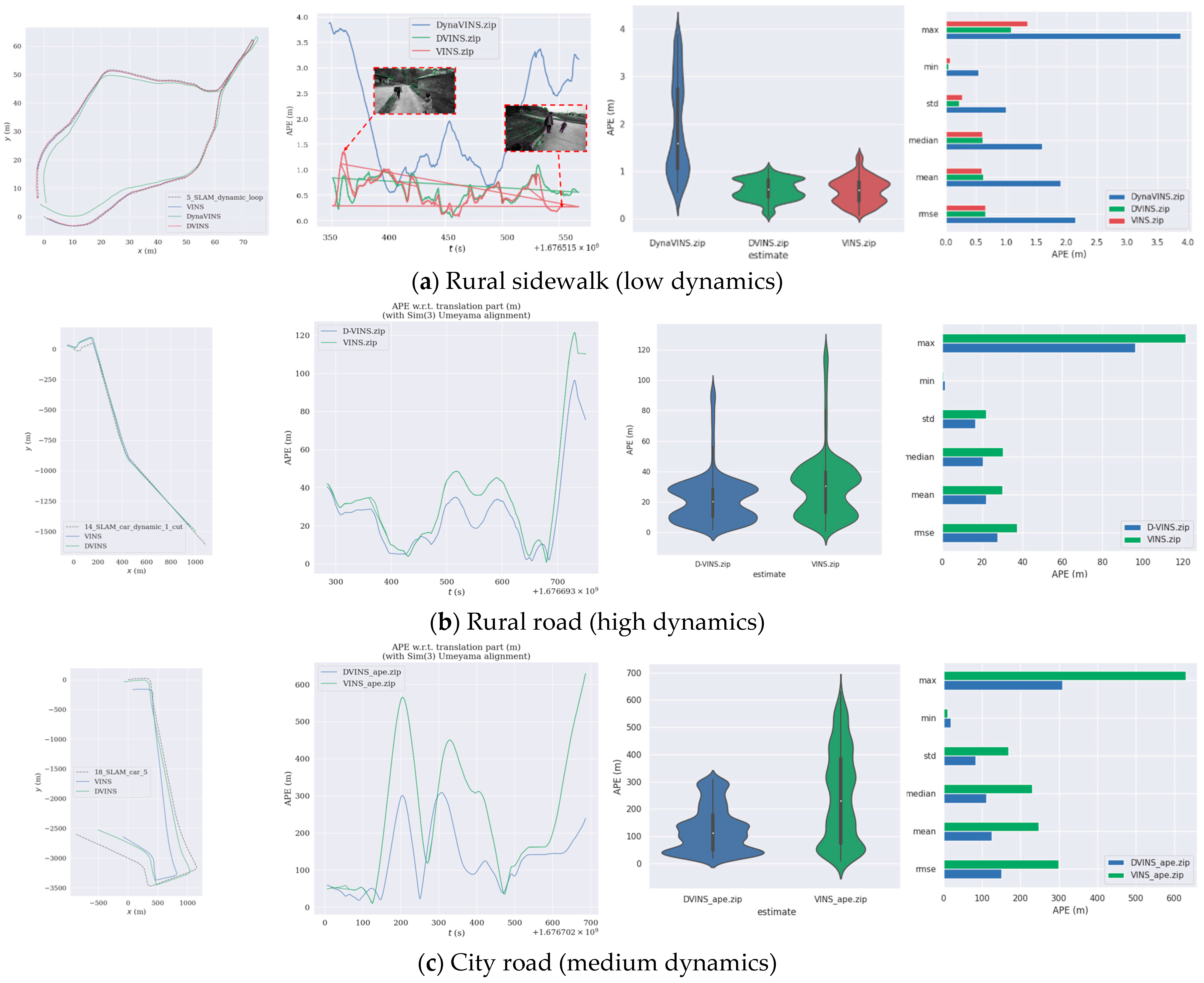
This paper compared the results of the current state-of-the-art algorithms DynaVINS, D-VINS, and VINS on real dataset sequences. D-VINS obtained better measurement results on the real dataset, effectively overcoming the influence of dynamic objects. As shown in Table 5, D-VINS obtained a better localization accuracy than DynaVINS in the 5_SLAM_dynamic_loop_1 sequence. Even though the ATE-RMSE of D-VINS was similar to that of VINS, the more detailed results show that D-VINS had a more accurate localization accuracy in the presence of dynamic objects, as well as a lower median and mean. Even after parameter adjustments, DynaVINS had difficulty finding parameters that could achieve good accuracy in localization (the hyperparameters provided in the paper could not accomplish localization, even though they worked well on the VIODE and KITTI datasets). The high reliance on equipment and hyperparameters is also a drawback for geometry-based methods. D-VINS is merely a visual odometry system, and, in the absence of GNSS and loop detection, the drift is significant. In Figure 13, D-VINS achieves excellent positioning results in two road sequences without loop detection. The pure VIO system (no global optimization and loopback detection) can effectively reduce the influence of dynamic objects and substantially exceed the positioning accuracy of VINS. In summary, D-VINS has stronger robustness and scene applicability in dynamic scenes compared to other algorithms.
4.2.4. Time Analysis and Ablation Experiment
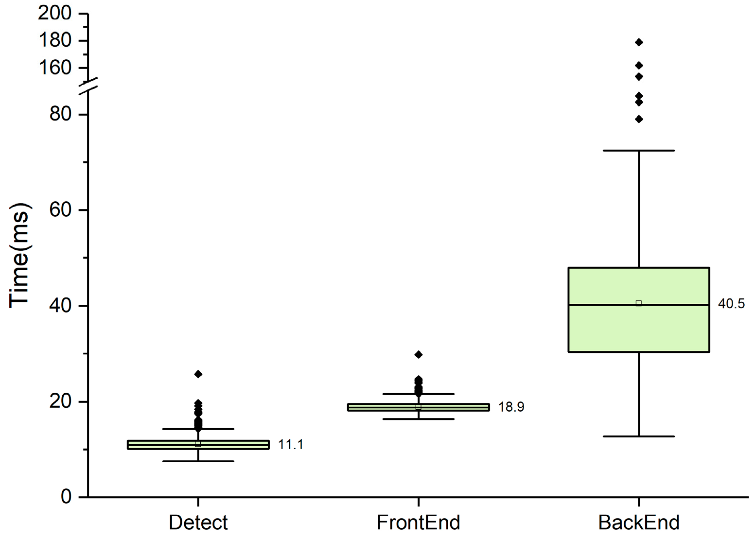
As a fundamental component of robot state estimation, SLAM plays a crucial role in the smooth execution of higher-level tasks. Therefore, we conducted tests on the average time cost of processing each frame of various frameworks. The experimental results are presented in Figure 14. All tests were conducted on a laptop equipped with 16 GB RAM (CPU: AMD Ryzen7 5800H, GPU: NVIDIA GEFORCE RTX 3050TI). Due to the inconsistent number of iterations during optimization, the overall time for back-end optimization exhibits significant variance. However, the system can operate in real time with a 10 Hz camera.
D-VINS adopts a combined approach of geometric and semantic information to remove dynamic feature points and improve accuracy, effectively incorporating the strengths of both methods while avoiding their limitations. To validate the effectiveness of the fused algorithm integrating geometric and semantic information, we conducted comparative experiments. D-VINS (G) represents a geometry-based method adjusting feature weights with epipolar constraints and IMU reprojection. D-VINS (S) represents a semantic-based method with YOLOV5. D-VINS (G + S) represents a fusion algorithm based on geometric and semantic information. The experimental results are shown in Table 6.
5. Discussion
In the experimental results shown in Table 1, Table 2, Table 3, Table 4 and Table 5, D-VINS and the contrasting SLAM systems were all validated. D-VINS outperformed the other systems in terms of the ATE and RPE in six sequences of the TUM RGB-D dataset. Table 1 and Table 2 demonstrate the effectiveness of D-VINS’ dynamic object removal method, especially in scenarios involving pure rotation and high-occlusion areas, compared to semantic-based methods like RS-SLAM and DS-SLAM. Moreover, RS-SLAM and Dynamic-VINS are limited to indoor usage due to their reliance on depth information, making them unsuitable for outdoor environments.
In the KITTI sequences shown in Table 3, D-VINS demonstrated its effectiveness in outdoor scenes. The state-of-the-art DynaVINS showed high accuracy in the VIODE simulation dataset, as shown in Table 4, but it heavily relied on two hyperparameters, making it challenging to achieve the same high accuracy in different datasets. In the KITTI 05 and 07 sequences, where there were fewer dynamic objects than in VIODE, the impact on position estimation was less significant, resulting in DynaVINS not performing as well as it did in VIODE, as displayed in Figure 7. For the highly occluded scenes in VIODE, deep learning struggled, especially when the objects moved toward the camera’s optical center (shown in the first image of Figure 10b). In contrast, D-VINS demonstrated good dynamic feature segmentation performance and trajectory accuracy, exhibiting better robustness in multiple environments in Figure 10b,d,f. However, the accuracy of DynaVINS decreased in sequences with fewer dynamic objects, such as the 0_none sequences. D-VINS maintains accuracy in highly occluded dynamic environments. However, its improvement in low-occlusion dynamic environments is not significant with abundant features that can be tracked.
Furthermore, D-VINS showed great performance in feature classification and trajectory accuracy in rural and city sequences, as shown in Figure 12. For our real dataset, DynaVINS faced challenges in accomplishing the localization task. Higher reprojection errors could arise from both the camera movement and dynamic features, making it difficult to accurately indicate the feature’s motion state using weights. In sequences with large spaces and without loop closures, VINS-Fusion performed worse compared to D-VINS. However, the segmentation accuracy depends on the bounding boxes obtained from YOLOV5, making it unable to achieve pixel-level precise segmentation. Factors such as the complexity of moving objects and blurry images can influence the results of object detection and geometric calculations. These influences can degrade the segmentation accuracy and, ultimately, impact the camera localization precision.
In summary, while D-VINS may not overcome extreme conditions of complete occlusion in the field of view, it still achieves a high localization accuracy in highly occluded environments, comparable to DynaVINS. D-VINS is more suitable for indoor environments with occlusions and outdoor environments with at a small scale. In large outdoor scenes, it experiences considerable drift without GNSS and loop detection. In cases where the camera’s field of view is completely occluded, the system relies more on IMU pre-integration results. The few static feature points are given higher weights in the iterative optimization process, due to dynamic factors based on epipolar constraints and IMU reprojection errors, ultimately enhancing the accuracy of the pose optimization. Extensive experimental results have proven that D-VINS can improve the accuracy and robustness of pose calculation in dynamic scenes.
6. Conclusions
In this paper, we proposed a novel dynamic VIO system designed for outdoor dynamic scenes, effectively reducing the impact of dynamic objects. The D-VINS system consists of four modules: target identification and data pre-processing, feature point classification and tracking, and back-end dynamic factor BA optimization. The dynamic object recognition relies on YOLOV5 to obtain semantic information about the scene, such as walking people and stopped cars. The semantic labels are continuously updated, classifying dynamic points into absolute dynamic points, absolute static points, and temporary static points. The dynamic factors of temporary static points are calculated using IMU pre-integration and epipolar constraints. Only absolute static points and temporary static points are sent for nonlinear optimization. Feature point weights are adjusted based on the dynamic label and dynamic factors during BA optimization. The system’s effectiveness in dynamic environments was verified using the TUM RGB-D, KITTI, and VIODE datasets, as well as our own dataset. The experimental results demonstrated our system’s superior performance compared to RS-SLAM, Dynamic-VINS, and the state-of-the-art method DynaVINS. In general, D-VINS enhances feature point weights, enabling its use in environments with occluding dynamic objects. However, the accuracy is limited by the number of optimization iterations, as excessive iterations can hinder real-time system operation. Time analysis shows that sacrificing some optimization iterations still allows for achieving a satisfactory localization accuracy while maintaining real-time performance.
Future work should address some limitations and explore potential improvements. Firstly, the algorithm lacks pixel-level segmentation of feature points, even with geometry constraints. Integrating a high-speed semantic segmentation module could help to achieve a more accurate identification of dynamic feature points in the front end. Secondly, during the experimental process, degraded scenes had an impact on the estimation. For instance, the localization accuracy of stereo cameras decreases in open environments. Adjusting the weights of feature points at different distances can improve the localization accuracy. The algorithm also exhibits good scalability, as the strategy of adjusting feature point weights can be incorporated into existing multi-sensor fusion systems. Additionally, to address occlusion issues in dynamic scenes, the target velocity can be used to introduce extra constraints on self-motion estimation.
Author Contributions
Y.S. conceived the idea and methods; data curation, Y.S., R.T. and C.Y.; software, Y.S.; Y.S. and X.S. performed the experiments and validation; C.Y. and R.T. analyzed the data; supervision, Q.W. and Y.F.; Y.S., C.Y. and R.T. wrote and revised the paper; visualization, X.W. All authors have read and agreed to the published version of the manuscript.
Funding
This research was funded by the National Natural Science Foundation of China (No.42074039). The authors would like to thank the referees for their constructive comments.
Data Availability Statement
Publicly available datasets were analyzed in this study. These data can be found here: http://vision.in.tum.de/data/datasets/rgbd-dataset, https://github.com/kminoda/VIODE, https://www.cvlibs.net/datasets/kitti/ (all accessed on 1 May 2023).
Acknowledgments
We thank the researchers who developed the TUM RGB-D, KITTI, and VIODE datasets.
Conflicts of Interest
The authors declare no conflict of interest.
References
- Kazerouni, I.A.; Fitzgerald, L.; Dooly, G.; Toal, D. A survey of state-of-the-art on visual SLAM. Expert Syst. Appl. 2022, 205, 117734. [Google Scholar] [CrossRef]
- Covolan, J.P.M.; Sementille, A.C.; Sanches, S.R.R. A Mapping of Visual SLAM Algorithms and Their Applications in Augmented Reality. In Proceedings of the 2020 22nd Symposium on Virtual and Augmented Reality (SVR), Porto de Galinhas, Brazil, 7–10 November 2020; pp. 20–29. [Google Scholar]
- Tourani, A.; Bavle, H.; Sanchez-Lopez, J.L.; Voos, H. Visual SLAM: What Are the Current Trends and What to Expect? Sensors 2022, 22, 9297. [Google Scholar] [CrossRef] [PubMed]
- Chen, C.; Zhu, H.; Li, M.; You, S. A Review of Visual-Inertial Simultaneous Localization and Mapping from Filtering-Based and Optimization-Based Perspectives. Robotics 2018, 7, 45. [Google Scholar] [CrossRef] [Green Version]
- Cvisic, I.; Markovic, I.; Petrovic, I. SOFT2: Stereo Visual Odometry for Road Vehicles Based on a Point-to-Epipolar-Line Metric. IEEE Trans. Robot. 2022, 39, 273–288. [Google Scholar] [CrossRef]
- Qin, T.; Li, P.; Shen, S. VINS-Mono: A Robust and Versatile Monocular Visual-Inertial State Estimator. IEEE Trans. Robot. 2018, 34, 1004–1020. [Google Scholar] [CrossRef] [Green Version]
- Campos, C.; Elvira, R.; Rodriguez, J.J.G.; Montiel, J.M.M.; Tardos, J.D. ORB-SLAM3: An Accurate Open-Source Library for Visual, Visual–Inertial, and Multimap SLAM. IEEE Trans. Robot. 2021, 37, 1874–1890. [Google Scholar] [CrossRef]
- von Stumberg, L.; Cremers, D. DM-VIO: Delayed Marginalization Visual-Inertial Odometry. IEEE Robot. Autom. Lett. 2022, 7, 1408–1415. [Google Scholar] [CrossRef]
- Qin, T.; Cao, S.; Pan, J.; Shen, S. A General Optimization-Based Framework for Global Pose Estimation with Multiple Sensors. arXiv 2019, arXiv:1901.03642. [Google Scholar]
- Mur-Artal, R.; Tardos, J.D. ORB-SLAM2: An Open-Source SLAM System for Monocular, Stereo, and RGB-D Cameras. IEEE Trans. Robot. 2017, 33, 1255–1262. [Google Scholar] [CrossRef] [Green Version]
- Fischler, M.A.; Bolles, R.C. Random Sample Consensus: A Paradigm for Model Fitting with Applications to Image Analysis and Automated Cartography. In Readings in Computer Vision; Fischler, M.A., Firschein, O., Eds.; Morgan Kaufmann: San Francisco CA, USA, 1987; pp. 726–740. ISBN 978-0-08-051581-6. [Google Scholar]
- Jocher, G.; Chaurasia, A.; Stoken, A.; Borovec, J.; Kwon, Y.; Michael, K.; TaoXie; Fang, J.; NanoCode012; Imyhxy; et al. Ultralytics/Yolov5: V7.0 - YOLOv5 SOTA Realtime Instance Segmentation 2022. Available online: https://zenodo.org/record/7347926 (accessed on 1 May 2023). [CrossRef]
- Yan, L.; Hu, X.; Zhao, L.; Chen, Y.; Wei, P.; Xie, H. DGS-SLAM: A Fast and Robust RGBD SLAM in Dynamic Environments Combined by Geometric and Semantic Information. Remote Sens. 2022, 14, 795. [Google Scholar] [CrossRef]
- Song, S.; Lim, H.; Lee, A.J.; Myung, H. DynaVINS: A Visual-Inertial SLAM for Dynamic Environments. IEEE Robot. Autom. Lett. 2022, 7, 11523–11530. [Google Scholar] [CrossRef]
- Zhang, C.; Zhang, R.; Jin, S.; Yi, X. PFD-SLAM: A New RGB-D SLAM for Dynamic Indoor Environments Based on Non-Prior Semantic Segmentation. Remote Sens. 2022, 14, 2445. [Google Scholar] [CrossRef]
- Bian, J.; Lin, W.-Y.; Matsushita, Y.; Yeung, S.-K.; Nguyen, T.-D.; Cheng, M.-M. GMS: Grid-Based Motion Statistics for Fast, Ultra-Robust Feature Correspondence. In Proceedings of the 2017 IEEE Conference on Computer Vision and Pattern Recognition (CVPR), Honolulu, HI, USA, 21–26 July 2017; pp. 2828–2837. [Google Scholar]
- Huang, J.; Yang, S.; Zhao, Z.; Lai, Y.-K.; Hu, S. ClusterSLAM: A SLAM Backend for Simultaneous Rigid Body Clustering and Motion Estimation. In Proceedings of the 2019 IEEE/CVF International Conference on Computer Vision (ICCV), Seoul, Repiblic of Korea, 27 October–2 November 2019; pp. 5874–5883. [Google Scholar]
- Bescos, B.; Facil, J.M.; Civera, J.; Neira, J. DynaSLAM: Tracking, Mapping, and Inpainting in Dynamic Scenes. IEEE Robot. Autom. Lett. 2018, 3, 4076–4083. [Google Scholar] [CrossRef] [Green Version]
- Xiao, L.; Wang, J.; Qiu, X.; Rong, Z.; Zou, X. Dynamic-SLAM: Semantic monocular visual localization and mapping based on deep learning in dynamic environment. Robot. Auton. Syst. 2019, 117, 1–16. [Google Scholar] [CrossRef]
- Liu, W.; Anguelov, D.; Erhan, D.; Szegedy, C.; Reed, S.; Fu, C.-Y.; Berg, A.C. SSD: Single Shot MultiBox Detector. In Proceedings of the Computer Vision—ECCV 2016, Amsterdam, The Netherlands, 11–14 October 2016; Leibe, B., Matas, J., Sebe, N., Welling, M., Eds.; Springer International Publishing: Cham, Switzerland, 2016; pp. 21–37. [Google Scholar]
- Yu, C.; Liu, Z.; Liu, X.-J.; Xie, F.; Yang, Y.; Wei, Q.; Fei, Q. DS-SLAM: A Semantic Visual SLAM towards Dynamic Environments. In Proceedings of the 2018 IEEE/RSJ International Conference on Intelligent Robots and Systems (IROS), Madrid, Spain, 1–5 October 2018; pp. 1168–1174. [Google Scholar] [CrossRef] [Green Version]
- Lucas, B.D.; Kanade, T. An Iterative Image Registration Technique with an Application to Stereo Vision. In Proceedings of the DARPA Image Understanding Workshop, Washington, DC, USA, 21–23 April 1981; pp. 674–679. [Google Scholar]
- Ran, T.; Yuan, L.; Zhang, J.; Tang, D.; He, L. RS-SLAM: A Robust Semantic SLAM in Dynamic Environments Based on RGB-D Sensor. IEEE Sens. J. 2021, 21, 20657–20664. [Google Scholar] [CrossRef]
- Liu, J.; Li, X.; Liu, Y.; Chen, H. Dynamic-VINS: RGB-D Inertial Odometry for a Resource-Restricted Robot in Dynamic Environments. IEEE Robot. Autom. Lett. 2022, 7, 9573–9580. [Google Scholar] [CrossRef]
- Wu, W.; Guo, L.; Gao, H.; You, Z.; Liu, Y.; Chen, Z. YOLO-SLAM: A semantic SLAM system towards dynamic environment with geometric constraint. Neural Comput. Appl. 2022, 34, 6011–6026. [Google Scholar] [CrossRef]
- Cheng, S.; Sun, C.; Zhang, S.; Zhang, D. SG-SLAM: A Real-Time RGB-D Visual SLAM Toward Dynamic Scenes With Semantic and Geometric Information. IEEE Trans. Instrum. Meas. 2023, 72, 7501012. [Google Scholar] [CrossRef]
- Lin, T.-Y.; Maire, M.; Belongie, S.; Hays, J.; Perona, P.; Ramanan, D.; Dollár, P.; Zitnick, C.L. Microsoft COCO: Common Objects in Context. In Proceedings of the Computer Vision—ECCV 2014, Zurich, Switzerland, 6–12 September 2014; Fleet, D., Pajdla, T., Schiele, B., Tuytelaars, T., Eds.; Springer International Publishing: Cham, Switzerland, 2014; pp. 740–755. [Google Scholar]
- Shi, J. Tomasi Good Features to Track. In Proceedings of the IEEE Conference on Computer Vision and Pattern Recognition CVPR-94, Seattle, WA, USA, 21–23 June 1994; IEEE Comput. Soc. Press: Seattle, WA, USA, 1994; pp. 593–600. [Google Scholar]
- Shafi, O.; Rai, C.; Sen, R.; Ananthanarayanan, G. Demystifying TensorRT: Characterizing Neural Network Inference Engine on Nvidia Edge Devices. In Proceedings of the 2021 IEEE International Symposium on Workload Characterization (IISWC), Storrs, CT, USA, 7–9 November 2021; pp. 226–237. [Google Scholar]
- Wang, Q.; Yan, C.; Tan, R.; Feng, Y.; Sun, Y.; Liu, Y. 3D-CALI: Automatic Calibration for Camera and LiDAR Using 3D Checkerboard. Measurement 2022, 203, 111971. [Google Scholar] [CrossRef]
- Rehder, J.; Nikolic, J.; Schneider, T.; Hinzmann, T.; Siegwart, R. Extending Kalibr: Calibrating the Extrinsics of Multiple IMUs and of Individual Axes. In Proceedings of the 2016 IEEE International Conference on Robotics and Automation (ICRA), Stockholm, Sweden, 16–21 May 2016; pp. 4304–4311. [Google Scholar]
- Sturm, J.; Engelhard, N.; Endres, F.; Burgard, W.; Cremers, D. A Benchmark for the Evaluation of RGB-D SLAM Systems. In Proceedings of the 2012 IEEE/RSJ International Conference on Intelligent Robots and Systems, Vilamoura-Algarve, Portugal, 7–12 October 2012; pp. 573–580. [Google Scholar]
- Geiger, A.; Lenz, P.; Stiller, C.; Urtasun, R. Vision meets robotics: The KITTI dataset. Int. J. Robot. Res. 2013, 32, 1231–1237. [Google Scholar] [CrossRef] [Green Version]
- Minoda, K.; Schilling, F.; Wuest, V.; Floreano, D.; Yairi, T. VIODE: A Simulated Dataset to Address the Challenges of Visual-Inertial Odometry in Dynamic Environments. IEEE Robot. Autom. Lett. 2021, 6, 1343–1350. [Google Scholar] [CrossRef]
- Zhang, Z.; Scaramuzza, D. A Tutorial on Quantitative Trajectory Evaluation for Visual(-Inertial) Odometry. In Proceedings of the 2018 IEEE/RSJ International Conference on Intelligent Robots and Systems (IROS), Madrid, Spain, 1–5 October 2018; pp. 7244–7251. [Google Scholar]
Figure 1.
Overview of D-VINS. Absolute dynamic points are eliminated (indicated by the red dashed line). Temporary static points and absolute static features are shown by the blue and green arrows, respectively. The feature dynamic check module further filters out some absolute dynamic points, ensuring that only absolute static feature points are sent to the keyframe database.

Figure 2.
Dynamic object hierarchy. The common objects in the COCO dataset are classified based on life experience. Objects are categorized into different levels based on their potential motion. Levels I and II correspond to static objects, Levels III and IV correspond to temporary static objects, and Level V corresponds to dynamic objects.

Figure 3.
Reprojection error based on IMU prior constraint for temporary static points. (a) Reprojection process with IMU pre-integration. (b) A special case for moving toward the optical center Oj. The red line represents the reprojection error. The short dashed line indicates that the object is static. For the convenience of viewing, the green and red lines represent the overlapping parts, in (b).

Figure 4.
Epipolar constraint for temporary static points. (a) Epipolar constraint in regular cases. (b) A special case for moving toward the optical center . The blue line represents the distance between the feature point and its epipolar line. The short dashed lines indicate the epipolar lines.
Figure 4.
Epipolar constraint for temporary static points. (a) Epipolar constraint in regular cases. (b) A special case for moving toward the optical center . The blue line represents the distance between the feature point and its epipolar line. The short dashed lines indicate the epipolar lines.

Figure 5.
Changes in loss with various parameters. (a) Loss of one feature with . (b) Converged loss of one feature with different dynamic factors, and . (c) Converged loss of one feature with fixed.
Figure 5.
Changes in loss with various parameters. (a) Loss of one feature with . (b) Converged loss of one feature with different dynamic factors, and . (c) Converged loss of one feature with fixed.

Figure 6.
Comparison of trajectory results of D-VINS (blue) and ORB-SLAM2 (green) on the TUM datasets. (a–g) are the trajectory comparison results for each sequence of the TUM RGB-D dataset. (h) is the comparison results of the two algorithms for the fr3_walking_rpy sequence. The horizontal axis represents time in seconds, and the longitudinal axis represents the ATE in meters.

Figure 7.
Comparison trajectory results of VINS-Fusion, DynaVINS, and D-VINS on the KITTI 05 and 07 sequences. (a,b) present the accuracy heat maps and comparison results for the 05 sequence, and (c,d) present those for the 07 sequence, respectively.
Figure 7.
Comparison trajectory results of VINS-Fusion, DynaVINS, and D-VINS on the KITTI 05 and 07 sequences. (a,b) present the accuracy heat maps and comparison results for the 05 sequence, and (c,d) present those for the 07 sequence, respectively.

Figure 8.
Result of the YOLOV5 detection test. Top: original detection results of YOLOV5. Bottom: detection results after using the compensation algorithm in Section 3.1.1. The red box shows the position of clustered features for compensation.
Figure 8.
Result of the YOLOV5 detection test. Top: original detection results of YOLOV5. Bottom: detection results after using the compensation algorithm in Section 3.1.1. The red box shows the position of clustered features for compensation.

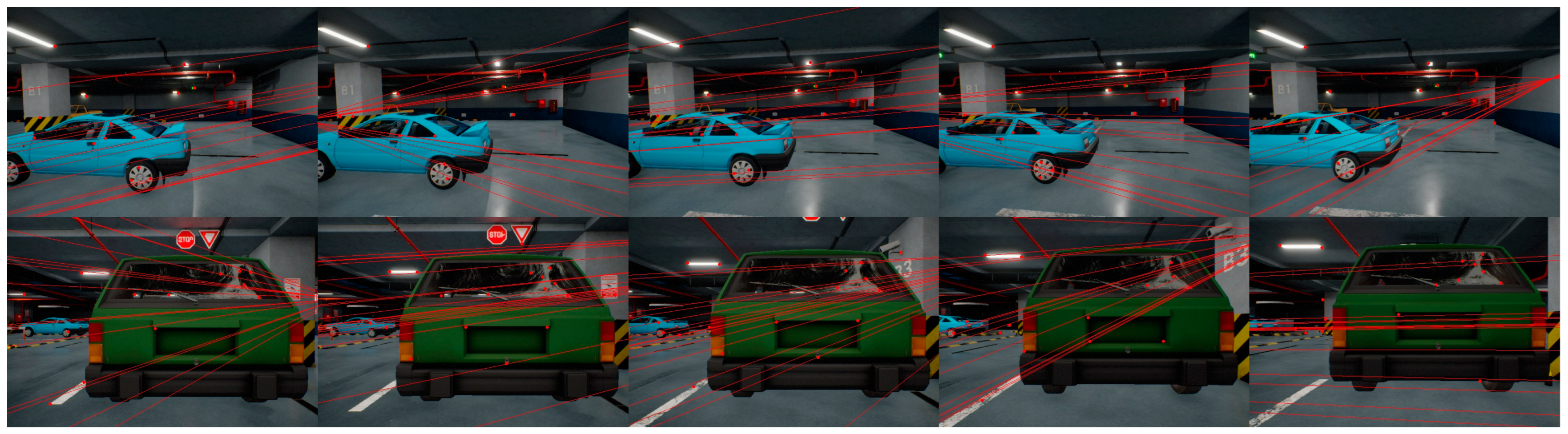
Figure 9.
Epipolar constraint results in the parking_lot 3_high sequence. The red lines indicate epipolar lines.
Figure 9.
Epipolar constraint results in the parking_lot 3_high sequence. The red lines indicate epipolar lines.

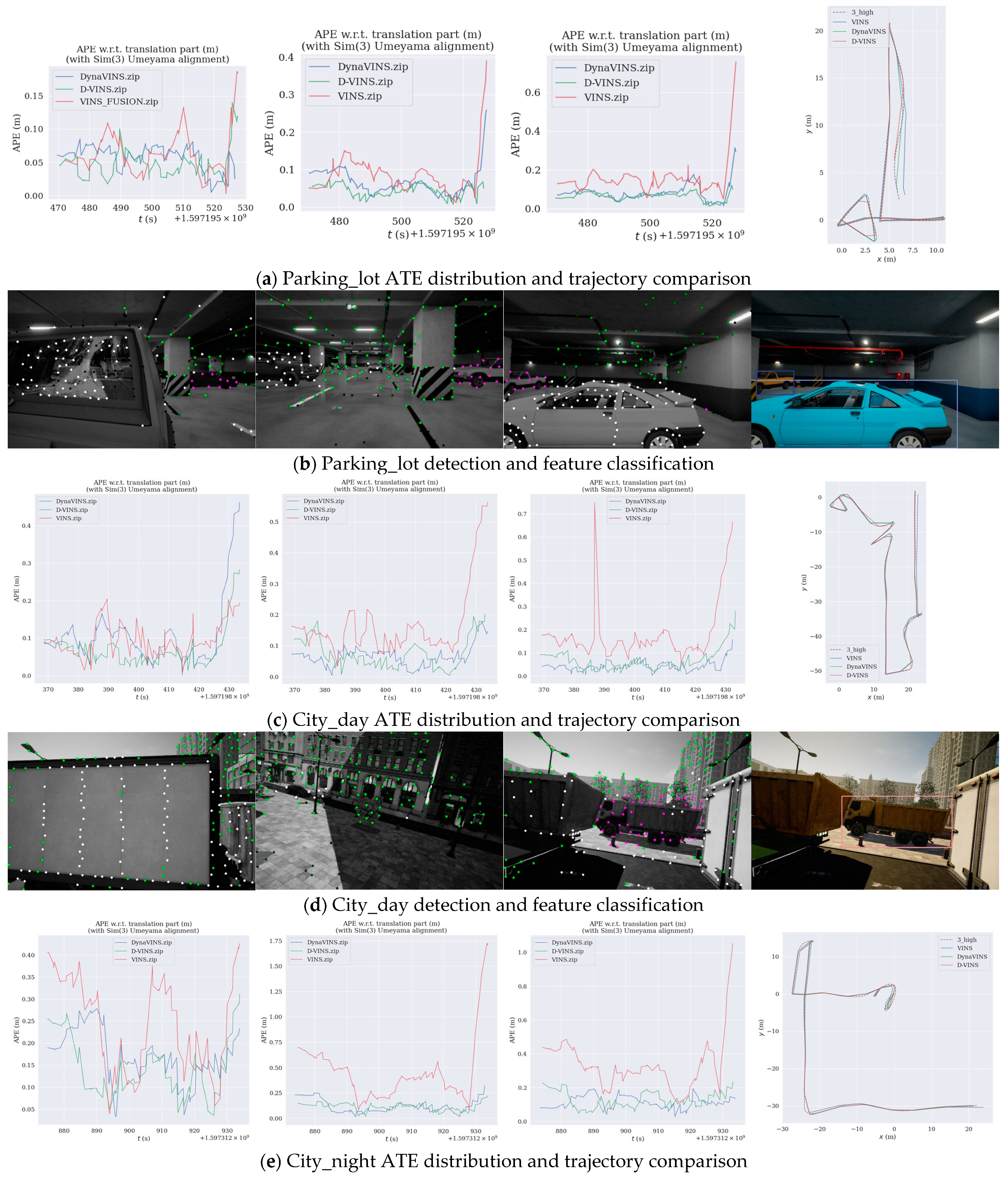
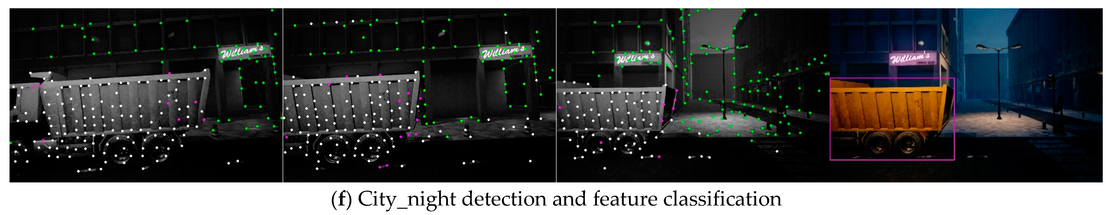
Figure 10.
Results of the trajectories and detection of VINS-Fusion, DynaVINS, and D-VINS on the VIODE dataset (parking_lot, city_day, and city_night scenes).In (a,c,e), the first three figures show the ATE distributions of the 0_none, 1_low, and 2_mid. The last figure shows the trajectories of the three algorithms in the 3_high sequence. In (b,d,f), the first three figures show the dynamics of the feature check result, where the green points are absolute static points, the purple points are temporary static points, and the white points are absolute dynamic points. The last figure shows the bounding box from YOLOV5.


Figure 11.
Handheld/backpack data collection equipment. (a) shows the overall equipment. (b) shows the handheld part. (c) shows the backpack part. (d,e) show the data collection work with different modes.
Figure 11.
Handheld/backpack data collection equipment. (a) shows the overall equipment. (b) shows the handheld part. (c) shows the backpack part. (d,e) show the data collection work with different modes.

Figure 12.
Feature classification results on our dataset. (a) shows the 5_SLAM_country_dynamic_loop_1 sequence. (b) shows the 14_SLAM_car_road_1 sequence. (c) shows the 18_SLAM_car_road_2 sequence. The features in white are absolute dynamic points, those in green are absolute static points, and those in purple are temporary static points.

Figure 13.
APE distribution results on our dataset. (a) shows the 5_SLAM_country_dynamic_loop_1 sequence. (b) shows the 14_SLAM_car_road_1 sequence. (c) shows the 18_SLAM_car_road_2 sequence. DynaVINS failed to provide estimations in the 14_SLAM_car_road_1 and 18_SLAM_car_road_2 sequences, so it was not compared in those sequences.

Figure 14.
The box plot of the running time in each part of D-VINS. The average time to process one frame is about 70.5 ms (14 Hz).
Figure 14.
The box plot of the running time in each part of D-VINS. The average time to process one frame is about 70.5 ms (14 Hz).


Table 1.
The ATE- and RPE-RMSE (m) of ORB-SLAM2, ORB-SLAM3, and D-VINS on the TUM RGB-D dataset.
| Sequences | ORB-SLAM2 | ORB-SLAM3 | D-VINS * (Ours) | Improvement | ||||
|---|---|---|---|---|---|---|---|---|
| ATE | RPE | ATE | RPE | ATE | RPE | ATE | RPE | |
| fr3_sitting_static | 0.0116 | 0.0152 | 0.0097 | 0.0060 | 0.0080 | 0.0114 | 17.53% | - |
| fr3_sitting_xyz | 0.0133 | 0.0199 | 0.0098 | 0.0086 | 0.0153 | 0.0179 | - | - |
| fr3_sitting_halfs | 0.0336 | 0.0124 | 0.0208 | 0.0080 | 0.0252 | 0.0122 | - | - |
| fr3_walking_static | 0.4121 | 0.0299 | 0.2450 | 0.0163 | 0.0069 | 0.0101 | 97.18% | 38.04% |
| fr3_walking_xyz | 0.8856 | 0.1255 | 0.5617 | 0.0267 | 0.0155 | 0.0182 | 97.24% | 31.84% |
| fr3_walking_rpy | 0.5987 | 0.0528 | 0.6841 | 0.0289 | 0.0422 | 0.0432 | 92.95% | - |
| fr3_walking_ half | 0.4227 | 0.0338 | 0.3212 | 0.0202 | 0.0216 | 0.0234 | 93.27% | - |
Note: Bold data indicate the best results. The symbol “*” indicates that D-VINS removed the module containing the IMU. The symbol “-” indicates that the algorithm showed no improvement.
Table 2.
The ATE- and RPE-RMSE (m) of D-VINS and the compared methods on the TUM RGB-D dataset.
| Sequences | DS-SLAM | RS-SLAM | Dynamic-VINS | D-VINS * (Ours) | ||||
|---|---|---|---|---|---|---|---|---|
| ATE | RPE | ATE | RPE | ATE | RPE | ATE | RPE | |
| fr3_walking_static | 0.0081 | 0.0102 | 0.0067 | 0.0099 | 0.0077 | 0.0095 | 0.0069 | 0.0101 |
| fr3_walking_xyz | 0.0247 | 0.0333 | 0.0146 | 0.0210 | 0.0486 | 0.0578 | 0.0155 | 0.0182 |
| fr3_walking_rpy | 0.4442 | 0.1503 | 0.1869 | 0.2640 | 0.0629 | 0.0595 | 0.0422 | 0.0432 |
| fr3_walking_half | 0.0303 | 0.0297 | 0.0425 | 0.0609 | 0.0608 | 0.0665 | 0.0216 | 0.0234 |
Note: Bold data indicate the best results. The symbol “*” indicates that D-VINS removed the module containing the IMU.
Table 3.
The ATE-RMSE (m) of VINS-Fusion, DynaVINS, and D-VINS on the KITTI dataset.
| Sequences | VINS-Fusion | DynaVINS | D-VINS |
|---|---|---|---|
| KITTI 05 | 1.913 | 12.4668 | 1.7631 |
| KITTI 07 | 2.1927 | 3.8006 | 2.1100 |
Note: bold data indicate the best results.
Table 4.
The ATE-RMSE (m) of VINS-Fusion, DynaVINS, and D-VINS on the VIODE dataset.
| Scenes | Sequences | VINS-Fusion | DynaVINS | D-VINS |
|---|---|---|---|---|
| Parking_lot | 0_none | 0.0774 | 0.0595 | 0.0538 |
| 1_low | 0.1126 | 0.0826 | 0.0472 | |
| 2_mid | 0.1174 | 0.0630 | 0.0396 | |
| 3_high | 0.1998 | 0.0982 | 0.0664 | |
| City_day | 0_none | 0.1041 | 0.1391 | 0.0882 |
| 1_low | 0.2043 | 0.0748 | 0.0912 | |
| 2_mid | 0.2319 | 0.0520 | 0.0864 | |
| 3_high | 0.3135 | 0.0743 | 0.0835 | |
| City_night | 0_none | 0.2624 | 0.1801 | 0.1561 |
| 1_low | 0.5665 | 0.1413 | 0.1221 | |
| 2_mid | 0.3862 | 0.1192 | 0.1395 | |
| 3_high | 0.7611 | 0.1519 | 0.1566 |
Note: bold data indicate the best results.
Table 5.
The ATE-RMSE (m) of VINS-Fusion, DynaVINS, and D-VINS on the real dataset.
| Sequences | VINS-Fusion | DynaVINS | D-VINS |
|---|---|---|---|
| 5_SLAM_dynamic_loop_1 | 0.657039 | 2.145493 | 0.654882 |
| 14_SLAM_car_road_1 | 37.31964 | - | 27.60877 |
| 18_SLAM_car_road_2 | 299.7889 | - | 151.2075 |
Note: “-” indicates that the method failed to estimate the camera pose. Bold data indicate the best results.
Table 6.
The ATE-RMSE (m) of D-VINS (G), D-VINS (S), and D-VINS (G + S) on the VIODE dataset.
| Scenes | Sequences | D-VINS (G) | D-VINS (S) | D-VINS (G + S) |
|---|---|---|---|---|
| Parking_lot | 0_none | 0.1000 | 0.0568 | 0.0538 |
| 1_low | 0.1196 | 0.0517 | 0.0472 | |
| 2_mid | 0.1126 | 0.0709 | 0.0396 | |
| 3_high | 0.1387 | 0.0702 | 0.0664 |
Note: Bold data indicate the best results.
Disclaimer/Publisher’s Note: The statements, opinions and data contained in all publications are solely those of the individual author(s) and contributor(s) and not of MDPI and/or the editor(s). MDPI and/or the editor(s) disclaim responsibility for any injury to people or property resulting from any ideas, methods, instructions or products referred to in the content. |
© 2023 by the authors. Licensee MDPI, Basel, Switzerland. This article is an open access article distributed under the terms and conditions of the Creative Commons Attribution (CC BY) license (https://creativecommons.org/licenses/by/4.0/).
Share and Cite
MDPI and ACS Style
Sun, Y.; Wang, Q.; Yan, C.; Feng, Y.; Tan, R.; Shi, X.; Wang, X. D-VINS: Dynamic Adaptive Visual–Inertial SLAM with IMU Prior and Semantic Constraints in Dynamic Scenes. Remote Sens. 2023, 15, 3881. https://doi.org/10.3390/rs15153881
AMA Style
Sun Y, Wang Q, Yan C, Feng Y, Tan R, Shi X, Wang X. D-VINS: Dynamic Adaptive Visual–Inertial SLAM with IMU Prior and Semantic Constraints in Dynamic Scenes. Remote Sensing. 2023; 15(15):3881. https://doi.org/10.3390/rs15153881
Chicago/Turabian StyleSun, Yang, Qing Wang, Chao Yan, Youyang Feng, Rongxuan Tan, Xiaoqiong Shi, and Xueyan Wang. 2023. "D-VINS: Dynamic Adaptive Visual–Inertial SLAM with IMU Prior and Semantic Constraints in Dynamic Scenes" Remote Sensing 15, no. 15: 3881. https://doi.org/10.3390/rs15153881
Note that from the first issue of 2016, this journal uses article numbers instead of page numbers. See further details here.