
Tropospheric Delay Parameter Estimation Strategy in BDS Precise Point Positioning
by
 ,
,
Zhimin Liu
1,
Yan Xu
1,
Xing Su
1,*,
Cuilin Kuang
2,
Bin Wang
3,
Guangxing Wang
4 and
Hongyang Ma
5
1
College of Geodesy and Geomatics, Shandong University of Science and Technology, Qingdao 266590, China
2
Geosciences and Info-Physics, Central South University, Changsha 410083, China
3
Shanghai Astronomical Observatory, Chinese Academy of Sciences, Shanghai 200030, China
4
School of Geography and Information Engineering, China University of Geosciences, Wuhan 430074, China
5
School of Geomatics Science and Technology, Nanjing Tech University, Nanjing 211816, China
*
Author to whom correspondence should be addressed.
Remote Sens. 2023, 15(15), 3880; https://doi.org/10.3390/rs15153880
Submission received: 30 June 2023
/
Revised: 1 August 2023
/
Accepted: 1 August 2023
/
Published: 4 August 2023
(This article belongs to the Special Issue New Progress in GNSS Data Processing Technology and Modeling)
Abstract
:Tropospheric delay (TD) parameter estimation is a critical issue underlying high-precision data processing for global navigation satellite systems (GNSSs). The most widely used TD parameter estimation methods are the random walk (RW) and piece-wise constant (PWC). The RW method can effectively track rapid variations of tropospheric delay, but it may introduce excessive noise. In contrast, the PWC method introduces less noise, but it is less adaptable to cases of large variations of tropospheric delay. To address the problem of how to choose the optimal TD parameter estimation method, this paper investigates the variation patterns of international GNSS service zenith tropospheric delay (IGS ZTD) products and proposes a combined strategy model for TD parameter estimation. Firstly, this paper avoids the day-boundary jumps problem of IGS ZTD products by grouping based on single-day data. Secondly, this paper introduces discrete point areas (DPAs) to measure the magnitude of the ZTD values and uses comprehensive indicators to reflect the variation of ZTD. Next, based on the Köppen-Geiger climate classification, this study selected five different climate classifications with a total of 20 IGS stations as experimental data. The data assessed span from day of year (DOY) 001 to DOY 365 in 2022. This paper then applied 26 different parameter estimation strategies for static precise point positioning (PPP) data processing, and the parameter estimation strategies that were used include the RW and PWC (with the piece-wise constant ranging from twenty minutes to five hundred minutes at twenty-minute intervals). Finally, ZTD and positioning results were obtained using various parameter estimation methods, and a combined strategy model was established. We selected five different climate classifications of IGS stations as validation data and designed three sets of comparative experiments: RW, PWC120, and the combined strategy model, to verify the effectiveness of the combined strategy model. The experimental results revealed that: RW and the combined strategy model have a comparable ZTD accuracy and both are superior to PWC120. The combined strategy model improves the positioning accuracy in the U direction compared to RW and PWC120. In arid (B) and polar (E) regions with a small variation of TD, the PWC120 strategy displayed a better positioning accuracy than the RW strategy; in equatorial (A) and warm-temperate (C) regions, where there are large variations of TD, the RW strategy exhibited a better positioning accuracy than the PWC120 strategy. The combined strategy model can flexibly select the optimal parameter estimation method according to the comprehensive indicator while ensuring ZTD estimation accuracy; it enhances positioning accuracy.
1. Introduction
The electromagnetic wave signal of the global navigation satellite systems (GNSSs) can be decelerated through the effects of atmospheric molecules when traversing the atmosphere, causing signal propagation delay. This delay is termed atmospheric delay. Atmospheric delay consists of ionospheric delay and tropospheric delay (TD) [1,2]. TD can be split into hydrostatic delay (HD) and wet delay (WD) components [3,4,5]. HD, also called dry delay, is mainly affected by atmospheric pressure and temperature, contributing to about 90% of the total delay, and is relatively stable and can be corrected precisely using tropospheric models. WD is induced by water vapor in the atmosphere, accounting for about 10% of the total delay [6]. While WD varies considerably with water vapor distribution in space and time, it still cannot be neglected in high-precision GNSS data processing and is usually estimated as an unknown parameter.
Tropospheric delay is one of the most important sources of error that affects precise point positioning (PPP), and it is also an important parameter reflecting the atmospheric environment and climate phenomena. The accuracy of tropospheric delay estimation not only affects the positioning accuracy, but also directly relates to the reliability of GNSS meteorology inversion precipitable water vapor (PWV) [7,8,9]. To this end, researchers have proposed many methods to deal with tropospheric delay, of which the following two are frequently applied in PPP: model correction method and parameter estimation method. The model correction method has been previously used to establish a mathematical model to correct tropospheric delay based on the physical characteristics of the troposphere and the functional relationship between meteorological parameters that affect its characteristics and tropospheric delay [10,11]. The model correction method can be divided into two types: one is the traditional tropospheric model based on early radio sounding observations, such as the Saastamoinen model, Hopfield model, and Black model, etc. [12,13,14]. Traditional models require the input of measured meteorological parameters, such as the air pressure, temperature, and water vapor pressure, to calculate the zenith tropospheric delay (ZTD), with correction accuracy reaching the centimeter level. However, most international GNSS service (IGS) stations are not equipped with meteorological sensors, which hinders the real-time acquisition of meteorological parameters, including the pressure, temperature, and water vapor pressure near the station, and limits the use of traditional models. The other type consists of empirical models that do not require measured meteorological parameters, such as the GPT (global pressure and temperature) series, UNB (University of New Brunswick) series, GZTD, IGGtrop, SHAtrop, and EGNOS (European geostationary navigation overlay service) series of meteorological empirical models [15,16,17,18,19,20,21,22,23,24,25]. These models use a large amount of radiosonde observations data or numerical weather model (NWM) data to establish the empirical relationship between the tropospheric parameters and the time (DOY) and location at the global or regional scale. With the continuous improvement of these meteorological empirical models, some scholars have combined meteorological empirical models with zenith tropospheric delay models, such as the GPT3 + Saastamoinen method, which calculates the average deviation of ZTD at more than 16,000 global stations over 10 years at around −0.99 cm [26]. At present, some scholars have also combined numerical reanalysis data with tropospheric delay models and have achieved good results in improving the accuracy of prior values in precise models and in improving the positioning accuracy as well [7,27,28,29,30,31,32,33,34].
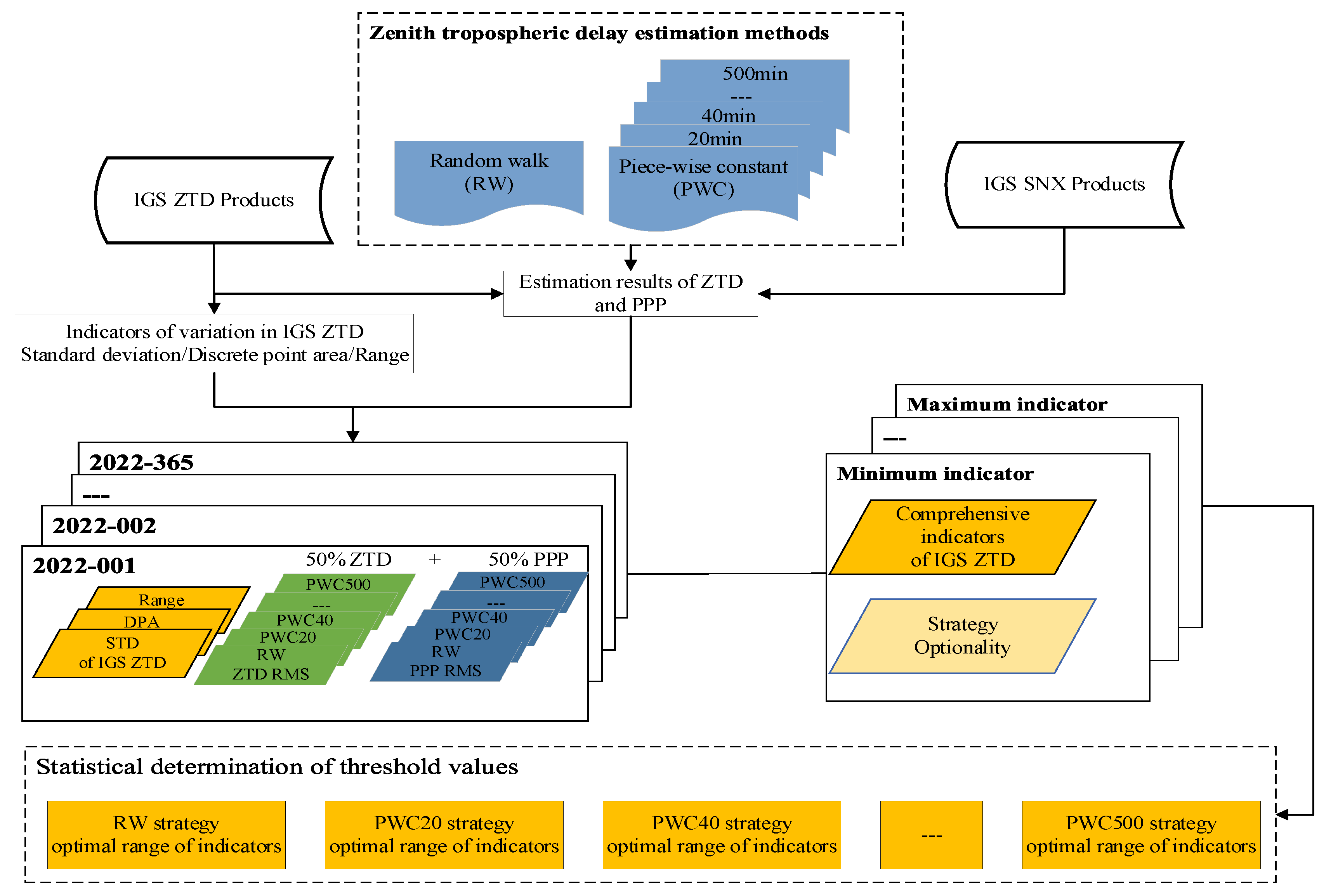
In the process of PPP computation, the zenith wet delay (ZWD) is usually estimated together with other unknown parameters using the least squares estimation. To estimate the ZWD accurately, it is usually necessary to adopt an appropriate parameter estimation strategy. At present, there are three common tropospheric delay parameter estimation strategies: piece-wise linear (PWL), piece-wise constant (PWC), and random walk (RW). Different tropospheric parameter estimation strategies have different impacts on the PPP accuracy. The PWC and PWL strategies divide the tropospheric delay into several time intervals and estimate a wet delay constant or linear parameter for each interval. The PWC strategy assumes that the estimated wet delay parameters are identical in the same interval, while the PWL strategy assumes that the estimated wet delay parameters vary linearly in the same interval. The PWC method has been widely applied in PANDA and PPP-AR ver. 2.2.6 software [35,36]; the PWL method has been applied in GAMIT GNSS processing software. Bar-Sever et al. (1998) applied the piece-wise linear method (PWL:5), updating the wet delay parameter at five-minute intervals [37]. Li, P. et al. (2010) compared the effects of the PWC and PWL methods on estimating the ZWD in PPP, and their results showed that the PWL method was better than the PWC method [38]. The random walk process is a parameter estimation method based on statistical principles. It was first employed by David et al. (1990) to calculate the noise of the tropospheric delay process using water vapor radiometers and meteorological data, following which they applied it to the theory of the first-order Gaussian–Markov process [39]. The random walk method has been widely used across various PPP software and services, such as PANDA, PPP-AR, RTKLIB, PPPH, Bernese, etc. [35,36,40,41]. Tomasz H. et al. (2017) proposed an optimization model that adjusts the noise of the random walk process in real time based on meteorological conditions. Compared with the fixed random process noise, this model improved the estimated accuracy of the ZTD value by 10% [42]. Jorge M. et al. (2018) analyzed the accuracy of ZTD estimation using the random walk method in three online PPP services and three PPP software packages, and found that the ZTD values that were estimated using the online PPP services were more consistent with the ZTD products [43]. The random walk method can effectively track the rapid variations of tropospheric delay but may introduce excessive noise; the piece-wise constant method introduces less noise but exhibits poor adaptability in cases of large tropospheric delay variations. However, there is a lack of effective indicators as the basis for choosing the appropriate parameter estimation strategy. To address the problem of how to choose the optimal tropospheric delay parameter estimation method, this study utilized IGS ZTD products to analyze the variation patterns of ZTD and determined the optimal parameter estimation strategy based on its variation patterns. Specifically, this paper employed four indicators to describe the variation features of ZTD: discrete point area (DPA), standard deviation (STD), variation of discrete point area (VDPA), and range. The DPA reflects the magnitude of the ZTD values, while the STD, VDPA, and range reflect the variation of ZTD. To determine the optimal parameter estimation strategy for different threshold ranges, we applied RW and various PWC method (with piece-wise constants ranging from twenty to five hundred minutes at twenty-minute intervals) tropospheric delay estimation strategies to perform PPP data processing on IGS stations with different climate classifications. By analyzing the relationship between ZTD variation indicators and various strategy results, we were thus able to design parameter estimation strategies that were suitable for different threshold ranges.
This paper is organized as follows: Section 2 introduces the mathematical models and methods that were used in the experiments of this paper. Section 3 describes the experimental data and GNSS data processing procedure and explains the process that was used to establish the optimal parameter estimation combined strategy model. Section 4 outlines the parameter estimation strategies that were implemented for different thresholds and verifies the effectiveness of the combined strategy model through data testing. Section 5 and Section 6 present the discussion and conclusions, respectively.
2. Mathematical Models and Methods
This section introduces the mathematical model of precise point positioning and the estimation methods and evaluation indicators of tropospheric delay, which lay the theoretical foundation for the subsequent data analysis.
2.1. Precise Point Positioning
Precise point positioning is a high-precision positioning method that utilizes precision ephemeris and clock products and corrects various errors through either model correction or parameter estimation. The first-order ionospheric delay that arises during the process of PPP is eliminated using the ionosphere-free (IF) combination. The functional model for the precise point positioning of the pseudo-range and carrier phase observations is as follows [44]:
where and are the carrier phase observations and pseudo-range observations, respectively. The superscript denotes the GNSS satellite and the subscript represents the receiver; and denote the wavelength and the ambiguity of the IF combination; and represents the geometric distance from the satellite to the receiver. and are the clock offsets at the receiver and satellite, respectively; refers to tropospheric delay; and denote the code and phase biases of the IF combination in the receiver end; and represent the code and phase biases of the IF combination in the satellite end; indicates the residual of the noise and multipath effects for the carrier phase observations; and signifies the residual of the noise and multipath effects for the pseudo-range observations.
2.2. Zenith Tropospheric Delay Computation
Tropospheric delay is usually computed through combining the model and parameter estimation methods. Firstly, the a priori values of the ZHD and ZWD are computed using the Saastamoinen model, and then the residual wet delay error is estimated using the parameter estimation method.
2.2.1. Tropospheric Delay Model
Each of the hydrostatic and wet parts of the tropospheric delay was mapped from the zenith direction to the elevation angle of the observation through the use of an elevation-dependent-only mapping function, the expression is as follows [45]:
where and are the mapping functions for the hydrostatic delay and wet delay, respectively, and is the elevation angle of the observation. is the zenith hydrostatic delay, which is typically calculated using the Saastamoinen model. is the zenith wet delay, which is usually calculated using the model to obtain the prior value . The remaining residuals were estimated using the least squares estimation. The Saastamoinen model can be written as follows [12]:
where P, T, and e represent the atmospheric pressure (hPa), temperature (K), and water vapor pressure (hPa) near the measuring station, respectively. φ and h denote the latitude (°) and altitude (m) of the station, respectively. In Equation (3), the meteorological parameters were provided using the GPT3 model with a spatial resolution of .
2.2.2. Tropospheric Wet Delay Parameter Estimation Method
In the static PPP solution process, the least squares filter is used to estimate the receiver coordinates, receiver clock bias, wet delay residuals, and ambiguity, with the wet delay residuals being implemented through a Gaussian–Markov process. The Markov process is a memory-less random process, in which the probability distribution of the current state is only related to the previous moment. This random process is called the random walk. The expression for the estimation of the wet delay parameter as a random walk process is as follows [39]:
where and represent the wet delay at time and t, respectively, the superscript s denotes the GNSS satellite, and the subscript r denotes the receivers. represents the wet delay residual, is the noise constraint of random walk between epochs, denotes the unit weight variance, represents the variance of wet delay residual, q is the power spectral density of noise, and represents the time interval between epochs [7]. In the estimation process of the tropospheric delay, the prior constraint of the model calculating the ZTD was set at 0.2 m while q was set at 0.0004 m.
The RW method estimates the ZWD based on the correlation between epochs, where t represents an epoch (in this study, the epoch interval was set at 30 s). The PWC method divides the entire observation time into multiple time periods based on a given constant, introducing a wet delay parameter for each time period. The residual wet delay estimated within the same period was the same. In this study, it was actually treated as a random walk process in between time periods, such as in the PWC120 strategy (the method of piece-wise constants which uses 120 min as the duration of each time segment), where is 120 min; for both the random walk and segmented constant methods to calculate, needs to be converted from minutes to hours.
2.3. Evaluation Indicators of Zenith Tropospheric Delay Value and Variation
The different methods of tropospheric delay parameter estimation will lead to different ZTD values and positioning accuracies, and the variation of ZTD is an important factor affecting its accuracy. In order to better reflect the value and variation of ZTD, we proposed several indicators to evaluate the ZTD. This section will introduce the variation indicators of tropospheric delay in detail, and use root mean square (RMS) as the evaluation criterion for positioning and ZTD accuracy.
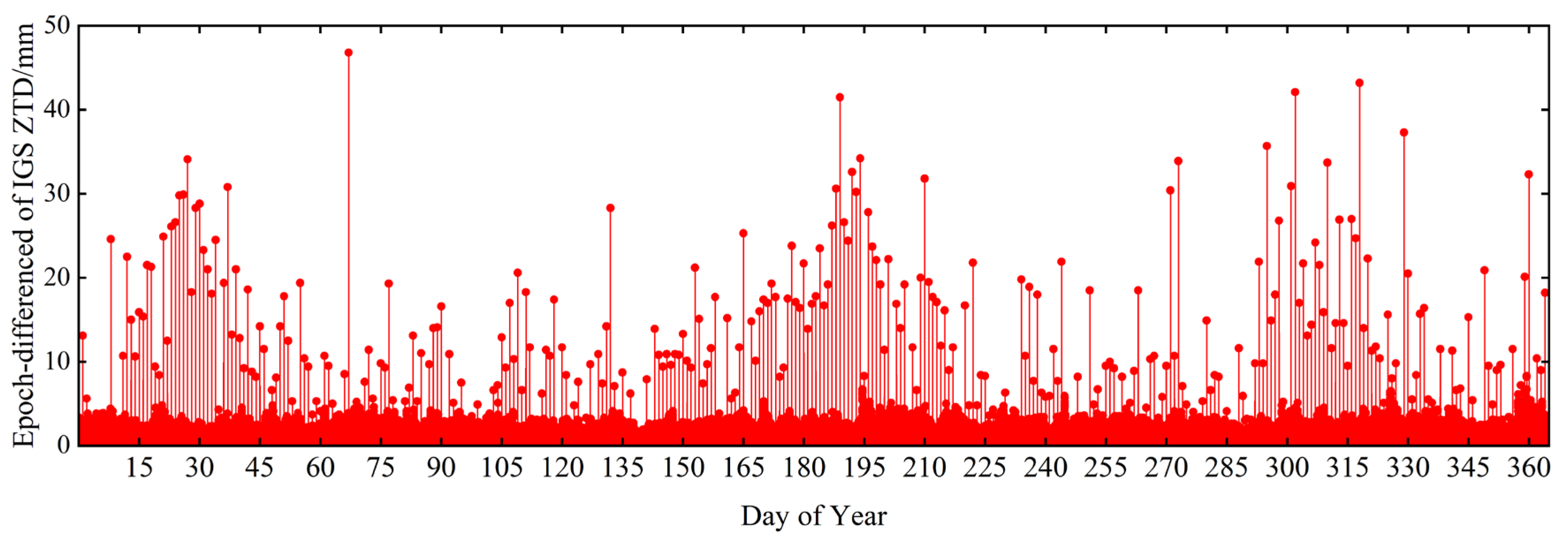
Figure 1 shows the epoch differences of IGS ZTD for the CRO1 station from DOY 001 to DOY 365 in 2022, which reveals that there is an obvious phenomenon of day-boundary jumps in the IGS ZTD product. This could have been due to the use of precise clock products with the day-boundary jumps problem when calculating the IGS ZTD [46]. To avoid the impact of the day-boundary jumps problem on the variation indicators of ZTD, we analyzed each day’s data as a group.
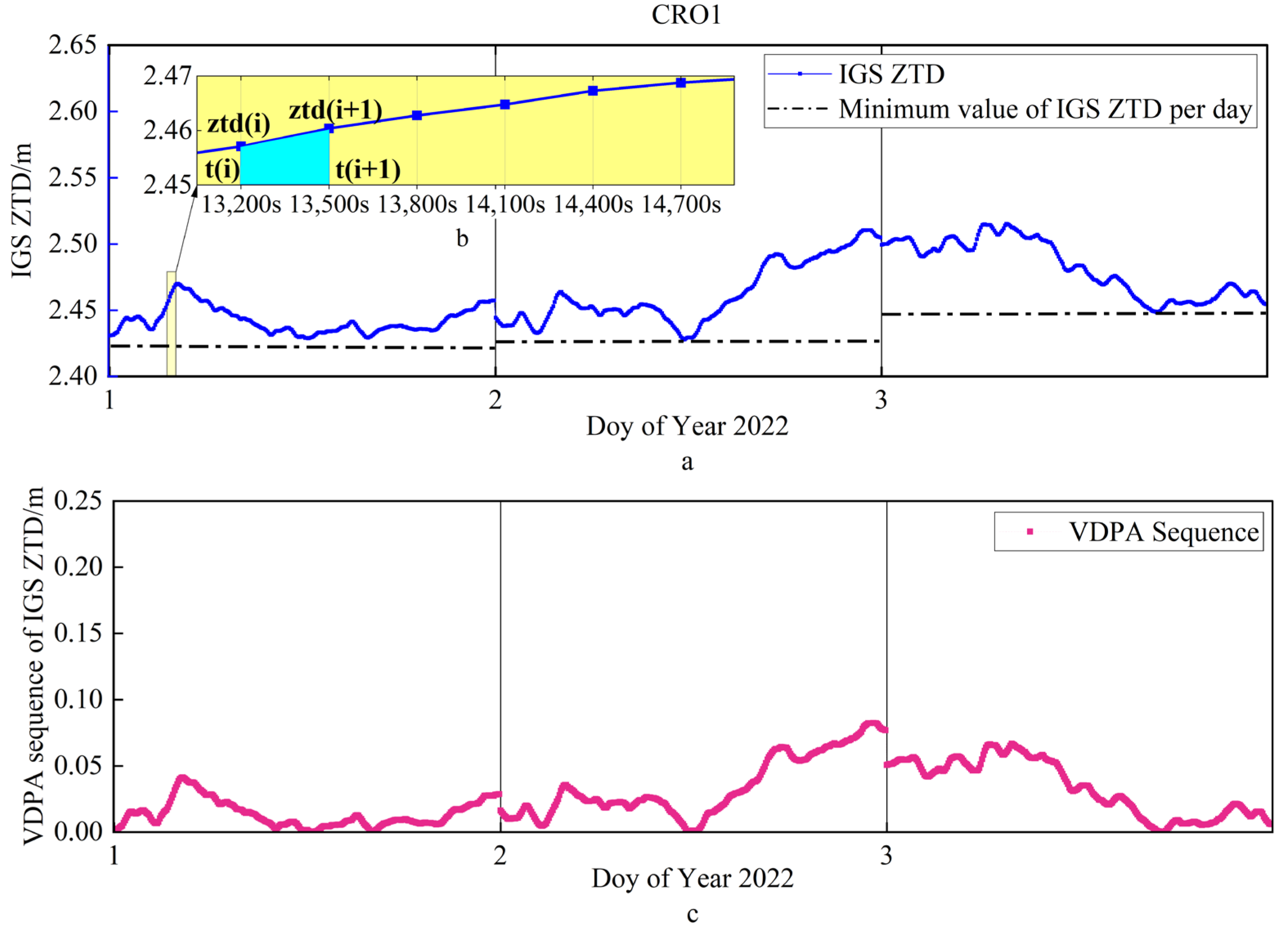
In order to accurately explain the meaning of the indicators that we have introduced in this study, we used the IGS ZTD data of the CRO1 station from DOY 001 to DOY 003 in 2022 as an example, as shown in Figure 2. In Figure 2a, the blue curve represents the IGS ZTD sequence with each epoch being 300 s, and the black dashed line represents the minimum value horizontal line in the daily IGS ZTD sequence. Figure 2b displays an enlargement of a certain area of the IGS ZTD, which was constructed in order to show the calculation process of our proposed discrete point area method more clearly; Figure 2c shows the IGS ZTD discrete point area sequence that was obtained using the improved discrete point area method.
Standard deviation (STD) can measure the absolute dispersion and fluctuation amplitude of the ZTD sequence. The larger the value of standard deviation, the more dispersed the ZTD, and the more violent the fluctuation of ZTD. The equation for std is as follows:
where is the ZTD value of epoch i, represents the daily mean of ZTD, and n denotes the total number of epochs in a single day.
The range is the difference between the maximum and minimum values in a set of data. The range method is suitable for situations where the data size is small. When the data size is large, the range method may ignore the overall trend of the variations of data. For the complex tropospheric delay, using the range method would be difficult for obtaining high-precision results. However, since this experiment analyzes each day’s data as a group, it improves the applicability of the range method. The equation for the Range is as follows:
where and are the maximum and minimum values of the single-day ZTD, respectively.
The discrete point area (DPA) refers to the trapezoid that is typically formed through connecting with [, , , ], as shown in Figure 2b. Using the trapezoidal rule for integration, we can thereby obtain the area between adjacent points. The sum of the discrete point areas for n epochs can then be calculated to represent the magnitude of daily ZTD changes, the equation for which is as follows:
where DPA is the sum of the epoch’s discrete point area, is the time of epoch i, and represents the ZTD value of epoch . This indicator can reflect the size of the ZTD value, but if the value of ZTD is large and changes slowly, the discrete point area calculated can also be large. Therefore, the discrete point area calculated in the above equation cannot evaluate the changes in ZTD. In order to improve the DPA, each ZTD value, , obtained in a single day (blue curve in Figure 2a) was subtracted by the minimum ZTD value, , in that day (as shown in the part above the black dashed line in Figure 2b); the improved IGS ZTD discrete point area series is displayed in Figure 2c. Following this step, the sum of the discrete point areas of n epochs was calculated to obtain the variation of discrete point area (VDPA), which can be used to evaluate ZTD changes. The equation is as follows:
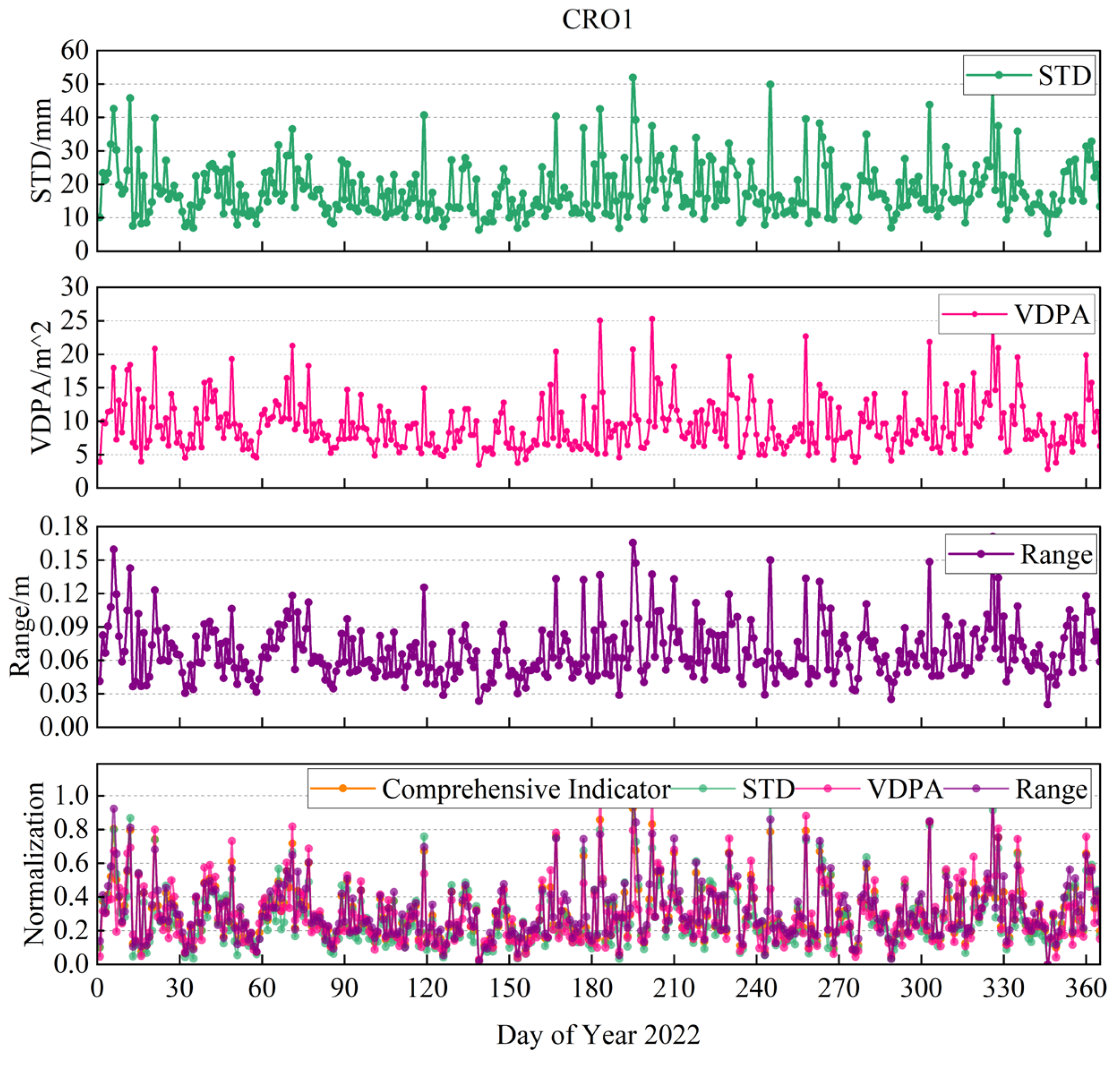
Taking the IGS ZTD of the CRO1 station from day 1 to day 365 in 2022 as an example in Figure 3, the three indicators mentioned above, namely the STD, VDPA, and range, were normalized for visual verification of their feasibility. The normalization equation is as follows:
where is the normalized value of within the range of [0:1]. and are the minimum and maximum values of the single-day ZTD, respectively. In this study, the calculation of these three normalized indicators serves as a comprehensive indicator itself for evaluating the changes in tropospheric delay, with the specific equation being as follows:
As shown in Figure 3, the variation trends of the three indicators STD, VDAP, and range are basically the same; the consistency between these three indicators after normalization was also high, and the comprehensive indicator also demonstrated a good consistency. This indicates that the comprehensive indicator that was constructed using the normalized standard deviation, discrete point area, and range of three indicators to evaluate the variation of tropospheric delay is feasible.
3. Data and Processing
This section explains the time period and distribution of the observation data selected, describes the static PPP data processing strategy in detail, and outlines the process of implementing the optimal parameter estimation combined strategy model in this study.
3.1. GNSS Data and Products
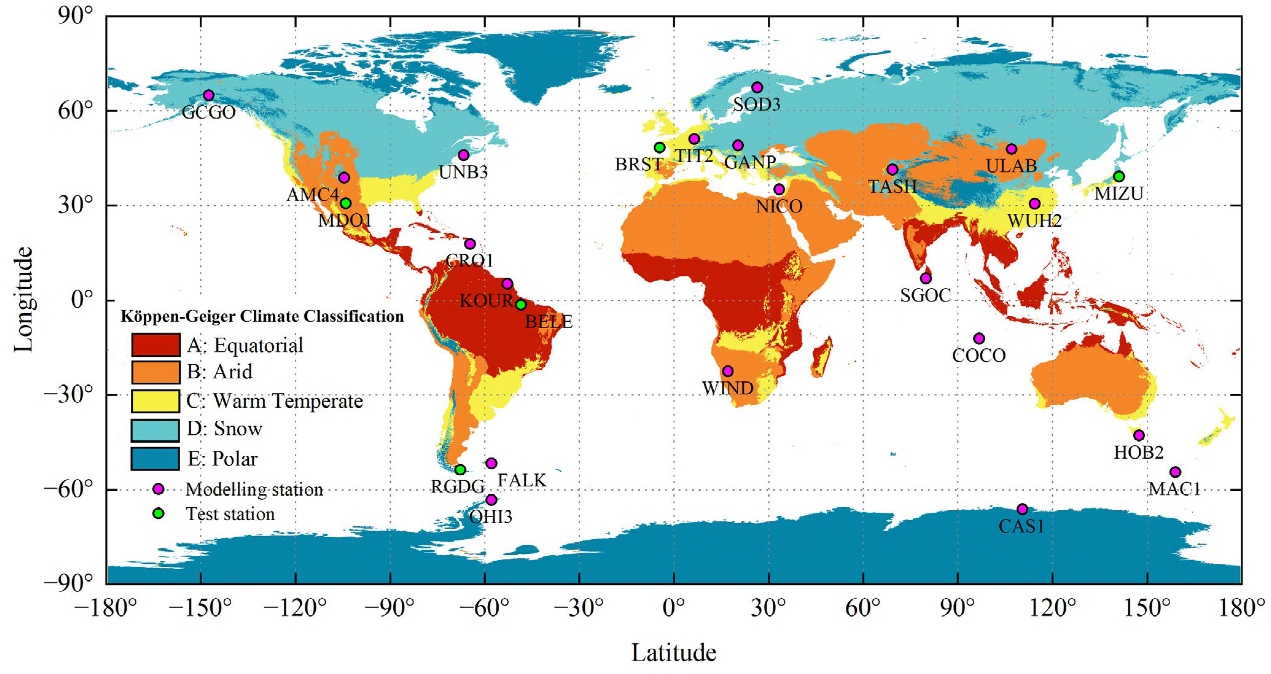
This study selected the observation data of 20 + 5 IGS stations distributed in different climate classifications around the world from DOY 001 to DOY 365 in 2022, among which twenty stations were used to build the model and five stations were used to verify the model. The station distribution is shown in Figure 4. The climate classifications are constantly improved based on the Köppen-Geiger climate classification. Currently, the world is divided into five climate regions based on the monthly and annual temperatures along with the precipitation in each region [47,48,49]. The climate classifications of each station are shown in Table 1.
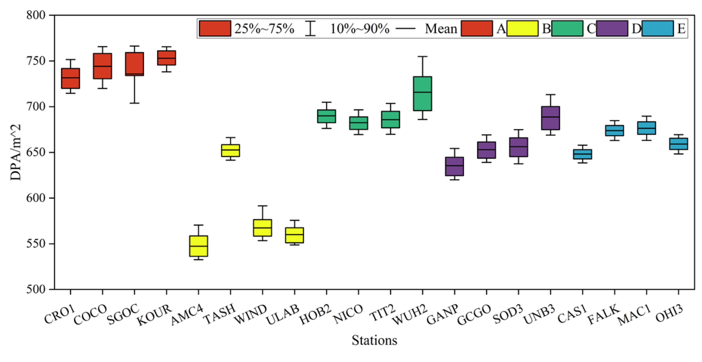
A certain correlation exists between tropospheric delay and climate classification. Climate classifications vary greatly across different regions and seasons, and these differences are often closely related to the temperature and precipitation in each region. Temperature and precipitation can directly affect factors, such as atmospheric pressure, temperature, and water vapor content, which are related to tropospheric delay. Figure 5 shows the time sequences of the IGS ZTD for five climate classifications. It can be seen from the figure that the equatorial region (A) exhibits a high temperature and rainfall throughout the year (corresponding to a high water vapor content) with a ZTD value between 2.4 m–2.7 m, which was noted as the largest among the five climate classifications. The arid region (B) has a hot and dry climate, and low water vapor content, and the ZTD ranges from approximately 1.8 m to 2.1 m. The TASH station is located at the junction of the B, C, D, and E classifications, and displays complex climatic characteristics. Therefore, the ZTD of this station was different compared to other B region stations. The warm-temperate region (C) has a mild climate and moderate rainfall, and their ZTD is generally distributed between 2.4 m–2.5 m. The region where the WUH2 station is located is greatly affected by the monsoon, especially in the summer, during which the precipitation increases (meaning the water vapor content increases), and the ZTD can reach around 2.7 m. The snow (D) and the polar (E) regions are generally cold and dry, leading to low ZTD values ranging between 2.1 m and 2.5 m. However, compared to the ZTD in classification D, the ZTD in classification E is relatively more stable. Figure 6 shows the DPA of the IGS ZTD for these five climate classifications; The DPA can also effectively reflect the numerical size of ZTD across these five climate classifications.
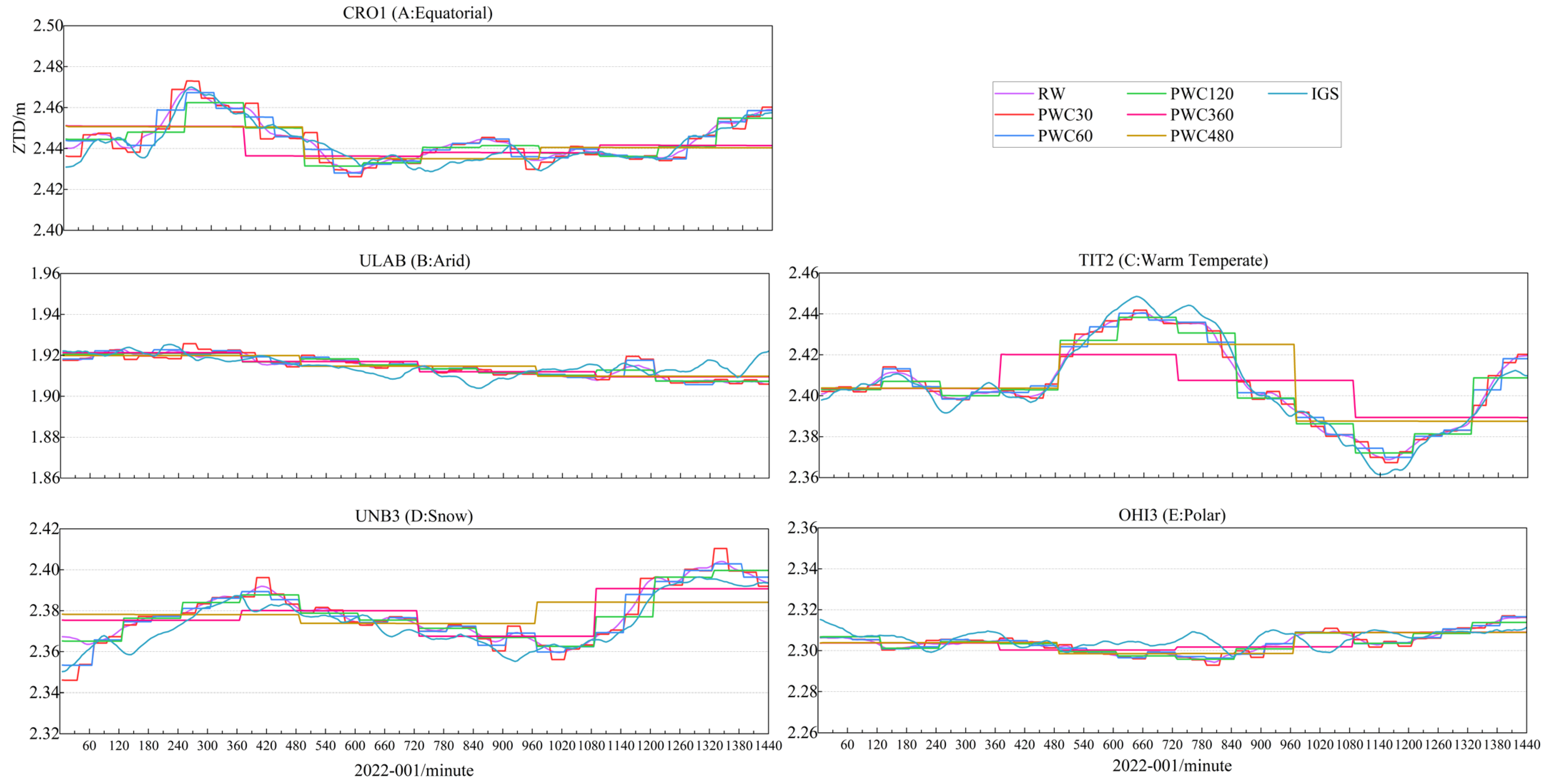
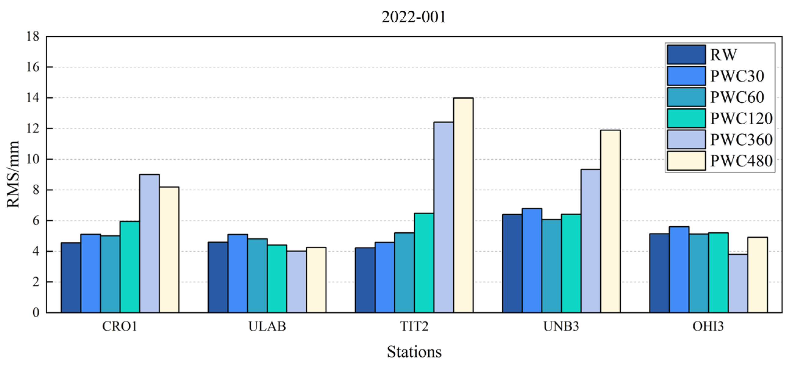
The variations of tropospheric delay are different across different climate classifications. When the tropospheric delay varies relatively smoothly, choosing a larger interval of the piece-wise constant strategy can effectively reduce the number of unknown parameters for least squares estimation and improve the stability of tropospheric delay estimation. When the tropospheric delay varies more sharply, choosing random walk or a smaller interval of the piece-wise constant strategy can update the tropospheric delay parameters frequently to adapt to the sharp variations of tropospheric delay and improve the accuracy of tropospheric delay estimation. Therefore, we should consider both the number of unknown parameters in least squares estimation and the stability and accuracy of the estimation results to choose a more suitable parameter estimation strategy. Figure 7 shows the ZTD estimation results and the IGS ZTD for five stations with different climate classifications using the RW, PWC30, PWC60, PWC120, PWC360, and PWC480 strategies on DOY 001 in 2022. Figure 8 shows the ZTD estimation accuracy for five stations with different climate types using the RW, PWC30, PWC60, PWC120, PWC360, and PWC480 strategies on DOY 001 in 2022. From Figure 7 and Figure 8, we can see that the tropospheric delay in the A (CRO1), C (TIT2), and D (UNB3) regions varied relatively largely within DOY 001, and that the adaptability and ZTD estimation results of the RW, PWC30, PWC60, and PWC120 parameter estimation methods with smaller intervals were significantly better than those of the PWC360 and PWC480 methods. In contrast, the tropospheric delay in the B (ULAB) and E (OHI3) regions varied only slightly within DOY 001, and the adaptability and ZTD estimation results of the PWC360 and PWC480 parameter estimation methods with larger intervals were found to be slightly better than those of the RW/PWC30/PWC60 and PWC120 methods.
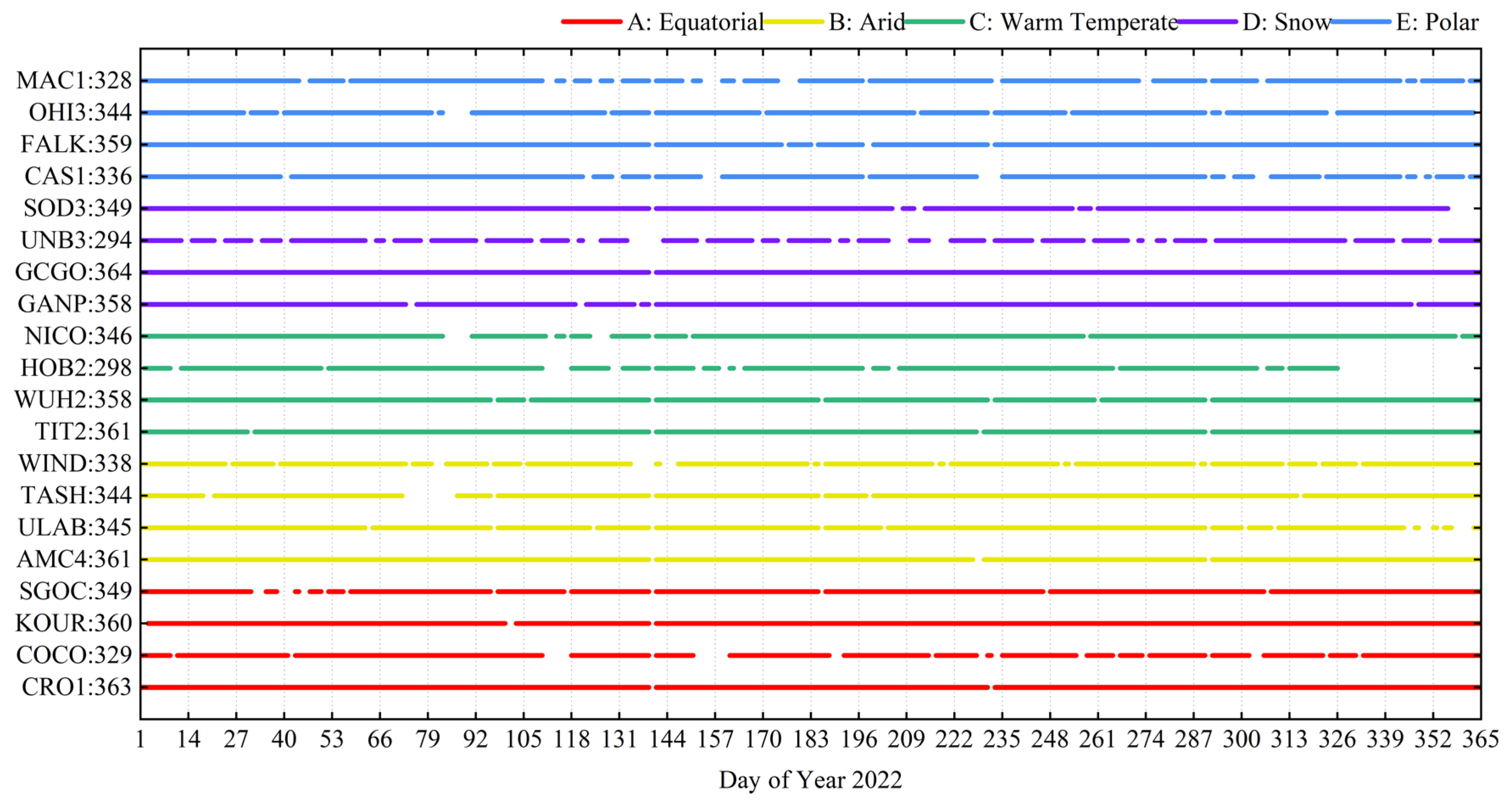
In order to evaluate the impact of RW and various PWC estimation strategies on ZTD accuracy and static PPP performance, we selected precise orbit and clocks products provided from WHU (ftp://igs.gnsswhu.cn/pub/whu/phasebias, accessed on 12 April 2023) to correct the satellite orbit and satellite clocks. After GNSS data processing, the positioning results select the international GNSS service standard network exchange (IGS SNX) solution products (ftp://igs.gnsswhu.cn/pub/gps/products, accessed on 12 April 2023) as the reference value for coordinates. For both the ZTD results and the variation indicators of ZTD, the IGS ZTD products (ftp://gdc.cddis.eosdis.nasa.gov/gnss/products/trop_zpd, accessed on 12 April 2023) were used. The IGS ZTD products have a time resolution of 300 s and an accuracy of around 4 mm [50]. Figure 9 shows the availability of data, where the horizontal axis represents the day of the year in 2022, and the vertical axis represents the stations and the total number of data used. These data will only be used when both the observation data and IGS ZTD products are available.
3.2. GNSS Data Processing
In terms of data processing, we used PRIDE PPP-AR, which was released by the GNSS Research Center of Wuhan University PRIDE Laboratory [36]. PPP-AR is an open source software that supports multi-satellite systems and multi-positioning modes. The various parameter estimation strategies explored in this study were also based on this software platform. The precise point positioning correction model includes antenna phase center and antenna phase center variation, phase wind-up effect, relativistic effect, solid earth tides, polar tides, ocean tides, etc. The parameters that were estimated in this study include receiver clocks, ambiguity, receiver coordinates, and the ZWD. Receiver clocks were estimated using the white noise method; ambiguity was resolved with the float solution strategy; and receiver coordinates were estimated as a constant. Table 2 displays the detailed GNSS data processing strategy.
4. Combined Strategy Model and Accuracy Analysis
In this section, we introduce in detail the implementation process of the optimal combined strategy model, and based on the optionality of strategies available, we recommend parameter estimation strategies within different ranges of indicators. After establishing the combined strategy model, we designed three sets of experiments, and used ZTD accuracy and PPP performance to verify the feasibility of the combined strategy model.
4.1. Combined Strategy Model
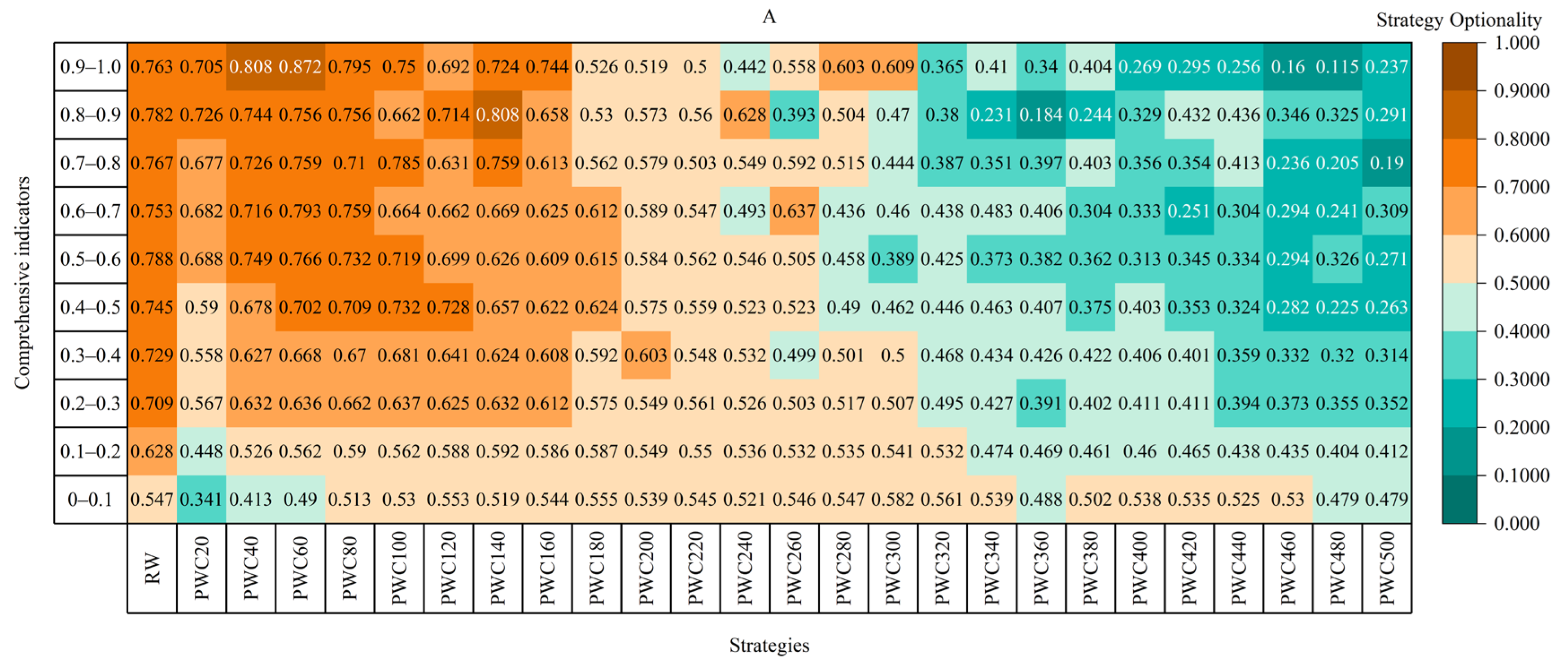
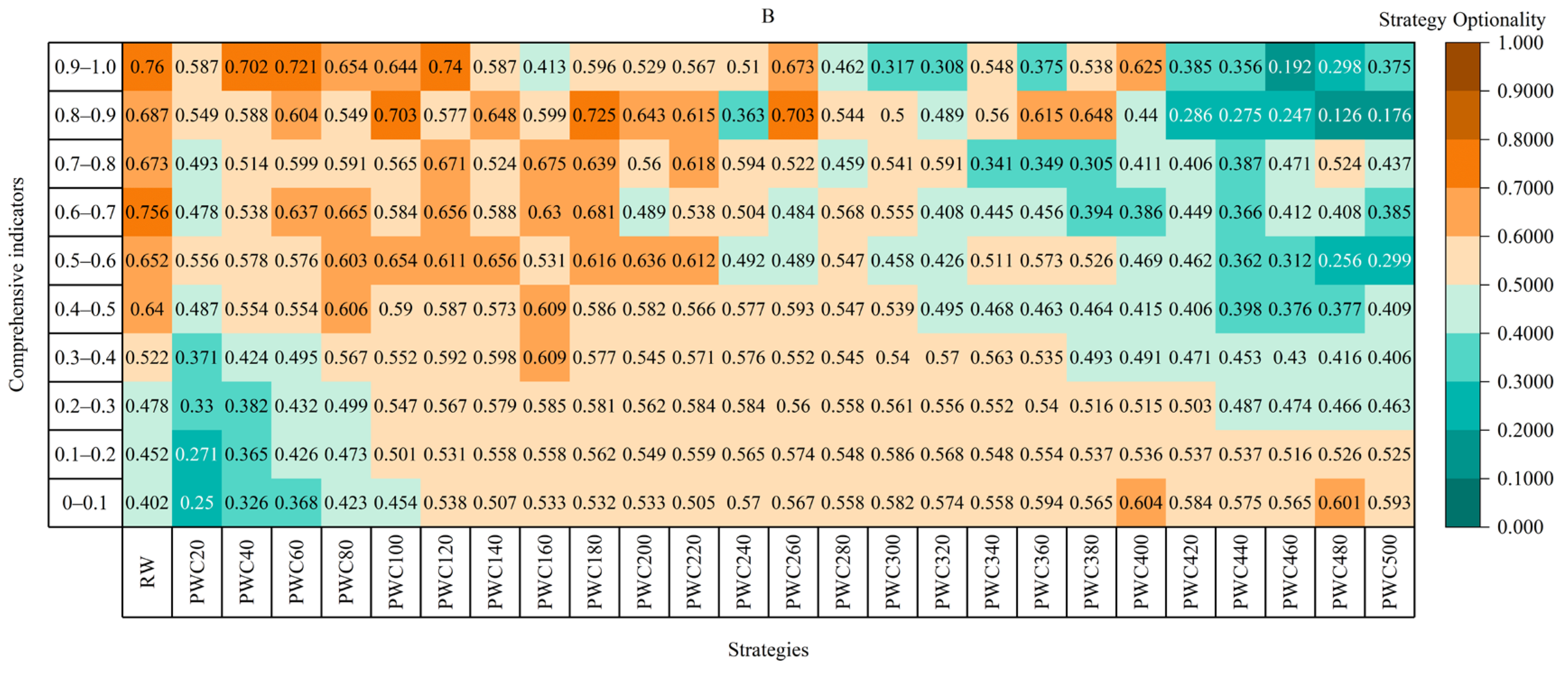
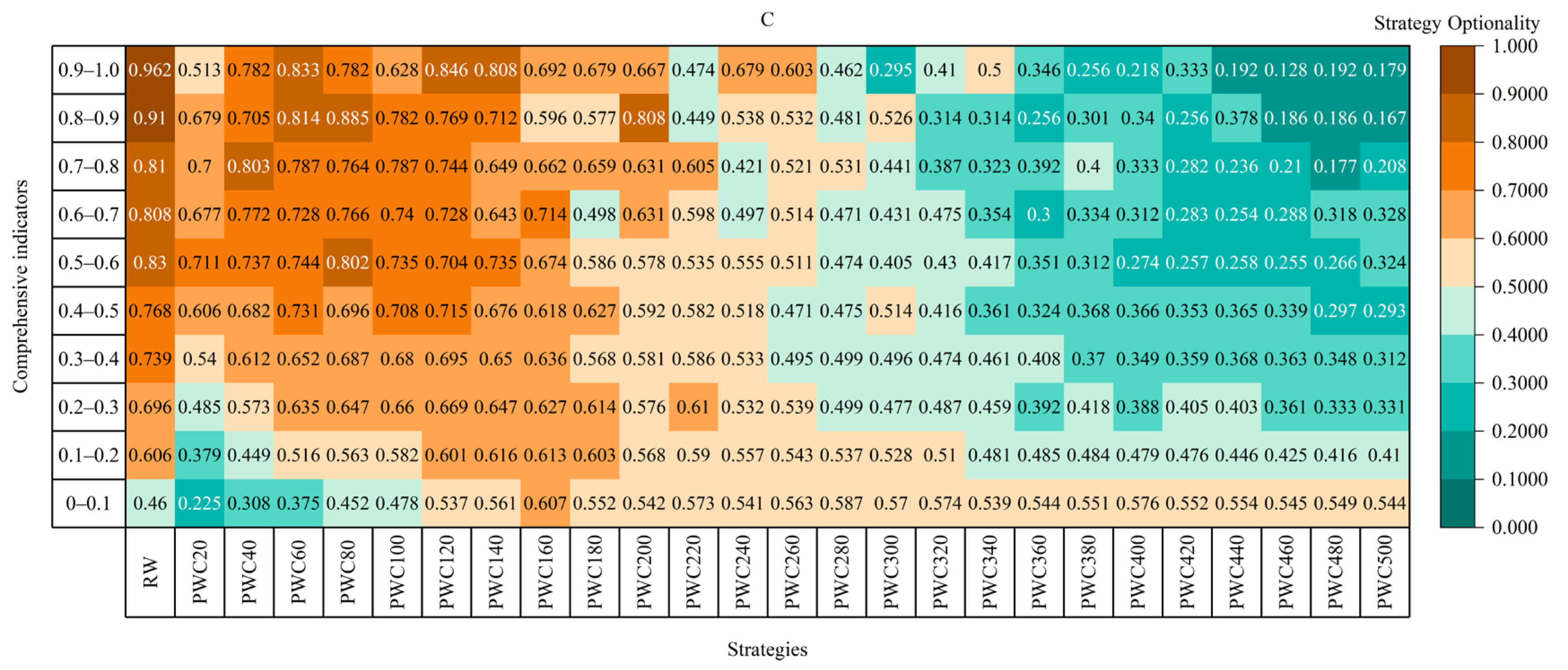
In order to establish the optimal tropospheric delay parameter estimation combined strategy model, we used RW and multiple PWC (PWC20/PWC40/…/PWC500—a total of 26) parameter estimation strategies for precise point positioning. The ZTD accuracy was calculated using the IGS ZTD products, and the accuracy of positioning (E/N/U) was calculated using the IGS SNX products as a reference. Considering the accuracy evaluation comprehensively, we used 50% of the U direction positioning accuracy and 50% of the ZTD accuracy to calculate the evaluation accuracy of the strategy. Next, we calculated the STD, range, and VDPA using Equations (7), (8), and (10), respectively, and normalized them. The comprehensive indicator was obtained using Equation (12). Assuming that these data were complete, we obtained 365 sets of data (including comprehensive indicator, RW precision, PWC20 precision, PWC40 precision,…, and PWC500 precision). Then, we sorted these 365 sets of data in ascending order according to the comprehensive indicator. In each set of data, we sorted the N (N = 26) kinds of parameter estimation strategy according to their accuracy to obtain the strategy s ranking position l within the indicator range, as well as its optional degree ; the specific equation is shown below. Ultimately, we obtained the optimal strategy corresponding to the comprehensive indicator’s threshold range. The technical roadmap is shown in Figure 10.
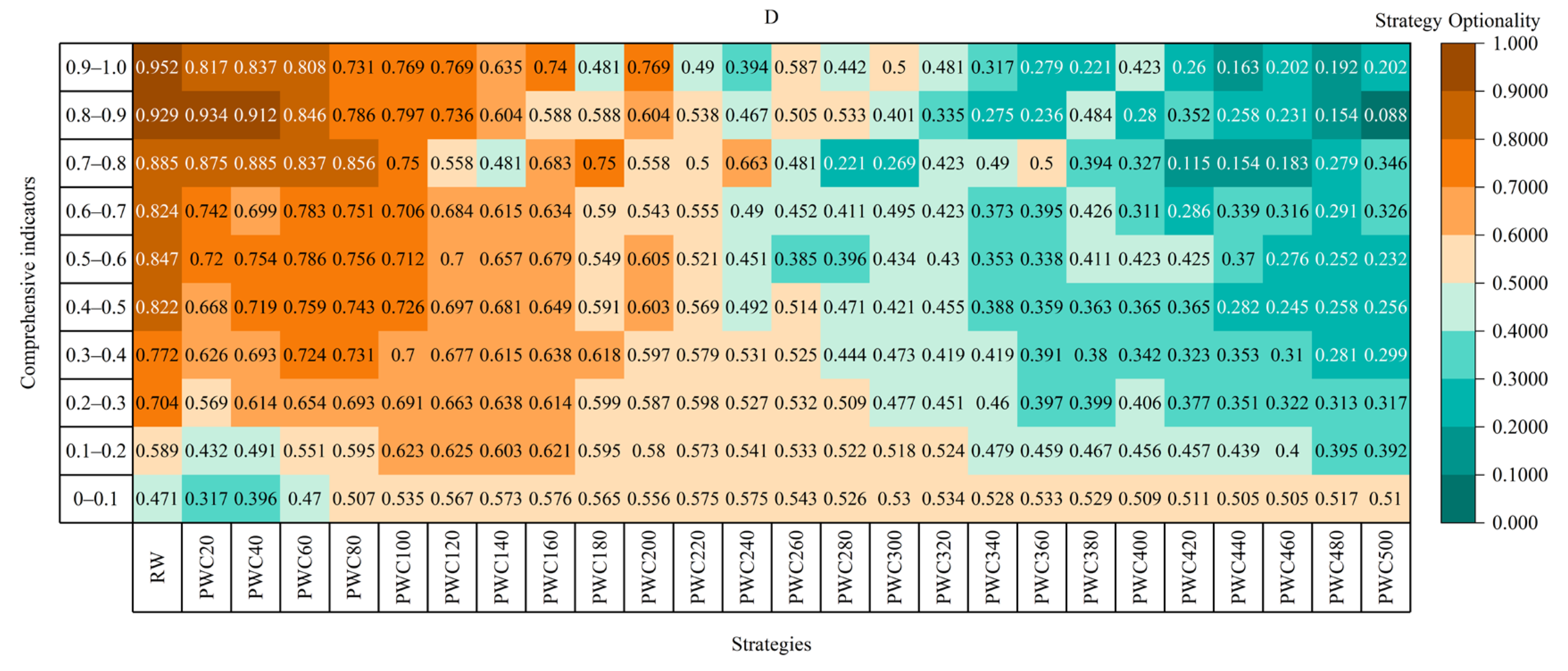
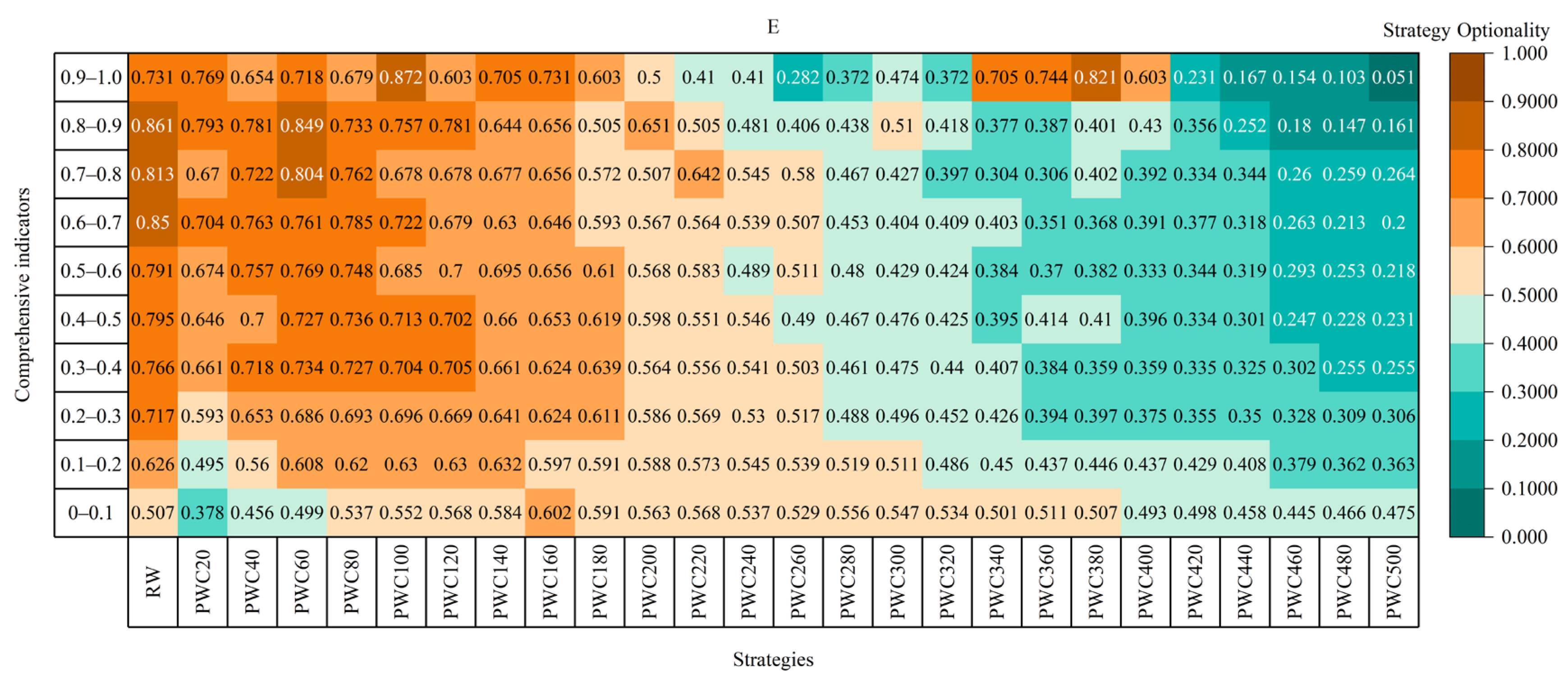
Figure 11, Figure 12, Figure 13, Figure 14 and Figure 15 demonstrate the optionality of these parameter estimation strategies within different threshold ranges in the equatorial region (A), arid region (B), warm-temperate region (C), snow region (D), and polar region (E), respectively. From these figures, it can be seen that the classifications of A, C, D, and E have relatively similar optional degrees of strategies, with highly optional degrees of strategies mainly concentrated before PWC200. However, the optionality of strategies for the classification of B appeared to be more dispersed. This phenomenon may be due to the influence of certain factors, such as the size of tropospheric delay and climate stability. Compared with the optionality of strategies for classifications A and E, the optionality of strategies for the classification of the C and D regions were more significantly concentrated prior to PWC120. This indicates that the RW estimation strategy is more suitable for the A, C, and D regions with unstable temperatures and precipitation. Although the optionality of strategies in the B classification was relatively dispersed, the optionality of strategies was generally concentrated before PWC120, when the comprehensive indicator was higher (with the IGS ZTD changing greatly). Based on the optionality of strategies in different threshold ranges, we recommended corresponding parameter estimation strategies for different threshold ranges, as shown in Table 3.
4.2. Combined Strategy Model Accuracy Analysis
To assess the enhancement effects of the combined strategy model on ZTD and positioning accuracy, we selected five stations with distinct climatic classifications from day 1 to day 365 of 2022, namely: BELE (A), MOD1 (B), BRST (C), MIZU (D), and RGDG (E). We devised three sets of experiments, including:
- PPP data processing employing the parameter estimation strategy of the combined strategy model;
- PPP data processing utilizing the random walk parameter estimation strategy;
- PPP data processing adopting the PWC120 parameter estimation strategy.
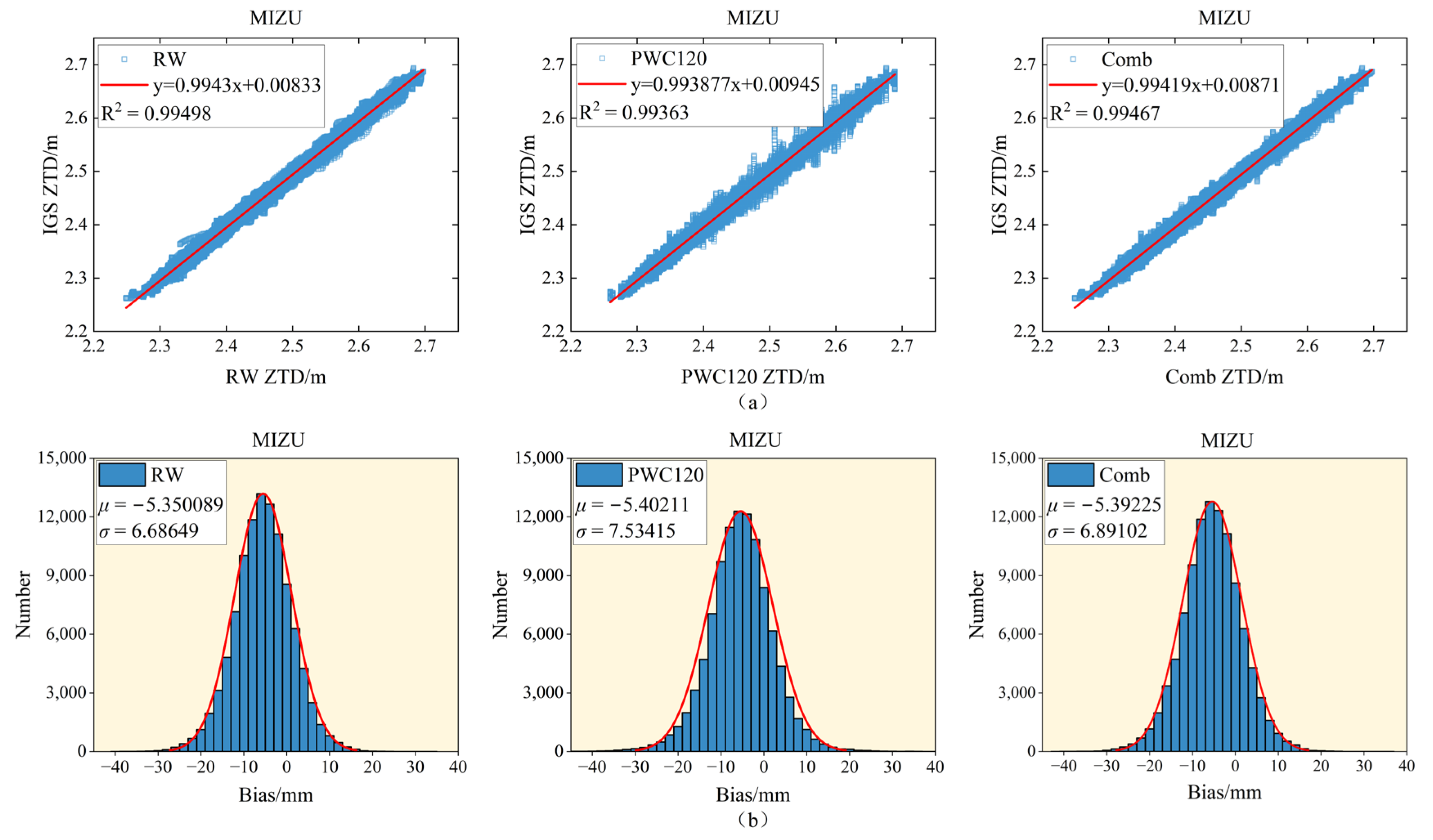
First of all, we analyzed the ZTD accuracy of these three strategies using the MIZU station as an example, subsequently presenting the PPP (E/N/U) and ZTD accuracy for all validation stations. Figure 16a illustrates the numerical relationship between the ZTD values estimated using the RW strategy, PWC120 strategy, and combined strategy model (abbreviated as Comb) and the IGS ZTD reference values at the MIZU station, where the red diagonal line indicates the fit line between the three parameter estimation strategies and the IGS ZTD. As shown in this figure, the fitting effects of the RW and Comb strategies were essentially consistent, while the PWC120 fitting effect was relatively inferior. Compared to the ZTD estimates of RW and Comb, the distribution of PWC120 ZTD estimates diverged more from the IGS ZTD reference values. The ZTD estimates of the RW and Comb strategies were evenly distributed and relatively concentrated on both sides of the fitting line compared to the PWC120-estimated ZTD values. Figure 16b displays the statistical distribution of ZTD errors for the RW, PWC120, and Comb parameter estimation strategies at the MIZU station, where the red curve represents the standard normal distribution curve (). According to Figure 16b, the and values of the RW and Comb strategies were closer to the standard normal distribution compared to the PWC120 strategy. Based on these analyses, the MIZU station exhibits a higher level of ZTD accuracy when using the RW and Comb strategy estimations.
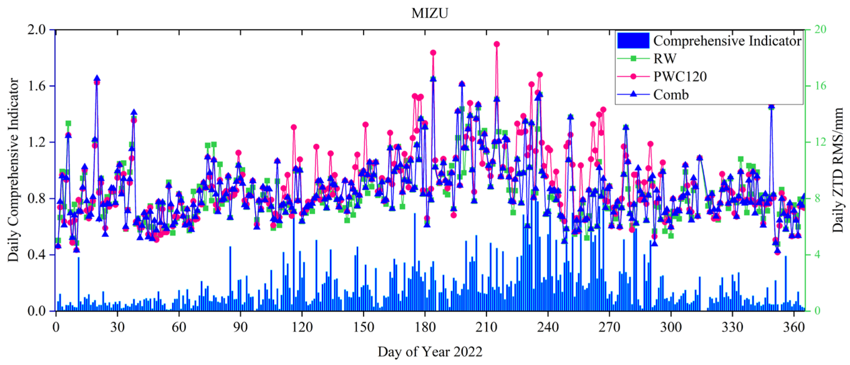
To further analyze the ZTD accuracy of the three strategies, we plotted the daily comprehensive indicator computed using the IGS ZTD and the daily ZTD accuracy of the RW, PWC120, and Comb strategies at the MIZU station, as shown in Figure 17. As shown in the figure, the comprehensive indicator values of the MIZU station significantly increased from DOY 230 to DOY 290. This is because during this period, the region where the MIZU station is located was, in the summer, influenced by the Pacific monsoon; rainfall increased (meaning that water vapor content also increased), resulting in drastic variations in the ZTD, thus increasing the value of the VDPA. Under the conditions of large comprehensive indicator values, the estimation accuracy of the RW and Comb strategies were found to be superior to the PWC120 strategy. Conversely, when the comprehensive indicator values were smaller, the PWC120 and Comb strategies exhibited a superior level of accuracy compared to the RW strategy. In conclusion, the combined strategy method can flexibly select the optimal strategy based on the magnitude of the comprehensive indicator, thereby achieving the goal of enhancing the ZTD and positioning accuracy.
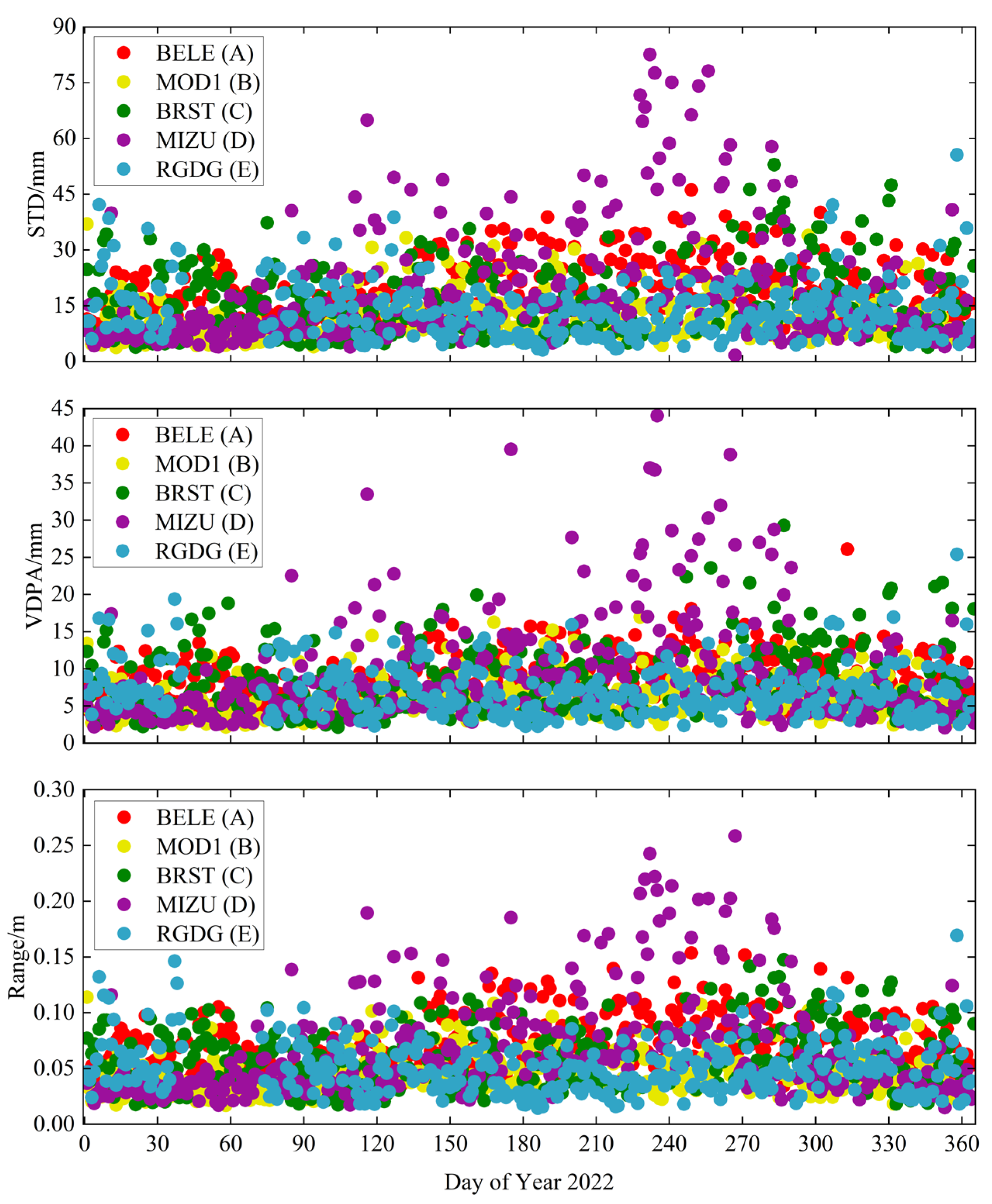
Figure 18 displays the STD, VDPA, and range of the IGS ZTD of all validation stations assessed in this experiment, with the purpose to illustrate the variations of the IGS ZTD. As shown in Figure 18, it is evident that the tropospheric delay fluctuations at the BELE station (A) and BRST station (C) were relatively intense, while the MIZU station (D) exhibited unstable variations in tropospheric delay. In contrast, the MOD1 station (B) and RGDG station (E) demonstrated comparatively minor variations of tropospheric delay. Regions in the A and C classifications experience perennial rainfall and higher water vapor content, resulting in further significant fluctuations of tropospheric delay. D regions are heavily influenced by seasonal factors, with smaller variations of tropospheric delay during the spring and winter seasons due to lower water vapor content, and larger variations of tropospheric delay during the summer and autumn seasons, when water vapor content increases. B and E exhibit smaller variations of tropospheric delay, as these regions are characterized by hot, arid, and cold, dry climates, respectively, leading to relatively stable atmospheric conditions, and resulting in the smaller variations of tropospheric delay.
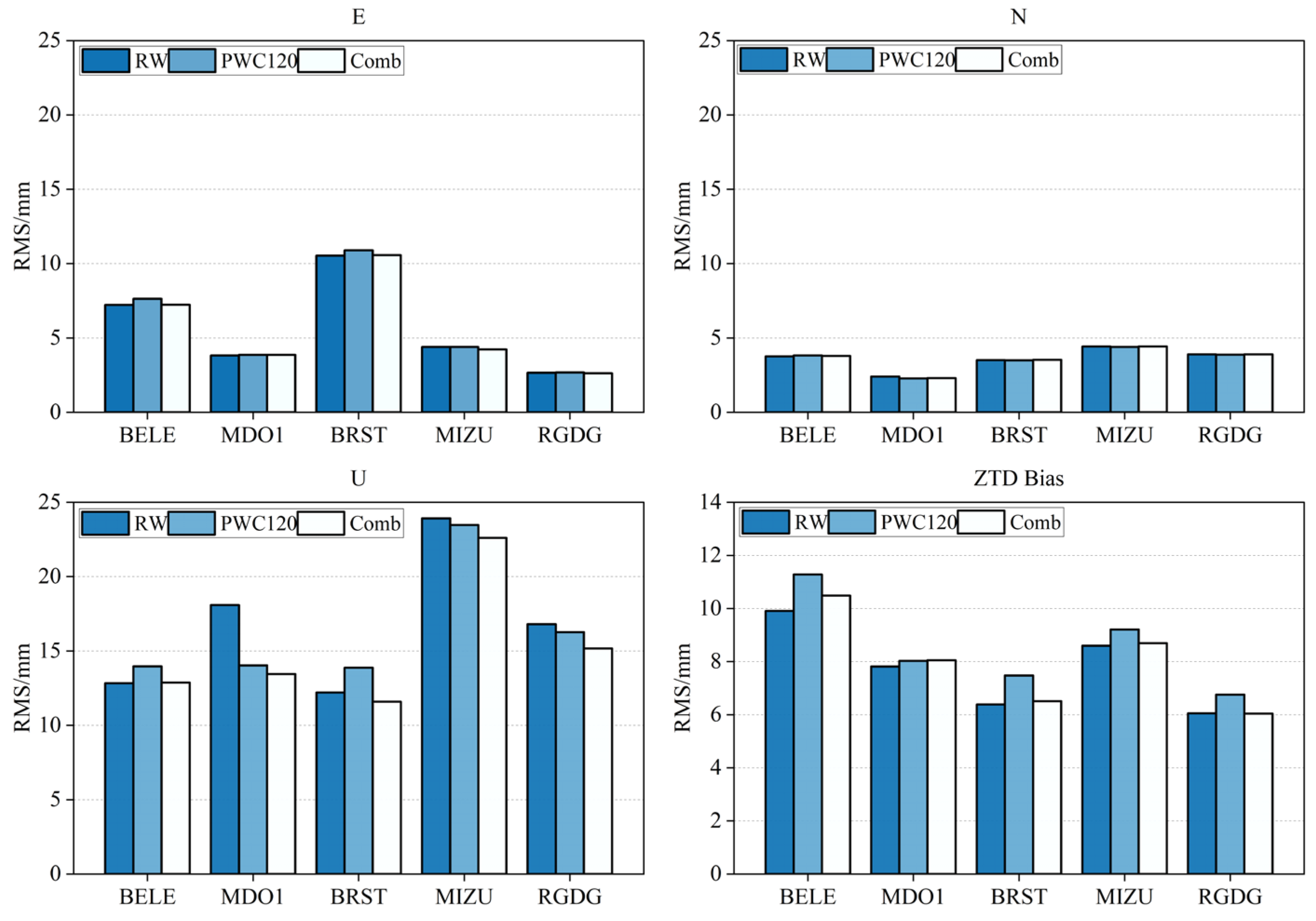
Figure 19 illustrates the PPP and ZTD accuracy for all validation stations, which were determined using the RW, PWC120, and Comb strategies. As shown in this figure, the positioning accuracy of the E and N directions of the three parameter estimation strategies was essentially consistent, which was because these three parameter estimation strategies mainly influenced the zenith tropospheric delay; the zenith tropospheric delay has a relatively minor impact on the E and N directions and exhibits relatively major impact on the U direction. Both the RW and Comb strategies exhibited a similar ZTD accuracy which surpassed that of the PWC120 strategy. This is because the RW strategy can frequently update the tropospheric delay parameters and has a high level of adaptability to any tropospheric delay variation situation. In contrast to the U directional positioning accuracies for the RW and PWC120 strategies, the Comb strategy demonstrated an enhanced positioning effect. In regions B and E, where the variation of tropospheric delay is small, the PWC120 strategy outperforms the RW strategy; meanwhile, in regions A or C, which are characterized with significant tropospheric delay fluctuations, the RW strategy outperforms the PWC120 strategy. In summary, the combined strategy model enhances the positioning accuracy while maintaining ZTD precision.
5. Discussion
The central concept of this study involves establishing a combined strategy model for different climatic classifications based on the ZTD and positioning results of 26 strategies. The threshold was determined using the comprehensive indicator range, while the optionality of the strategy relied on the ZTD and positioning accuracy. Figure 11, Figure 12, Figure 13, Figure 14 and Figure 15 illustrate the relationship between varying comprehensive indicators threshold ranges and the optionality of the strategy of 26 strategies. Drawing upon this optionality of strategy, we derived a combined strategy model, as presented in Table 3. To verify the precision of the combined strategy model, three sets of experiments were conducted. As shown in Figure 17 and Figure 19, the combined strategy model enhances the positioning accuracy while also maintaining the ZTD accuracy.
In PPP data processing, the selection of a tropospheric delay parameter estimation strategy is very important. The concept of the piece-wise constant method is to use fixed tropospheric delay parameters in each time interval. When the tropospheric delay variations are relatively stable, choosing a larger interval of the piece-wise constant strategy can effectively reduce the number of least squares unknown parameters, increase the constraint on other parameters, and enhance the accuracy of positioning. When the tropospheric delay variations are relatively drastic, choosing a random walk or smaller interval of the piece-wise constant strategy can frequently update the tropospheric delay parameters to adapt to drastic variations in the tropospheric delay, reduce the correction error of the tropospheric delay, and thus enhance the positioning accuracy. The combined strategy model selects the suitable parameter estimation strategy based on the variation of tropospheric delay. The combined strategy model can enhance the accuracy of positioning, but the enhancement effect of the combined strategy model on the accuracy of ZTD is not evident. According to the experimental results, choosing a random walk or smaller interval of the piece-wise constant method can achieve a higher accuracy of the ZTD. Therefore, if a higher positioning accuracy is required, we recommend using a combined strategy model; if a require higher ZTD accuracy is required, we suggest using a random walk. Moreover, in the PPP experiment, this paper adopts floating ambiguity rather than a fixed ambiguity technique. The main considerations are as follows: the aim of this paper was to assess the effect of different tropospheric delay parameter estimation methods on PPP positioning accuracy. Using floating-point ambiguity can eliminate the impact of the ambiguity resolution technique.
This study adopts a statistical perspective and applies various parameter estimation strategies for BDS PPP under different climate classifications. Based on the ZTD and positioning results of various strategies, an empirical model of combined strategy has been established. Based on this study, two aspects can be further explored. One aspect is from the perspective of the multi-satellite system. The research idea of the parameter estimation combined strategy model used in this paper is not only limited to BDS PPP, but can also be applicable to GPS PPP, GALILEO PPP, GLONASS PPP, and multi-system integrated PPP. Another aspect is from the perspective of climate classification refinement. The five climate categories outlined in this study can be further refined into more subcategories, such as the Mediterranean climate, temperate monsoon climate, and temperate maritime climate within the warm-temperate zone. These climates have different features. Mediterranean climate features hot and dry summers and mild and rainy winters; temperate monsoon climate areas are influenced by the monsoon during the summer with hot and humid weather along with cold and dry conditions in winter; the temperate maritime climate is moderated by the ocean with mild and rainy weather throughout the year. Therefore, using refined climate categories can establish a more accurate model of the combined strategy.
The combined strategy model used in this study is based on a daily basis. If the weather and environmental conditions vary significantly within a day, the applicability of this model may be limited. Therefore, it is very important to select the parameter estimation strategy and adjust the process noise according to the real-time situation.
6. Conclusions
To address the issue of how to select the appropriate method for tropospheric delay parameter estimating, this study proposed a combined strategy model that selects the optimal parameter estimation method based on the variations of the IGS ZTD. We first avoided the problem of day-boundary jumps in the IGS ZTD products displayed in Figure 1 through incorporating each day’s data as a group. Then, we introduced the DPA to indicate the size of the ZTD value and used the comprehensive indicator to measure the variation of ZTD. In order to link the comprehensive indicator of the IGS ZTD with different methods of tropospheric delay parameter estimation, we chose twenty stations (four stations for each climate type) according to five climate classifications and applied twenty-six parameter estimation methods (RW/PWC20/PWC40…PWC500) for static PPP data processing and obtained their ZTD values and positioning precision. This study came to the following conclusions:
- This study introduced the DPA and VDPA to assess the magnitude and variation of tropospheric delay, respectively. The DPA can accurately reflect the magnitude of the ZTD values, and the VDPA, STD, and range can all reflect the variations of ZTD. After normalization, there was a high agreement uncovered between the VDPA, STD, range, and the comprehensive indicator (derived from the three indicators).
- Tropospheric delay is related to climate classification. The equatorial region (A) is characterized with a high temperature and high precipitation (high water vapor content), and the ZTD value obtained was between 2.4 m and 2.7 m. The arid region (B) is marked by the hot and dry climate and low water vapor content, and their ZTD ranges from approximately 1.8 m to 2.1 m. The warm-temperate region (C) has moderate climate and rainfall, with their ZTD generally distributed between 2.4 m and 2.5 m. The snow region (D) and the polar region (E) have a cold and dry climate, which causes the production of a low ZTD value, mainly between the range of 2.1 m and 2.5 m; the ZTD of the E region is more consistent than that of the D region.
- The A, C, D, and E regions have similar optionality of parameter estimation strategies, with high optionality of strategies mainly concentrated before PWC200. However, the B region has a more scattered optionality of strategies. The A, C, and D regions have a more concentrated optionality of strategies than the B and E regions, which were mostly concentrated before PWC120. Even though the B region has relatively dispersed the optionality of strategies, it is also mostly concentrated before PWC120 when the comprehensive indicator is large (corresponding to the large variation of the IGS ZTD).
- Both the RW and combined strategy models exhibit a similar level of ZTD accuracy which surpasses that of the PWC120 strategy. This is because the RW strategy can frequently update the tropospheric delay parameters and has a high adaptability to any tropospheric delay variation situation.
- The combined strategy model improves the positioning accuracy of the U direction compared with the RW and PWC120 strategies. In B and E regions with the low variation of tropospheric delay, the PWC120 strategy has a higher accuracy of positioning than the RW strategy. In A and C regions with a high variation of tropospheric delay, the positioning accuracy of the RW strategy surpasses the PWC120 strategy. The combined strategy model can select the optimal parameter estimation strategy based on the comprehensive indicator, which enhances the accuracy of positioning while also maintaining the accuracy of ZTD.
Author Contributions
Conceptualization, X.S. and Z.L.; methodology, X.S. and Y.X.; software, Y.X.; validation, B.W., H.M. and G.W.; formal analysis, C.K. and B.W.; investigation, H.M.; resources, X.S. and G.W.; data curation, Y.X.; writing—original draft preparation, Y.X.; writing—review and editing, Z.L. and X.S.; visualization, Y.X.; supervision, Z.L.; project administration; funding acquisition, Z.L. All authors have read and agreed to the published version of the manuscript.
Funding
This work was sponsored by the Shandong Provincial Natural Science Foundation (Grant number ZR2023MD054); and the National Natural Science Foundation of China (Grant No. 42204036, 41904034).
Acknowledgments
We would like to thank the CDDIS (Crustal Dynamics Data Information System) for providing the IGS products and observation data (https://cddis.nasa.gov/archive/gnss/, accessed on 12 April 2023). We would also like to thank the Data Center of Wuhan University for providing precise ephemeris and clock bias products (ftp://igs.gnsswhu.cn/pub/whu, accessed on 12 April 2023).
Conflicts of Interest
The authors declare no conflict of interest.
References
- Chen, H.; Niu, F.; Su, X.; Geng, T.; Liu, Z.; Li, Q. Initial Results of Modeling and Improvement of BDS-2/GPS Broadcast Ephemeris Satellite Orbit Based on BP and PSO-BP Neural Networks. Remote Sens. 2021, 13, 4801. [Google Scholar] [CrossRef]
- Li, Q.; Su, X.; Xu, Y.; Ma, H.; Liu, Z.; Cui, J.; Geng, T. Performance Analysis of GPS/BDS Broadcast Ionospheric Models in Standard Point Positioning during 2021 Strong Geomagnetic Storms. Remote Sens. 2022, 14, 4424. [Google Scholar] [CrossRef]
- Zhang, S.; Fang, L.; Wang, G.; Li, W. The Impact of Second-Order Ionospheric Delays on the ZWD Estimation with GPS and BDS Measurements. GPS Solut. 2020, 24, 41. [Google Scholar] [CrossRef]
- Wang, G.; Bo, Y.; Yu, Q.; Li, M.; Yin, Z.; Chen, Y. Ionosphere-Constrained Single-Frequency PPP with an Android Smartphone and Assessment of GNSS Observations. Sensors 2020, 20, 5917. [Google Scholar] [CrossRef]
- Wang, G.; Yin, Z.; Hu, Z.; Chen, G.; Li, W.; Bo, Y. Analysis of the BDGIM Performance in BDS Single Point Positioning. Remote Sens. 2021, 13, 3888. [Google Scholar] [CrossRef]
- Yang, L.; Wang, J.; Li, H.; Balz, T. Global Assessment of the GNSS Single Point Positioning Biases Produced by the Residual Tropospheric Delay. Remote Sens. 2021, 13, 1202. [Google Scholar] [CrossRef]
- Lu, C.; Li, X.; Zus, F.; Heinkelmann, R.; Dick, G.; Ge, M.; Wickert, J.; Schuh, H. Improving BeiDou Real-Time Precise Point Positioning with Numerical Weather Models. J. Geod. 2017, 91, 1019–1029. [Google Scholar] [CrossRef]
- Singh, D.; Ghosh, J.K.; Kashyap, D. Precipitable Water Vapor Estimation in India from GPS-Derived Zenith Delays Using Radiosonde Data. Meteorol. Atmospheric Phys. 2014, 123, 209–220. [Google Scholar] [CrossRef]
- Wei, J.; Shu, Y.; Liu, Y.; Fang, R.; Qiao, L.; Ding, D.; Li, G.; Liu, J. Retrieving Accurate Precipitable Water Vapor Based on GNSS Multi-Antenna PPP With an Ocean-Based Dynamic Experiment. Geophys. Res. Lett. 2023, 50, e2023GL102982. [Google Scholar] [CrossRef]
- Ma, H.; Zhao, Q.; Verhagen, S.; Psychas, D.; Dun, H. Kriging Interpolation in Modelling Tropospheric Wet Delay. Atmosphere 2020, 11, 1125. [Google Scholar] [CrossRef]
- Ma, H.; Li, R.; Tao, J.; Zhao, Q. BDS PPP-IAR: Apply and Assess the Satellite Corrections from Different Regional Networks. Measurement 2023, 211, 112582. [Google Scholar] [CrossRef]
- Saastamoinen, J. Atmospheric Correction for the Troposphere and Stratosphere in Radio Ranging Satellites. In Geophysical Monograph Series; Henriksen, S.W., Mancini, A., Chovitz, B.H., Eds.; American Geophysical Union: Washington, DC, USA, 2013; pp. 247–251. ISBN 978-1-118-66364-6. [Google Scholar]
- Hopfield, H.S. Two-Quartic Tropospheric Refractivity Profile for Correcting Satellite Data. J. Geophys. Res. 1969, 74, 4487–4499. [Google Scholar] [CrossRef]
- Black, H.D. An Easily Implemented Algorithm for the Tropospheric Range Correction. J. Geophys. Res. Solid Earth 1978, 83, 1825–1828. [Google Scholar] [CrossRef]
- Boehm, J.; Heinkelmann, R.; Schuh, H. Short Note: A Global Model of Pressure and Temperature for Geodetic Applications. J. Geod. 2007, 81, 679–683. [Google Scholar] [CrossRef]
- Lagler, K.; Schindelegger, M.; Böhm, J.; Krásná, H.; Nilsson, T. GPT2: Empirical Slant Delay Model for Radio Space Geodetic Techniques. Geophys. Res. Lett. 2013, 40, 1069–1073. [Google Scholar] [CrossRef] [Green Version]
- Landskron, D.; Böhm, J. VMF3/GPT3: Refined Discrete and Empirical Troposphere Mapping Functions. J. Geod. 2018, 92, 349–360. [Google Scholar] [CrossRef]
- Leandro, R.; Santos, M.; Langley, R.B. UNB Neutral Atmosphere Models: Development and Performance. In Proceedings of the 2006 National Technical Meeting of the Institute of Navigation, Monterey, CA, USA, 18–20 January 2006; pp. 564–573. [Google Scholar]
- Leandro, R.F.; Santos, M.C.; Langley, R.B. A North America Wide Area Neutral Atmosphere Model for GNSS Applications. Navigation 2009, 56, 57–71. [Google Scholar] [CrossRef]
- Farah, A. Accuracy Assessment Study of UNB3m Neutral Atmosphere Model for Global Tropospheric Delay Mitigation. Artif. Satell. 2015, 50, 201–215. [Google Scholar] [CrossRef] [Green Version]
- Yao, Y.; He, C.; Zhang, B.; Xu, J. A new global zenith tropospheric delay model GZTD. Chin. J. Geophys. 2013, 56, 2218–2227. [Google Scholar] [CrossRef]
- Li, W.; Yuan, Y.; Ou, J.; Li, H.; Li, Z. A New Global Zenith Tropospheric Delay Model IGGtrop for GNSS Applications. Chin. Sci. Bull. 2012, 57, 2132–2139. [Google Scholar] [CrossRef] [Green Version]
- Chen, J.; Wang, J.; Wang, J.; Tan, W. SHAtrop: Empirical ZTD Model Based on CMONOC GNSS Network. Geomat. Inf. Sci. Wuhan Univ. 2019, 44, 1588–1595. [Google Scholar] [CrossRef]
- Chen, J.; Wang, J.; Wang, A.; Ding, J.; Zhang, Y. SHAtropE—A Regional Gridded ZTD Model for China and the Surrounding Areas. Remote Sens. 2020, 12, 165. [Google Scholar] [CrossRef] [Green Version]
- Kazmierski, K.; Santos, M.; Bosy, J. Tropospheric Delay Modelling for the EGNOS Augmentation System. Surv. Rev. 2017, 49, 399–407. [Google Scholar] [CrossRef]
- Ding, J.; Chen, J. Assessment of Empirical Troposphere Model GPT3 Based on NGL’s Global Troposphere Products. Sensors 2020, 20, 3631. [Google Scholar] [CrossRef]
- Ma, H.; Verhagen, S. Precise Point Positioning on the Reliable Detection of Tropospheric Model Errors. Sensors 2020, 20, 1634. [Google Scholar] [CrossRef] [Green Version]
- Zhou, Y.; Lou, Y.; Zhang, W.; Kuang, C.; Liu, W.; Bai, J. Improved Performance of ERA5 in Global Tropospheric Delay Retrieval. J. Geod. 2020, 94, 103. [Google Scholar] [CrossRef]
- Ma, H.; Psychas, D.; Xing, X.; Zhao, Q.; Verhagen, S.; Liu, X. Influence of the Inhomogeneous Troposphere on GNSS Positioning and Integer Ambiguity Resolution. Adv. Space Res. 2021, 67, 1914–1928. [Google Scholar] [CrossRef]
- Zhu, G.; Huang, L.; Yang, Y.; Li, J.; Zhou, L.; Liu, L. Refining the ERA5-Based Global Model for Vertical Adjustment of Zenith Tropospheric Delay. Satell. Navig. 2022, 3, 27. [Google Scholar] [CrossRef]
- Wang, J.; Balidakis, K.; Zus, F.; Chang, X.; Ge, M.; Heinkelmann, R.; Schuh, H. Improving the Vertical Modeling of Tropospheric Delay. Geophys. Res. Lett. 2022, 49. [Google Scholar] [CrossRef]
- Nzelibe, I.U.; Tata, H.; Idowu, T.O. Assessment of GNSS Zenith Tropospheric Delay Responses to Atmospheric Variables Derived from ERA5 Data over Nigeria. Satell. Navig. 2023, 4, 15. [Google Scholar] [CrossRef]
- Zhang, M.; Wang, M.; Guo, H.; Hu, J.; Xiong, J. Tropospheric Delay Model Based on VMF and ERA5 Reanalysis Data. Appl. Sci. 2023, 13, 5789. [Google Scholar] [CrossRef]
- Ding, J.; Chen, J.; Wang, J.; Zhang, Y. Characteristic Differences in Tropospheric Delay between Nevada Geodetic Laboratory Products and NWM Ray-Tracing. GPS Solut. 2023, 27, 47. [Google Scholar] [CrossRef]
- Shi, C.; Zhao, Q.; Geng, J.; Lou, Y.; Ge, M.; Liu, J. Recent Development of PANDA Software in GNSS Data Processing. In Proceedings of the International Conference on Earth Observation for Global Changes, Chengdu, China, 25–29 May 2009. [Google Scholar]
- Geng, J.; Chen, X.; Pan, Y.; Mao, S.; Li, C.; Zhou, J.; Zhang, K. PRIDE PPP-AR: An Open-Source Software for GPS PPP Ambiguity Resolution. GPS Solut. 2019, 23, 91. [Google Scholar] [CrossRef]
- Bar-Sever, Y.E.; Kroger, P.M.; Borjesson, J.A. Estimating Horizontal Gradients of Tropospheric Path Delay with a Single GPS Receiver. J. Geophys. Res. Solid Earth 1998, 103, 5019–5035. [Google Scholar] [CrossRef] [Green Version]
- Li, P.; Li, X.; Wang, L.; Chen, Y. Effect of the Troposphere Zenith Delay Estimation Method on Precise Point Positioning. Geomat. Inf. Sci. Wuhan Univ. 2010, 35, 850–853. [Google Scholar] [CrossRef]
- Tralli, D.M.; Lichten, S.M. Stochastic Estimation of Tropospheric Path Delays in Global Positioning System Geodetic Measurements. Bull. Géod. 1990, 64, 127–159. [Google Scholar] [CrossRef]
- Takasu, T. RTKLIB: Open source program package for RTK-GPS. In Proceedings of the FOSS4G, Tokyo, Japan, 2 November 2009. [Google Scholar]
- Bahadur, B.; Nohutcu, M. PPPH: A MATLAB-Based Software for Multi-GNSS Precise Point Positioning Analysis. GPS Solut. 2018, 22, 113. [Google Scholar] [CrossRef]
- Hadas, T.; Teferle, F.N.; Kazmierski, K.; Hordyniec, P.; Bosy, J. Optimum Stochastic Modeling for GNSS Tropospheric Delay Estimation in Real-Time. GPS Solut. 2017, 21, 1069–1081. [Google Scholar] [CrossRef] [Green Version]
- Mendez Astudillo, J.; Lau, L.; Tang, Y.-T.; Moore, T. Analysing the Zenith Tropospheric Delay Estimates in On-Line Precise Point Positioning (PPP) Services and PPP Software Packages. Sensors 2018, 18, 580. [Google Scholar] [CrossRef] [Green Version]
- Kouba, J.; Héroux, P. Precise Point Positioning Using IGS Orbit and Clock Products. GPS Solut. 2001, 5, 12–28. [Google Scholar] [CrossRef]
- Davis, J.L.; Herring, T.A.; Shapiro, I.I.; Rogers, A.E.E.; Elgered, G. Geodesy by Radio Interferometry: Effects of Atmospheric Modeling Errors on Estimates of Baseline Length. Radio Sci. 1985, 20, 1593–1607. [Google Scholar] [CrossRef]
- Dach, R.; Hugentobler, U.; Schildknecht, T.; Bernier, L.-G.; Dudle, G. Precise Continuous Time and Frequency Transfer Using GPS Carrier Phase. In Proceedings of the 2005 IEEE International Frequency Control Symposium and Exposition, Vancouver, BC, Canada, 29–31 August 2005; IEEE: Vancouver, BC, Canada, 2005; pp. 329–336. [Google Scholar]
- Hann, J. Handbuch Der Klimatologie. Nature 1910, 83, 457. [Google Scholar] [CrossRef]
- Chen, D.; Chen, H.W. Using the Köppen Classification to Quantify Climate Variation and Change: An Example for 1901–2010. Environ. Dev. 2013, 6, 69–79. [Google Scholar] [CrossRef]
- Saracoglu, A.; Sanli, D.U. Accuracy of GPS Positioning Concerning Köppen-Geiger Climate Classification. Measurement 2021, 181, 109629. [Google Scholar] [CrossRef]
- Byun, S.H.; Bar-Sever, Y.E. A New Type of Troposphere Zenith Path Delay Product of the International GNSS Service. J. Geod. 2009, 83, 367–373. [Google Scholar] [CrossRef] [Green Version]
Figure 1.
Epoch differences of IGS ZTD for the CRO1 station from DOY 001 to DOY 365 in 2022.

Figure 2.
The blue curve in (a) represents the IGS ZTD series of the CRO1 station from DOY 001 to DOY 003 in 2022, and the black dashed line indicates the horizontal line of the minimum value in each daily IGS ZTD series; (b) is a zoom in of a certain region of the IGS ZTD, which was developed to show the calculation process of our proposed discrete point area method more clearly; and (c) displays the IGS ZTD discrete point area series that was obtained using the improved discrete point area method.

Figure 3.
The STD, VDPA, and, range in the CRO1 station (the first three graphs displayed in the figure). The normalized STD, VDPA, range, and comprehensive indicator (bottom figure).
Figure 3.
The STD, VDPA, and, range in the CRO1 station (the first three graphs displayed in the figure). The normalized STD, VDPA, range, and comprehensive indicator (bottom figure).

Figure 4.
Climate classifications and distribution of stations.

Figure 5.
The IGS ZTD time series for the year 2022 for the equatorial ((A) CRO1, COCO, SGOC, and KOUR), arid ((B) AMC4, TASH, WIND, and ULAB), warm temperate ((C) HOB2, NICO, TIT2, and WUH2), snow ((D) GANP, GCGO, SOD3, and UNB3) and polar ((E) CAS1, FALK, MAC1, and OHI3) zones.
Figure 5.
The IGS ZTD time series for the year 2022 for the equatorial ((A) CRO1, COCO, SGOC, and KOUR), arid ((B) AMC4, TASH, WIND, and ULAB), warm temperate ((C) HOB2, NICO, TIT2, and WUH2), snow ((D) GANP, GCGO, SOD3, and UNB3) and polar ((E) CAS1, FALK, MAC1, and OHI3) zones.

Figure 6.
The IGS ZTD discrete point area for the year 2022 for the equatorial ((A) CRO1, COCO, SGOC, and KOUR), arid ((B) AMC4, TASH, WIND, and ULAB), temperate ((C) HOB2, NICO, TIT2, and WUH2), frigid ((D) GANP, GCGO, SOD3, and UNB3) and polar ((E) CAS1, FALK, MAC1, OHI3) zones.
Figure 6.
The IGS ZTD discrete point area for the year 2022 for the equatorial ((A) CRO1, COCO, SGOC, and KOUR), arid ((B) AMC4, TASH, WIND, and ULAB), temperate ((C) HOB2, NICO, TIT2, and WUH2), frigid ((D) GANP, GCGO, SOD3, and UNB3) and polar ((E) CAS1, FALK, MAC1, OHI3) zones.

Figure 7.
The ZTD estimation results and IGS ZTD for five stations with different climate types using the RW, PWC30, PWC60, PWC120, PWC360, and PWC480 strategies on DOY 001 in 2022.
Figure 7.
The ZTD estimation results and IGS ZTD for five stations with different climate types using the RW, PWC30, PWC60, PWC120, PWC360, and PWC480 strategies on DOY 001 in 2022.

Figure 8.
The ZTD estimation accuracy for five stations with different climate types using the RW, PWC30, PWC60, PWC120, PWC360, and PWC480 strategies on DOY 001 in 2022.
Figure 8.
The ZTD estimation accuracy for five stations with different climate types using the RW, PWC30, PWC60, PWC120, PWC360, and PWC480 strategies on DOY 001 in 2022.

Figure 9.
Experiment with available data.

Figure 10.
Technical roadmap of the combined strategy model.

Figure 11.
The optionality of parameter estimation strategies within different threshold ranges in the equatorial region (A).
Figure 11.
The optionality of parameter estimation strategies within different threshold ranges in the equatorial region (A).

Figure 12.
The optionality of parameter estimation strategies within different threshold ranges in the arid region (B).
Figure 12.
The optionality of parameter estimation strategies within different threshold ranges in the arid region (B).

Figure 13.
The optionality of parameter estimation strategies within different threshold ranges in the warm-temperate region (C).
Figure 13.
The optionality of parameter estimation strategies within different threshold ranges in the warm-temperate region (C).

Figure 14.
The optionality of parameter estimation strategies within different threshold ranges in the snow region (D).
Figure 14.
The optionality of parameter estimation strategies within different threshold ranges in the snow region (D).

Figure 15.
The optionality of parameter estimation strategies within different threshold ranges in the polar region (E).
Figure 15.
The optionality of parameter estimation strategies within different threshold ranges in the polar region (E).

Figure 16.
(a) The numerical relationship between the ZTD values estimated using the RW, PWC120, and combined strategy model (denoted as Comb) parameter estimation methods at the MIZU station and the IGS ZTD reference values, with the red diagonal lines representing the fitting lines of the three parameter estimation strategies to the IGS ZTD. (b) ZTD bias distribution statistics for the RW, PWC120, and Comb parameter estimation strategies at the MIZU station, with the red curve representing the standard normal distribution curve.

Figure 17.
The daily IGS ZTD derived the comprehensive indicator for the MIZU station alongside the daily ZTD accuracy of the RW, PWC120, and Comb strategies.
Figure 17.
The daily IGS ZTD derived the comprehensive indicator for the MIZU station alongside the daily ZTD accuracy of the RW, PWC120, and Comb strategies.

Figure 18.
The STD, VDPA, and range of all test stations for the IGS ZTD.

Figure 19.
The PPP (E/N/U) and ZTD accuracy for the RW, PWC120, and Comb strategies for all test stations.
Figure 19.
The PPP (E/N/U) and ZTD accuracy for the RW, PWC120, and Comb strategies for all test stations.


Table 1.
Climate classification of the stations.
| Climatic Classification | Stations |
|---|---|
| A: Equatorial | Modeling stations: CRO1, COCO, SGOC, and KOUR |
| Test station: BELE | |
| B: Arid zone | Modeling stations: AMC4, ULAB, TASH, and WIND |
| Test station: MOD1 | |
| C: Warm-temperate zone | Modeling stations: WUH2, TIT2, HOB2, and NICO |
| Test station: BRST | |
| D: Snow zone | Modeling stations: UNB3, GCGO, SOD3, and GANP |
| Test station: MIZU | |
| E: Polar region | Modeling stations: OHI3, CAS1, FALK, and MAC1 |
| Test station: RGDG |
Table 2.
GNSS data processing strategies.
| Processing Items | Solutions |
|---|---|
| Observable | Ionosphere-free combination observable of the carrier phase and pseudo-range; BDS (B1/B3) |
| Sampling interval | 30 s |
| Positioning mode | PPP static solution |
| Estimator | Least squares estimation |
| Elevation cut-off angle | 7° |
| Satellite orbits and clocks | Precise products from WHU |
| Solid Earth tides, ocean tides, pole tides, relativistic effects, and phase wind-up effect | IERS Conventions 2003 and model |
| PCO and PCV | IGS ATX files |
| Zenith tropospheric delay | Priori model (ZTD estimated using the Saastamoinen model based on GPT3) + estimate to random walk/piece-wise constant; Mapping function: GMF |
| Receiver clocks | Estimate to white noise |
| Ambiguities | Float |
Table 3.
Recommended parameter estimation strategies for different comprehensive indicators thresholds.
Table 3.
Recommended parameter estimation strategies for different comprehensive indicators thresholds.
| Comprehensive Indicator | A | B | C | D | E |
|---|---|---|---|---|---|
| 0.0–0.1 | PWC300 | PWC400 | PWC160 | PWC160 | PWC160 |
| 0.1–0.2 | RW | PWC300 | PWC140 | PWC120 | PWC140 |
| 0.2–0.3 | RW | PWC160 | RW | RW | RW |
| 0.3–0.4 | RW | PWC160 | RW | RW | RW |
| 0.4–0.5 | RW | RW | RW | RW | RW |
| 0.5–0.6 | RW | PWC140 | RW | RW | RW |
| 0.6–0.7 | PWC60 | RW | RW | RW | RW |
| 0.7–0.8 | RW | PWC160 | RW | PWC40 | PWC60 |
| 0.8–0.9 | PWC140 | PWC180 | RW | PWC20 | PWC60 |
| 0.9–1.0 | PWC60 | PWC120 | RW | RW | PWC100 |
Disclaimer/Publisher’s Note: The statements, opinions and data contained in all publications are solely those of the individual author(s) and contributor(s) and not of MDPI and/or the editor(s). MDPI and/or the editor(s) disclaim responsibility for any injury to people or property resulting from any ideas, methods, instructions or products referred to in the content. |
© 2023 by the authors. Licensee MDPI, Basel, Switzerland. This article is an open access article distributed under the terms and conditions of the Creative Commons Attribution (CC BY) license (https://creativecommons.org/licenses/by/4.0/).
Share and Cite
MDPI and ACS Style
Liu, Z.; Xu, Y.; Su, X.; Kuang, C.; Wang, B.; Wang, G.; Ma, H. Tropospheric Delay Parameter Estimation Strategy in BDS Precise Point Positioning. Remote Sens. 2023, 15, 3880. https://doi.org/10.3390/rs15153880
AMA Style
Liu Z, Xu Y, Su X, Kuang C, Wang B, Wang G, Ma H. Tropospheric Delay Parameter Estimation Strategy in BDS Precise Point Positioning. Remote Sensing. 2023; 15(15):3880. https://doi.org/10.3390/rs15153880
Chicago/Turabian StyleLiu, Zhimin, Yan Xu, Xing Su, Cuilin Kuang, Bin Wang, Guangxing Wang, and Hongyang Ma. 2023. "Tropospheric Delay Parameter Estimation Strategy in BDS Precise Point Positioning" Remote Sensing 15, no. 15: 3880. https://doi.org/10.3390/rs15153880
Note that from the first issue of 2016, this journal uses article numbers instead of page numbers. See further details here.