Retrieval of Chla Concentrations in Lake Xingkai Using OLCI Images

Abstract

Lake Xingkai is a large turbid lake composed of two parts, Small Lake Xingkai and Big Lake Xingkai, on the border between Russia and China, where it represents a vital source of water, fishing, water transport, recreation, and tourism. Chlorophyll-a (Chla) is a prominent phytoplankton pigment and a proxy for phytoplankton biomass, reflecting the trophic status of waters. Regularly monitoring Chla concentrations is vital for issuing timely warnings of this lake’s eutrophication. Owing to its higher spatial and temporal coverages, remote sensing can provide a synoptic complement to traditional measurement methods by targeting the optical Chla absorption signals, especially for the lakes that lack regular in situ sampling cruises, like Lake Xingkai. This study calibrated and validated several commonly used remote sensing Chla retrieval algorithms (including the two-band ratio, three-band method, four-band method, and baseline methods) by applying them to Sentinel-3 Ocean and Land Colour Instrument (OLCI) images in Lake Xingkai. Among these algorithms, the four-band model (FBA), which removes the absorption signal of detritus and colored dissolved organic matter, was the best-performing model with an R² of 0.64 and a mean absolute percentage difference of 38.26%. With the FBA model applied to OLCI images, the monthly and spatial distributions of Chla in Lake Xingkai were studied from 2016 to 2022. The results showed that over the seven years, the Chla concentrations in Small Lake Xingkai were higher than in Big Lake Xingkai. Unlike other eutrophic lakes in China (e.g., Lake Taihu and Lake Chaohu), Lake Xingkai did not display a stable seasonal Chla variation pattern. We also found uncertainties and limitations of the Chla algorithm models when using a larger satellite zenith angle or applying it to an algal bloom area. Recent increases in anthropogenic nutrient loading, water clarity, and warming temperatures may lead to rising phytoplankton biomass in Lake Xingkai, and the results of this study can be applied for the satellite-based monitoring of its water quality.

1. Introduction

The chlorophyll-a concentrations (Chla) are the most important parameter to assess the trophic status of water; Chla represents an easy and simple proxy for phytoplankton biomass and has been used for decades as a key variable to assess external loading levels of phosphorus for eutrophication [1]. Regularly monitoring Chla concentrations is essential for assessing and monitoring cyanobacterial blooms and implementing efficient management strategies, avoiding further deterioration of water quality [2]. Traditional in situ sampling methods are expensive and time-consuming, and therefore direct Chla concentration measurements are unavailable for many lakes [3,4]. The Chla concentration and eutrophication, and increased productivity typically result in variations in the optical properties of water; therefore, remote sensing approaches have been employed for water trophic state assessment; using satellite remote sensing to estimate Chla concentration offers multiple advantages and allows for identifying large-scale and long-term dynamics [5,6].

It is acknowledged that algorithms for Chla retrieval for oceans generally return inaccurate results in turbid lakes due to the significant difference in the optical properties of these two types of water bodies [7,8]. Clear ocean water optical properties are determined by phytoplankton and related substances [9]. For turbid lakes, the optical properties are strongly influenced by suspended sediment or colored-dissolved organic matter [10]. Accurately estimating Chla concentration from remotely sensed data is particularly challenging in turbid, productive waters. Until now, a variety of algorithms have been developed for the retrieval of Chla in turbid waters, including the two-band ratio method [11], the three-band algorithm [5], the Fluorescence Line Height algorithm (FLH) [12], the MERIS Maximum Chlorophyll Index (MCI) [13], and Quasi-Analytical Algorithm and inherent optical property (IOP) inversion-based algorithms [14,15,16,17,18].

Since the NASA Coastal Zone Color Scanner (CZCS) was launched in 1978, ocean-color satellite instruments have provided temporal and spatial distributions of Chla [19]. In the past decades, significant advances have been made in applying remotely sensed data, and various remote sensing sensors have been used to derive Chla products, such as MODIS (Moderate Resolution Imaging Spectroradiometer), SeaWiFS (Sea-viewing Wide Field-of-view Sensor), and MERIS (Medium Resolution Imaging Spectrometer). A recently introduced sensor for monitoring turbid lakes is the Ocean and Land Color Instrument (OLCI) onboard the Sentinel-3 satellite. OLCI includes 21 spectral bands, improved signal-to-noise ratio (SNR), cameras for mitigation of sunglint, a global spatial resolution of 300 m, daily revisit times, and enhanced coverage. Recently, many researchers have attempted to map Chla concentration based on OLCI images in various turbid lakes [6,20,21,22,23].

In this study, we attempted to apply the OLCI sensors to estimate Chla concentrations in Lake Xingkai, one of the largest but less well-known freshwater lakes in Northeast Asia, where the recent gradual expansion of agriculture, industry, urbanization, and land-use change, has led to water quality degradation and development of algal blooms [24]. Three specific objectives were pursued in this study: (1) performance evaluation of different Chla models in the turbid waters of Lake Xingkai; (2) retrieval of the OLCI Chla products of Lake Xingkai to show the variations of phytoplankton biomass between 2016 and 2022; and (3) assessment of the uncertainties and limitations of Chla algorithm models when using a larger satellite zenith angle or applied to the algal bloom area.

2. Materials and Methods

2.1. Study Area

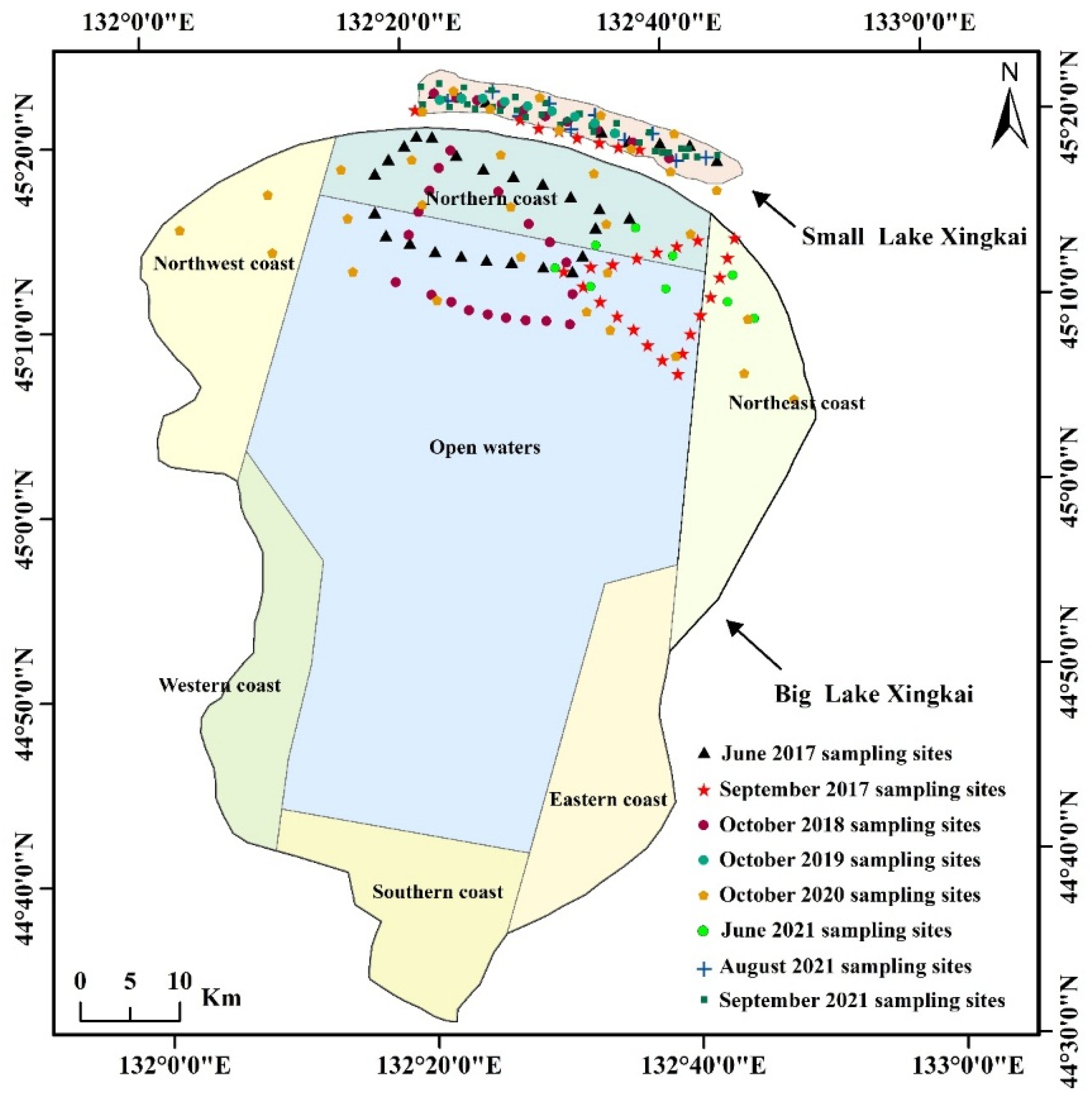
Lake Xingkai (44°32″–45°21″N, 131°58″–132°51″E), located on the border between China and Russia, is the largest freshwater lake in Northeast Asia [25] and covers an area of 4380 km² (Figure 1). A natural sand bar separates Lake Xingkai into two parts: Small Lake Xingkai and Big Lake Xingkai. The former is wholly located in China. The latter is located across the China–Russia border and most of its water is in Russia. The lake basin has a temperate continental monsoon climate, with less spring and autumn precipitation, more summer, and a long dry winter. The lake freezes in December and thaws in late April of the subsequent year [26]. It is fed by 26 rivers (9 in China and 17 in Russia) and has only one outflowing river in the northeast, the Songacha River, which flows into the Ussuri River [27]. For China and Russia, Lake Xingkai represents an essential food supply base and has tremendous economic and social value for flood control, irrigation, agriculture, and tourism, and plays a particular ecological function in regulating climate and improving water quality. Research on its water quality can provide data support for local environmental management and sustainable development. In this study, Big Lake Xingkai was divided into seven sub-regions, including the Northeast Coast, North Coast, Northwest Coast, West Coast, Open Waters, South Coast, and East Coast (Figure 1).

2.2. Field Sampling and Laboratory Analysis

Over the course of eight field experiments on Lake Xingkai, 260 samples were collected between 2017 and 2021 (Figure 1). Surface water (depth ~30 cm) was collected using a standard two-liter polyethylene water-sampling instrument and then transferred to cold, dark coolers in the laboratory for analysis within 24 h. The absorption coefficient of a total particular matter, subsequently separated into phytoplankton ($a_{ph}\left(\lambda \right)$) and detrital components ($a_d\left(\lambda \right)$) through bleaching with 80% hot ethanol, was measured following the quantitative filter technique approach [28]. The absorption coefficient of the dissolved organic matter ($a_g\left(\lambda \right)$) was determined spectrophotometrically with reference to ultrapure water using filtration of the water sample over a 0.2 μm membrane filter [28]. The sum of $a_d\left(\lambda \right)$ and $a_g\left(\lambda \right)$ was denoted as $a_{dg}\left(\lambda \right)$. The suspended particulate matter concentrations (SPM) were gravimetrically determined from samples that were dried at 105 °C overnight. SPM was differentiated into suspended particular inorganic matter and suspended particular organic matter by burning the organic matter from the filters at 450 °C for four hours [29]. The Chla concentrations were filtered on Whatman GF/F fiberglass filters and extracted with ethanol (80%) at 80 °C. The Chla concentration was determined spectrophotometrically [30].

The measurements were taken in Lake Xingkai for the samples collected between the local hours of 8:00 and 15:00 using a FieldSpec spectroradiometer (Analytical Spectral Devices, Inc.). The radiance of the water surface, sky, and a 30% gray board was measured over the ship’s deck. The $R_{rs}\left(\lambda \right)$ were extracted using the following Equation:

$$R_{rs}\left(\lambda \right)=\frac{(L_{sw}-r{L}_{sky}){\rho }_p}{L_p\pi }$$

(1)

2.3. Meteorological Data

Daily wind speed (m/s) and temperature (°C) in August of each year between 2016 and 2021 were downloaded from the Jixi meteorological station near Lake Xingkai.

2.4. Candidate Chla Algorithms for Lake Xingkai

Six proposed Chla algorithms, the two-band ratio method (BR), the three-band algorithm (TBA), a four-band algorithm (FBA), which is a simplified expression of the TC2 algorithm [17], the Fluorescence Line Height algorithm (FLH), the MERIS Maximum Chlorophyll Index (MCI), and the maximum peak-height (MPH) algorithm [31] were evaluated in Lake Xingkai. In the model construction of turbid inland waters, one of the most important steps was the extraction of $a_{ph}\left(\lambda \right)$ from $a_{nw}\left(\lambda \right)$ (removing $a_{dg}\left(\lambda \right)$). In the model assumption, the BR method ignored the ($a_{dg}\left(665\right)$, TBA considered $a_{dg}\left(709\right)$ nearly close to $a_{dg}\left(665\right)$, FBA thought of $a_{dg}\left(665\right)$ was approximately equal to ${0.17a}_{dg}\left(560\right)+0.83a_{dg}\left(709\right)$. FLH, MCI, and MPH attempt to remove $a_{dg}\left(\lambda \right)$ using baseline methods. The calculation steps of these algorithms were as follows:

$$BR=R_{rs}\left(709\right)/R_{rs}\left(665\right)$$

(2)

$$TBA={(1/R}_{rs}\left(665\right)-1/R_{rs}\left(709\right))\ast R_{rs}\left(754\right)$$

(3)

$$FBA={(1/R}_{rs}\left(665\right)-\frac{0.17}{R_{rs}\left(560\right)}-\frac{0.83}{R_{rs}\left(709\right)})\ast R_{rs}\left(754\right)$$

(4)

$$FLH=R_{rs}\left(681\right)-R_{rs}\left(665\right)-\left(R_{rs}\left(709\right)-R_{rs}\left(665\right)\right)\ast \frac{681-665}{709-665}$$

(5)

$$MCI=R_{rs}\left(709\right)-R_{rs}\left(665\right)-\left(R_{rs}\left(754\right)-R_{rs}\left(665\right)\right)\ast \frac{709-665}{754-665}$$

(6)

$$MPH=R_{rs}\left({\lambda }_{max}\right)-R_{rs}\left(665\right)-(R_{rs}\left(885\right)-R_{rs}\left(665\right))\ast ({\lambda }_{max}-665)/(885-665)$$

(7)

In Equation (7), $R_{rs}\left({\lambda }_{max}\right)$ and ${\lambda }_{max}$ are, respectively, the magnitude and position of the highest $R_{rs}\left({\lambda }_{max}\right)$ value from OLCI bands at 681, 709, and 754 nm.

2.5. Atmospheric Correction of OLCI Imagery

In this study, the process of atmospheric correction of OLCI imagery (denoted as Rud) was as follows.

The OLCI cloud-free subset radiance images in Lake Xingkai from May to October between 2016 and 2022 were downloaded from NASA’s Ocean Biology Processing Group (OBPG) (https://oceancolor.gsfc.nasa.gov/, 1 January 2020.).

In the first step, the Rayleigh corrected reflectance (${\mathrm{R}}_{\mathrm{r}\mathrm{c}}\left(\mathsf{\lambda }\right)$) was calculated with the SeaDAS package (version 8.2.0) OLCI products with Equation (8):

$$R_{rc}\left(\lambda \right)={\pi /F_0\left(\lambda \right)/cos\theta \ast (L}_t\left(\lambda \right)/t_{g_{sol}}\left(\lambda \right)/t_{g_{sen}}\left(\lambda \right)-L_r\left(\lambda \right)-{TL}_g\left(\lambda \right))$$

(8)

where $L_t\left(\lambda \right)$ represents the top-of-atmosphere (TOA) radiance, $L_r\left(\lambda \right)$ represents the Rayleigh radiance, ${TL}_g\left(\lambda \right)$ represents the TOA glint radiance, $\theta$ represents the solar zenith angle, $F_0\left(\lambda \right)$ represents the mean solar flux, $t_{g_{sol}}\left(\lambda \right)$ represents gaseous transmittance from the sun to the surface, and $t_{g_{sen}}\left(\lambda \right)$ represents gaseous transmittance from surface to sun.

The second step was the extraction of the lake water region. The lake boundary was obtained using one cloud-free OLCI image observed on 10 September 2018, considering this lake’s minimal water level variations. The lake boundary shapefile was drawn on a standard false color display by visual interpretation using ArcGIS 10.2. Then, the shapefile was converted to a raster image. A two-pixel buffer inward of the water boundary was removed to avoid the influence of adjacent land and substrates on nearby offshore water pixels.

The third step was obtaining the OLCI retrieved products. A near-infrared (NIR) bright pixel atmospheric correction was used in this study. The shape model in NIR bands proposed by Ruddick [32] was used to parametrize (Equation (9)).

$$R_{rs}\left(\lambda \right)=R_{rs}\left({\lambda }_0\right)\ast \frac{a_w\left({\lambda }_0\right)}{a_w\left(\lambda \right)}\ast {\left(\frac{\lambda }{{\lambda }_0}\right)}^{-\eta }$$

(9)

The reference band was 754 nm, and the parameterized bands were 779, 865, 885, and 1012 nm. The $a_w$ represents the absorption by pure water obtained from the OLCI “msl12_sensor_info.dat” in SeaDAS 8.0.2 (ocssw/share/olci, Table S1 in Supplementary Materials). Applying Equation (9) to Equation (8), the simulated $R_{rc}\left(\lambda \right)$ can be expressed as (denoted as $R_{rc}^{\ast }(\lambda )$):

$$R_{rc}^{\ast }(\lambda )=\frac{{\rho }_a\ast t\left({\lambda }_0\right)-{\rho }_a\ast t\left(\lambda \right)\ast \frac{a_w\left({\lambda }_0\right)}{a_w\left(\lambda \right)}\ast {\left(\frac{\lambda }{{\lambda }_0}\right)}^{-\eta }+R_{rc}({\lambda }_0)\ast t\left(\lambda \right)\ast \frac{a_w\left({\lambda }_0\right)}{a_w\left(\lambda \right)}\ast {\left(\frac{\lambda }{{\lambda }_0}\right)}^{-\eta }}{t\left({\lambda }_0\right)}$$

(10)

where $\eta$ represents a shape parameter that depends on the size of the particles, and ${\rho }_a$ represents the aerosol reflectance. In this study, the aerosol was assumed to be “white” (i.e., the aerosol reflectance was assumed to be wave-independent). The total diffuse atmosphere transmittance $t\left(\lambda \right)$ was calculated using the solar zenith angle ($\theta$), the satellite zenith angle (${\theta }_v$), the Rayleigh optical thickness (${\tau }_r(\lambda$)) and the ozone optical thickness (${\tau }_{O_z}(\lambda$)) [33] as:

$$t\left(\lambda \right)=exp\left(\right(-\frac{{\tau }_r\left(\lambda \right)}{2}+{\tau }_{O_z}\left(\lambda \right))/\mathit{cos}\theta )\ast exp\left(\right(-\frac{{\tau }_r\left(\lambda \right)}{2}+{\tau }_{O_z}\left(\lambda \right))/\mathit{cos}{\theta }_v)$$

(11)

The ${\tau }_r\left(\lambda \right)$ of each OLCI band in the standard atmospheric pressure (1013.25 hPa, denoted as ${\tau }_r^s\left(\lambda \right)$) was obtained from the OLCI Rayleigh lookup table in SeaDAS 8.2.0 (ocssw/share/olci). For each pixel in one specific OLCI image over Lake Xingkai, the ${\tau }_r\left(\lambda \right)$ was calculated as:

$${\tau }_r\left(\lambda \right)={\tau }_r^s\left(\lambda \right)\ast a_p/1013.25$$

(12)

where ${\mathrm{a}}_{\mathrm{p}}$ represents the National Centers for Environmental Prediction (NCEP) atmospheric pressure product in hPa obtained from the l2 gen process of SeaDAS 8.2.0. The ${\tau }_{O_z}\left(\lambda \right)$ was calculated by multiplying the ozone concentration (Ozone) in cm obtained from the SeaDAS l2 gen process by the ozone absorption coefficients (OAC) in matm-1$\ast$cm⁻¹ (Table S2 in the Supplementary Materials [34]):

$${\tau }_{O_z}\left(\lambda \right)=ozone\ast OAC$$

(13)

The fourth step was the identification of ${\rho }_a$. For each OLCI water pixel, the value of ${\rho }_a$ was set between 0 and the maximum of $R_{rc}\left(NIR\right)$ of this pixel ($R_{rc}^{max}\left(NIR\right)$) with a step of $R_{rc}^{max}\left(NIR\right)$/100; the value of $\mathsf{\eta }$ was set between −4 and +4 with a step of 0.1. For each combination of ${\mathsf{\rho }}_a$ and $\mathsf{\eta }$, we can obtain a group of $R_{rc}^{\ast }\left(NIR\right)$ at 779, 865, and 885 nm. The identification of ${\mathsf{\rho }}_a$ was done with the minimum Euclidean distance (MED) between $R_{rc}^{\ast }\left(NIR\right)$ and $R_{rc}\left(NIR\right)$:

$$\mathrm{M}\mathrm{E}\mathrm{D}=\sqrt{{(R_{rc}^{\ast }\left(779\right)-R_{rc}\left(779\right))}^2+{(R_{rc}^{\ast }\left(865\right)-R_{rc}\left(865\right))}^2+{(R_{rc}^{\ast }\left(885\right)-R_{rc}\left(885\right))}^2+{(R_{rc}^{\ast }\left(1012\right)-R_{rc}\left(1012\right))}^2}$$

(14)

The fifth step was the retrieval of $R_{rs}\left(\lambda \right)$. Applying the determined ${\rho }_a$ from Equation (14) and $t\left(\lambda \right)$ estimated from Equation (11), the $R_{rs}\left(\lambda \right)$ of each band of the OLCI water pixels were obtained with Equation (15):

$$R_{rs}\left(\lambda \right)={(R}_{rc}\left(\lambda \right)-{\rho }_a)/t\left(\lambda \right)/\pi$$

(15)

2.6. OLCI $R_{rs}\left(\lambda \right)$ Quality Control in Lake Xingkai

The valid OLCI $R_{rs}\left(\lambda \right)$ pixels were determined to be barely affected by clouds, cloud shadows, adjacency effects, sun glint, and higher sun zenith angle or viewing zenith angle. Here, we removed the invalid OLCI $R_{rs}\left(\lambda \right)$ pixels as follows.

The first step was masking thick clouds. The pixels that simultaneously satisfied $R_{rc}\left(412\right)>0.25$, $R_{rc}\left(442\right)>0.25$, and $R_{rc}\left(490\right)>0.25$ were regarded as thick cloud pixels and eliminated.

The second step was masking high solar zenith angles (Solz) or satellite zenith angles (Senz). In this study, strict high-angle limitations were used, and pixels were removed if Solz > 55° or Senz > 55°.

The third step was removing non-water pixels by the normalized difference water index (NDWI) calculated with Equation (16). By visual interpretation, the NDWI of the water pixels covered by thin clouds or submerged aquatic vegetation, influenced by the adjacency efforts, often was <0.3. With the threshold of NDWI $\ge$ 0.3, we can remove most of these non-water pixels.

$$\mathrm{N}\mathrm{D}\mathrm{W}\mathrm{I}=\left(R_{rc}\right(560)-R_{rc}(1012\left)\right)/(R_{rc}\left(560\right)+R_{rc}(1012\left)\right)$$

(16)

The fourth step was the removal of non-water pixels by visual inspection. Water pixels were eliminated in the following situations: (1) submerged aquatic vegetation influenced the water pixels, and (2) undetected clouds or cloud shadows still covered the water pixels.

2.7. Production of Matchups (Synchronous Satellite $R_{rs}\left(\lambda \right)$ and In Situ Chla) for Chla Model Development

The time window between the valid OLCI $R_{rs}\left(\lambda \right)$ and in situ samples was set as <1 day. If the number of the valid OLCI $R_{rs}\left(\lambda \right)$ pixels within a 3 × 3 window centered at the location of each in situ sample was nine, and the coefficient of variation (CV) of the valid spectra was <0.15, the median $R_{rs}\left(\lambda \right)$ of these valid pixels was calculated as the OLCI $R_{rs}\left(\lambda \right)$ of this sample. Based on these criteria, a total of 119 matchups (synchronous OLCI $R_{rs}\left(\lambda \right)$ and in situ Chla) were selected. We evenly divided the matchup data into two parts: one part of 60 samples was used to calibrate the candidate models for estimating Chla from OLCI image data, and the other part comprising 59 samples, was used to validate these models.

2.8. Accuracy Assessment

We used five evaluation indicators to evaluate the accuracy of these Chla models, including coefficient of determination (R²), relative difference (RD), mean normalized difference (MND), mean absolute percentage difference (MAPD), and root-mean-square deviation (RMSD):

$${\mathrm{R}}^2=\frac{\sum _{\mathrm{i}=1}^{\mathrm{N}}{({\mathrm{V}\mathrm{a}\mathrm{l}\mathrm{u}\mathrm{e}}_{\mathrm{p}\mathrm{r}\mathrm{e}\mathrm{d}\mathrm{i}\mathrm{c}\mathrm{t}\mathrm{e}\mathrm{d},\mathrm{i}}-\overline{{\mathrm{V}\mathrm{a}\mathrm{l}\mathrm{u}\mathrm{e}}_{\mathrm{m}\mathrm{e}\mathrm{a}\mathrm{s}\mathrm{u}\mathrm{r}\mathrm{e}\mathrm{d}}})}^2}{\sum _{\mathrm{i}=1}^{\mathrm{N}}{({\mathrm{V}\mathrm{a}\mathrm{l}\mathrm{u}\mathrm{e}}_{\mathrm{m}\mathrm{e}\mathrm{a}\mathrm{s}\mathrm{u}\mathrm{r}\mathrm{e}\mathrm{d},\mathrm{i}}-\overline{{\mathrm{V}\mathrm{a}\mathrm{l}\mathrm{u}\mathrm{e}}_{\mathrm{m}\mathrm{e}\mathrm{a}\mathrm{s}\mathrm{u}\mathrm{r}\mathrm{e}\mathrm{d}}})}^2}$$

(17)

$$\mathrm{R}\mathrm{D}=\left|\frac{{\mathrm{V}\mathrm{a}\mathrm{l}\mathrm{u}\mathrm{e}}_{\mathrm{m}\mathrm{e}\mathrm{a}\mathrm{s}\mathrm{u}\mathrm{r}\mathrm{e}\mathrm{d},\mathrm{i}}-{\mathrm{V}\mathrm{a}\mathrm{l}\mathrm{u}\mathrm{e}}_{\mathrm{p}\mathrm{r}\mathrm{e}\mathrm{d}\mathrm{i}\mathrm{c}\mathrm{t}\mathrm{e}\mathrm{d},\mathrm{i}}}{{\mathrm{V}\mathrm{a}\mathrm{l}\mathrm{u}\mathrm{e}}_{\mathrm{m}\mathrm{e}\mathrm{a}\mathrm{s}\mathrm{u}\mathrm{r}\mathrm{e}\mathrm{d},\mathrm{i}}}\right|\ast 100\mathrm{\%}$$

(18)

$$\mathrm{M}\mathrm{N}\mathrm{D}=\frac{1}{\mathrm{N}}{\sum }_{\mathrm{i}=1}^{\mathrm{N}}\frac{{\mathrm{V}\mathrm{a}\mathrm{l}\mathrm{u}\mathrm{e}}_{\mathrm{m}\mathrm{e}\mathrm{a}\mathrm{s}\mathrm{u}\mathrm{r}\mathrm{e}\mathrm{d},\mathrm{i}}-{\mathrm{V}\mathrm{a}\mathrm{l}\mathrm{u}\mathrm{e}}_{\mathrm{p}\mathrm{r}\mathrm{e}\mathrm{d}\mathrm{i}\mathrm{c}\mathrm{t}\mathrm{e}\mathrm{d},\mathrm{i}}}{{\mathrm{V}\mathrm{a}\mathrm{l}\mathrm{u}\mathrm{e}}_{\mathrm{m}\mathrm{e}\mathrm{a}\mathrm{s}\mathrm{u}\mathrm{r}\mathrm{e}\mathrm{d},\mathrm{i}}}\ast 100\mathrm{\%}$$

(19)

$$\mathrm{M}\mathrm{A}\mathrm{P}\mathrm{D}=\frac{1}{\mathrm{N}}{\sum }_{\mathrm{i}=1}^{\mathrm{N}}\left|\frac{{\mathrm{V}\mathrm{a}\mathrm{l}\mathrm{u}\mathrm{e}}_{\mathrm{m}\mathrm{e}\mathrm{a}\mathrm{s}\mathrm{u}\mathrm{r}\mathrm{e}\mathrm{d},\mathrm{i}}-{\mathrm{V}\mathrm{a}\mathrm{l}\mathrm{u}\mathrm{e}}_{\mathrm{p}\mathrm{r}\mathrm{e}\mathrm{d}\mathrm{i}\mathrm{c}\mathrm{t}\mathrm{e}\mathrm{d},\mathrm{i}}}{{\mathrm{V}\mathrm{a}\mathrm{l}\mathrm{u}\mathrm{e}}_{\mathrm{m}\mathrm{e}\mathrm{a}\mathrm{s}\mathrm{u}\mathrm{r}\mathrm{e}\mathrm{d},\mathrm{i}}}\right|\ast 100\mathrm{\%}$$

(20)

$$\mathrm{R}\mathrm{M}\mathrm{S}\mathrm{D}=\sqrt{\frac{{\sum }_{\mathrm{i}=1}^{\mathrm{N}}{({\mathrm{V}\mathrm{a}\mathrm{l}\mathrm{u}\mathrm{e}}_{\mathrm{m}\mathrm{e}\mathrm{a}\mathrm{s}\mathrm{u}\mathrm{r}\mathrm{e}\mathrm{d},\mathrm{i}}-{\mathrm{V}\mathrm{a}\mathrm{l}\mathrm{u}\mathrm{e}}_{\mathrm{p}\mathrm{r}\mathrm{e}\mathrm{d}\mathrm{i}\mathrm{c}\mathrm{t}\mathrm{e}\mathrm{d},\mathrm{i}})}^2}{\mathrm{N}}}$$

(21)

where ${\mathrm{V}\mathrm{a}\mathrm{l}\mathrm{u}\mathrm{e}}_{\mathrm{m}\mathrm{e}\mathrm{a}\mathrm{s}\mathrm{u}\mathrm{r}\mathrm{e}\mathrm{d},\mathrm{i}}$ is the reference value from the in situ measurements, ${\mathrm{V}\mathrm{a}\mathrm{l}\mathrm{u}\mathrm{e}}_{\mathrm{p}\mathrm{r}\mathrm{e}\mathrm{d}\mathrm{i}\mathrm{c}\mathrm{t}\mathrm{e}\mathrm{d},\mathrm{i}}$ represents the value derived by the algorithms; $\overline{{\mathrm{V}\mathrm{a}\mathrm{l}\mathrm{u}\mathrm{e}}_{\mathrm{m}\mathrm{e}\mathrm{a}\mathrm{s}\mathrm{u}\mathrm{r}\mathrm{e}\mathrm{d}}}$ is the mean value of all the ${\mathrm{V}\mathrm{a}\mathrm{l}\mathrm{u}\mathrm{e}}_{\mathrm{p}\mathrm{r}\mathrm{e}\mathrm{d}\mathrm{i}\mathrm{c}\mathrm{t}\mathrm{e}\mathrm{d},\mathrm{i}}$, and N is the number of observations.

3. Results

3.1. Calibration and Validation of Chla Algorithms

In this study, the atmospheric correction performance of Rud was validated using the synchronous in situ $R_{rs}\left(\lambda \right)$ (Figures S8 and S9, and Table S3). For the bands, including the 665, 681, 709, 754, and 885 nm that were used for the Chla algorithms, the mean MAPDs, MNDs, and RMSDs were 16.44%, −6.8%, and 0.0052 sr⁻¹, respectively. Rud outperformed the commonly used C2RCC algorithm in Lake Xingkai. Thus, Rud was used to produce the long-time series OLCI $R_{rs}\left(\lambda \right)$ products in this Lake. The calibration dataset with in situ Chla concentrations ranging from 0.4 to 13.59 mg m⁻³ was used to establish the expression of the BR, TBA, MCI, FLH, MPH, and FBA algorithms (Figure 2, Equations (2)–(7)). Different regression methods (exponential, linear, logarithmic, second-order polynomial, and power) were tested, and the method with the highest R² was selected for each algorithm as follows:

y = 51.152 × BR² − 35.672 × BR − 4.9263

(22)

y = 143.12 × TBA² + 117.45 × TBA + 10.375

(23)

y = 371998 × MCI² − 2976.2 × MCI + 10.568

(24)

y = −42853 × FLH² − 3608.6 × FLH + 6.5238

(25)

y = 960594 × MPH² − 3585.9 × MPH + 7.5487

(26)

y = 507.02 × FBA² + 169.7 × FBA + 10.313

(27)

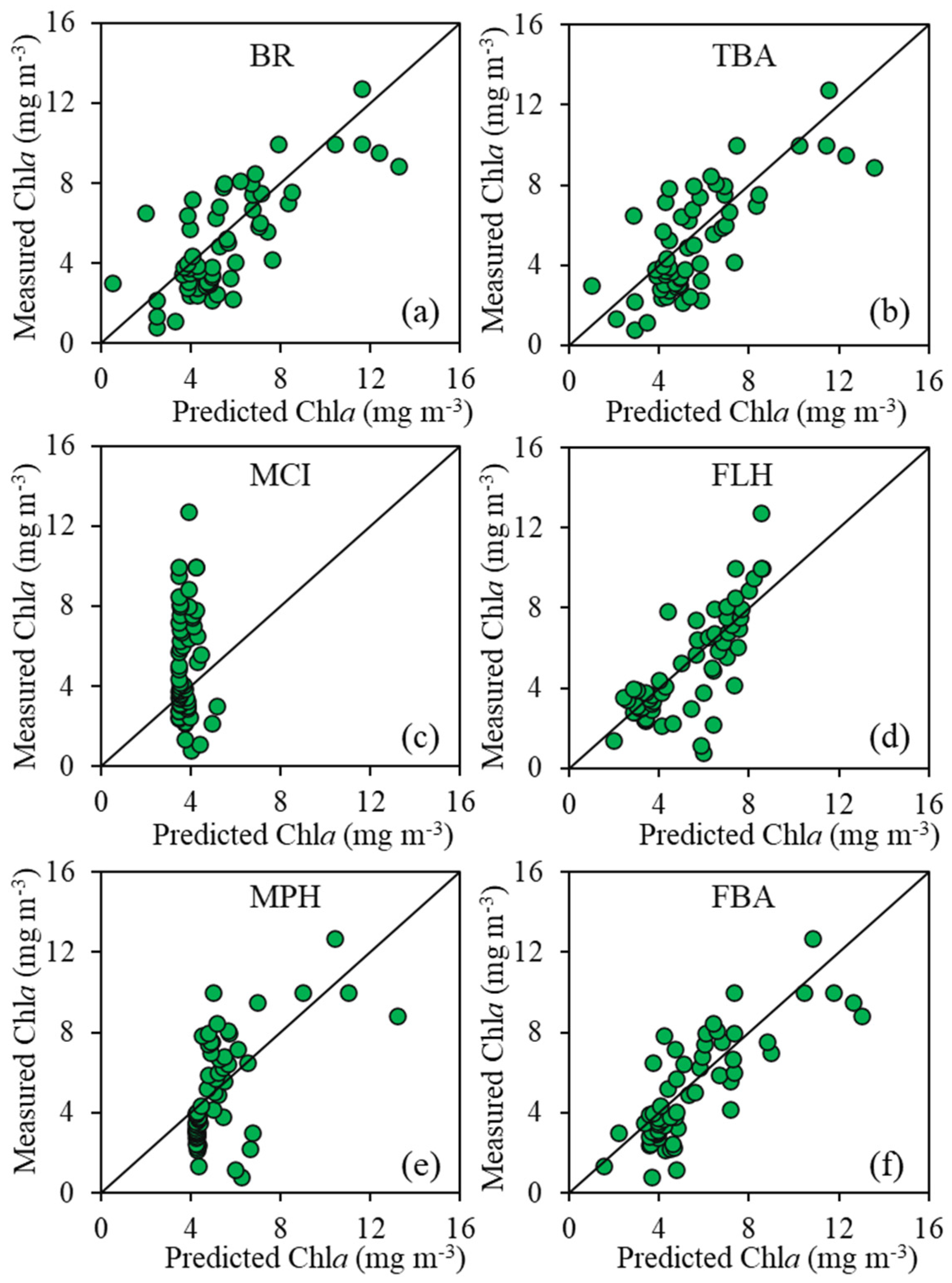
For each algorithm, a second-order polynomial regression function had the highest R² compared with other regression function types. Previous studies [35,36,37] agreed that a second-order polynomial regression function is a good choice in the construction of water-quality parameters retrieving models for turbid waters with algae (case-II waters). Thus, all these models were calibrated using the second-order polynomial regression type. Figure 3 shows strong and similar relationships between each reflectance index of BR, TBA, and FBA (R² = 0.64, 0.58, and 0.67, respectively). The relationships between the reflectance indices of MCI and MPH were weaker (R² = 0.04 and 0.25).

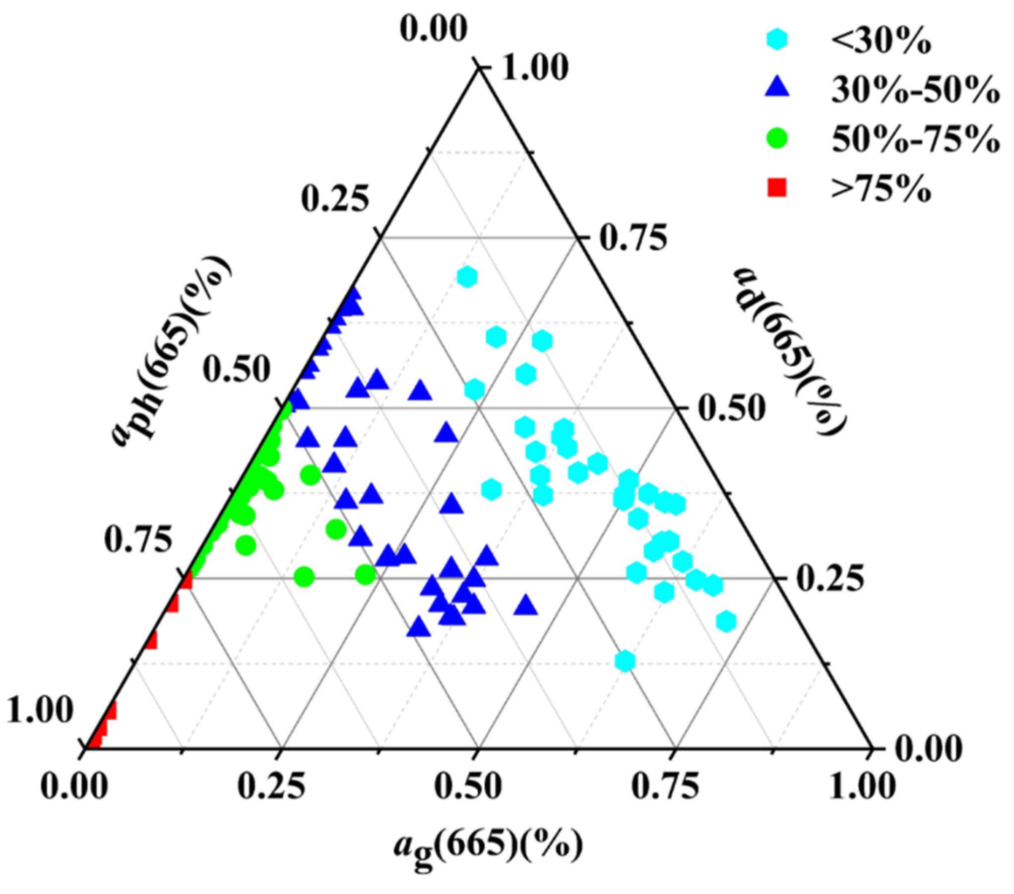
The performance of all the algorithms (Equations (22)–(27)) was validated using the validation dataset (Figure 3 and

Table 1. Performance of different algorithms in Lake Xingkai.

Algorithms	R2	MAPD (%)	MND (%)	RMSD (mg m−3)
BR	0.57	41.49	24.82	1.85
TBA	0.56	43.02	27.11	1.85
MCI	0	49.52	2.12	2.98
FLH	0.60	40.94	27.41	1.68
MPH	0.34	54.65	35.58	2.14
FBA	0.64	38.26	24.60	1.66

). A positive MND value indicates an overestimation of the Chla concentrations by these algorithms. Regarding R², FBA showed the best performance (R² = 0.64), and FLH, BR, and TBA followed closely (R² = 0.60, 0.57, and 0.56, respectively). The estimated Chla concentrations of MCI and MPH were weakly correlated with in situ Chla concentrations; thus, these algorithms were not used for the rest of the analysis. The MAPD and RMSD of the remaining four algorithms showed a similar performance to R². FBA had the lowest value (MAPD = 38.26% and RMSD = 1.66 mg m⁻³), and the other three algorithms followed (FLH: MAPD = 40.94%, and 1.68 mg m⁻³, BR: 41.49%, and 1.85 mg m⁻³, and TBA: 43.02%, and 1.85 mg m⁻³). The results indicated that FBA was the best-performing algorithm compared to the other five. We counted the contribution of $a_{\mathrm{p}\mathrm{h}}\left(\mathsf{\lambda }\right)$ to the total non-water absorption ($a_{\mathrm{n}\mathrm{w}}\left(\mathsf{\lambda }\right)$), the sum of $a_{\mathrm{p}\mathrm{h}}\left(\mathsf{\lambda }\right)$, $a_{\mathrm{g}}\left(\mathsf{\lambda }\right)$, and $a_{\mathrm{d}}\left(\mathsf{\lambda }\right)$) at 665 nm for the samples in Lake Xingkai (Figure 4). Although located near the phytoplankton peak, there were few samples in which the phytoplankton absorption was dominated. Thus, FBA, which had a reasonable assumption in removing $a_{\mathrm{g}}\left(665\right)$ and $a_{\mathrm{d}}\left(665\right),$ was selected as the algorithm to retrieve Chla concentrations in Lake Xingkai using OLCI images from June to October between 2016 and 2022.

3.2. Spatial and Temporal Variations of Chla Concentrations in Lake Xingkai

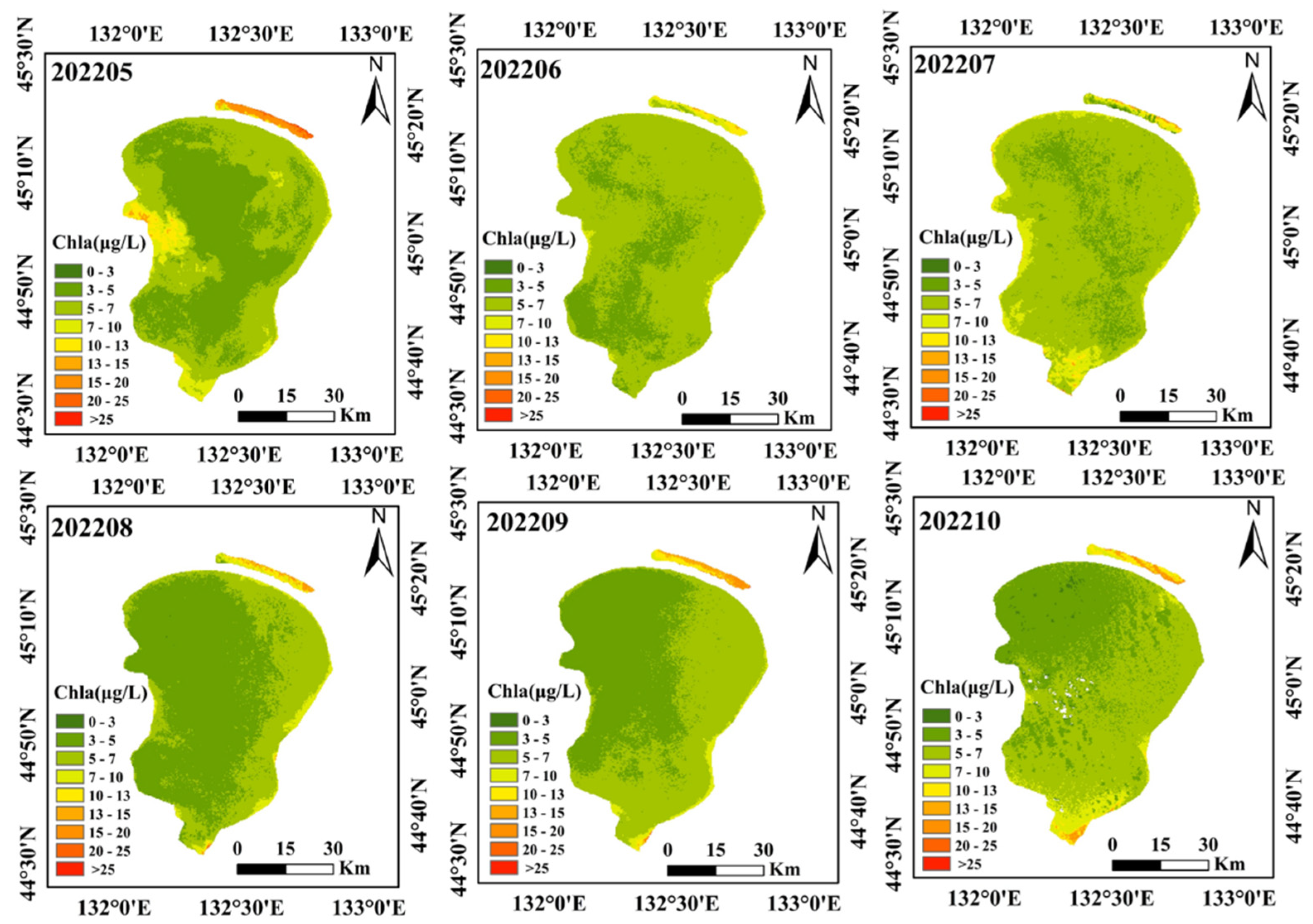
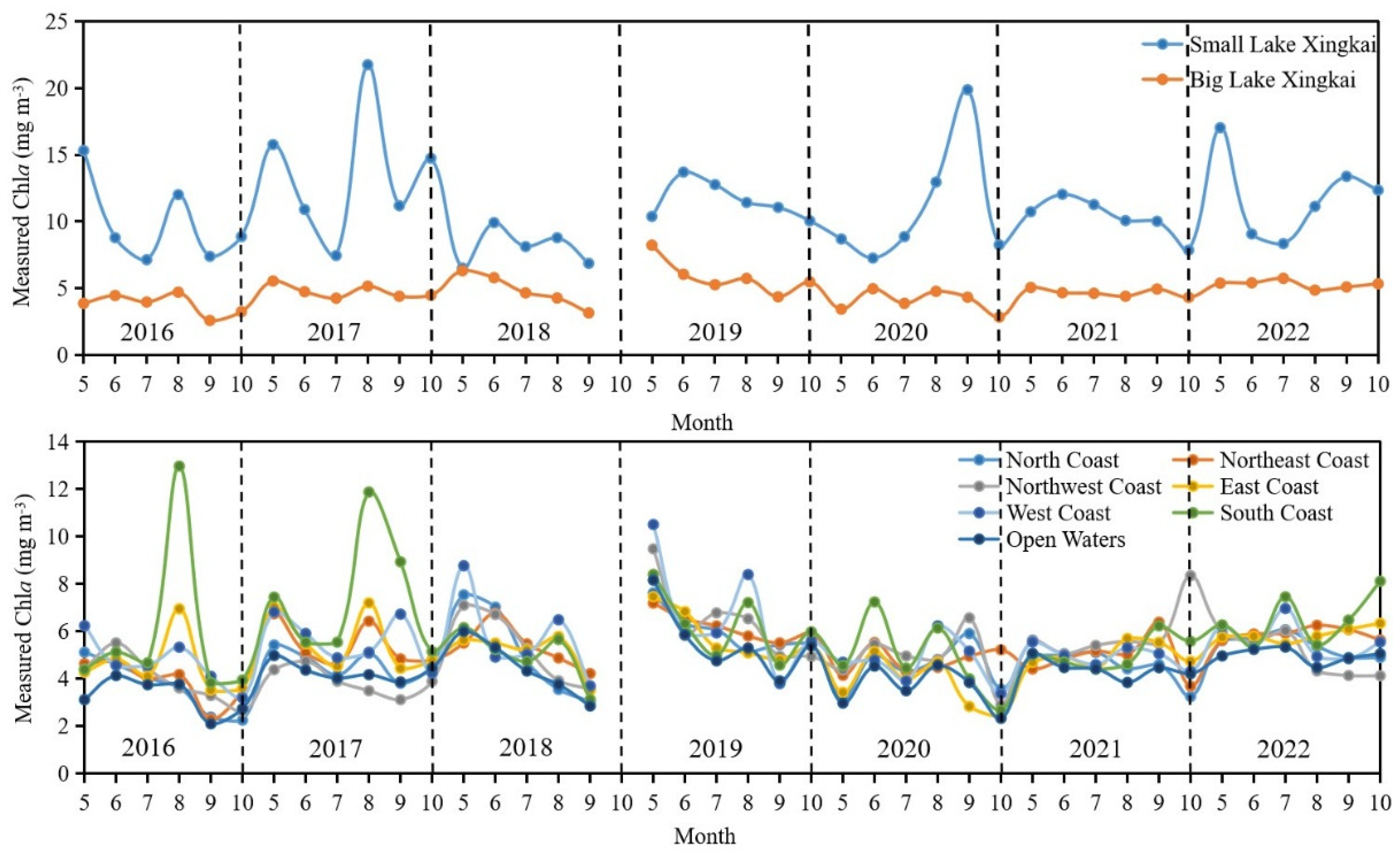
The OLCI-retrieved Chla products by the FBA algorithm from May to October between 2016 and 2022 were used to evaluate the phytoplankton biomass variation in this Lake (the monthly mean Chla maps in 2022 are shown in Figure 5, and 2016, 2017, 2018, 2019, 2020, and 2021 are shown in Figures S1–S6). Big Lake Xingkai and Small Lake Xingkai generally had relatively low Chla concentrations (with a long-term annual mean Chla concentration of 4.74 and 10.98 mg m⁻³) compared with other lakes with frequent blooms in China (e.g., Lake Taihu [1,38], Lake Chaohu [39], and Lake Dianchi [40]). The trophic status of Small Lake Xingkai was higher than that of Big Lake Xingkai. The maximum monthly mean value of Small Lake Xingkai (21.75 mg m⁻³) appeared in August 2017, while that of Big Lake Xingkai (8.23 mg m⁻³) appeared in May 2019. The minimum monthly mean value of Small Lake Xingkai (6.50 mg m⁻³) appeared in May 2018, and that of Big Lake Xingkai (2.56 mg m⁻³) appeared in September 2016. Overall, the Chla spatial difference of Big Lake Xingkai was not noticeable, except during specific months with relatively high values (August 2016 and August 2017) in the South Coast sub-region. The South Coast was the sub-region with the highest Chla concentrations, ranging from 2.67 mg m⁻³ in October 2020 to 12.97 mg m⁻³ in August 2016, with a long-term annual mean of 5.86 mg m⁻³. The Open Waters was the sub-region with the lowest Chla concentrations ranging from 2.09 mg m⁻³ in September 2016 to 8.16 mg m⁻³ in May 2019, with a long-term annual mean of 4.37 mg m⁻³. The long-term Chla annual mean of the rest of the sub-regions, North Coast, Northwest Coast, East Coast, Northeast Coast, and West Coast, were 4.84, 5.04, 5.09, 5.2, and 5.42 mg m⁻³, respectively.

Unlike other Chinese lakes with frequent algal blooms, which have relatively stable seasonal Chla variation patterns (e.g., Lake Taihu and Lake Chaohu often have relatively higher values in summer and autumn and relatively lower values in winter and spring) [41,42,43], the seasonal Chla variation trends in Lake Xingkai varied across years (Figure 6). The minimum (maximum) monthly mean Chla value in 2016, 2017, 2018, 2019, 2020, 2021, and 2022 were in July (May), July (August), May (June), October (June), June (September), October (June), July (May) in Small Lake Xingkai, and in September (August), July (May), September (May), September (May), October (June), October (May), and August (July) in Big Lake Xingkai.

4. Discussion

4.1. Reduction of Chla Model Accuracy Due to High Sun Angle

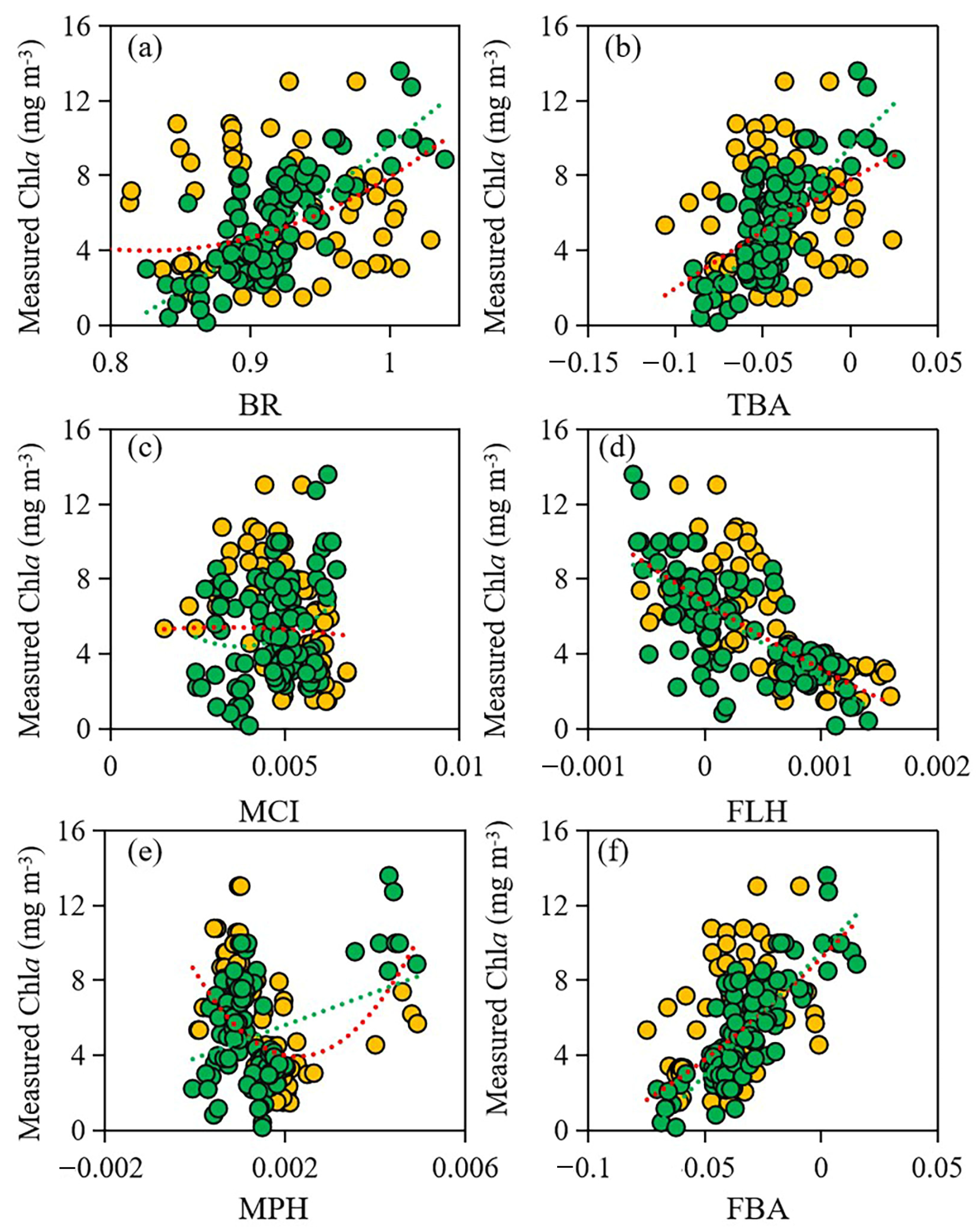
We only retained the sampling with both sun zenith angle (Solz) and satellite zenith angle (Senz) < 55° for model calibration and validation. The threshold was stricter than the one proposed by Bailey and Werdell [44] for NASA’s ocean watercolor products with Solz < 70° and Senz < 60°. This study selected a stricter Solz and Senz threshold because we found an observable decrease in the performance of atmospheric correction when Solz > 55° in Lake Xingkai. The correlation between in situ Chla concentrations and the spectral index of the well-performing models in Lake Xingkai decreased when only the data with Solz > 55° were added (Figure 7). The R² of FBA, TBA BR, and FLH decreased from 0.67, 0.58, 0.60, and 0.56 to 0.40, 0.23, 0.19, and 0.46, respectively.

Some studies have shown that a high Solz or Senz angle will increase the residual errors in satellite ${\mathrm{R}}_{\mathrm{r}\mathrm{s}}\left(\mathsf{\lambda }\right)$ products due to many factors, including higher atmospheric multiple scattering effects and underestimation of the Rayleigh contribution [44,45]. The atmospheric correction methods for waters originated from oceans and were then applied or improved to inland waters. The aerosol models in SeaDAS, the software package for processing ocean color data of NASA, were built based on analyzing aerosol properties of eight open seas and three coastal AERONET stations [46]. Aerosols over land often tend to have more absorbent particles and larger aerosol optical thickness than those over sea [47,48,49]. Using aerosol models designed for coastal waters and oceans to perform the atmospheric correction of inland waters may have uncertainties due to the different optical properties of aerosols between land and sea, especially when the Solz were high, like >55° as in Lake Xingkai.

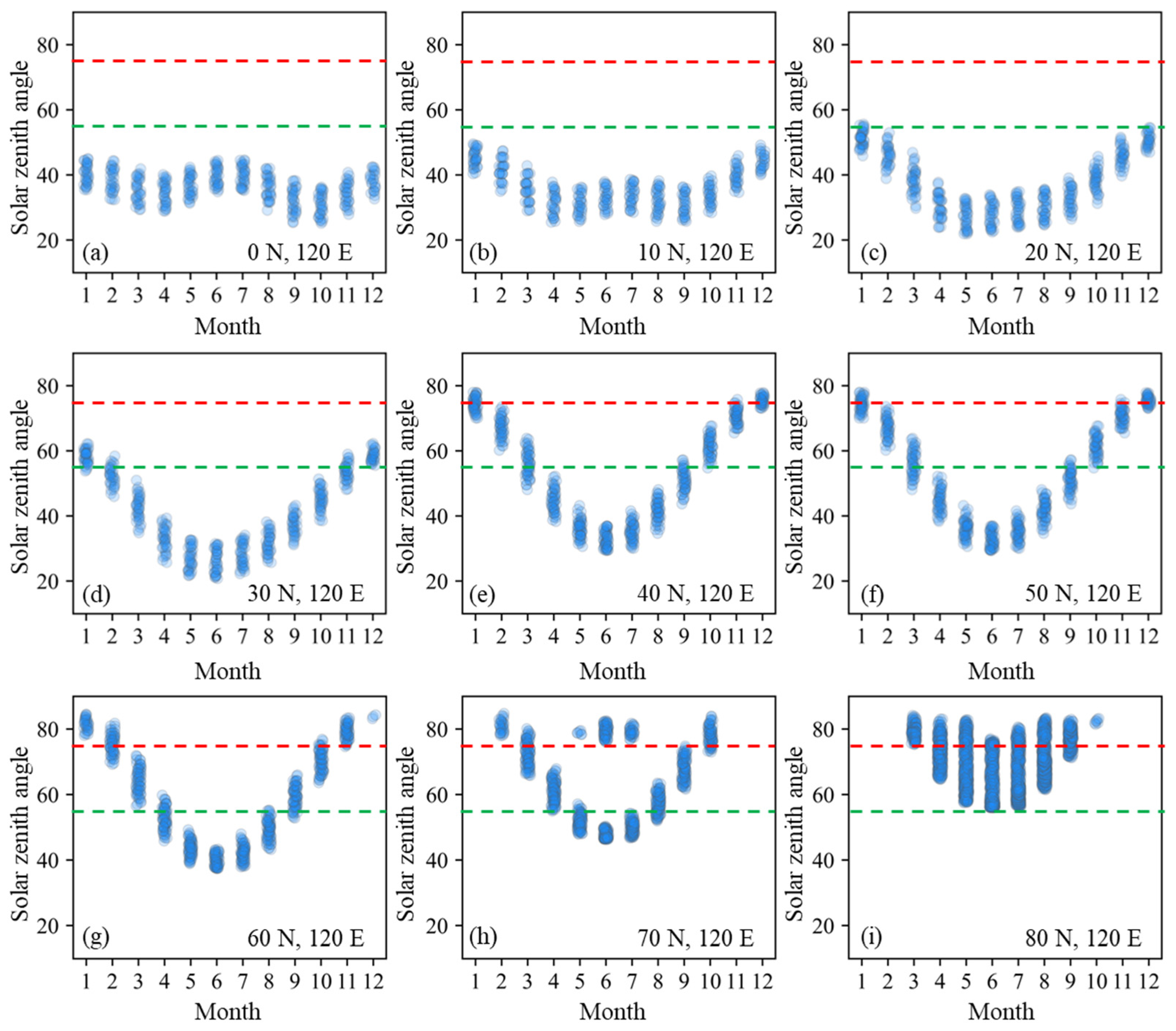
The OLCI ${\mathrm{R}}_{\mathrm{r}\mathrm{s}}\left(\mathsf{\lambda }\right)$ products of other inland lakes of the global middle and high latitudes also may use this strict threshold to ensure the ${\mathrm{R}}_{\mathrm{r}\mathrm{s}}\left(\mathsf{\lambda }\right)$ products with good quality, but it will reduce the number of valid OLCI images. In this study, we select five regions (the longitude and latitude ranges were 1°, with center latitude at 0°N, 10°N, 20°N, 30°N, 40°N, 50°N, 60°N, 70°N, 80°N and with the same longitude of 120°E) to analyze the OLCI solar observation differences over a whole year (2021). All the available OLCI images of these nine regions were downloaded and processed to obtain each image’s solar observation data for 2021. Without consideration of clouds, sunglint, ice, or other certifications, the solar observation information for different months is shown in Figure 8. The 0°N and 10°N regions did not have days with Solz > 55° for the entire year. The rate of high Solz angle images increased with latitude. At latitudes $\ge$ 40°N, most days in October and November (when many lakes are not yet frozen in the northern hemisphere) with Solz > 55° were not used to retrieve Chla concentrations, resulting in the absence of Chla inversion products this month. This indicates that in autumn, valid data of lakes located in the mid or high-latitude ranges may be less than those in the lower latitudes. For example, in October 2018, Lake Xingkai had seven scenes without clouds and obvious sunglint. However, because the Solz of all these images was >55°, they were not used to retrieve Chla concentrations, resulting in the absence of Chla inversion products in this month (Figure 5 and Figure S3). We also counted the Senz angle distribution at different months for regions at different latitudes (Figure S7). Unlike the Solz, Senz did not vary with latitude. The Senz of most images was <55°.

4.2. Limitations of Using Retrieved Chla Products to Evaluate the Trophic Status of the Lake

Unfortunately, the Chla product used in this study did not cover areas with dense algal blooms, which are the most intuitive manifestation of lake eutrophication. There are many reasons why previously proposed Chla algorithms or products are not suitable for algal blooms. Algae floating on the water’s surface have higher NIR reflectance than water. The assumptions of most atmospheric correction and Chla retrieval algorithms are, therefore, invalid in this situation. Additionally, the NDWI of dense algal blooms is often negative, and therefore, a positive NDWI threshold for extracting water pixels would also remove the algal bloom pixels [23,41]. The algal bloom area usually had large Chla concentrations, >10 mg m⁻³ [50,51], >100 mg m⁻³ [20], or even >1000 mg m⁻³ [52]. Masking the algal bloom area would underestimate the lake’s trophic status when using the retrieved Chla products (Figure 9). Thus, many studies used both the retrieved Chla concentrations and the extracted bloom areas to assess the trophic status of a lake [21,42]. It is not intuitive to use two indicators with different meanings. Many oligotrophic and mesotrophic lakes also have algal blooms [53,54]. Conversely, the waters classified as eutrophic (e.g., Chla > 10 mg m⁻³) by the trophic state index maybe not present algal blooms.

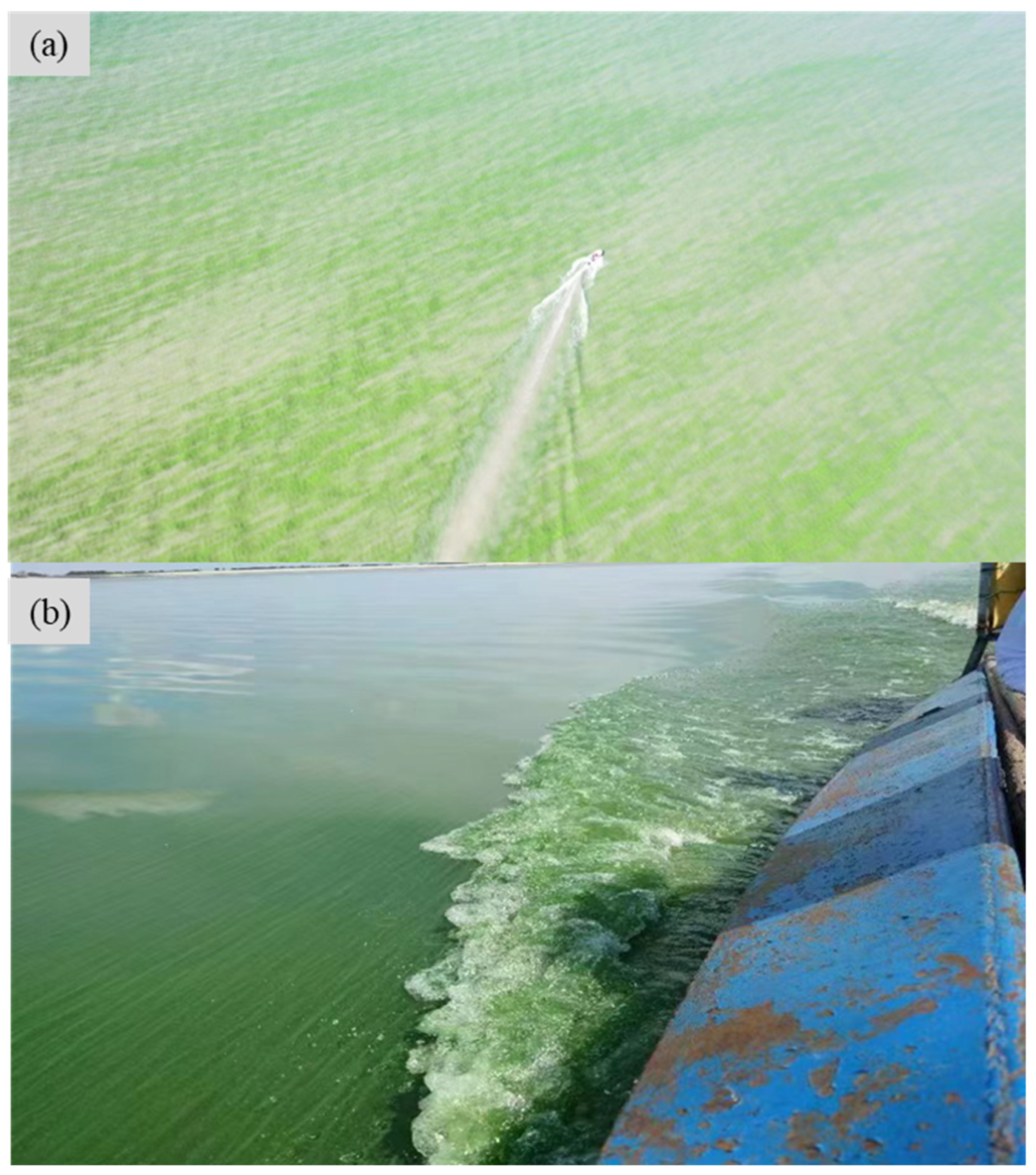
Only using satellite-retrieved Chla concentrations to measure the trophic status of water bodies will be clear. Few algorithms have been proposed for the Chla estimation of algal blooms. Many studies showed that the MPH algorithm performed well for algal blooms in some African lakes [31,55,56]. The relatively worse performance of MPH compared with FLH, BR, TBA, and FBA for waters with no algal bloom in Lake Xingkai indicated that we may need hybrid algorithms to retrieve Chla concentrations across blooming and non-blooming waters. It is vital to match synchronous satellite images with in situ samples when constructing atmospheric correction methods and Chla retrieval models for waters with algal blooms. Our experience indicated that obtaining accurate matches for blooming waters by ship is difficult. The waves caused by the boat will affect the algal bloom floating state during sampling (Figure 10). Additionally, the commonly used time window for inland lakes ($\le$3 h, $\le$1 day, or $\le$3 days) may be invalid. Therefore, we may need other data sampling methods, such as buoys, drones, and ground-based spectrometers, to collect samples for model calibration and validation.

4.3. Risk of Increased Trophic Status of Lake Xingkai Due to Increased Phytoplankton Biomass

In the past fifty years, the Lake Xingkai basin has become an important granary for China and Russia. Many wastelands, natural wetlands, woodlands, river beaches, etc., in the area have been reclaimed as farmland [57,58], creating a problem of agricultural non-point source pollution. The nutrient concentration in this lake is also very high. The measured total phosphorous of all our samples of Lake Xingkai was 0.112 mg L⁻¹, which is similar to those of other highly eutrophic lakes in China, have the following values: Lake Taihu (0.081 mg L⁻¹), Lake Chaohu (0.108 mg L⁻¹), and Lake Dianchi (TP 0.135 mg L⁻¹) [59]. Sufficient nutrients provide the primary conditions for the rapid growth of algae in Lake Xingkai.

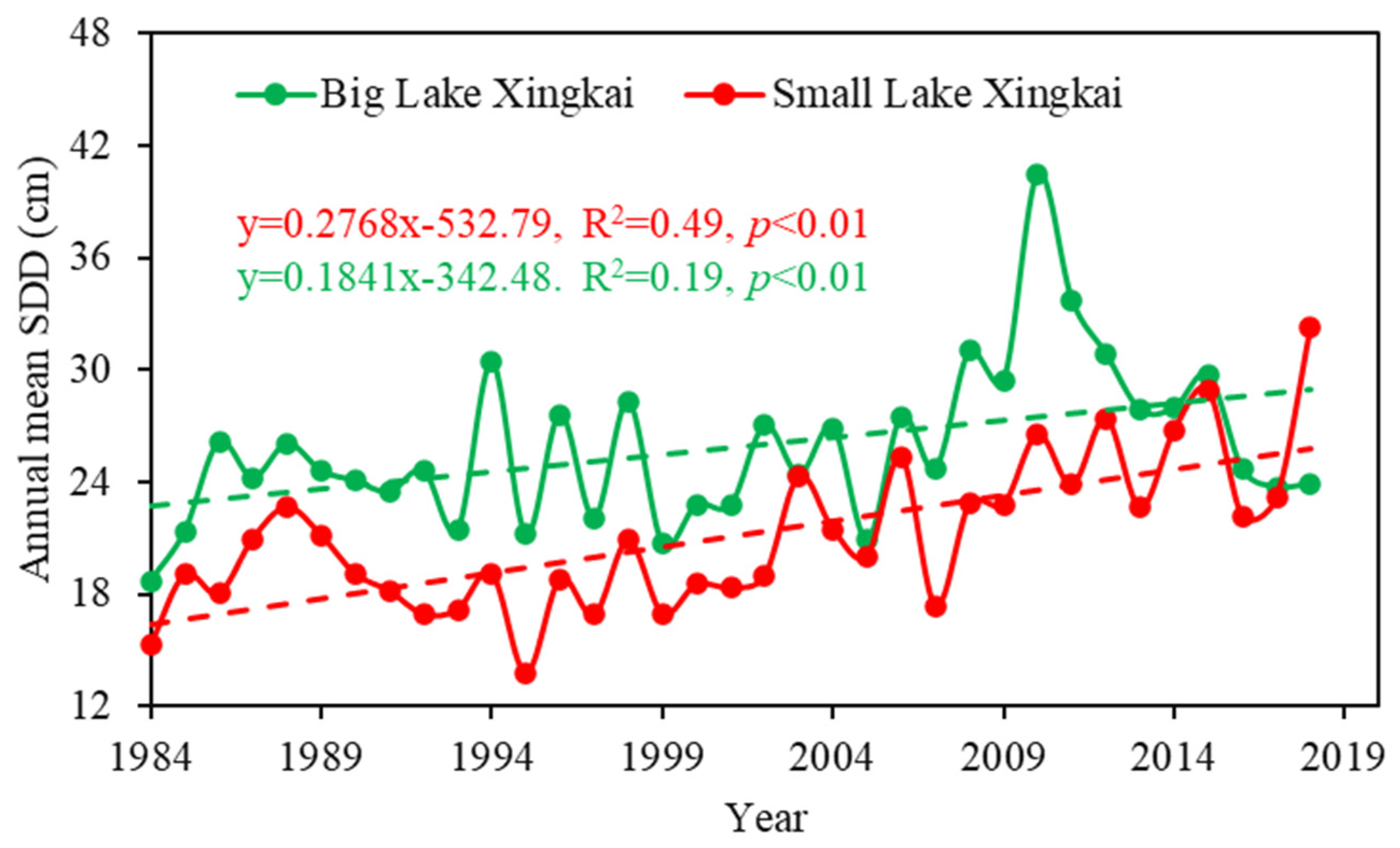
We also gauged the possible effects of increased water clarity and air temperature on the phytoplankton biomass of Lake Xingkai. The in situ Chla concentrations significantly correlated with the in situ measured SDD. It may be presumed that the change in water clarity may be a factor that affects the phytoplankton biomass in Lake Xingkai. Results from Lake Chagan, another turbid lake in the same region of Northeast China, showed that the total suspended matter (SPM, which had a high correlation with SDD in Lake Xingkai) is the main controlling factor limiting phytoplankton biomass [60]. The water clarity in Lake Xingkai has been increasing in the last few decades using long-time series of Landsat images (Figure 11) [61]. Between 1984 and 2018, the SDD of Small Lake Xingkai and Big Lake Xingkai showed an increasing trend, with a mean rate of 0.2728 and 0.1840 cm per year, respectively. Increased water clarity may result in more light entering the water and promote the growth of phytoplankton, increasing the risk of algal blooms in this lake.

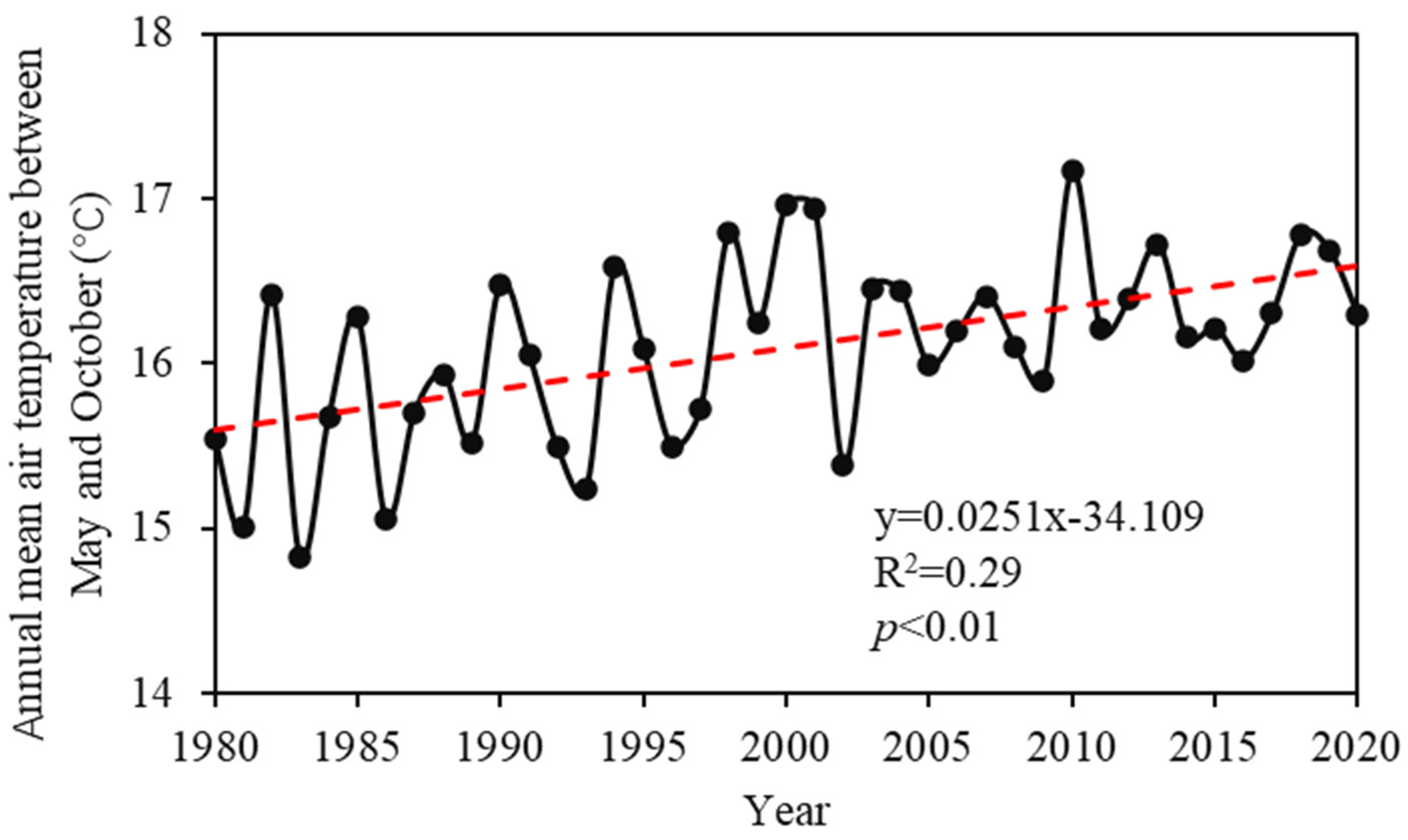
Northeast China has been one of the most rapidly warming regions of China and East Asia [62]. Figure 12 shows the annual average air temperature between May and October (the non-frozen period) observed at the Jixi meteorological station near Lake Xingkai from 1980 to 2020. In the past forty years, the annual average air temperature in the Jixi has shown an increasing trend, with a mean rate of 0.0251 °C per year. Like greater water clarity, warmer air temperatures also promote the growth of phytoplankton, increasing the trophic status of this lake.

5. Conclusions

In this study, we compared six Chla-retrieved models in Lake Xingkai, a typical turbid but rarely noticed mid-high latitude lake in Northeast Asia. The best-performed algorithm, the FBA algorithm, had a reasonable assumption in removing $a_{\mathrm{g}}\left(665\right)$ and $a_{\mathrm{d}}\left(665\right)$ was selected as the algorithm to retrieve Chla concentrations in Lake Xingkai using OLCI images from June to October between 2016 and 2022. Big Lake Xingkai and Small Lake Xingkai generally had relatively low Chla concentrations (with a long-term annual mean Chla concentration of 4.74 and 10.98 mg m⁻³).

We also gauged the uncertainties and limitations of using satellite images to monitor Chla concentrations of mid-high latitude lakes by taking Lake Xingkai as an example. We found a large decrease in accuracy when the Chla retrieval models were applied to the images with Solz > 55°. Meanwhile, we also gauged the limitations of remote-sensing Chla products for evaluating the trophic status of lakes due to the absence of areas with algal blooms. We suggest using hybrid algorithms to retrieve Chla concentrations across non-algal bloom and bloom waters.

We also found uncertainties and limitations of the Chla algorithm models when using a larger satellite zenith angle or applying it to an algal bloom area. Recent increases in anthropogenic nutrient loading, water clarity, and warming temperatures may lead to rising phytoplankton biomass in Lake Xingkai, and the results of this study can be applied for the satellite-based monitoring of its water quality.

References

- Wang, S.; Li, J.; Zhang, B.; Spyrakos, E.; Tyler, A.N.; Shen, Q.; Zhang, F.; Kuster, T.; Lehmann, M.K.; Wu, Y.; et al. Trophic state assessment of global inland waters using a MODIS-derived Forel-Ule index. Remote Sens. Environ. 2018, 217, 444–460. [Google Scholar] [CrossRef] [Green Version]
- Le, C.; Hu, C.; Cannizzaro, J.; English, D.; Muller-Karger, F.; Lee, Z. Evaluation of chlorophyll-a remote sensing algorithms for an optically complex estuary. Remote Sens. Environ. 2013, 129, 75–89. [Google Scholar] [CrossRef]
- Li, S.; Song, K.; Wang, S.; Liu, G.; Wen, Z.; Shang, Y.; Lyu, L.; Chen, F.; Xu, S.; Tao, H.; et al. Quantification of chlorophyll-a in typical lakes across China using Sentinel-2 MSI imagery with machine learning algorithm. Sci. Total Environ. 2021, 778, 146271. [Google Scholar] [CrossRef] [PubMed]
- Song, K.; Wang, Q.; Liu, G.; Jacinthe, P.-A.; Li, S.; Tao, H.; Du, Y.; Wen, Z.; Wang, X.; Guo, W.; et al. A unified model for high resolution mapping of global lake (>1 ha) clarity using Landsat imagery data. Sci. Total Environ. 2022, 810, 151188. [Google Scholar] [CrossRef] [PubMed]
- Shi, K.; Zhang, Y.; Song, K.; Liu, M.; Zhou, Y.; Zhang, M.; Li, Y.; Zhu, G.; Qin, B. A semi-analytical approach for remote sensing of trophic state in inland waters: Bio-optical mechanism and application. Remote Sens. Environ. 2019, 232, 111349. [Google Scholar] [CrossRef]
- Pahlevan, N.; Smith, B.; Schalles, J.; Binding, C.; Cao, Z.; Ma, R.; Alikas, K.; Kangro, K.; Gurlin, D.; Hà, N.; et al. Seamless retrievals of chlorophyll-a from Sentinel-2 (MSI) and Sentinel-3 (OLCI) in inland and coastal waters: A machine-learning approach. Remote Sens. Environ. 2020, 240, 111604. [Google Scholar] [CrossRef]
- Le, C.; Li, Y.; Zha, Y.; Sun, D.; Huang, C.; Zhang, H. Remote estimation of chlorophyll a in optically complex waters based on optical classification. Remote Sens. Environ. 2011, 115, 725–737. [Google Scholar] [CrossRef]
- Lubac, B.; Loisel, H. Variability and classification of remote sensing reflectance spectra in the eastern English Channel and southern North Sea. Remote Sens. Environ. 2007, 110, 45–58. [Google Scholar] [CrossRef]
- Prieur, L.; Sathyendranath, S. An optical classification of coastal and oceanic waters based on the specific spectral absorption curves of phytoplankton pigments, dissolved organic matter, and other particulate materials. Limnol. Oceanogr. 1981, 26, 671–689. [Google Scholar] [CrossRef]
- Shi, K.; Li, Y.; Li, L.; Lu, H.; Song, K.; Liu, Z.; Xu, Y.; Li, Z. Remote chlorophyll-a estimates for inland waters based on a cluster-based classification. Sci. Total Environ. 2013, 444, 1–15. [Google Scholar] [CrossRef]
- Gurlin, D.; Gitelson, A.A.; Moses, W.J. Remote estimation of chl-a concentration in turbid productive waters—Return to a simple two-band NIR-red model? Remote Sens. Environ. 2011, 115, 3479–3490. [Google Scholar] [CrossRef]
- Gower, J.; Doerffer, R.; Borstad, G. Interpretation of the 685nm peak in water-leaving radiance spectra in terms of fluorescence, absorption and scattering, and its observation by MERIS. Int. J. Remote Sens. 1999, 20, 1771–1786. [Google Scholar] [CrossRef]
- Gower, J.; King, S.; Borstad, G.; Brown, L. Detection of intense plankton blooms using the 709 nm band of the MERIS imaging spectrometer. Int. J. Remote Sens. 2005, 26, 2005–2012. [Google Scholar] [CrossRef]
- Le, C.; Li, Y.; Zha, Y.; Sun, D.; Yin, B. Validation of a quasi-analytical algorithm for highly turbid eutrophic water of Meiliang Bay in Taihu Lake, China. IEEE Trans. Geosci. Remote Sens. 2009, 47, 2492–2500. [Google Scholar] [CrossRef]
- Lee, Z.; Carder, K.; Arnone, R.A. Deriving inherent optical properties from water color: A multiband quasi-analytical algorithm for optically deep waters. Appl. Opt. 2002, 41, 5755–5772. [Google Scholar] [CrossRef]
- Lee, Z.; Shang, S.; Qi, L.; Yan, J.; Lin, G. A semi-analytical scheme to estimate Secchi-disk depth from Landsat-8 measurements. Remote Sens. Environ. 2016, 177, 101–106. [Google Scholar] [CrossRef]
- Liu, G.; Li, L.; Song, K.; Li, Y.; Lyu, H.; Wen, Z.; Fang, C.; Bi, S.; Sun, X.; Wang, Z.; et al. An OLCI-based algorithm for semi-empirically partitioning absorption coefficient and estimating chlorophyll a concentration in various turbid case-2 waters. Remote Sens. Environ. 2020, 239, 111648. [Google Scholar] [CrossRef]
- Xue, K.; Ma, R.; Duan, H.; Shen, M.; Boss, E.; Cao, Z. Inversion of inherent optical properties in optically complex waters using sentinel-3A/OLCI images: A case study using China’s three largest freshwater lakes. Remote Sens. Environ. 2019, 225, 328–346. [Google Scholar] [CrossRef]
- O’Reilly, J.E.; Werdell, P.J. Chlorophyll algorithms for ocean color sensors-OC4, OC5 & OC6. Remote Sens. Environ. 2019, 229, 32–47. [Google Scholar] [CrossRef]
- Bi, S.; Li, Y.; Liu, G.; Song, K.; Xu, J.; Dong, X.; Cai, X.; Mu, M.; Miao, S.; Lyu, H. Assessment of algorithms for estimating chlorophyll-a concentration in inland waters: A round-robin scoring method based on the optically fuzzy clustering. IEEE Trans. Geosci. Remote Sens. 2021, 60, 4200717. [Google Scholar] [CrossRef]
- Guan, Q.; Feng, L.; Hou, X.J.; Schurgers, G.; Zheng, Y.; Tang, J. Eutrophication changes in fifty large lakes on the Yangtze Plain of China derived from MERIS and OLCI observations. Remote Sens. Environ. 2020, 246, 111890. [Google Scholar] [CrossRef]
- Kravitz, J.; Matthews, M.; Bernard, S.; Griffith, D. Application of Sentinel 3 OLCI for chl-a retrieval over small inland water targets: Successes and challenges. Remote Sens. Environ. 2020, 237, 111562. [Google Scholar] [CrossRef]
- Shen, M.; Duan, H.; Cao, Z.; Xue, K.; Qi, T.; Ma, J.; Liu, D.; Song, K.; Huang, C.; Song, X.; et al. Sentinel-3 OLCI observations of water clarity in large lakes in eastern China: Implications for SDG 6.3. 2 evaluation. Remote Sens. Environ. 2020, 247, 111950. [Google Scholar] [CrossRef]
- Song, K.; Fang, C.; Jacinthe, P.-A.; Wen, Z.; Liu, G.; Xu, X.; Shang, Y.; Lyu, L. Climatic versus anthropogenic controls of decadal trends (1983–2017) in algal blooms in lakes and reservoirs across China. Environ. Sci. Technol. 2021, 55, 2929–2938. [Google Scholar] [CrossRef] [PubMed]
- Long, H.; Shen, J. Sandy beach ridges from Xingkai Lake (NE Asia): Timing and response to palaeoclimate. Quat. Int. 2017, 430, 21–31. [Google Scholar] [CrossRef]
- Yu, S.; Li, X.; Wen, B.; Chen, G.; Hartleyc, A.; Jiang, M.; Li, X. Characterization of water quality in Xiao Xingkai Lake: Implications for trophic status and management. Chin. Geogra. Sci. 2021, 31, 558–570. [Google Scholar] [CrossRef]
- Yang, Q.; Huang, X.; Wen, Z.; Shang, Y.; Wang, X.; Fang, C.; Song, K. Evaluating the spatial distribution and source of phthalate esters in the surface water of Xingkai Lake, China during summer. J. Gt. Lakes Res. 2021, 47, 437–446. [Google Scholar] [CrossRef]
- Sun, D.; Li, Y.; Le, C.; Shi, K.; Huang, C.; Gong, S.; Yin, B. A semi-analytical approach for detecting suspended particulate composition in complex turbid inland waters (China). Remote Sens. Environ. 2013, 134, 92–99. [Google Scholar] [CrossRef]
- Shi, K.; Zhang, Y.; Zhu, G.; Liu, X.; Zhou, Y.; Xu, H.; Qin, B.; Liu, G.; Li, Y. Long-term remote monitoring of total suspended matter concentration in Lake Taihu using 250 m MODIS-Aqua data. Remote Sens. Environ. 2015, 164, 43–56. [Google Scholar] [CrossRef]
- Simis, S.G.; Peters, S.W.; Gons, H.J. Remote sensing of the cyanobacterial pigment phycocyanin in turbid inland water. Limnol. Oceanogr. 2005, 50, 237–245. [Google Scholar] [CrossRef]
- Matthews, M.W.; Bernard, S.; Robertson, L. An algorithm for detecting trophic status (chlorophyll-a), cyanobacterial-dominance, surface scums and floating vegetation in inland and coastal waters. Remote Sens. Environ. 2012, 124, 637–652. [Google Scholar] [CrossRef]
- Ruddick, K.G.; De Cauwer, V.; Park, Y.-J.; Moore, G. Seaborne measurements of near infrared water-leaving reflectance: The similarity spectrum for turbid waters. Limnol. Oceanogr. 2006, 51, 1167–1179. [Google Scholar] [CrossRef] [Green Version]
- Wang, M.; Gordon, H. A simple, moderately accurate, atmospheric correction algorithm for SeaWiFS. Remote Sens. Environ. 1994, 50, 231–239. [Google Scholar] [CrossRef]
- Koontz, A.; Flynn, C.; Hodges, G.; Michalsky, J.; Barnard, J. Aerosol Optical Depth Value-Added Product; US Department of Energy: Washington, DC, USA, 2013; Volume 32. [CrossRef] [Green Version]
- Chavula, G.; Brezonik, P.; Thenkabail, P.; Johnson, T.; Bauer, M. Estimating chlorophyll concentration in Lake Malawi from MODIS satellite imagery. Phys. Chem. Earth Parts A/B/C 2009, 34, 755–760. [Google Scholar] [CrossRef]
- Hou, X.; Feng, L.; Duan, H.; Chen, X.; Sun, D.; Shi, K. Fifteen-year monitoring of the turbidity dynamics in large lakes and reservoirs in the middle and lower basin of the Yangtze River, China. Remote Sens. Environ. 2017, 190, 107–121. [Google Scholar] [CrossRef]
- Petus, C.; Chust, G.; Gohin, F.; Doxaran, D.; Froidefond, J.-M.; Sagarminaga, Y. Estimating turbidity and total suspended matter in the Adour River plume (South Bay of Biscay) using MODIS 250-m imagery. Cont. Shelf Res. 2010, 30, 379–392. [Google Scholar] [CrossRef] [Green Version]
- Qin, B.; Paerl, H.; Brookes, J.; Liu, J.; Jeppesen, E.; Zhu, G.; Zhang, Y.; Xu, H.; Shi, K.; Deng, J.; et al. Why Lake Taihu continues to be plagued with cyanobacterial blooms through 10 years (2007–2017) efforts. Sci. Bull. 2019, 64. [Google Scholar] [CrossRef]
- Li, J.; Zhang, Y.; Ma, R.; Duan, H.; Loiselle, S.; Xue, K.; Liang, Q. Satellite-based estimation of column-integrated algal biomass in nonalgae bloom conditions: A case study of Lake Chaohu, China. IEEE J. Sel. Top. Appl. Earth Obs. Remote Sens. 2016, 10, 450–462. [Google Scholar] [CrossRef]
- Mu, M.; Wu, C.; Li, Y.; Lyu, H.; Fang, S.; Yan, X.; Liu, G.; Zheng, Z.; Du, C.; Bi, S.; et al. Long-term observation of cyanobacteria blooms using multi-source satellite images: A case study on a cloudy and rainy lake. Environ. Sci. Pollut. Res. 2019, 26, 11012–11028. [Google Scholar] [CrossRef]
- Cao, Z.; Ma, R.; Melack, J.; Duan, H.; Liu, M.; Kutser, T.; Xue, K.; Shen, M.; Qi, T.; Yuan, H. Landsat observations of chlorophyll-a variations in Lake Taihu from 1984 to 2019. Int. J. Appl. Earth Observ. Geoinf. 2022, 106, 102642. [Google Scholar] [CrossRef]
- Shi, K.; Zhang, Y.; Zhou, Y.; Liu, X.; Zhu, G.; Qin, B.; Gao, G. Long-term MODIS observations of cyanobacterial dynamics in Lake Taihu: Responses to nutrient enrichment and meteorological factors. Sci. Rep. 2017, 7, 1–16. [Google Scholar] [CrossRef] [PubMed] [Green Version]
- Xun, S.; Zhai, W.; Fan, W. MODIS in monitoring the chlorophyll-a concentrations of Chaohu Lake. J. Appl. Meteor. Sci. 2009, 20, 95–101. [Google Scholar] [CrossRef]
- Bailey, S.W.; Werdell, P.J. A multi-sensor approach for the on-orbit validation of ocean color satellite data products. Remote Sens. Environ. 2006, 102, 12–23. [Google Scholar] [CrossRef]
- Chen, J.; He, X.; Quan, W.; Ma, L.; Jia, M.; Pan, D. A statistical analysis of residual errors in satellite remote sensing reflectance data from oligotrophic open oceans. IEEE Trans. Geosci. Remote Sens. 2021, 60, 4203912. [Google Scholar] [CrossRef]
- Ahmad, Z.; Franz, B.A.; McClain, C.R.; Kwiatkowska, E.J.; Werdell, J.; Shettle, E.P.; Holben, B.N. New aerosol models for the retrieval of aerosol optical thickness and normalized water-leaving radiances from the SeaWiFS and MODIS sensors over coastal regions and open oceans. Appl. Opt. 2010, 49, 5545–5560. [Google Scholar] [CrossRef]
- Kaufman, Y.; Tanré, D.; Remer, L.A.; Vermote, E.; Chu, A.; Holben, B. Operational remote sensing of tropospheric aerosol over land from EOS moderate resolution imaging spectroradiometer. J. Geophys. Res. 1997, 102, 17051–17067. [Google Scholar] [CrossRef]
- Liu, G.; Li, Y.; Lyu, H.; Wang, S.; Du, C.; Huang, C. An improved land target-based atmospheric correction method for Lake Taihu. IEEE J. Sel. Top. Appl. Earth Observ. Remote Sens. 2015, 9, 793–803. [Google Scholar] [CrossRef]
- Lynch, P.; Reid, J.S.; Westphal, D.L.; Zhang, J.; Hogan, T.F.; Hyer, E.J.; Curtis, C.A.; Hegg, D.A.; Shi, Y.; Campbell, J.R.; et al. An 11-year global gridded aerosol optical thickness reanalysis (v1. 0) for atmospheric and climate sciences. Geosci. Model Dev. 2016, 9, 1489–1522. [Google Scholar] [CrossRef] [Green Version]
- Huang, J.; Zhang, Y.; Arhonditsis, G.B.; Gao, J.; Chen, Q.; Peng, J. The magnitude and drivers of harmful algal blooms in China’s lakes and reservoirs: A national-scale characterization. Water Res. 2020, 181, 115902. [Google Scholar] [CrossRef]
- Kang, J.; Xie, Y.; Lin, Y.; Wang, Y. Algal Bloom, Succession, and Drawdown of Silicate in the Chukchi Sea in Summer 2010. Ecosystems 2022, 25, 320–336. [Google Scholar] [CrossRef]
- O’Shea, R.E.; Pahlevan, N.; Smith, B.; Bresciani, M.; Egerton, T.; Giardino, C.; Li, L.; Moore, T.; Ruiz-Verdu, A.; Ruberg, S.; et al. Advancing cyanobacteria biomass estimation from hyperspectral observations: Demonstrations with HICO and PRISMA imagery. Remote Sens. Environ. 2021, 266, 112693. [Google Scholar] [CrossRef]
- Reinl, K.L.; Brookes, J.D.; Carey, C.C.; Harris, T.D.; Ibelings, B.W.; Morales-Williams, A.M.; De Senerpont Domis, L.N.; Atkins, K.S.; Isles, P.D.; Mesman, J.; et al. Cyanobacterial blooms in oligotrophic lakes: Shifting the high-nutrient paradigm. Freshwater Biol. 2021, 66, 1846–1859. [Google Scholar] [CrossRef]
- Zhang, M.; Zhang, Y.; Deng, J.; Liu, M.; Zhou, Y.; Zhang, Y.; Shi, K.; Jiang, C. High-resolution temporal detection of cyanobacterial blooms in a deep and oligotrophic lake by high-frequency buoy data. Environ. Res. 2022, 203, 111848. [Google Scholar] [CrossRef] [PubMed]
- Matthews, M.W.; Odermatt, D. Improved algorithm for routine monitoring of cyanobacteria and eutrophication in inland and near-coastal waters. Remote Sens. Environ. 2015, 156, 374–382. [Google Scholar] [CrossRef]
- Salem, S.I.; Strand, M.H.; Higa, H.; Kim, H.; Kazuhiro, K.; Oki, K.; Oki, T. Evaluation of MERIS chlorophyll-a retrieval processors in a complex turbid lake Kasumigaura over a 10-year mission. Remote Sens. 2017, 9, 1022. [Google Scholar] [CrossRef] [Green Version]
- Dong, J.; Xiao, X.; Menarguez, M.; Zhang, G.; Qin, Y.; Thau, D.; Biradar, C.; Moore, B. Mapping paddy rice planting area in northeastern Asia with Landsat 8 images, phenology-based algorithm and Google Earth Engine. Remote Sens. Environ. 2016, 185, 142–154. [Google Scholar] [CrossRef] [Green Version]
- Mao, D.; Tian, Y.; Wang, Z.; Jia, M.; Du, J.; Song, C. Wetland changes in the Amur River Basin: Differing trends and proximate causes on the Chinese and Russian sides. J. Environ. Manag. 2021, 280, 111670. [Google Scholar] [CrossRef]
- Tong, Y.; Wang, M.; Peñuelas, J.; Liu, Y. Improvement in municipal wastewater treatment alters lake nitrogen to phosphorus ratios in populated regions. Proc. Natl. Acad. Sci. USA 2020, 117, 11566–11572. [Google Scholar] [CrossRef]
- Liu, X.; Chen, L.; Zhang, G.; Zhang, J.; Wu, Y.; Ju, H. Spatiotemporal dynamics of succession and growth limitation of phytoplankton for nutrients and light in a large shallow lake. Water Res. 2021, 194, 116910. [Google Scholar] [CrossRef]
- Fang, C.; Jacinthe, P.A.; Song, C.; Zhang, C.; Song, K. Climate-driven variations in suspended particulate matter dominate water clarity in shallow lakes. Opt. Express. 2022, 30, 4028–4045. [Google Scholar] [CrossRef]
- Ren, G.; Ding, Y.; Zhao, Z.; Zheng, J.; Wu, T.; Tang, G.; Xu, Y. Recent progress in studies of climate change in China. Adv. Atmos. Sci. 2012, 29, 958–977. [Google Scholar] [CrossRef]
Figure 1.
Location, sub-regions, and sampling cruises of Lake Xingkai.
Figure 2.
Indices of the models versus measured Chla concentrations, (a) BR, (b) TBA, (c) MCI, (d) FLH, (e) MPH, and (f) FBA. The red dashed lines are the linear regression lines.
Figure 3.
Comparison of measured and predicted Chla concentrations by (a) BR, (b) TBA, (c) MCI, (d) FLH, (e) MPH, and (f) FBA. The solid lines are the 1:1 lines.
Figure 4.
Contribution of , , and to . Cyan, blue, green, and red represent the sample ratios of in the range of <30%, 50%, 50–75%, and 75%, respectively.
Figure 5.
Monthly mean Chla distributions of Lake Xingkai in 2022.
Figure 6.
Monthly mean Chla concentration of Lake Xingkai between 2016 and 2022.
Figure 7.
Scatter plots of spectral index versus measured Chla concentrations, (a) BR, (b) TBA, (c) MCI, (d) FLH, (e) MPH, and (f) FBA. The yellow circles are all data, while the green circles are data with Solz < 55°. The red dashed line is the regression line of all the data, and the green dashed line is the regression line of the data with Solz < 55°.
Figure 8.
Monthly Solz distribution for regions at different latitudes, (a) 0°N, (b) 10°N, (c) 20°N, (d) 30°N, (e) 40°N, (f) 50°N, (g) 60°N, (h) 70°N, (i) 80°N. The green line is 55°, and the red line is 70°.
Figure 9.
Standard false-color images (x-1) and corresponding Chla products (x-2) were observed on 27 August 2016 (a), 1 September 2017 (b), 21 September 2017 (c), and 24 September 2021 (d), respectively.
Figure 10.
Changing of the algal bloom floating state by the waves of the ship was observed by drones in Lake Hulun, China (a), and cameras in Lake Taipingchi, China (b).
Figure 11.
Annual mean SDD retrieved from Landsat images in Lake Xingkai from 1984 to 2018.
Figure 12.
Annual mean air temperature between May and October was observed at the Jixi meteorological station near Lake Xingkai from 1980 to 2020.