

A Spatially Self-Adaptive Multiparametric Anomaly Identification Scheme Based on Global Strong Earthquakes

State Key Laboratory of Earthquake Dynamics, Institute of Geology, China Earthquake Administration, Beijing 100029, China
*
Author to whom correspondence should be addressed.
Remote Sens. 2023, 15(15), 3803; https://doi.org/10.3390/rs15153803
Submission received: 6 July 2023
/
Revised: 28 July 2023
/
Accepted: 29 July 2023
/
Published: 31 July 2023
(This article belongs to the Special Issue Remote Sensing Observations to Improve Knowledge of Lithosphere–Atmosphere–Ionosphere Coupling during the Preparatory Phase of Earthquakes)
Abstract
:Earthquake forecasting aims to determine the likelihood of a damaging earthquake occurring in a particular area within a period of days to months. This provides ample preparation time for potential seismic hazards, resulting in significant socioeconomic benefits. Surface and atmospheric parameters derived from satellite thermal infrared observations have been utilized to identify pre-earthquake anomalies that may serve as potential precursors for earthquake forecasting. However, the correlation between these anomalies and impending earthquakes remains a significant challenge due to high false alarm and missed detection rates. To address this issue, we propose a spatially self-adaptive multiparametric anomaly identification scheme based on global strong earthquakes to establish the optimal recognition criteria. Each optimal parameter exhibits significant spatial variability within the seismically active region and indicates transient and subtle anomaly signals with a limited frequency of occurrences (<10 for most regions). In comparison to the fixed criterion for identifying anomalies, this new scheme significantly improves the positive Matthew’s correlation coefficient (MCC) values from ~0.03 to 0.122–0.152. Additionally, we have developed a multi-parameter anomaly synthesis method based on the best MCC value of each parameter anomaly. On average, the MCC increased from 0.143 to 0.186, and there are now more earthquake-prone regions with MCC values > 0.5. Our research emphasizes the critical importance of a multiparametric system in earthquake forecasting, where each geophysical parameter can be assigned a distinct weight, and the findings specifically identify OLR, including all-sky and clear-sky ones, as the most influential parameter on a global scale, highlighting the potential significance of OLR anomalies for seismic forecasting. Encouraging results imply the effectiveness of utilizing multiparametric anomalies and provide some confidence in advancing our knowledge of operational earthquake forecasting with a more quantitative approach.
1. Introduction
Earthquakes are among the most devastating natural phenomena, capable of causing severe loss of life, along with economic and social damages. Short-term earthquake forecasting is deemed a viable approach to mitigate the impact of catastrophic earthquakes [1,2]. Considerable efforts have been undertaken to establish a statistical correlation between surficial and atmospheric anomalies and earthquakes, and various pre-seismic anomalies have been detected and analyzed. Notably, surface temperature [3,4,5], atmospheric temperature [6,7,8], water vapor [6,9,10], and outgoing longwave radiation [6,7,11] exhibit significant fluctuations and a coupling effect before strong earthquakes, indicating their potential association with the earthquake preparatory phase. Notwithstanding notable advancements, reliable precursor parameters or anomaly detection methods remain challenging in providing operational earthquake forecasts [2,12]. Hence, it is imperative to find any evidence of pre-seismic anomalies associated with earthquakes and plausible earthquake precursors through satellite- or simulation-based technologies in a comprehensive manner.
The seismogenic phase is a complex process involving the progressive localization of volumetric deformation, rock damage, and slow slip transients at multiple spatial and temporal scales [13]. Despite some proposed hypotheses [14,15,16,17,18,19], the underlying geophysical mechanism remains unclear, particularly regarding the potential correlation between anomalous phenomena and earthquake activity. This presents a significant challenge because there is a lack of understanding regarding which geophysical or geochemical parameters indicate earthquake preparation and the spatiotemporal evolution characteristics of anomalous fluctuations triggered by seismogenic processes. Meanwhile, broad evaluations of pre-earthquake anomalies indicate the widespread distribution of various anomalous signals in spatial and temporal domains [5,6,20].
Most studies on pre-seismic anomalies are based on case studies, which often exhibit unique spatiotemporal characteristics of specific anomalies, making it challenging to extend their findings to other seismic events or regions. These studies utilize varying shock events, data sources, and methods for detecting anomalies. Consequently, their results only reflect local and limited anomalous characteristics preceding major earthquakes. Therefore, some studies have attempted to establish statistical correlations between pre-earthquake anomalies and strong earthquakes, but have focused solely on seismically active regions such as Taiwan and Japan [21,22]. This narrow regional focus restricts their ability to gain a comprehensive global perspective and impedes their capacity to identify the fundamental characteristics and evolution of earthquake-triggered anomalous phenomena. Moreover, given the absence of a quantitative index for evaluating the forecasting capacity of pre-seismic anomalies under a standardized baseline, it is challenging to conduct longitudinal comparisons of different anomaly parameters and detection methods in order to identify the most effective precursors or techniques [20]. The complex and challenging nature of understanding pre-earthquake anomalies and their relationship with seismic activity, therefore, highlight the need for a global perspective and standardized evaluation methods.
Several studies have attempted to address the gap in understanding earthquake precursors. Eleftheriou et al. [23] conducted a long-term correlation analysis of M ≥ 4 earthquakes in Greece from 2004 to 2013 to identify thermal anomalies. They compared their findings using the Molchan diagram to validate the refined Robust Satellite Technique (RST) data analysis approach. Zhang and Meng [24] built on this work and used additional assessment metrics to evaluate land surface temperature anomalies before 3615 earthquakes in the Sichuan region of China. These works demonstrate the importance of using appropriate data analysis techniques to identify and validate pre-earthquake anomalies. Fu et al. [22] analyzed OLR anomalies for M ≥ 6.0 earthquakes in the Taiwan region from 2009 to 2019, with a high percentage of earthquakes (∼77%) showing pre-seismic anomalies. The results of a statistical correlation analysis conducted by Genzano et al. [21] indicated a noncausal correlation between brightness temperature anomalies and M ≥ 6 earthquakes in Japan from 2005 to 2015, as evidenced by the Molchan diagram.
However, it is important to note that their studies were confined to local seismically active regions and spanned only an approximately 10-year period, potentially limiting the generalizability of their findings. Consequently, there is a pressing need for more extensive and long-term investigations encompassing diverse tectonic settings and seismic regions, while considering a wide range of geophysical parameters. Such endeavors are crucial in bolstering earthquake forecasting capabilities. One notable limitation in their approach is its reliance on a single geophysical parameter (e.g., thermal anomalies) to detect pre-seismic signals. This singular focus may not adequately capture the complexity and diversity of earthquake precursors. Additionally, the utilization of various anomaly methods and criteria for defining and identifying anomalies introduces the risk of yielding inconsistent or incomparable results across different regions and time periods. Moreover, their research lacks comprehensive and quantitative metrics for retrospectively evaluating the forecast capability of pre-seismic anomalies. The absence of standardized evaluation methods hinders the ability to gauge the effectiveness of their forecasting approach consistently. To overcome these challenges and advance earthquake forecasting methodologies, it is imperative to conduct quantitative evaluations of pre-earthquake anomalies, encompassing relevant geophysical parameters. Embracing a multiparametric approach and exploring multidisciplinary effects can lead to comprehensive and robust forecasting techniques, providing valuable insights for earthquake preparedness and risk mitigation.
Our previous studies also focused on this topic, and a statistical evaluation framework was proposed to address the limitations associated with earthquake forecasting [20,25]. The proposed framework facilitates the development of a standardized and quantitative approach for evaluating earthquake forecasting capability based on remotely sensed data products in raster format. The current study aims to improve this framework in two ways. Firstly, given the significant differences in regional tectonic background and seismic dynamics in seismically active regions across the globe, the anomaly recognition criteria cannot remain constant. To overcome this issue, a spatially self-adaptive scheme was proposed, which allows for the identification of local optimal anomaly recognition criteria. Secondly, a straightforward method for enhancing earthquake forecasting capability was implemented by utilizing the optimal forecasting abilities of multiple parameters derived from the Atmospheric Infrared Sounder (AIRS) product. The present study establishes a new baseline for evaluating potential precursory parameters and anomaly detection techniques. This development is particularly relevant for advancing the operational earthquake forecasting system that utilizes thermal anomalies from satellite platforms. Such a system is crucial for effective environmental management and planning in seismically active regions.
2. Data
2.1. Earthquake Catalog Data
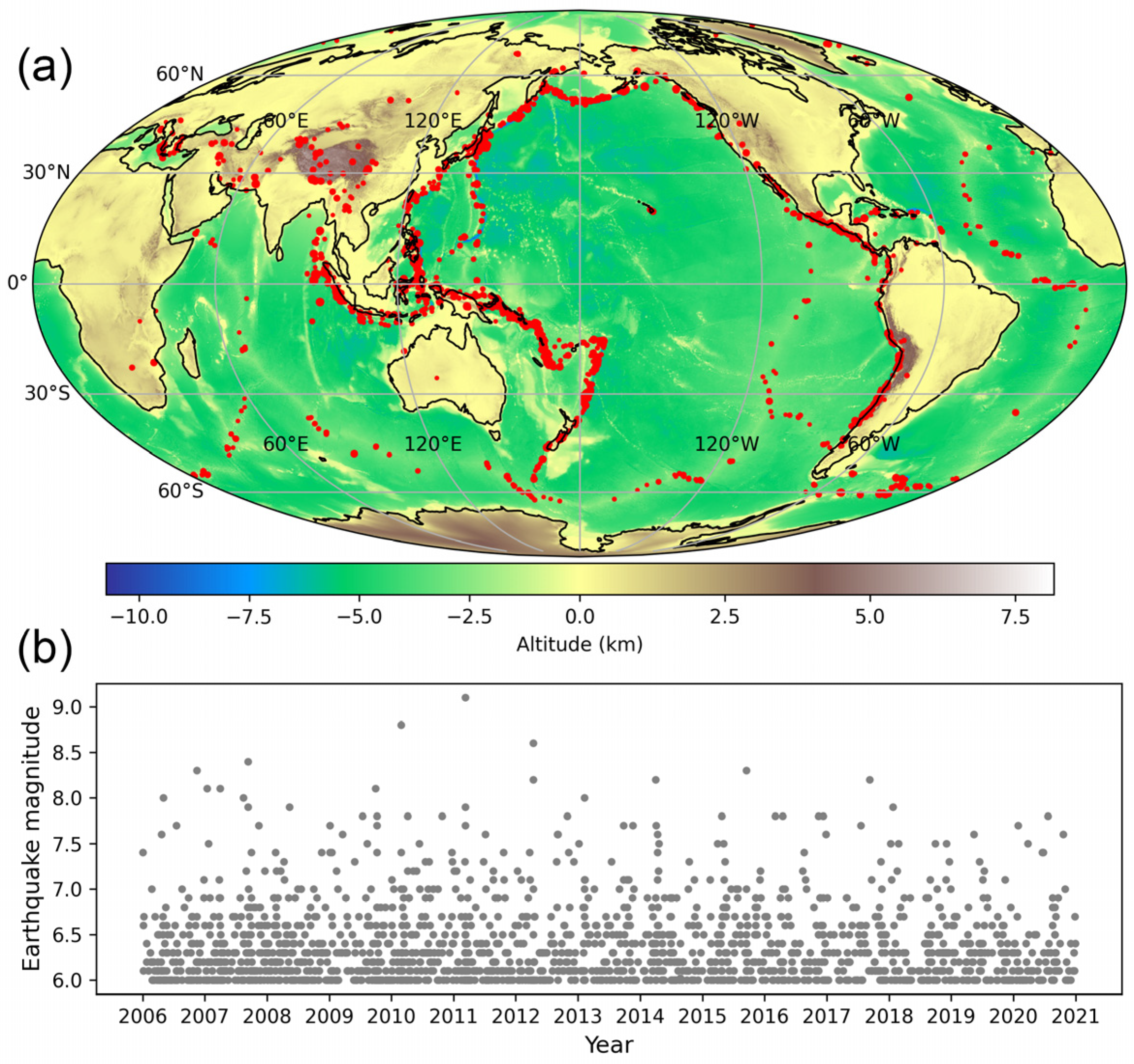
The United States Geological Survey (USGS) Earthquake Hazards Program is committed to investigating the spatial and temporal characteristics and the tectonic mechanisms of earthquakes. For this study, earthquake catalog data comprising 1825 earthquakes with a magnitude of ≥6 and focal depths of ≤70 km between 2006 and 2020 were utilized from USGS. Shallow earthquakes were selected owing to their greater damage potential and significant anomalous variations, as highlighted by previous studies [26,27]. The spatial distribution and magnitudes of the chosen earthquakes over a 15-year period are presented in Figure 1. They are observed to occur predominantly along the main plate boundaries and mid-ocean ridges. These regions are characterized by heightened plate movements and higher frequencies of seismic and volcanic activities, as reported by Jenkins et al. [28].
2.2. AIRS/Aqua Level 3 Product
The AIRS instrument, which is a new generation of high spectral resolution infrared sounder with 2378 channels, is onboard the Aqua satellite of the Earth Observation System. It was launched on 4 May 2002 and can observe the emitted infrared radiation of the earth–atmosphere system in three spectral bands: 3.74–4.61 µm (2169–2674 cm−1), 6.20–8.22 µm (1217–1613 cm−1), and 8.8–15.4 µm (649–1136 cm−1). With a horizontal spatial resolution of 13.5 km at the nadir, increasing to 41 × 21.4 km2 at the maximum zenith angle, AIRS is capable of providing a temporal resolution twice per day with a swath width of 1650 km, which covers over 95% of the Earth’s surface per day [29]. The radiances observed by AIRS can be used to estimate geophysical and geochemical parameters, including surface temperature, atmospheric temperature, water vapor content, trace gases, cloud parameters, and dust parameters. The AIRS/Aqua L3 daily standard physical retrieval (AIRS3STD) V7.0 product was utilized to compute pre-seismic multiparametric anomalies, which has a spatial resolution of 1°, and only nighttime data were considered in a daily temporal resolution. The used parameters consisted of skin temperature (ST; K), air temperature (AT; K), total integrated column water vapor burden (CWV; kg/m2), outgoing longwave radiation flux (OLR; W/m2), and clear-sky OLR (COLR; W/m2).
3. Methods
3.1. Anomaly Detection Method
Anomaly detection is the process of identifying outliers from the normal or long-term average reference values of specific geophysical and geochemical parameters, such as surface temperature and OLR, in a spatial or temporal domain. These outliers serve as indicators of potential pre-seismic anomalies, which are anomalous fluctuations that are triggered to some extent by seismogenic processes. These anomalies can be detected through diverse methods for the first step of earthquake-related anomaly recognition [27]. In this study, a z-score (ZS) normalization method was utilized, represented as follows:
where represents the current value of a given parameter (e.g., OLR) at a specific location and time t. The average and standard deviation of the reference field are calculated at the same or similar time intervals over multiple years at the location . The widely used ZS method has a simple formula that provides a clear mathematical interpretation—it is the multiple of the value from the average condition with respect to the amplitude of variation. The anomaly represents the difference between retrieved from satellite data and of the reference field over a long-term average trend. The anomalous results calculated by the ZS method are only meaningful when is not zero or is not significantly close to zero. If we consider the occurrence of anomalies as a normal distribution, the anomalies calculated by Equation (1) with values of 1, 2, and 3 represent probabilities of 68.17%, 99.45%, and 99.73%, respectively. Larger anomalies imply a higher likelihood of rare events occurring. From another perspective, the difference between and of the reference field represents the signal, and of the reference field is the noise. The higher the signal-to-noise ratio, the greater the possibility of anomalies prior to an earthquake.
3.2. Anomaly Recognition Criteria
The anomalous signals associated with earthquakes can be subtle and transient due to various natural and anthropogenic processes that significantly influence the calculated anomalies based on Equation (1) [30]. Therefore, it is essential to have a set of anomaly recognition criteria to determine whether the anomalies are caused by seismogenic processes as much as possible. The availability of anomalous perturbances prior to upcoming earthquakes largely depends on the quality of remote sensing products and anomaly detection approaches. To enhance reliability or reduce false positive rates indicated by pre-seismic anomalies, a variety of conditions or limits have been proposed [10,21]. In previous work, Jiao and Shan [25] fixed the anomaly recognition criteria at the global scale, ignoring the spatial differentiation of pre-seismic anomalies due to various tectonic environments and earthquake preparatory conditions. Therefore, to improve the earthquake forecasting capability, different values of each parameter in anomaly recognition criteria can be chosen and adapted to our framework through comparison with previous works. The following parameters and their respective potential values have been selected:
- The temporal range for warning about impending earthquakes prior to the current day is 30, 60, 90, 120, or 150 days;
- A pixel with an absolute anomaly value, which is calculated by the ZS method, of ≥1, 1.5, 2.0, 2.5, 3.0, or 3.5 will be considered a valid anomaly pixel;
- Within the sliding window, the number of valid anomaly pixels must be ≥5%, 10%, 20%, 30%, 40%, or 50% inside a 1-day resolution anomaly window;
- Within an observation period (e.g., 90 days), if there are days where ≥5%, 10%, 20%, 25%, 30%, 40%, or 50% satisfy the above conditions, a pre-seismic anomaly is identified based on daily AIRS data. For instance, if there are more than 9 days (i.e., 90 days × 10%) within a 90-day period that meet the specified conditions, an anomalous event is confirmed.
Additionally, a sliding spatial window of 7° × 7° surrounding a central grid of 1° spatial resolution was used in this study. When a pre-seismic anomaly is identified at a specific time and position, an alarm warns that a M ≥ 6 earthquake is likely to occur within the next 30 days within the sliding spatial window. For each pixel with 1° spatial resolution at a global scale, a set of specified parameters is optimally determined, using the approach described in Section 3.4.
3.3. Metrics to Evaluate Earthquake Forecasting Capability
To evaluate the earthquake forecasting capability of pre-seismic anomalies from AIRS data, a comprehensive indicator, Matthew’s correlation coefficient (MCC), was used. MCC is a statistical index that is more reliable than accuracy and F1 score for binary classification evaluation. It is relatively balanced and provides a high score only when predictions have good results in all four confusion matrix categories (i.e., true positives, true negatives, false positives, and false negatives), thus avoiding overoptimistic assessment results found in other statistical rates [31]. When using equivalent terms that are directly related to earthquake forecasting [25], MCC is redefined as
where Acc denotes the accuracy forecasting count, Nor is the normal count, Fal represents the false alarm count, and Mis is the missed detection count. The MCC value ranges from −1 to 1, with 1 indicating perfect earthquake forecast, 0 meaning that the proposed model is no better than a random guess, and −1 denoting exact opposite prediction results.
MCC values from −1 to 0 are considered invalid because they denote a normal condition (i.e., no earthquakes) when anomalies occur. This contradicts the assumption that various anomalous phenomena observed during the seismogenic stage are generated by underlying fault activity that triggers impending earthquakes. Additionally, when calculating the global mean condition, positive and negative MCC values counteract each other, leading to problematic statistical outcomes. Furthermore, if we are to consider the negative MCC of a pixel in seismically active regions, we could alter the anomaly recognition criteria in the opposite direction to achieve valid earthquake forecasting. While this approach may be statistically feasible, it may impede the exploration of the underlying geophysical mechanism through satellite observations and ground measurements. This raises concerns about the prevalence of anomalous fluctuations and the calm phase before earthquakes that are perceived as accidental occurrences. Consequently, from this perspective, anomaly detection methods relying on a reference field for long-term averages become devoid of meaningful basics. The consideration of negative MCC values as invalid still remains an open question that necessitates further investigation to ascertain its reasonability and implications.
3.4. Determination of Spatially Self-Adaptive Anomaly Identification Parameters
To obtain the optimal anomaly recognition criteria for each pixel with a 1-degree spatial resolution, a local self-adaptive scheme was proposed. Firstly, nighttime data of multiparameter anomalies within a 7 × 7 sliding window for a single day are extracted from the period of 2006 to 2020, generating a spatiotemporal data cube for the central pixel. Secondly, the possible values of four parameters described in Section 3.2 are iteratively applied to the data cube, and the combination of parameter values with the highest MCC value is selected as the final optimal parameters for that pixel. Finally, the calculations are applied to each pixel through the sliding window, and optimal parameters are gridded to indicate their spatial distributions. There are 1800 loops (i.e., 5 base days × 6 absolute anomaly values × 6 anomaly ratios × 6 anomaly counts) for each pixel globally (180 × 360 pixels), and, due to the overwhelming computation cost, limited discrete values of parameters of the anomaly recognition criteria are used in this study to relieve computational constraints. It should be noted that anomalies of the five used geophysical parameters (ST, AT, CWV, COLR, and OLR) of the AIRS product require independent optimal parameters.
To prevent overfitting, a 3-fold cross-validation was conducted on the training set to fine-tune the anomaly identification parameters and determine the optimal parameter configuration. The spatiotemporal data cube was divided into three consecutive folds, consisting of a training set and a test set (Table 1). Each fold was utilized as a validation set once, while the remaining two folds constituted the training set. The optimal parameters were determined using all the data in the training set, and the earthquake forecasting capability was evaluated using the test data set. Note that this study utilized data from only 1825 earthquakes occurring over a 15-year period. A higher number of folds in cross-validation leads to fewer earthquakes being used in the test dataset. For instance, in the case of 5-fold cross-validation, only earthquakes from a 3-year period were used to assess earthquake forecasting capability. In seismically active regions, calculating the MCC may encounter challenges due to the rarity of strong shocks occurring at the same location (i.e., one pixel) within a relatively short period. From a statistical standpoint, this can lead to unstable results. As a tradeoff, we selected 3-fold cross-validation to increase the number of earthquake cases in the test dataset, and to also have the ability to assess the reliability of our proposed approach with different folds.
4. Results
4.1. Optimal Parameters of Anomaly Recognition Criteria
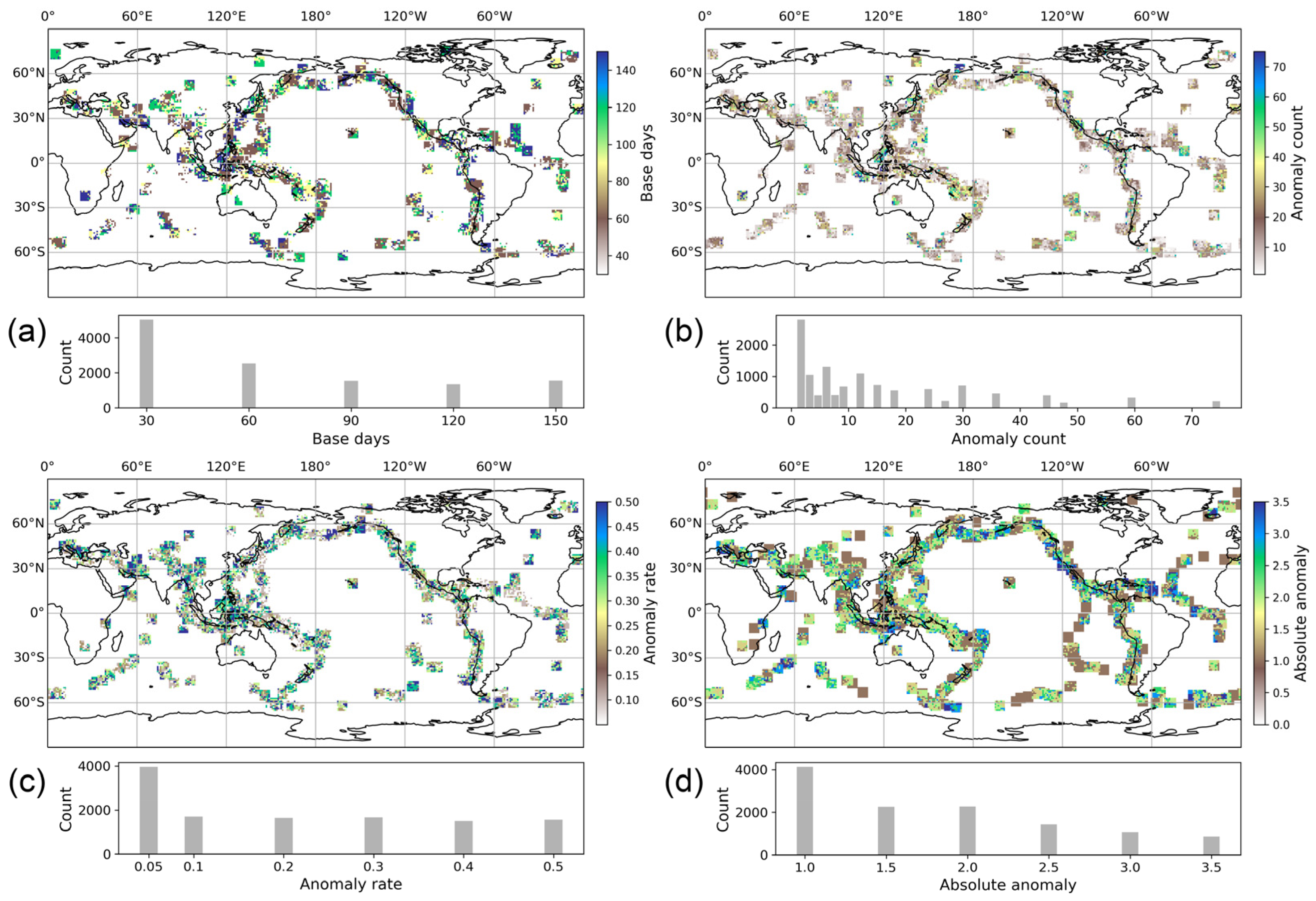
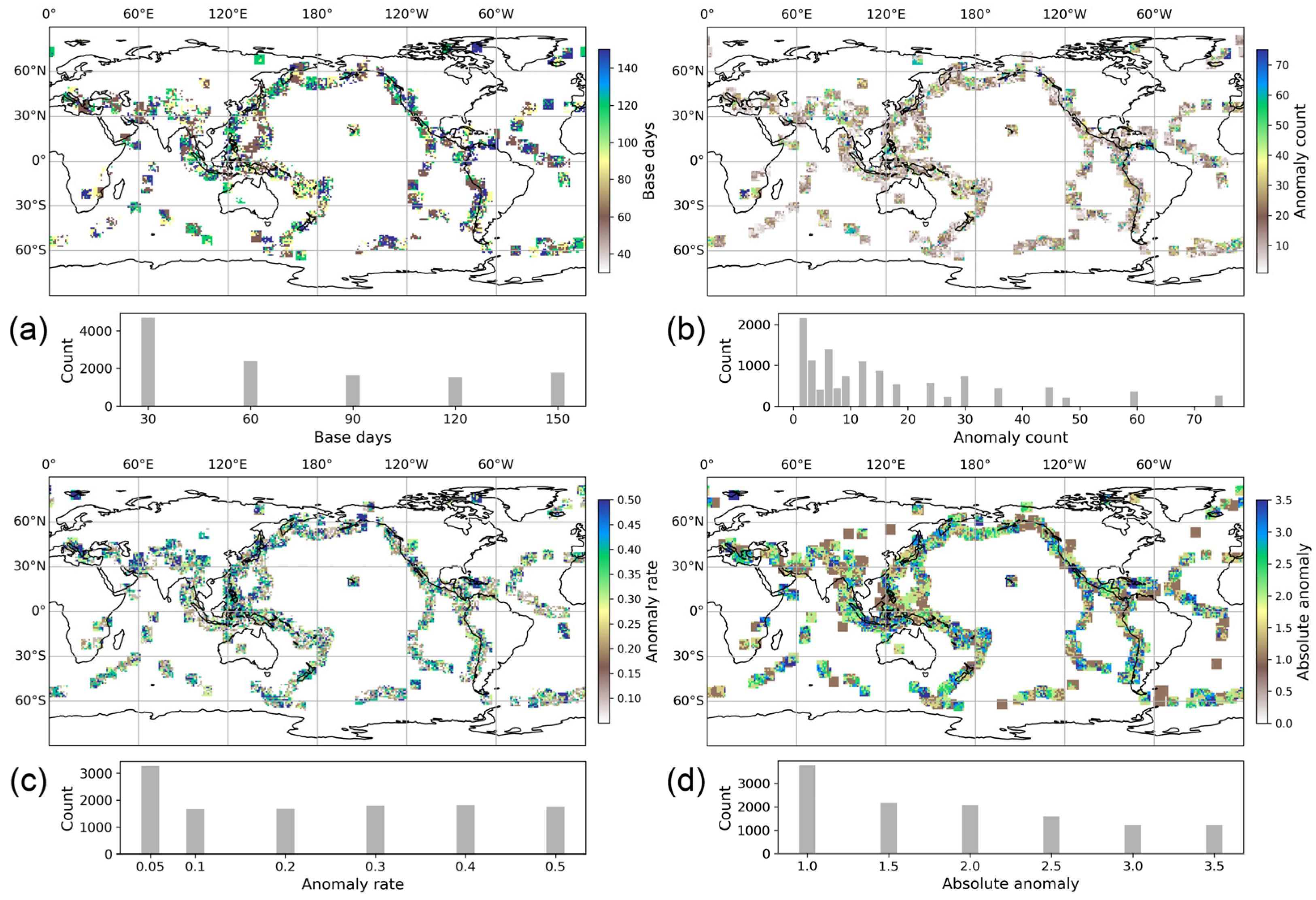
The optimal parameters for anomaly recognition criteria in Section 3.2 were determined using a spatially self-adaptive anomaly identification scheme, as depicted in Figure 2, for AIRS OLR anomalies using training data within 2011–2020. Each optimal parameter exhibited significant spatial variation in seismically active regions, and their values tended to become lower, indicating that most pre-seismic anomalies are short-term and subtle signals, which makes it harder to identify seismic-related anomalies prior to major earthquakes. The largest number of base days was for 30 days, while the 60- and 90-day values dominated seismically active regions in China (Figure 2a). A previous study about the multiple anomalies before the 2015 Nepal earthquake sequence summarized by Wu et al. [30] showed similar characteristics. The anomaly count was calculated using a fixed ratio of base days, and, due to the lower values of base days, anomaly counts over most areas were less than 30 (Figure 2b). Therefore, recognizable anomalies that forecast impending earthquakes are not very frequent, the same as was seen for the identified thermal anomalies in relation to earthquakes by Filizzola et al. [32]. In Figure 2c, the values of anomaly ratio (i.e., the ratio between the number of pixels that have anomalies occurred and total pixels in a 7° × 7° window) have relatively equal counts except for the anomaly ratio value of 0.05. The absolute anomaly values were always less than 3.0 (Figure 2d), indicating generally weak anomalous signs that are possibly associated with imminent earthquakes. This threshold value is always adopted by studies when using analogical anomaly detection methods [27]. Given that the anomalous values follow a normal distribution, the valid absolute anomaly values account for a 99.7% probability, according to Equation (1), meaning that it is a non-trivial probability event. The statistical results also reveal that the recognition capability of a temporal integrated anomaly method can outperform random guessing [33].
Although the spatiotemporal evolution patterns of earthquake-related anomalies have not been definitively ascertained (i.e., no widespread consensus yet), our research provides a quantitative description of the characteristics of pre-earthquake anomalies or seismic precursory signals through the use of four criteria (see Section 3.2). The optimal results obtained from these criteria represent the most likely possibility for forecasting earthquakes (Figure 2), and their respective values offer insights into the subtlety and short-term nature of seismic precursory signals, thereby emphasizing the complexities involved in identifying seismic-related anomalies. To further establish the connection between these signals and seismic activity, we analyzed the MCC results, as shown in the subsequent sections. MCC serves as a metric to represent the possibility of earthquake forecasting based on anomalous phenomena, with higher MCC values suggesting a stronger likelihood of a robust connection between the identified precursory signals and seismic events. This analytical approach allows us to gain a more comprehensive understanding of the efficacy and potential of using seismic precursors for earthquake forecasting, further validating the relevance and significance of our research findings.
In addition, we employed 3-fold cross-validation to estimate the optimal parameters of the anomaly recognition criteria. The results obtained for different training periods are presented in Figure A1 and Figure A2 in the Appendix A. The spatial distributions of the optimal parameters exhibited minimal variations among each other, and their histograms demonstrated a high level of consistency. This indicates that the calculation method used to obtain the optimal parameters for the anomaly recognition criteria is relatively reliable. Therefore, in this study, we present the results only for the first fold of cross-validation. The results for the anomalies of AIRS ST, AT, CWV, and COLR displayed similar characteristics and are, therefore, not shown.
4.2. Optimal Parameters of Multiparameter Composed Anomalies
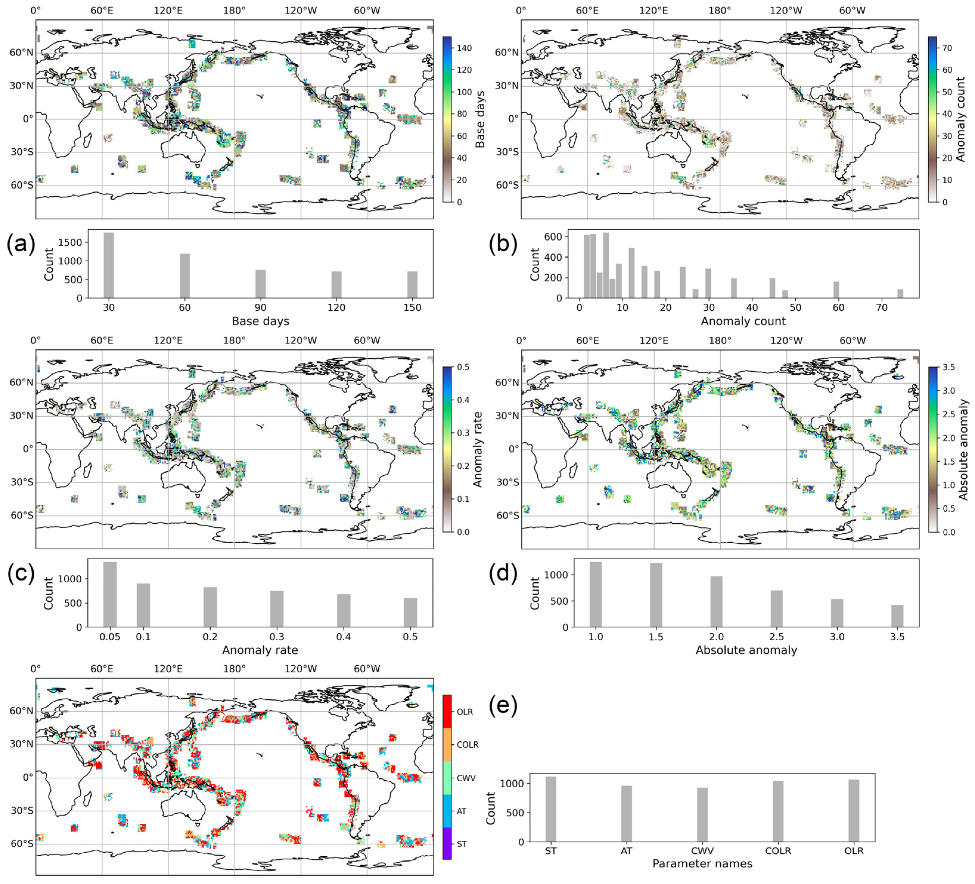
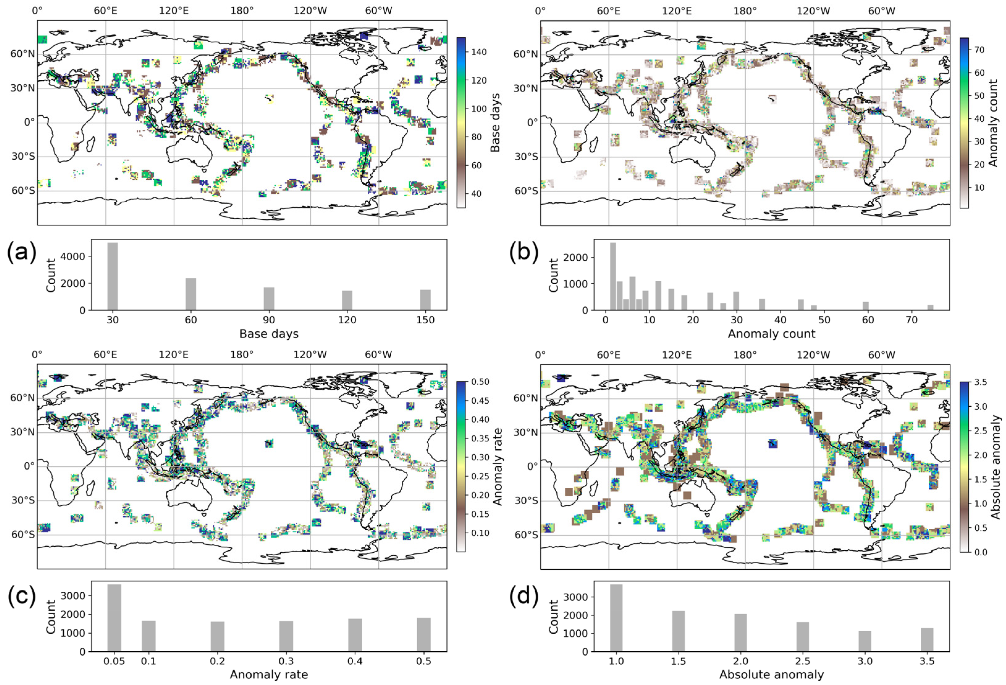
To enhance earthquake forecasting capacity, a simple composition method was utilized to select the optimal anomaly parameter for a pixel based on the best MCC value at the test stage for the years 2006–2010. This approach ensures that a region not only possesses the best anomaly recognition criteria, but also the dominant geophysical parameter that generates the most effective earthquake forecasting capability based on its anomalous variations prior to impending earthquakes. The spatial distributions and histograms of optimal parameters for composed (COM) anomalies are illustrated in Figure 3. Anomaly recognition criteria exhibited analogous statistical characteristics to those in Figure 2. Optimal parameters at some pixels obtained at the training stage cannot generate valid forecasting (i.e., MCC ≤ 0) at the test stage, causing less predictable areas, as shown in Table 2. The results with different training periods under a 3-fold cross validation are shown in Figure A3 and Figure A4.
The key information from optimal parameters for such composed anomalies was that the dominant geophysical parameter at the global scale is OLR, encompassing all-sky and clear-sky OLRs, as displayed in Figure 3e with red and orange areas. The secondary parameter is ST, whereas CWV and AT have a minimal percentage. The implication is that OLR anomalies could prove to be a more viable candidate for global earthquake forecasting under the background of the consideration that a multi-parametric strategy holds promise in advancing the development of seismic forecasting [21]. The findings presented by Fu et al. [22] offer compelling evidence that OLR may serve as a potential indicator for forecasting earthquakes in the Taiwan region. OLR refers to the total longwave radiation emitted from the Earth–atmosphere system at the top of the atmosphere in a spectral range of 4 to 100 µm. It is primarily influenced by surface temperature and emissivity, atmospheric profile of temperature and water vapor, clouds, and greenhouse gases. From the perspective of the lithosphere–atmosphere–ionosphere coupling mechanism [30,34], OLR represents an integrated effect of anomalous fluctuations that occur within the seismogenic zone, spanning from the lithosphere to the atmosphere. Therefore, OLR anomalies could be a delegate of the gross effect beneath the top of the atmosphere (e.g., air temperature anomalies).
4.3. MCCs of AIRS Multiparameter Anomalies Using Optimal Parameters
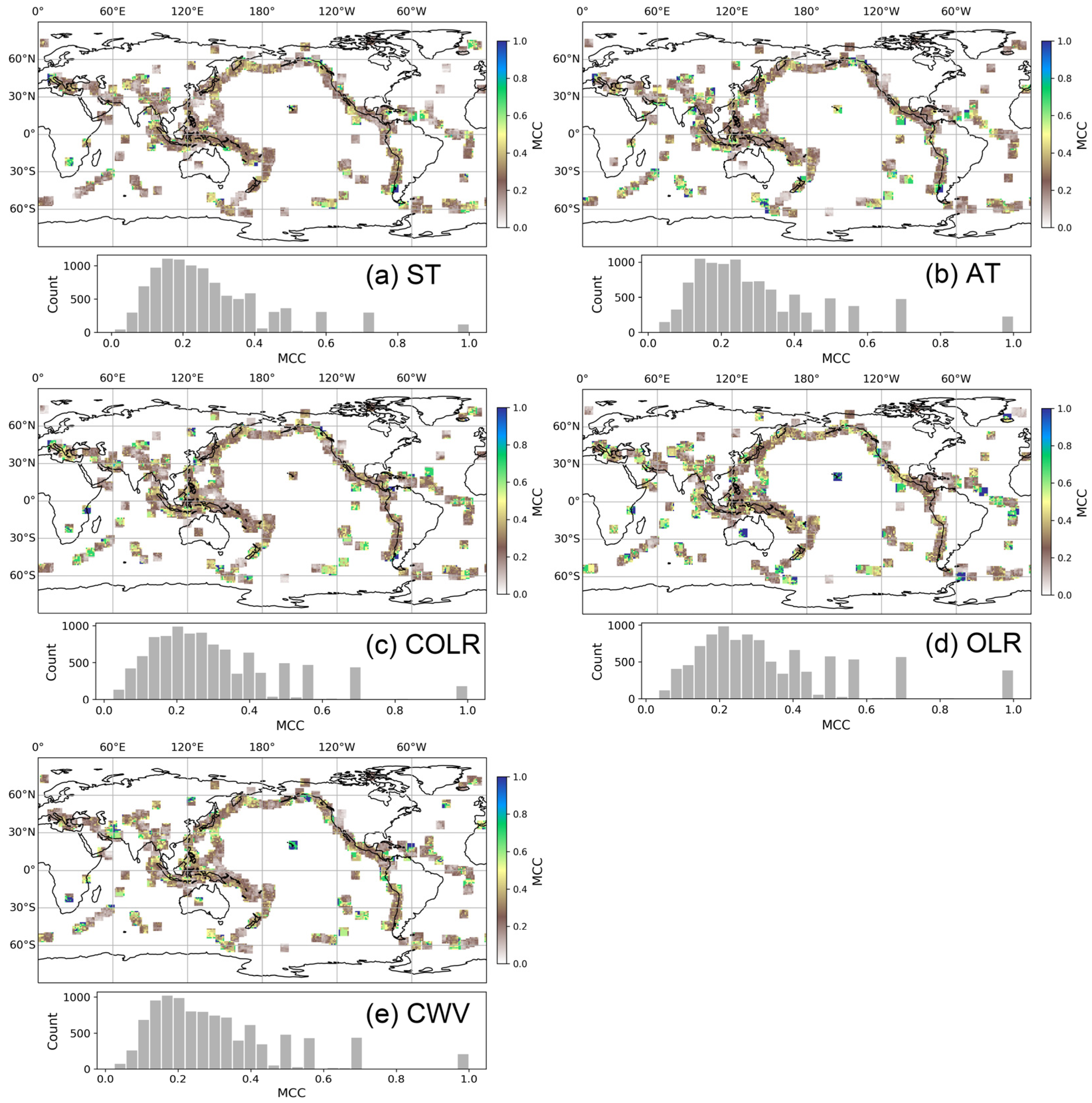
During the training stage, most pixels within the seismically active regions demonstrated valid forecasting capability, as indicated by a MCC greater than 0, shown in Figure 4 and summarized in Table 2. This finding indicates that the optimal parameters of anomaly recognition criteria effectively forecast earthquakes within the period from 2011 to 2020 for most seismically active regions. Interestingly, certain regions exhibited particularly high MCC values exceeding 0.5, as depicted by the bright yellow and green areas. These regions were widely distributed without following any specific spatial pattern. The histograms of MCC values for each parameter anomaly demonstrated a similar characteristic, with most areas having MCC values below 0.4, an average MCC of approximately 0.2, and only a few regions with MCC values exceeding 0.5. Moreover, the spatial distribution of MCC values varied among different geophysical parameters, as illustrated in Figure 4. This suggests the potential for a complementary effect, where different anomalies may combine to improve earthquake forecasting capabilities. These observations provide valuable insights into the spatial patterns and distribution of forecasting skill, paving the way for further research and potential enhancements to earthquake forecasting methodologies.
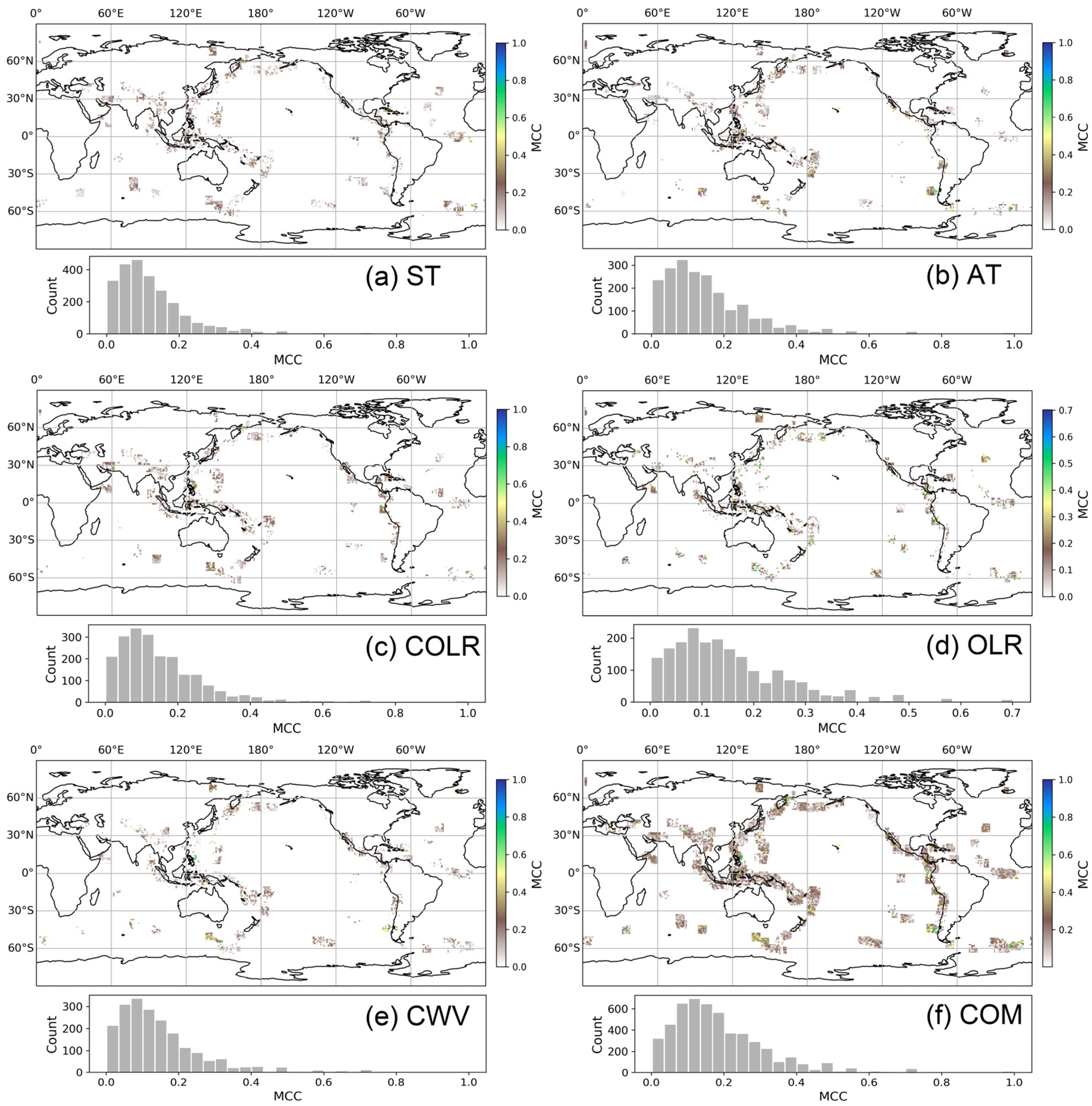
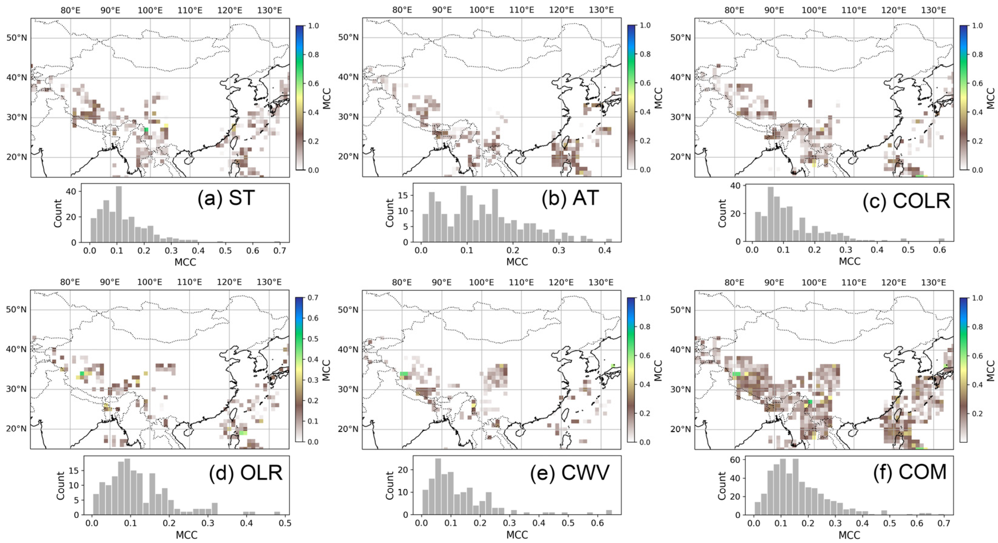
Figure 5 presents the spatial distribution and statistical histograms of the MCC, which depict the seismic forecasting performance of five geophysical parameters derived from AIRS during the test stage spanning from 2006 to 2010. In comparison to the results obtained during the training stage (Figure 4), fewer regions demonstrated valid forecasting capabilities. This can be attributed to the limited occurrence of earthquakes with a magnitude of ≥6 and focal depths of ≤70 km between 2006 and 2010, as the calculation of MCC requires an adequate number of earthquake cases for reliable evaluation. Furthermore, it is noteworthy that similar spatial distributions of MCCs as well as the statistical results in Table 2 were observed across different anomalies of geophysical parameters. The average MCC values ranged from 0.122 for ST anomalies to 0.152 for OLR anomalies. The valid ratios at the test stage ranged from 0.164 for OLR anomalies to 0.200 for ST anomalies. These results exhibited a significant decrease compared to those at the training stage (Table 2), where the average MCC values ranged between 0.272 and 0.338, with a ratio of 0.836. However, despite the decrease in performance during the test stage, it is important to recognize that our proposed scheme is still capable of capturing to some extent the underlying mechanism of earthquake occurrences. The challenging nature of earthquake forecasting in the time period, characterized by a scarcity of relevant events, contributes to the observed decrease in forecasting capability. Nonetheless, the insights gained from these results contribute to a deeper understanding of the complexities involved in earthquake forecasting and offer valuable directions for further research and improvements to our methodology.
The MCCs of composed anomalies showed significant improvement due to the increase in the number of predictable regions from ~0.175 to 0.424 in Table 2. On average, the MCCs increased from 0.143 (average of all geophysical parameters) to 0.186 when composed anomalies were applied. These values may not be high enough to meet the requirements of an operational earthquake forecasting system. Machine learning-based methods have demonstrated the capability to achieve higher MCC values [35], despite employing different earthquake cases and distinct data processing approaches. Nevertheless, the simple composite scheme demonstrates the effectiveness of applying multiparametric anomalies and is feasible for improving the earthquake forecasting capability. Previous studies have suggested the integration of different precursors of lithosphere, atmosphere, and ionosphere to promote reliable earthquake forecasting [6,7,36]. Our proposed scheme provides a probable and sustainable path towards achieving this goal.
5. Discussion
5.1. Comparison with the Results Obtained Using Fixed Anomaly Recognition Criteria
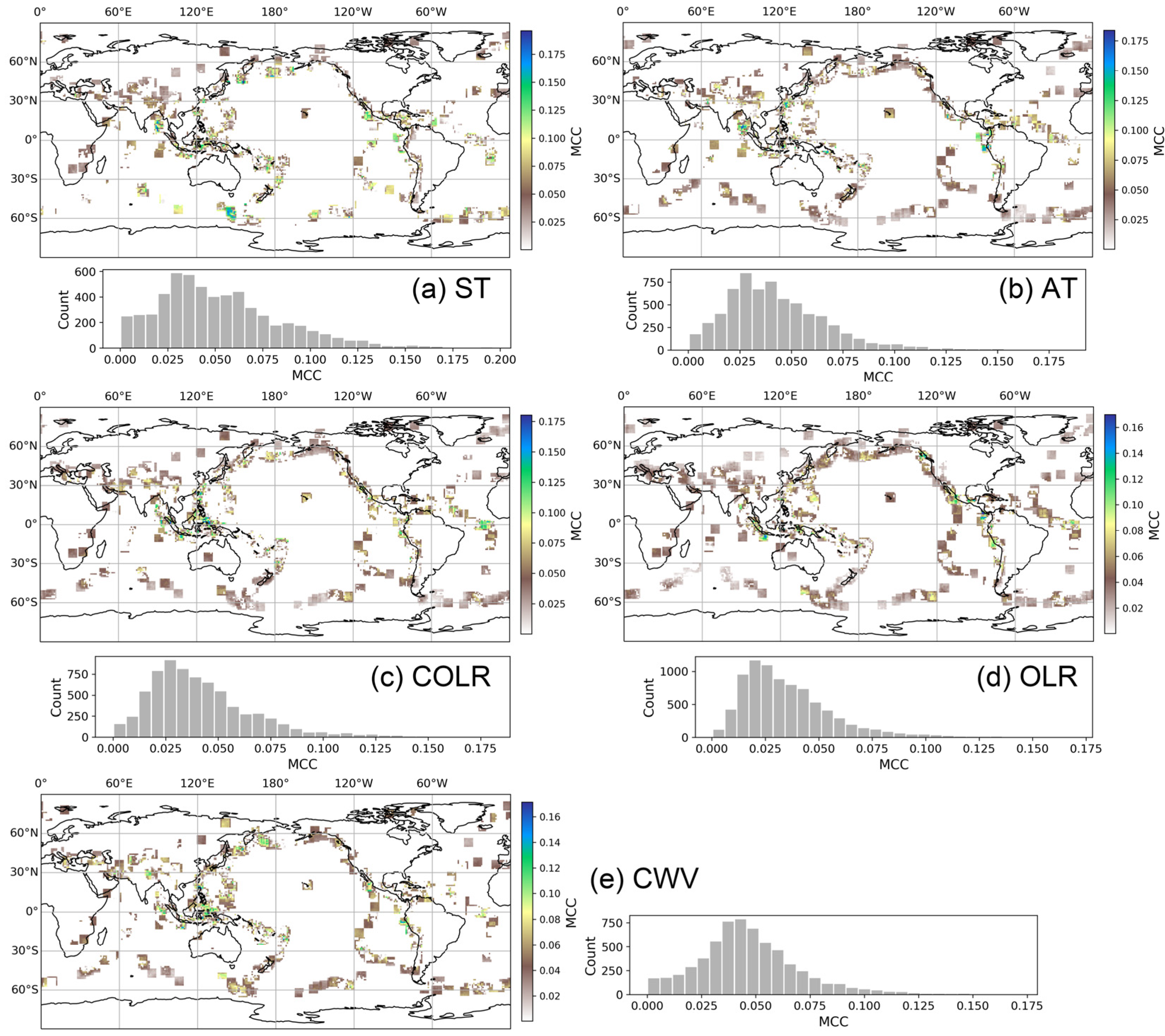
In contrast to fixed anomaly recognition criteria, the spatially self-adaptive anomaly identification scheme demonstrates significant improvements. Figure 6 illustrates that the fixed criterion lacks adaptability, resulting in relatively low MCC values (averaging less than 0.05) for a significant portion of seismically active regions. These low values indicate inaccurate predictions, where pre-seismic anomalies are not followed by earthquakes. Consequently, the fixed criteria fail to identify pre-seismic anomalies in these areas, undermining the reliability of earthquake forecasting. Conversely, the optimal parameters of the local self-adaptive scheme generate higher MCC values (at least greater than 0.12), as shown in Table 2 for the majority of seismically active regions (Figure 5). This crucial advancement represents a significant improvement in producing reliable earthquake forecasts.
5.2. MCCs of Inland, Coastal, and Oceanic Earthquakes
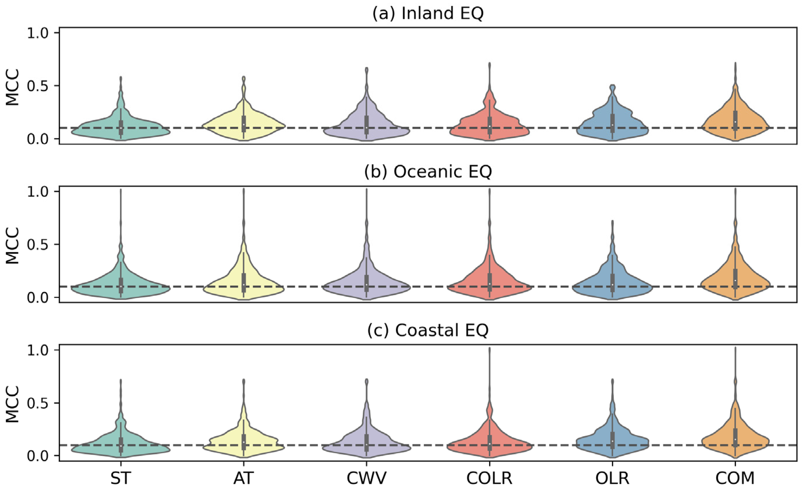
The earthquakes investigated in this study were categorized into three types based on their location: inland, coastal, and oceanic events. The MCC histograms presented in Figure 7 reveal that the location of earthquakes has a limited influence on the earthquake forecasting performance of each AIRS parameter anomaly. Specifically, for inland earthquakes, there is a scarcity of samples with higher MCC values. However, for all geophysical parameters, except for OLR, the maximum MCC value can reach 1.0. Across all five geophysical parameters, the majority of MCC values are below 0.5. Nevertheless, when considering the combined anomalies, the overall average MCC can reach 0.186 (Table 2). The MCC histograms of the same geophysical anomaly for the three types of earthquakes exhibit similar patterns, indicating that earthquake location does not affect the forecasting capability too much. The statistical results are presented in Table 3, revealing that oceanic earthquakes consistently exhibit slightly higher mean MCC values for each parameter, albeit with limited increments. This demonstrates that the use of composed anomalies results in a significant improvement of approximately 0.043 in MCC on average, compared to the use of a single geophysical parameter. This improvement is independent of the type of earthquake location, including inland, oceanic, and coastal earthquakes (Figure 7). Our previous research [33] also reveals that statistical characteristics based on earthquake focal mechanisms do not exhibit significant differences, despite the use of different approaches and earthquake events. This suggests that the geophysical mechanism underlying the generation of anomalous signals prior to upcoming earthquakes is possibly consistent across earthquake types and locations [34,37].
5.3. Earthquake Forecasting Capability of Pre-Seismic Anomalies in China Mainland
China Mainland is a region known for its susceptibility to seismic activity, characterized by strong and shallow earthquakes that can cause substantial damage. The frequent occurrence of earthquakes in China necessitates the ability to forecast impending seismic events in the short term, typically within a span of several weeks. This forecasting capability is crucial for minimizing potential risks associated with earthquakes and their secondary hazards, such as landslides and debris flow [38]. Figure 8, which specifically focuses on China and its immediate vicinity, reveals that the MCC of individual geophysical parameters typically ranges between 0 and 0.4. Valid anomalies primarily occur along the Qinghai–Tibet Plateau and the south–north seismic belt, both being prominent regions with significant seismic activity [39]. When considering the combination of all geophysical parameters, a greater number of areas in midwestern China, the region with the highest seismic activity, exhibit higher MCC values, averaging around 0.15.
5.4. A Statistical Evaluation Framework for Earthquake Forecasting
In this study, we have developed a spatially self-adaptive multiparametric anomaly identification scheme based on global strong earthquakes, building upon recent advancements in earthquake forecasting research. Our scheme represents a notable improvement over conventional methods that employ fixed anomaly recognition criteria. Additionally, we have incorporated a simple composed approach, further enhancing the earthquake forecasting capability of the proposed scheme. These findings underscore the significance of our approach in advancing earthquake forecasting methodologies. When considering the application of these results to operational earthquake forecasting, the generated global MCC map, in conjunction with new observation data, can serve as a valuable reference for assessing the reliability or probability of anomalous events to indicate upcoming earthquakes. This integrated approach can enhance the credibility and confidence in identifying significant anomalies in earthquake forecasting endeavors.
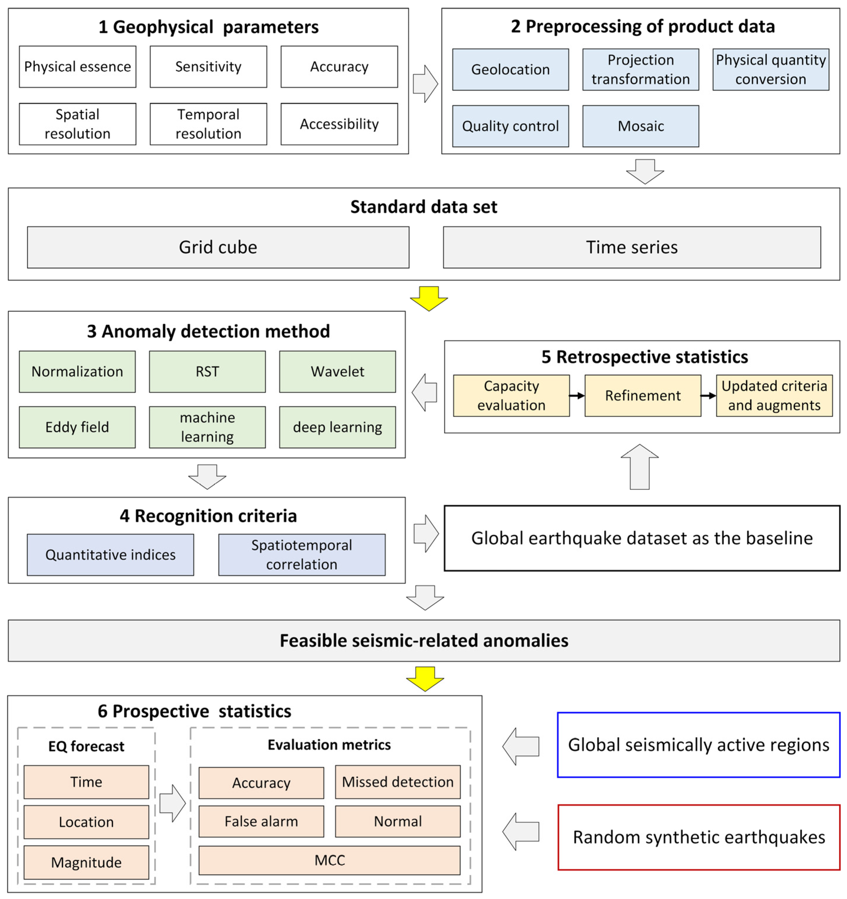
This scheme plays a pivotal role within our proposed statistical evaluation framework for earthquake forecasting, as illustrated in Figure 9 [20,25]. It aims to enhance the recognition of pre-seismic anomalies that are potentially associated with impending strong earthquakes (Parts 3, 4, and 5 in Figure 9), specifically focusing on earthquakes with a magnitude greater than six in this study. This focus on strong earthquakes is supported by several recent studies [6,40], which highlight the significance of early detection and accurate forecasting for such events. To evaluate the earthquake forecasting capability in a more comprehensive manner, we introduced the use of random synthetic earthquakes in the prospective statistics. This approach enables us to assess earthquake forecasting capabilities across stochastic locations worldwide and over different time periods. The effectiveness of this methodology has been demonstrated in a previous study [33], where it proved valuable in examining the performance of anomaly detection methods.
The primary objective of our framework is to provide a quantitative and consistent evaluation of the earthquake forecasting capability, encompassing various geophysical and geochemical parameters. These parameters are primarily obtained through state-of-the-art remote sensing technologies (Parts 1 and 2 in Figure 9), coupled with advanced anomaly detection methods (Part 3). This holistic approach sets our study apart from traditional case studies prevalent in the literature. Recent publications [25,30] emphasize the need for comprehensive evaluation frameworks that incorporate diverse parameters and anomaly detection techniques. Through this simple yet robust framework, we aim to identify the optimal parameters and anomaly detection methods for earthquake forecasting. While the accurate forecast of earthquakes remains a significant challenge, the evaluation metrics, such as the MCC, allow us to estimate the most plausible lower limits of forecasting performance. Any advancements achieved exceeding these lower limits are crucial steps toward advancing operational earthquake forecasting.
5.5. Challenges and Possibilities of Current Scheme
We employed five geophysical parameters derived from AIRS observations to compute pre-seismic anomalies and forecast impending strong earthquakes. As a high spectral resolution infrared sounder, cloud cover significantly affects the availability of data in the AIRS3STD product. Consequently, missing data during the observation period can lead to gaps in anomalous results and altered historical data that affect the calculation of the reference field, subsequently impacting the forecasting state (i.e., accurate forecast, normal condition, false alarm, or missed detection), as specified in Section 3.2. This, in turn, can influence the MCC of a given geophysical parameter. To address this issue, we will incorporate reanalysis data from sources such as the European Centre for Medium-Range Weather Forecasts Reanalysis v5 (ERA5). ERA5 datasets offer seamless spatiotemporal coverage for the relevant geophysical parameters, enabling us to validate and refine our proposed forecasting scheme. Furthermore, this will allow us to investigate the influence of gaps in the product data, providing valuable insights into their potential impact on earthquake forecasting capability.
The quality of the utilized AIRS product is a crucial aspect, given that these data products have undergone extensive development and validation over the years, resulting in their increased maturity (https://airs.jpl.nasa.gov/data/guides-docs, accessed on 28 July 2023). While the validation of various geophysical parameters of the AIRS product is beyond the scope of this study and constitutes a vast topic on its own, it remains an essential consideration. Nevertheless, it is worth noting that, if the data product exhibits no systematic biases, the ZS method employed in this study can mitigate certain retrieval errors by employing the manipulation of the difference and ratio, as presented in Equation (1). This issue also holds significance for other retrieved parameters, as retrieval algorithms typically involve simplifying assumptions to model complex physical processes, inevitably introducing retrieval errors. The uncertainties stemming from these assumptions can significantly impact anomaly detections and even earthquake forecasting, yet their precise extent remains unclear.
The optimal parameters for anomaly recognition criteria were determined using 3-fold cross-validation. This approach was adopted to mitigate the significant overfitting issue that arises when utilizing all 1825 earthquakes to estimate the optimal parameters. The overfitting problem adversely affects earthquake forecasting for the years 2021 and 2022, resulting in low MCC values, which are not presented in this paper. The application of cross-validation in our study effectively improved the overfitting problem, as demonstrated in Section 4.3. However, achieving a set of unified optimal parameters still requires the implementation of specific optimization methods. The primary challenge in this context stems from the limited number of available earthquakes for analysis. Consequently, we must derive the best model based on a small number of samples. This limitation becomes even more critical when employing deep learning methods that demonstrate its advantage in forecasting earthquakes [35], as they typically necessitate a large number of training samples to yield meaningful results [41]. As a result, it is imperative to carefully address this constraint when considering the use of deep learning approaches in our research.
In recent years, probabilistic and physical earthquake forecasting systems have emerged as cutting-edge research in the field [42,43]. To enhance earthquake forecasting capabilities, a simple composed approach was adopted in this study, incorporating anomalies of multiple geophysical parameters. However, a limitation of this method is the inability to quantify the individual contribution of each geophysical parameter anomaly to the final probabilistic forecasting outcome, given the integration of multiparametric anomalies. To address this challenge, we are exploring statistical models that enable the calculation of forecasting probabilities for specific geophysical parameters, leveraging both long-term historical data and short-term observations. Subsequently, employing a multiparametric integration model becomes feasible, allowing for the calculation of earthquake occurrence probabilities in the near future. The development of operational earthquake forecasts serves as a foundation for enhancing global resilience to earthquakes, facilitating preparedness and mitigation efforts worldwide.
6. Conclusions
We have developed a spatially self-adaptive scheme to identify pre-seismic multiparametric anomalies using data from global strong earthquakes recorded between 2006 and 2020. This scheme represents a significant improvement over fixed anomaly recognition criteria, which often lead to invalid forecasts in many seismically active regions. Through our research, we have obtained optimal parameters for the anomaly recognition criteria in global seismically active regions, revealing substantial spatial variation on a global scale. The identified optimal values indicate that most anomalies associated with impending earthquakes are characterized by short-term and subtle signals with a low occurrence frequency. Moreover, we have found that the locations of earthquakes have limited impact on the earthquake forecasting capability of this scheme. Additionally, we have proposed a simple multiparametric composition approach to enhance the earthquake forecasting capability, where each geophysical parameter can contribute a distinct role to overall capability, which has demonstrated superior effectiveness compared to single-parameter approaches, as indicated by improved MCCs. The MCCs of composed anomalies have shown significant improvement in a larger number of regions, with MCC values exceeding 0.5 and an average increase from 0.143 to 0.186. Furthermore, our study has identified OLR including all-sky and clear-sky ones as the dominant geophysical parameter on a global scale, and OLR anomalies exhibit promising potential as a viable contender for earthquake forecasting.
In this study, earthquake forecasting relies on data-driven anomaly detection models that evaluate the probability and future state of imminent strong earthquakes. The results obtained provide valuable insights into our ability to forecast catastrophic earthquake events with greater accuracy. Although we have not yet achieved demonstrably successful predictions of large earthquakes, this study presents a promising approach to the development of remote sensing-based earthquake monitoring and forecasting systems.
Author Contributions
Conceptualization, Z.J.; Formal analysis, Z.J.; Funding acquisition, Z.J. and X.S.; Methodology, Z.J.; Writing—original draft, Z.J.; Writing—review & editing, Z.J., Y.H. and X.S. All authors have read and agreed to the published version of the manuscript.
Funding
This research was funded by the Basic Science Research Plan of the Institute of Geology, China Earthquake Administration, grant number IGCEA2002, and National Key Research and Development Program of China, grant number 2019YFC1509202, 2018YFC1503602.
Data Availability Statement
AIRS AIRS3STD data are available from the Goddard Earth Sciences Data and Information Services Center (GES DISC) at https://disc.gsfc.nasa.gov/datasets/AIRS3STD_7.0/summary (accessed on 2 July 2023). Earthquake catalog data are available from the United States Geological Survey (USGS) at https://www.usgs.gov/natural-hazards/earthquake-hazards (accessed on 2 July 2023).
Acknowledgments
The authors would like to acknowledge the reviewers and editors for their valuable comments and suggestions, which helped improve the quality of this work.
Conflicts of Interest
The authors declare no conflict of interest.
Appendix A
Figure A1.
The optimal parameters of the anomaly recognition criteria employed for forecasting imminent earthquakes using the outgoing longwave radiation anomaly based on training data within 2006–2010 and 2016–2020, as indicated by their spatial distributions and histograms in the top and bottom subfigures, respectively. The parameters include (a) the base days preceding earthquakes; (b) the anomaly count that occurred during the base days; (c) the anomaly rate within the spatial window, which is 7 × 7 pixels in this study; and (d) the absolute anomaly value used to identify potential earthquake-related anomalies.

Figure A2.
The optimal parameters of the anomaly recognition criteria employed for forecasting imminent earthquakes using the outgoing longwave radiation anomaly based on training data within 2006–2015, as indicated by their spatial distributions and histograms in the top and bottom subfigures, respectively. The parameters include (a) the base days preceding earthquakes; (b) the anomaly count that occurred during the base days; (c) the anomaly rate within the spatial window, which is 7 × 7 pixels in this study; and (d) the absolute anomaly value used to identify potential earthquake-related anomalies.

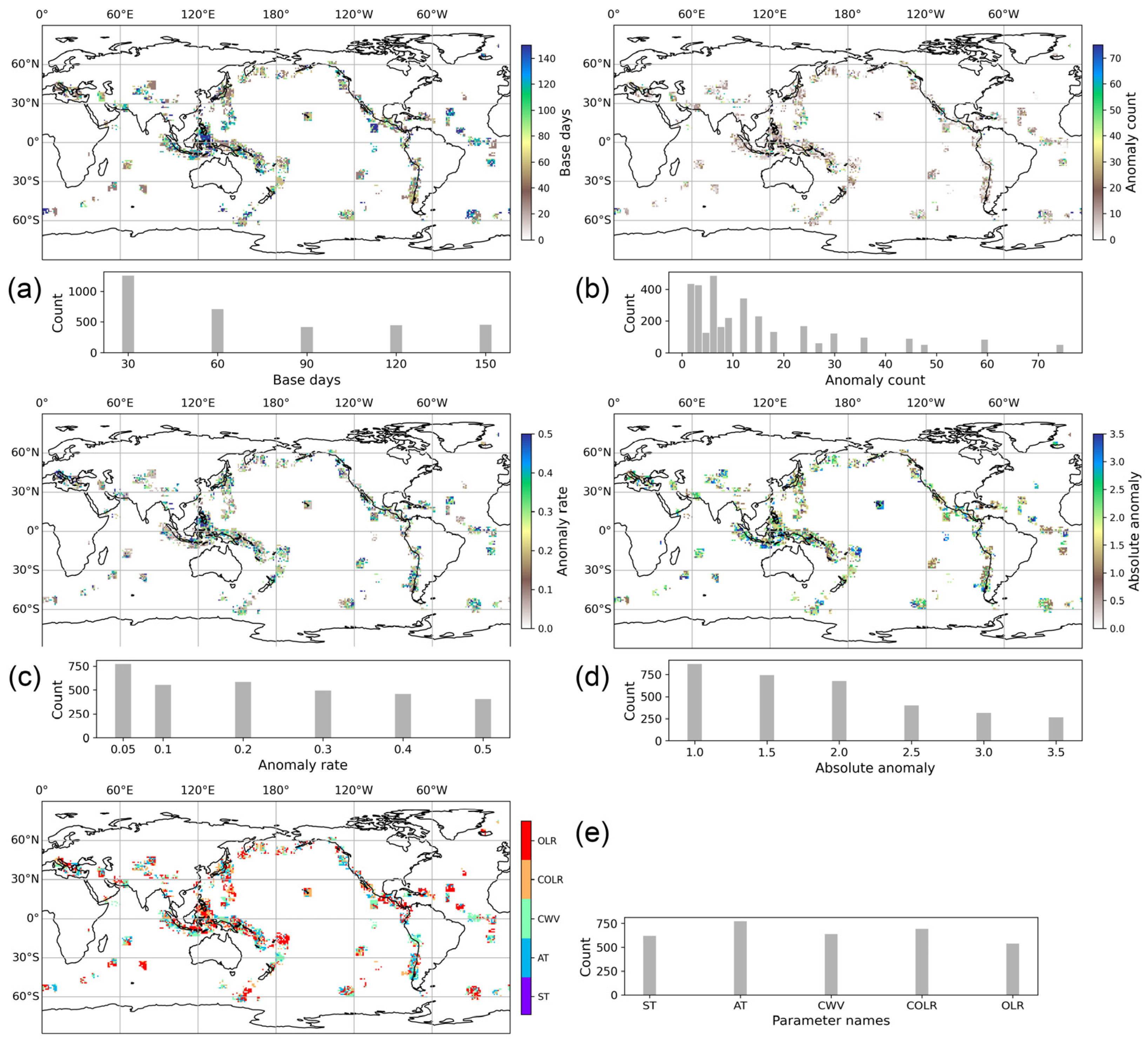
Figure A3.
The optimal parameters for anomaly recognition criteria that are utilized for forecasting impending earthquakes in multiparameter composed anomalies based on training data within 2006–2010, and 2016–2020. These anomalies are analyzed based on their spatial distributions and histograms, as shown in the top and bottom subfigures, respectively. The parameters include (a) the base days preceding earthquakes; (b) the anomaly count that occurred during the base days; (c) the anomaly rate within the spatial window, which is 7 × 7 pixels in this study; (d) the absolute anomaly value used to identify potential earthquake-related anomalies; and (e) the geophysical parameters used in the composed anomalies. ST: skin temperature; AT: air temperature; CWV: total integrated column water vapor burden; OLR: outgoing longwave radiation flux; COLR: clear-sky OLR.

Figure A4.
The optimal parameters for anomaly recognition criteria that are utilized for forecasting impending earthquakes in multiparameter composed anomalies based on training data within 2006–2015. These anomalies are analyzed based on their spatial distributions and histograms, as shown in the top and bottom subfigures, respectively. The parameters include (a) the base days preceding earthquakes; (b) the anomaly count that occurred during the base days; (c) the anomaly rate within the spatial window, which is 7 × 7 pixels in this study; (d) the absolute anomaly value used to identify potential earthquake-related anomalies; and (e) the geophysical parameters used in the composed anomalies. ST: skin temperature; AT: air temperature; CWV: total integrated column water vapor burden; OLR: outgoing longwave radiation flux; COLR: clear-sky OLR.

References
- Marzocchi, W.; Lombardi, A.M.; Casarotti, E. The Establishment of an Operational Earthquake Forecasting System in Italy. Seismol. Res. Lett. 2014, 85, 961–969. [Google Scholar] [CrossRef]
- Huang, Q. Forecasting the epicenter of a future major earthquake. Proc. Natl. Acad. Sci. USA 2015, 112, 944–945. [Google Scholar] [CrossRef]
- Jiao, Z.H.; Shan, X. Short-Term Responses of Land Surface Temperature Anomalies to Earthquakes in China. In Proceedings of the 2021 IEEE International Geoscience and Remote Sensing Symposium IGARSS, Brussels, Belgium, 11–16 July 2021; pp. 8412–8415. [Google Scholar]
- Chen, S.; Liu, P.; Feng, T.; Wang, D.; Jiao, Z.; Chen, L.; Xu, Z.; Zhang, G. Exploring Changes in Land Surface Temperature Possibly Associated with Earthquake: Case of the April 2015 Nepal Mw 7.9 Earthquake. Entropy 2020, 22, 377. [Google Scholar] [CrossRef] [Green Version]
- Khalili, M.; Alavi Panah, S.K.; Abdollahi Eskandar, S.S. Using Robust Satellite Technique (RST) to determine thermal anomalies before a strong earthquake: A case study of the Saravan earthquake (April 16th, 2013, MW = 7.8, Iran). J. Asian Earth Sci. 2019, 173, 70–78. [Google Scholar] [CrossRef]
- Satti, M.S.; Ehsan, M.; Abbas, A.; Shah, M.; de Oliveira-Júnior, J.F.; Naqvi, N.A. Atmospheric and ionospheric precursors associated with M ≥ 6.5 earthquakes from multiple satellites. J. Atmos. Sol.-Terr. Phys. 2022, 227, 105802. [Google Scholar] [CrossRef]
- Shah, M.; Aibar, A.C.; Tariq, M.A.; Ahmed, J.; Ahmed, A. Possible ionosphere and atmosphere precursory analysis related to Mw > 6.0 earthquakes in Japan. Remote Sens. Environ. 2020, 239, 111620. [Google Scholar] [CrossRef]
- Jing, F.; Singh, R.P.; Shen, X. Land–Atmosphere–Meteorological coupling associated with the 2015 Gorkha (M 7.8) and Dolakha (M 7.3) Nepal earthquakes. Geomat. Nat. Hazards Risk 2019, 10, 1267–1284. [Google Scholar] [CrossRef] [Green Version]
- Marchetti, D.; De Santis, A.; Shen, X.; Campuzano, S.A.; Perrone, L.; Piscini, A.; Di Giovambattista, R.; Jin, S.; Ippolito, A.; Cianchini, G.; et al. Possible Lithosphere-Atmosphere-Ionosphere Coupling effects prior to the 2018 Mw = 7.5 Indonesia earthquake from seismic, atmospheric and ionospheric data. J. Asian Earth Sci. 2020, 188, 104097. [Google Scholar] [CrossRef]
- Wu, L.; Zheng, S.; De Santis, A.; Qin, K.; Di Mauro, R.; Liu, S.; Rainone, M.L. Geosphere coupling and hydrothermal anomalies before the 2009 Mw 6.3 L’Aquila earthquake in Italy. Nat. Hazards Earth Syst. Sci. 2016, 16, 1859–1880. [Google Scholar] [CrossRef] [Green Version]
- Sun, K.; Shan, X.; Ouzounov, D.; Shen, X.; Jing, F. Analyzing long wave radiation data associated with the 2015 Nepal earthquakes based on Multi-orbit satellite observations. Chin. J. Geophys. 2017, 60, 3457–3465. [Google Scholar]
- Jordan, T.H.; Chen, Y.-T.; Gasparini, P.; Madariaga, R.; Main, I.; Marzocchi, W.; Papadopoulos, G.; Sobolev, G.; Yamaoka, K.; Zschau, J. Operational earthquake forecasting: State of Knowledge and Guidelines for Utilization. Ann. Geophys. 2011, 54, 316–391. [Google Scholar]
- Kato, A.; Ben-Zion, Y. The generation of large earthquakes. Nat. Rev. Earth Environ. 2020, 2, 26–39. [Google Scholar]
- Molchanov, O.; Fedorov, E.; Schekotov, A.; Gordeev, E.; Chebrov, V.; Surkov, V.; Rozhnoi, A.; Andreevsky, S.; Iudin, D.; Yunga, S.; et al. Lithosphere-atmosphere-ionosphere coupling as governing mechanism for preseismic short-term events in atmosphere and ionosphere. Nat. Hazards Earth Syst. Sci. 2004, 4, 757–767. [Google Scholar] [CrossRef] [Green Version]
- Denisenko, V.V.; Boudjada, M.Y.; Lammer, H. Propagation of Seismogenic Electric Currents Through the Earth’s Atmosphere. J. Geophys. Res. Space Phys. 2018, 123, 4290–4297. [Google Scholar]
- Tramutoli, V.; Aliano, C.; Corrado, R.; Filizzola, C.; Genzano, N.; Lisi, M.; Martinelli, G.; Pergola, N. On the possible origin of thermal infrared radiation (TIR) anomalies in earthquake-prone areas observed using robust satellite techniques (RST). Chem. Geol. 2013, 339, 157–168. [Google Scholar]
- Freund, F.; Ouillon, G.; Scoville, J.; Sornette, D. Earthquake precursors in the light of peroxy defects theory: Critical review of systematic observations. Eur. Phys. J. Spec. Top. 2021, 230, 7–46. [Google Scholar]
- Ren, Y.; Ma, J.; Liu, P.; Chen, S. Experimental Study of Thermal Field Evolution in the Short-Impending Stage Before Earthquakes. Pure Appl. Geophys. 2017, 175, 2527–2539. [Google Scholar] [CrossRef]
- Liu, P.; Chen, S.; Liu, Q.; Guo, Y.; Ren, Y.; Zhuo, Y.; Feng, J. A Potential Mechanism of the Satellite Thermal Infrared Seismic Anomaly Based on Change in Temperature Caused by Stress Variation: Theoretical, Experimental and Field Investigations. Remote Sens. 2022, 14, 5697. [Google Scholar] [CrossRef]
- Jiao, Z.-H.; Shan, X. Statistical framework for the evaluation of earthquake forecasting: A case study based on satellite surface temperature anomalies. J. Asian Earth Sci. 2021, 211, 104710. [Google Scholar] [CrossRef]
- Genzano, N.; Filizzola, C.; Hattori, K.; Pergola, N.; Tramutoli, V. Statistical Correlation Analysis Between Thermal Infrared Anomalies Observed From MTSATs and Large Earthquakes Occurred in Japan (2005–2015). J. Geophys. Res. Solid Earth 2021, 126, e2020JB020108. [Google Scholar]
- Fu, C.-C.; Lee, L.-C.; Ouzounov, D.; Jan, J.-C. Earth’s Outgoing Longwave Radiation Variability Prior to M ≥ 6.0 Earthquakes in the Taiwan Area During 2009–2019. Front. Earth Sci. 2020, 8, 364. [Google Scholar] [CrossRef]
- Eleftheriou, A.; Filizzola, C.; Genzano, N.; Lacava, T.; Lisi, M.; Paciello, R.; Pergola, N.; Vallianatos, F.; Tramutoli, V. Long-term RST analysis of anomalous TIR sequences in relation with earthquakes occurred in Greece in the period 2004–2013. Pure Appl. Geophys. 2016, 173, 285–303. [Google Scholar] [CrossRef] [Green Version]
- Zhang, Y.; Meng, Q. A statistical analysis of TIR anomalies extracted by RSTs in relation to an earthquake in the Sichuan area using MODIS LST data. Nat. Hazards Earth Syst. Sci. 2019, 19, 535–549. [Google Scholar] [CrossRef] [Green Version]
- Jiao, Z.-H.; Shan, X. Consecutive statistical evaluation framework for earthquake forecasting: Evaluating satellite surface temperature anomaly detection methods. J. Asian Earth Sci. X 2022, 7, 100096. [Google Scholar] [CrossRef]
- Picozza, P.; Conti, L.; Sotgiu, A. Looking for Earthquake Precursors From Space: A Critical Review. Front. Earth Sci. 2021, 9, 676775. [Google Scholar] [CrossRef]
- Jiao, Z.-H.; Zhao, J.; Shan, X. Pre-seismic anomalies from optical satellite observations: A review. Nat. Hazards Earth Syst. Sci. 2018, 18, 1013–1036. [Google Scholar] [CrossRef] [Green Version]
- Jenkins, A.P.; Biggs, J.; Rust, A.C.; Rougier, J.C. Decadal Timescale Correlations Between Global Earthquake Activity and Volcanic Eruption Rates. Geophys. Res. Lett. 2021, 48, e2021GL093550. [Google Scholar] [CrossRef]
- Chahine, M.T.; Pagano, T.S.; Aumann, H.H.; Atlas, R.; Barnet, C.; Blaisdell, J.; Chen, L.; Divakarla, M.; Fetzer, E.J.; Goldberg, M.; et al. AIRS: Improving weather forecasting and providing new data on greenhouse gases. Bull. Am. Meteorol. Soc. 2006, 87, 911–926. [Google Scholar] [CrossRef] [Green Version]
- Wu, L.; Qi, Y.; Mao, W.; Lu, J.; Ding, Y.; Peng, B.; Xie, B. Scrutinizing and rooting the multiple anomalies of Nepal earthquake sequence in 2015 with the deviation–time–space criterion and homologous lithosphere–coversphere–atmosphere–ionosphere coupling physics. Nat. Hazards Earth Syst. Sci. 2023, 23, 231–249. [Google Scholar] [CrossRef]
- Chicco, D.; Jurman, G. The advantages of the Matthews correlation coefficient (MCC) over F1 score and accuracy in binary classification evaluation. BMC Genom. 2020, 21, 6. [Google Scholar] [CrossRef] [Green Version]
- Filizzola, C.; Corrado, A.; Genzano, N.; Lisi, M.; Pergola, N.; Colonna, R.; Tramutoli, V. RST Analysis of Anomalous TIR Sequences in Relation with Earthquakes Occurred in Turkey in the Period 2004–2015. Remote Sens. 2022, 14, 381. [Google Scholar] [CrossRef]
- Jiao, Z.; Shan, X. Pre-Seismic Temporal Integrated Anomalies from Multiparametric Remote Sensing Data. Remote Sens. 2022, 14, 2343. [Google Scholar] [CrossRef]
- Pulinets, S.; Ouzounov, D. Lithosphere–Atmosphere–Ionosphere Coupling (LAIC) model—An unified concept for earthquake precursors validation. J. Asian Earth Sci. 2011, 41, 371–382. [Google Scholar] [CrossRef]
- Xiong, P.; Tong, L.; Zhang, K.; Shen, X.; Battiston, R.; Ouzounov, D.; Iuppa, R.; Crookes, D.; Long, C.; Zhou, H. Towards advancing the earthquake forecasting by machine learning of satellite data. Sci. Total Environ. 2021, 771, 145256. [Google Scholar] [CrossRef]
- Genzano, N.; Filizzola, C.; Lisi, M.; Pergola, N.; Tramutoli, V. Toward the development of a multi parametric system for a short-term assessment of the seismic hazard in Italy. Ann. Geophys. 2020, 63, 550. [Google Scholar] [CrossRef]
- Freund, F. Toward a unified solid state theory for pre-earthquake signals. Acta Geophys. 2010, 58, 719. [Google Scholar] [CrossRef]
- Quigley, M.C.; Hughes, M.W.; Bradley, B.A.; van Ballegooy, S.; Reid, C.; Morgenroth, J.; Horton, T.; Duffy, B.; Pettinga, J.R. The 2010–2011 Canterbury Earthquake Sequence: Environmental effects, seismic triggering thresholds and geologic legacy. Tectonophysics 2016, 672–673, 228–274. [Google Scholar] [CrossRef] [Green Version]
- Han, Y.; Zang, Y.; Meng, L.; Wang, Y.; Deng, S.; Ma, Y.; Xie, M. A summary of seismic activities in and around China in 2021. Earthq. Res. Adv. 2022, 2, 100157. [Google Scholar] [CrossRef]
- Xu, X.; Chen, S.; Zhang, S.; Dai, R. Analysis of Potential Precursory Pattern at Earth Surface and the Above Atmosphere and Ionosphere Preceding Two Mw ≥ 7 Earthquakes in Mexico in 2020–2021. Earth Space Sci. 2022, 9, e2022EA002267. [Google Scholar] [CrossRef]
- Reichstein, M.; Camps-Valls, G.; Stevens, B.; Jung, M.; Denzler, J.; Carvalhais, N.; Prabhat, F. Deep learning and process understanding for data-driven Earth system science. Nature 2019, 566, 195–204. [Google Scholar] [CrossRef]
- Hardebeck, J.L. Spatial Clustering of Aftershocks Impacts the Performance of Physics-Based Earthquake Forecasting Models. J. Geophys. Res. Solid Earth 2021, 126, e2020JB020824. [Google Scholar] [CrossRef]
- Rundle, J.B.; Stein, S.; Donnellan, A.; Turcotte, D.L.; Klein, W.; Saylor, C. The complex dynamics of earthquake fault systems: New approaches to forecasting and nowcasting of earthquakes. Rep. Prog. Phys. 2021, 84, 076801. [Google Scholar] [CrossRef] [PubMed]
Figure 1.
A total of 1825 global earthquakes with magnitudes ≥ 6 and focal depths ≤ 70 km, that occurred between 2006 and 2020, from the United States Geological Survey (USGS) Earthquake Hazards Program catalog. (a) Earthquake locations depicted as red dots. The altitude data used are sourced from the ETOPO Global Relief Model 2022, available at https://www.ncei.noaa.gov/products/etopo-global-relief-model (accessed on 28 July 2023). (b) Earthquake magnitudes varied with time.

Figure 2.
The optimal parameters of the anomaly recognition criteria employed for forecasting imminent earthquakes using the outgoing longwave radiation anomaly based on training data within 2011–2020, as indicated by their spatial distributions and histograms in the top and bottom subfigures, respectively. The parameters include (a) the base days preceding earthquakes; (b) the anomaly count that occurred during the base days; (c) the anomaly rate within the spatial window, which is 7 × 7 pixels in this study; and (d) the absolute anomaly value used to identify potential earthquake-related anomalies.

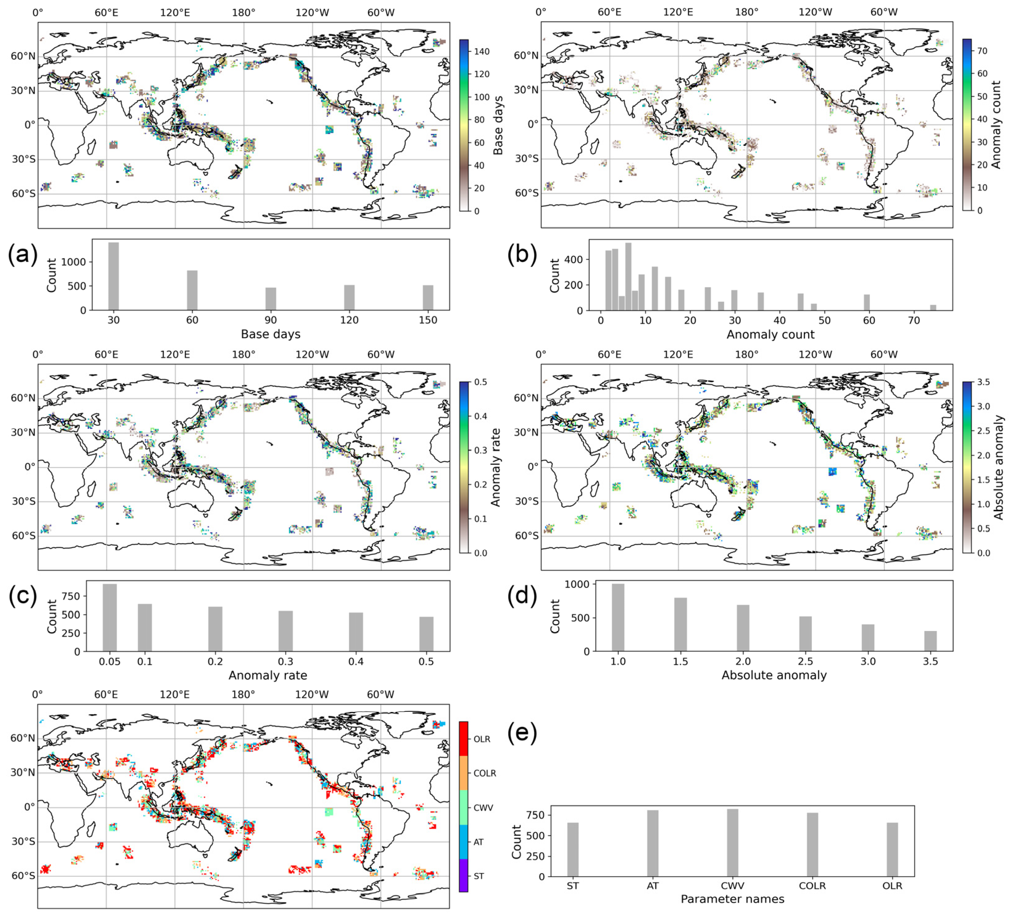
Figure 3.
The optimal parameters for anomaly recognition criteria that are utilized for forecasting impending earthquakes in multiparameter composed anomalies based on training data within 2011–2020. These anomalies are analyzed based on their spatial distributions and histograms, as shown in the top and bottom subfigures, respectively. The parameters include (a) the base days preceding earthquakes; (b) the anomaly count that occurred during the base days; (c) the anomaly rate within the spatial window, which is 7 × 7 pixels in this study; (d) the absolute anomaly value used to identify potential earthquake-related anomalies; and (e) the geophysical parameters used in the composed anomalies. ST: skin temperature; AT: air temperature; CWV: total integrated column water vapor burden; OLR: outgoing longwave radiation flux; COLR: clear-sky OLR.

Figure 4.
The spatial distributions and histograms of Matthew’s correlation coefficients (MCC) obtained using the optimal parameters of anomaly recognition criteria at the training stage based on training data within 2011–2020 for (a) skin temperature (ST), (b) air temperature (AT), (c) clear-sky outgoing longwave radiation (COLR), (d) outgoing longwave radiation (OLR), and (e) total integrated column water vapor burden (CWV) anomalies.

Figure 5.
The spatial distributions and histograms of Matthew’s correlation coefficients (MCC) obtained using the optimal parameters of anomaly recognition criteria at the test stage for 2006–2010, based on training data within 2011–2020 for (a) skin temperature (ST), (b) air temperature (AT), (c) clear-sky outgoing longwave radiation (COLR), (d) outgoing longwave radiation (OLR), (e) total integrated column water vapor burden (CWV), and (f) composed (COM) anomalies.

Figure 6.
The spatial distributions and histograms of Matthew’s correlation coefficients (MCC) when using a single set of anomaly recognition criterion for (a) skin temperature (ST), (b) air temperature (AT), (c) clear-sky outgoing longwave radiation (COLR), (d) outgoing longwave radiation (OLR), and (e) total integrated column water vapor burden (CWV) anomalies within 2006–2010. The temporal range for predicting impending earthquakes was 120 days. The pixel with absolute anomaly value of ≥2 is considered as a valid anomaly pixel. Within the sliding window, the number of valid anomaly pixels is ≥10%. Within the observation period (i.e., 120 days), if there are ≥12 days that satisfy the above conditions, a pre-seismic anomaly is identified.

Figure 7.
Histograms of Matthew’s correlation coefficients (MCC), which were obtained for (a) inland, (b) oceanic, and (c) coastal earthquakes (EQ) for five geophysical and composed parameters. They were computed using the optimal parameters of anomaly recognition. The dash line denotes the MCC of 0.1. ST: skin temperature; AT: air temperature; CWV: total integrated column water vapor burden; OLR: outgoing longwave radiation flux; COLR: clear-sky OLR; COM: composed anomalies.

Figure 8.
The spatial distributions and histograms (top and bottom sub-figures, respectively) of Matthew’s correlation coefficients (MCC) of five geophysical and composed (COM) parameters in China and the surrounding region. ST: skin temperature; AT: air temperature; CWV: total integrated column water vapor burden; OLR: outgoing longwave radiation flux; COLR: clear-sky OLR.

Figure 9.
A statistical evaluation framework for earthquake forecasting.


Table 1.
The time division for the 3-fold cross-validation implemented to acquire the optimal anomaly identification parameters for each geophysical parameter.
Table 1.
The time division for the 3-fold cross-validation implemented to acquire the optimal anomaly identification parameters for each geophysical parameter.
| No. | Years for Training Data | Years for Test Data |
|---|---|---|
| 1 | 2011–2020 | 2006–2010 |
| 2 | 2006–2010, and 2016–2020 | 2011–2015 |
| 3 | 2006–2015 | 2016–2020 |
Table 2.
The statistical results of the Matthew’s correlation coefficient (MCC) conducted for earthquake forecasting utilizing anomalies derived from selected geophysical parameters. The seismically active region, as depicted in Figure 4 of [25], encompasses a total of 12,034 pixels. The ratio refers to the number of valid anomaly pixels divided by the aforementioned total count. ST: skin temperature; AT: air temperature; CWV: total integrated column water vapor burden; OLR: outgoing longwave radiation flux; COLR: clear-sky OLR; COM: composed anomalies.
| Stage | Training | Test | ||||||
|---|---|---|---|---|---|---|---|---|
| Parameter | Min | Max | Mean | Ratio | Min | Max | Mean | Ratio |
| ST | 0.008 | 1 | 0.272 | 0.836 | 0.001 | 1 | 0.122 | 0.200 |
| AT | 0.029 | 1 | 0.299 | 0.836 | 0.002 | 1 | 0.150 | 0.170 |
| CWV | 0.024 | 1 | 0.305 | 0.836 | 0.002 | 1 | 0.145 | 0.165 |
| COLR | 0.024 | 1 | 0.303 | 0.836 | 0.002 | 1 | 0.150 | 0.174 |
| OLR | 0.034 | 1 | 0.338 | 0.836 | 0.002 | 0.701 | 0.152 | 0.164 |
| COM | / | / | / | / | 0.002 | 1 | 0.186 | 0.424 |
Table 3.
The statistical results of the Matthew’s correlation coefficient (MCC) for inland, oceanic, and coastal earthquakes (EQ). ST: skin temperature; AT: air temperature; CWV: total integrated column water vapor burden; OLR: outgoing longwave radiation flux; COLR: clear-sky OLR; COM: composed anomalies.
| Type | Parameter | Min | Max | Mean |
|---|---|---|---|---|
| Inland EQ | ST | 0.002 | 0.567 | 0.118 |
| AT | 0.002 | 0.567 | 0.149 | |
| CWV | 0.002 | 0.649 | 0.139 | |
| COLR | 0.004 | 0.695 | 0.140 | |
| OLR | 0.002 | 0.487 | 0.152 | |
| COM | 0.002 | 0.695 | 0.176 | |
| Oceanic EQ | ST | 0.001 | 1.000 | 0.124 |
| AT | 0.002 | 1.000 | 0.153 | |
| CWV | 0.002 | 1.000 | 0.149 | |
| COLR | 0.002 | 1.000 | 0.157 | |
| OLR | 0.002 | 0.701 | 0.150 | |
| COM | 0.002 | 1.000 | 0.189 | |
| Coastal EQ | ST | 0.002 | 0.701 | 0.116 |
| AT | 0.002 | 0.701 | 0.142 | |
| CWV | 0.002 | 0.701 | 0.137 | |
| COLR | 0.002 | 1.000 | 0.136 | |
| OLR | 0.003 | 0.701 | 0.157 | |
| COM | 0.002 | 1.000 | 0.183 |
Disclaimer/Publisher’s Note: The statements, opinions and data contained in all publications are solely those of the individual author(s) and contributor(s) and not of MDPI and/or the editor(s). MDPI and/or the editor(s) disclaim responsibility for any injury to people or property resulting from any ideas, methods, instructions or products referred to in the content. |
© 2023 by the authors. Licensee MDPI, Basel, Switzerland. This article is an open access article distributed under the terms and conditions of the Creative Commons Attribution (CC BY) license (https://creativecommons.org/licenses/by/4.0/).
Share and Cite
MDPI and ACS Style
Jiao, Z.; Hao, Y.; Shan, X. A Spatially Self-Adaptive Multiparametric Anomaly Identification Scheme Based on Global Strong Earthquakes. Remote Sens. 2023, 15, 3803. https://doi.org/10.3390/rs15153803
AMA Style
Jiao Z, Hao Y, Shan X. A Spatially Self-Adaptive Multiparametric Anomaly Identification Scheme Based on Global Strong Earthquakes. Remote Sensing. 2023; 15(15):3803. https://doi.org/10.3390/rs15153803
Chicago/Turabian StyleJiao, Zhonghu, Yumeng Hao, and Xinjian Shan. 2023. "A Spatially Self-Adaptive Multiparametric Anomaly Identification Scheme Based on Global Strong Earthquakes" Remote Sensing 15, no. 15: 3803. https://doi.org/10.3390/rs15153803
Note that from the first issue of 2016, this journal uses article numbers instead of page numbers. See further details here.