
A Model for Estimating the Earth’s Outgoing Radiative Flux from A Moon-Based Radiometer

1
Key Laboratory of Thermo-Fluid Science and Engineering, Ministry of Education, School of Energy and Power Engineering, Xi’an Jiaotong University, Xi’an 710049, China
2
Royal Observatory of Belgium, Avenue Circulaire 3, 1180 Brussels, Belgium
*
Author to whom correspondence should be addressed.
Remote Sens. 2023, 15(15), 3773; https://doi.org/10.3390/rs15153773
Submission received: 2 June 2023
/
Revised: 26 July 2023
/
Accepted: 28 July 2023
/
Published: 29 July 2023
(This article belongs to the Special Issue Earth Radiation Budget and Earth Energy Imbalance)
Abstract
:A Moon-based radiometer can provide continuous measurements for the Earth’s full-disk broadband irradiance, which is useful for studying the Earth’s Radiation Budget (ERB) at the height of the Top of the Atmosphere (TOA). The ERB describes how the Earth obtains solar energy and emits energy to space through the outgoing broadband Short-Wave (SW) and emitted thermal Long-Wave (LW) radiation. In this work, a model for estimating the Earth’s outgoing radiative flux from the measurements of a Moon-based radiometer is established. Using the model, the full-disk LW and SW outgoing radiative flux are gained by converting the unfiltered entrance pupil irradiances (EPIs) with the help of the anisotropic characteristics of the radiances. Based on the radiative transfer equation, the unfiltered EPI time series is used to validate the established model. By comparing the simulations for a Moon-based radiometer with the satellite-based data from the National Institute of Standards and Technology Advanced Radiometer (NISTAR) and the Clouds and the Earth’s Radiant Energy System (CERES) datasets, the simulations show that the daytime SW fluxes from the Moon-based measurements are expected to vary between 194 and 205 Wm−2; these simulations agree well with the CERES data. The simulations are about 5 to 20 Wm−2 smaller than the NISTAR data. For the simulated Moon-based LW fluxes, the range is 251~287 Wm−2. The Moon-based and NISTAR fluxes are consistently 5~15 Wm−2 greater than CERES LW fluxes, and both of them also show larger diurnal variations compared with the CERES fluxes. The correlation coefficients of SW fluxes for Moon-based data and NISTAR data are 0.97, 0.63, and 0.53 for the months of July, August, and September, respectively. Compared with the SW flux, the correlation of LW fluxes is more stable for the same period and the correlation coefficients are 0.87, 0.69, and 0.61 for July to September 2017.
1. Introduction
The climate change of the Earth atmosphere system is measured by the Earth Radiation Budget (ERB) at the height of Earth’s Top of the Atmosphere (TOA). The ERB describes how the Earth obtains solar energy and emits energy to space through Outgoing Short-Wave (SW) Radiation (OSR) in the spectral range of 0.2–5 μm and Long-Wave (LW) Radiation (OLR) in the spectral range from 5 to 200 μm. The long-term and stable monitoring of the ERB is important for understanding the Earth’s climate system and its evolution timely [1,2,3,4,5]. For the study of the ERB, satellite observation data provide critical information for understanding the driving mechanisms of climate change. Monitoring the ERB from space begins with the early satellite missions of the 1960s, such as NASA’s Explorer 7 [6], and afterward, many dedicated ERB satellite instruments were launched to obtain the OLR and OSR, such as the Earth Radiation Budget Experiment (ERBE) [7], the Clouds and the Earth’s Radiant Energy System (CERES) [8,9], the Geostationary Earth Radiation Budget (GERB) [3,4], and the Deep Space Climate Observatory (DSCOVR) [10]. Although the observation data from the satellite-based sensors have improved our understanding of the ERB [11,12], there still exists several limitations for satellite observation, such as limited lifetime, limited instantaneous field of view, and limited temporal sampling [2,3,4,5,6,7,10,13,14,15].
As the Earth’s only natural satellite, a special platform that is different from the artificial satellites, the nearside of the Moon shows great potential for performing Earth’s outgoing radiation observation. A Moon-based Wide Field-of-View Radiometer (MWFVR) can provide full-disk broadband irradiance measurements at a planetary hemispherical scale, which will augment and enrich the ERB data products. The MWFVR can observe nearly half of the Earth due to the large Earth–Moon distance [16,17]. The Moon’s orbit is close to an ellipse with an eccentricity of 0.0549 and the inclination angle between the orbital plane and the ecliptic plane is about 5.15°. The huge nearside of the Moon facing the Earth also provides plenty of locations for setting the various types of sensors to obtain scientific data, such as cloud fraction and aerosol optical depth. In addition, the long lifetime and stable orbit of the Moon can provide continuous high-frequency Earth observations, which help to enrich the record covering all local times and all seasons in a year. Of course, the special working environment also brings some new challenges to the Moon-based Earth radiation observation instrument, such as the large temperature change between day and nighttime (~300 K) [18], the high-energy particles from outer space, and Moon dust. Fortunately, similar situations and challenges also appear for satellite observation, lunar landers, and rovers, and many technologies have been invented and applied to overcome these challenges [14,15,16,17,18]. The successful design experience with the Extreme Ultra-Violet Camera, a scientific payload onboard the lander of the Chang’E-3 mission, has been demonstrated as achievable with existing technology [18].
Until now, several studies have been conducted considering the Moon as a platform for Earth observations and the work mainly focuses on the feasibility and effectiveness of the method [17,19,20], geometric model simulations [18,19,20,21,22], and the potential applications and ascertainment of a sampling scheme [23,24,25,26]. The determination of the Earth’s energy imbalance (EEI) of the Earth atmosphere needs the outgoing SW and LW radiative fluxes (OSR and OLR), so developing the estimating model of Earth’s outgoing radiative flux from the measurements of the MWFVR is a key step. The objective of this work is to develop and build a model to obtain the Earth’s outgoing radiative flux from the MWFVR’s measurements based on the correction factors and the Global Mean Anisotropic Factors (GMAFs). Section 2 is dedicated to presenting the observation geometry, the construction process of the model framework, and the methodology. In Section 3, all of the results and a discussion are presented in detail. Our conclusions and summaries are presented in Section 4.
2. Model and Methodology
2.1. Observation Geometry
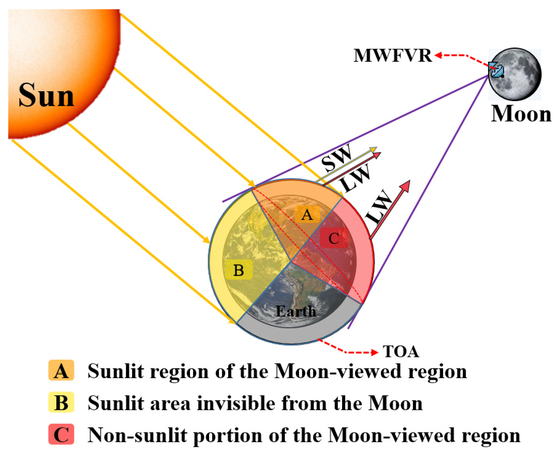
Due to the orbit characteristics of the Moon being different from the Low Earth Orbit (LEO) satellites and the Geostationary Earth Orbit (GEO) satellites, such as the large distance between the Moon and the Earth (3.6 × 10⁵~4.1 × 10⁵ km), it is not appropriate to detect the Earth’s outgoing radiation by a scanning method. Similar to the National Institute of Standards and Technology Advanced Radiometer (NISTAR) onboard the Deep Space Climate Observatory (DSCOVR) [10], placing a dedicated non-scanning Moon-based Wide Field-of-View Radiometer (MWFVR) on the lunar nearside is suitable, which means that Earth’s outgoing radiation from the Top of the Atmosphere (TOA) can be monitored by observing the Earth as a one-pixel radiative source [27]. Moreover, the time interpolation error caused by orbit limitations can also be mitigated by the high-frequency temporal samples of the wide field-of-view observations. Therefore, firstly, it is necessary to build a new observation geometric model for the MWFVR. Figure 1 shows the observation geometry of the MWFVR. The sunlit and MWFVR-viewed regions are shown in different colors and indicated by the symbols, A, B, and C. The light-red sector represents the visible regions of the MWFVR at the Earth’s TOA (region A plus region C) and the light-yellow sector represents the sunlit area (region A plus region B). The nearly hemispherical instantaneous field of view of the MWFVR consists of bright areas (region A) and dark regions (region C). The bright part emits not only the Outgoing LW radiation (5–200 μm) (OLR) but also the Outgoing SW Radiation (0.2–5 μm) (OSR) reflected by the Earth atmosphere system. The dark area emits only the OLR. Because the Moon always faces Earth with the same side—the so-called nearside—and the Earth’s rotation period is 24 h, the MWFVR can sample and observe the whole surface of the Earth in one day [20,21]. In addition, due to the inclination angle between the Moon’s orbital plane with the ecliptic plane being about 5.15°, the MWFVR-viewed region at Earth’s TOA varies with time. The sunlit part is also a temporal variable. In addition, the curvature of the Earth’s hemispheric surface in the MWFVR’s instantaneous field of view will result in spatial variations [20,21] of the contributions of different Earth’s sites to the MWFVR’s SW and LW Entrance Pupil Irradiance (EPI).
2.2. Radiation Transfer Function
Irradiance is the energy that reaches the entrance pupil plane of the MWFVR, and finally, it arrives at the detection element. Afterward, the incident radiative energy is converted to a digital signal and stored by the data acquisition system. The instantaneous EPI, ΦSW/LW, measured by the MWFVR, at a lunar location (latitude θMoon and longitude λMoon), is a triple integral function of the Earth’s outgoing radiation from all positions within the MWFVR-viewed regions [21], as shown in Equations (1) and (2). Although the method of achieving the conversion between radiance and irradiance has evolved over time, the general method remains the same [5]. The Moon-based radiometer’s SW EPI (ΦSW) and LW EPI (ΦLW) which are related to radiance L can be derived from Equations (1) and (2) by using the method of numerical integration. To derive the MWFVR’s EPI of ΦSW and ΦLW, the temporal-spatial distribution of the MWFVR-viewed regions and the sunlit portion at the Earth’s TOA must be first derived. Then, the numerical integration method is utilized by discretizing the MWFVR-viewed region and the sunlit portion into various elements and grids, as shown in Figure 2. The rationale behind the numerical integration method is to sum the individual contributions of each discrete grid node or region in the MWFVR observation regions. The discrete summation equations are expressed as Equations (3) and (4):
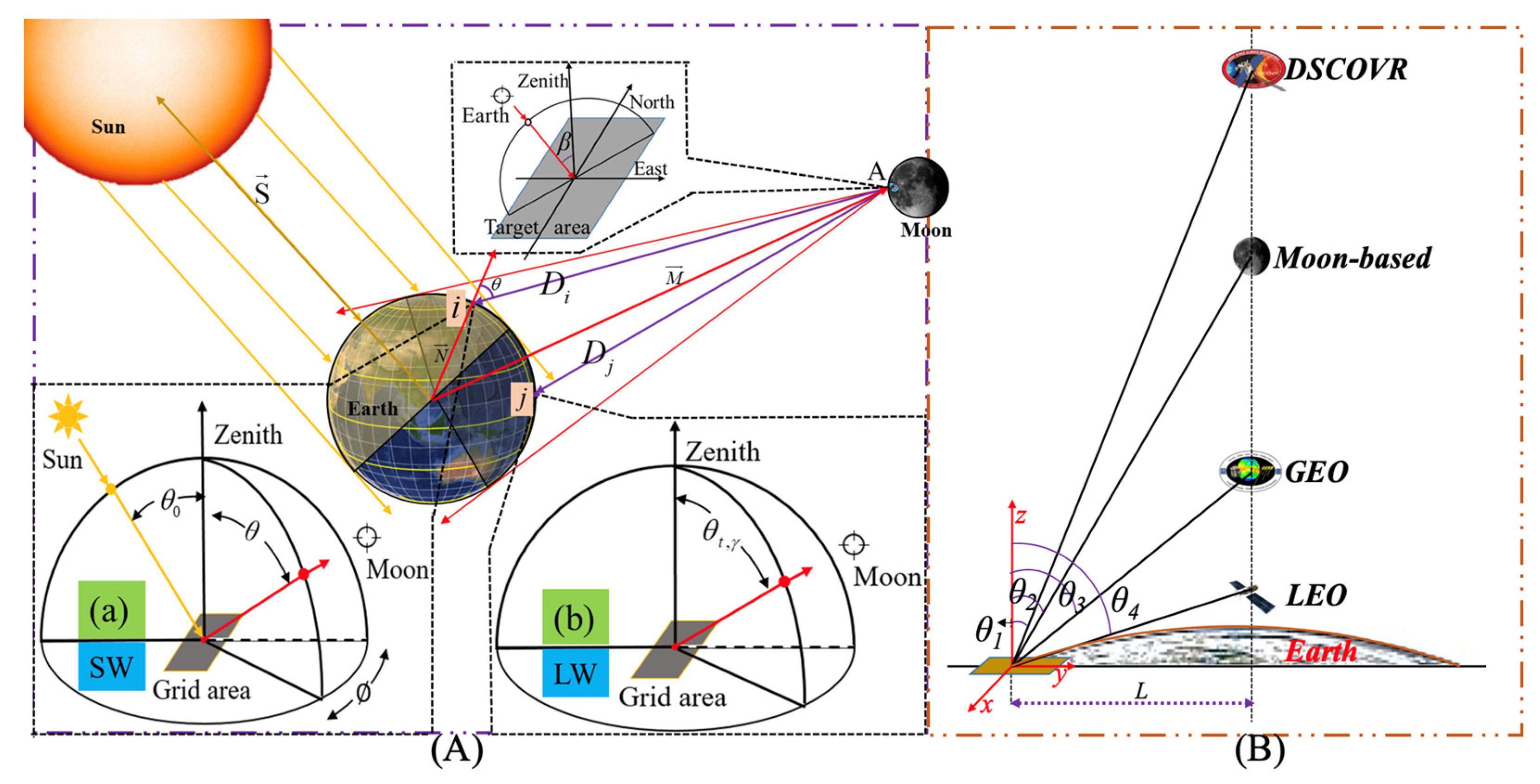
where LSW and LLW are the SW and LW radiances. θ0, θ, and ϕ are the solar zenith angle (SZA), viewing zenith angle (VZA), and relative azimuth angle (RAA) (see Figure 2A). γ and t are the colatitude and the time. Di is the distance between the lunar site of the MWFVR and the discrete grid node i at the Earth’s TOA. βi is the VZA responding to the radiometer’s entrance pupil plane, as shown at the top of Figure 2A. N is the number of discrete grid nodes. For the convenience of calculation, the discrete grid resolution is set to be equal to that of the CERES synthetic datasets, that is, the spatial resolution of Earth’s TOA is 1° latitude × 1° longitude. In the following analysis, for a clearer description, the maximum viewing zenith angle of θmax is called the limit angle and the range is 0~90°.
For a specific satellite platform, such as the LEO satellite carrying a CERES instrument, the contribution of each discrete grid to the EPI can be determined from the TOA radiative fluxes and the angular distribution models (ADMs). In this work, the Clouds and the Earth’s Radiant Energy System (CERES) SYN1deg-1hourly Ed4A product and the Earth Radiation Budget Experiment (ERBE) anisotropic factors [28,29,30] are utilized to solve Equations (3) and (4). The CERES SYN1deg-1Hour Ed4A (https://asdc.larc.nasa.gov/data/CERES/SYN1deg-1Hour/, accessed on 6 September 2021) products (abbreviated as CERES SYN1deg) are the highest temporal resolution TOA flux datasets currently available and the ERBE ADMs are also currently the only complete datasets available. However, because the upwelling radiance cannot instantaneously be measured from any direction, the accurate irradiance in Equations (1)–(4) cannot be derived. Because the angular distribution of outgoing LW and SW radiation can vary with the scene types in the MWFVR-viewed regions, such as land and ocean, the conversion of the directional radiance to the integrated quantity of irradiance is non-trivial. Therefore, a model for this conversion is needed, and such models are referred to as angular distribution models—ADMs—which provide the anisotropic factors. In addition, Figure 2A shows the angular coordinate system for the definition of ERBE ADMs.
In essence, the ADMs are a discretized form of the anisotropic function RLW or RSW and are a set of anisotropic factors, as shown in Equations (5) and (6) [29,30,31,32]. Each ADM is sorted into discrete angular bins and parameters from large radiance measurements for defining an angular distribution model scene type, as shown in Table 1 [33]. The first column is the sequence of the scene number and the fourth column is the sequence number of the angle range number of the viewing zenith angle defined in ERBE ADMs [33,34]. Finally, the mathematical function of RSW/LW that defines ADMs can be expressed as:
where M (θ0) is the SW equivalent Lambertian flux at solar zenith angle θ0. The M (γ, t) is LW equivalent Lambertian flux at colatitude γ and the time t of the year [31]. Different from the RSW, the RLW considers the time variation and it divides the time of the year into 4 seasons [31].
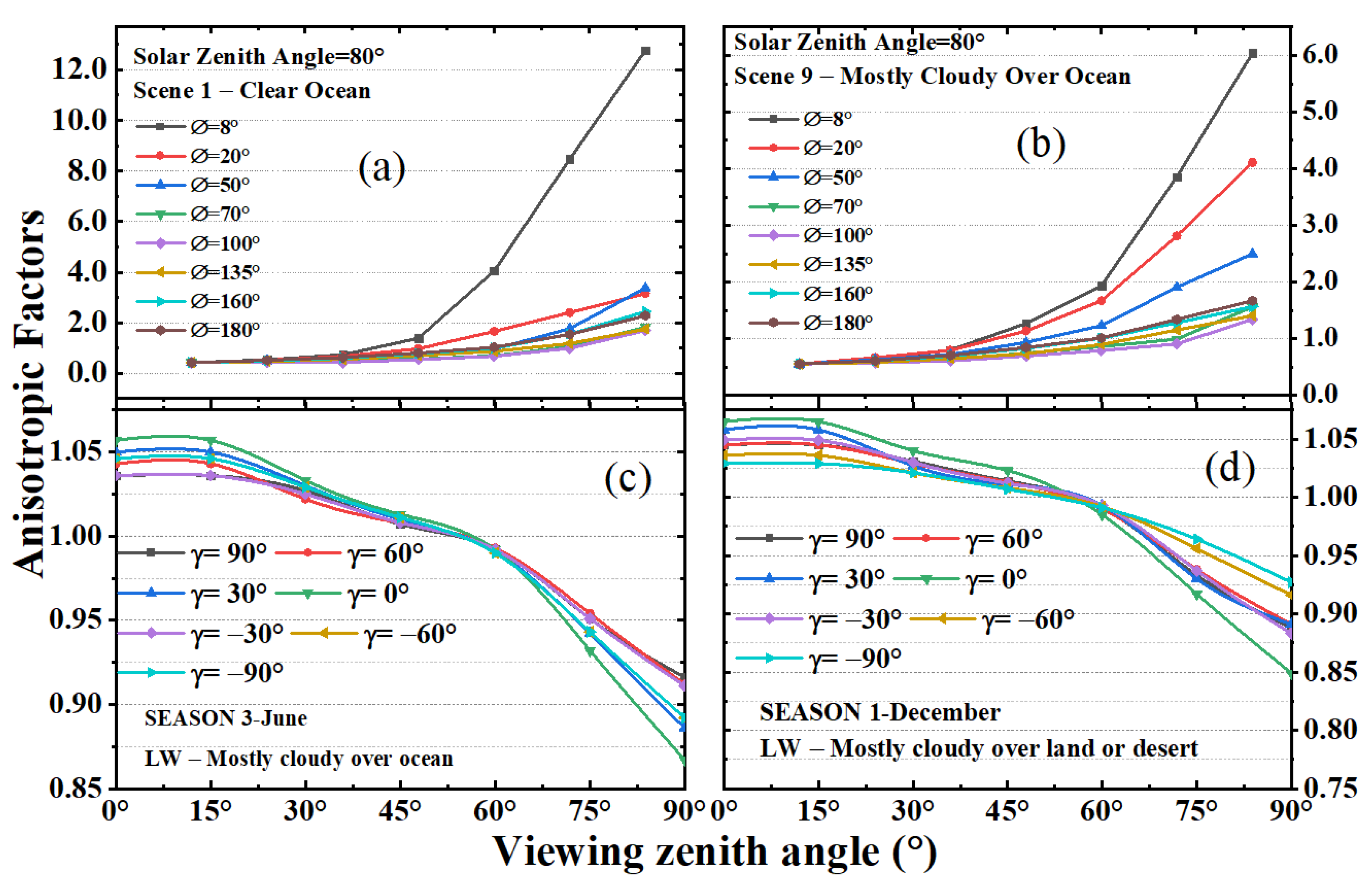
The ADMs are used to achieve the conversion of the radiance to the radiative flux, or irradiance [21], as shown in Equations (5) and (6); in our work, directional radiance is obtained by using the ADMs and CERES TOA fluxes. As the platform height increases, the viewing zenith angle, VZA, will decrease and the corresponding anisotropic factors in the calculation will change. Moreover, the field of view of the radiometer and the effect of Earth’s curvature on the ADMs will both become larger when the height of platforms increases. As shown in Figure 2B, there will be different observation features at distinct platform heights for a given scene and it reveals the relationship between the platform’s height and the angle θ. The SW and LW anisotropic factors from the ERBE ADMs for the different scene types are presented in Figure 3. The X-axis is the angle θ, the Y-axis is the anisotropic factor, and the different colors represent different relative azimuth angles. The trends of the SW anisotropic factors RSW for the different scenes, ‘clear ocean’ and ‘mostly cloudy over the ocean’, are different and RSW will increase with the increase in the angle θ. Due to the change in the geometric relationship, the variation of the relative azimuth angle has a strong influence on the SW anisotropic factors (Figure 3a,b). Compared with RSW, the RLW has a small range of change and will decrease as the angle θ increases. The trend of change for RLW is consistent for different seasons and it reveals that temporal variation has less influence on RLW.
2.3. The Earth’s Outgoing Radiative Flux Estimating Model
Equations (3)–(6) reveal that the ADMs play an important role in the calculation of SW and LW EPIs for a Moon-based radiometer and the results in Figure 3 show that the VZA has a strong influence on ADMs. To compare the difference under two conditions of anisotropy and isotropy in Moon-based Earth radiation observation, we propose to use the anisotropy ratio, Rani, as defined by Equation (7). Rani is the ratio of SW/LW—which represents SW/LW EPIs under isotropic conditions—and ϕSW/LW—which refers to the SW/LW EPIs under anisotropic conditions. The ratio Rani can not only reflect the effect of ADMs on SW and LW EPIs but also indirectly provide constraints for the processing of lunar-based data, as shown in Section 3. Therefore, in this work, we use the ratio Rani to evaluate the influence of anisotropy and it is expressed as:
To determine the Global Mean Anisotropic Factors (GMAFs), we use ERBE ADMs selected based on the scene type information provided by the CERES datasets for every calculated time and the geometrical relationship. So, for a given time, the anisotropic factor for every node i in the radiometer-view region can be determined based on viewing geometry and the ERBE ADMs, and then the GMAFs can be calculated. To effectively utilize Moon-based radiometer detection data, we use the global mean anisotropic factor method to achieve the conversion process from irradiance to radiative flux. The global SW and LW mean radiance in the lunar direction are expressed as:
To obtain the global mean outgoing radiative flux, we use the outgoing grid SW/LW radiative flux from the CERES datasets for each radiometer-viewed region. Finally, the global outgoing mean radiative flux is expressed as:
Finally, the GMAFs, and , are calculated as:
Then, the and can be used to finish the conversion between the Moon-based SW and LW unfiltered radiance, LSW/LW, and the radiative flux:
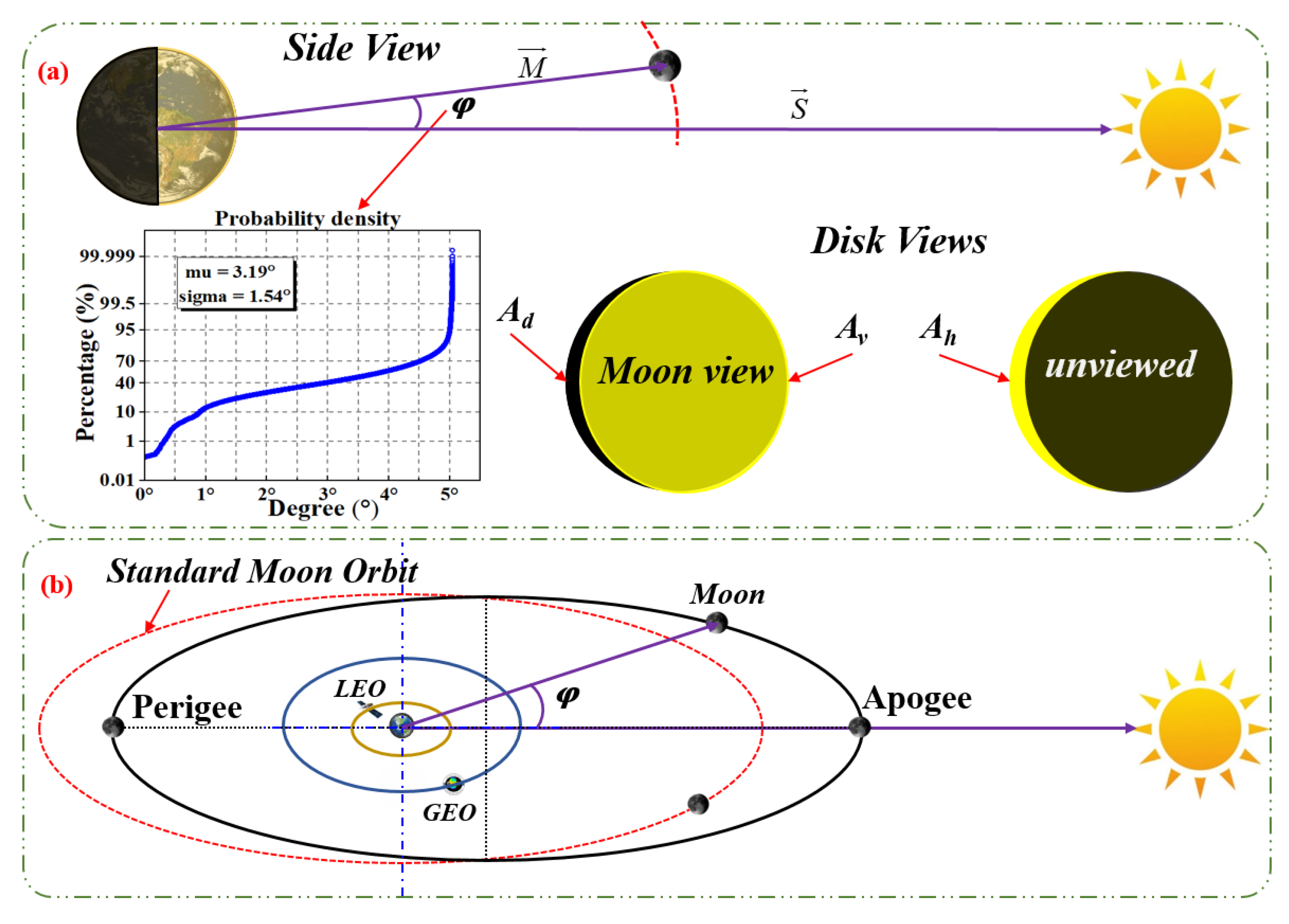
The Moon–Earth distance is a temporal variable and the sunlit portion viewed by the Moon-based radiometer varies with time; therefore, the radiometer-viewed sunlit region is only a part of the sunlit area, as shown in Figure 4a. We refer to the daytime portion that is visible to the MWFVR as (Av) and to the daytime portion that is not visible to the MWFVR as (Ah). The measurements from the MWFVR are not truly “global” daytime measurements. An area correction factor (Av/(Av + Ah)) is introduced to make up for the missing parts (Ah). In general, the angle between the Sun vector and the Moon vector, ϕ, varies from 0° to 180°. The area correction factor is close to one, when the angle ϕ is a small value. The statistics of the smallest time-varying angle, ϕ, are shown in Figure 4a and the range is 0~5.05°. Therefore, the SW daytime outgoing radiative fluxes are calculated only for the period that the angle ϕ is less than 6° and further analysis is shown in Section 3.1. To use the Moon-based measurements to calculate the SW daytime and LW daytime/nighttime Earth outgoing radiative flux and establish a set of standard Moon-based data processing procedures, the correction factor is introduced in Equation (13), and the expression of correction factor KSW/LW is shown in Equation (15). According to the differences of the calculated band, SW or LW, the different expressions are selected in Equation (15). The Moon–Earth orbit is illustrated in Figure 4b. The Moon–Earth distance varies approximately from 3.5 × 10⁵ to 4.1 × 10⁵ km, so we use the average distance of 383,275 km as the standard value to define a standard correction and the establishment of standard data processing procedures as shown in Figure 5.
Equation (15) shows the expression of the whole correction factor. is the ratio of the area () of the sunlit portion at Earth’s TOA to the area () of the radiometer-viewed region, and that is the ratio of the Ad + Av to the Av. The / and the / are the ratios of time-varying distances and time-varying areas to those corresponding values at the mean distance moment, respectively. Using Equations (3)–(6), we can obtain the MWFVR’s EPI, which is the unfiltered energy with the unit of W·m−2. Therefore, we need to use transformation Equation (14) to finish the conversion procession from irradiance (unit: Wm−2) to radiance (unit: Wm−2sr−1).
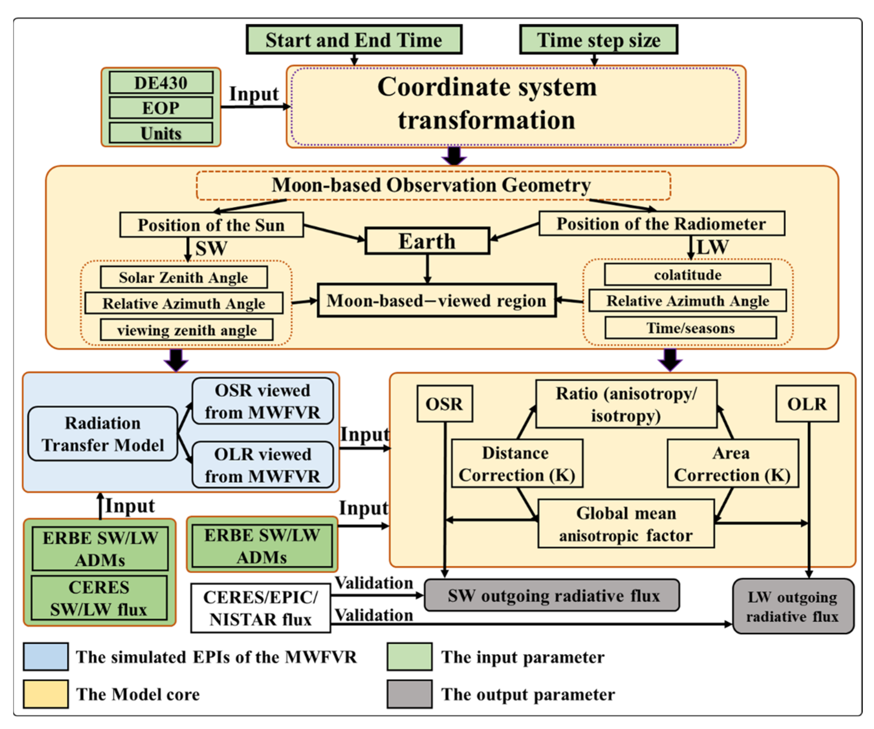
The established model framework for estimating the Earth’s outgoing radiative flux based on the measurements of the MWFVR is shown in Figure 5.
- (1)
- The input parameter: We build the temporal system and spatial coordinate system transformation by using the Planetary and Lunar Ephemerides DE430 and Earth orientation parameters (EOP) [35,36]. The time system is the Coordinated Universal Time (UTC) in this work and a linear transformation can be conducted between different systems. The unification of the spatial coordinate system involves five basic coordinate systems, and the transformation of coordinate systems is completed by a series of matrix operations. The more detailed coordinate transformation can be found in Refs. [20,37]. The start time, end time, and time step are used to determine the exact spatial geometry. Based on the observation geometry, the precise position relationship can be gained, which is the key step in ascertaining the radiometer-viewed region and sunlit area. Here, by calculating the zenith angle of the Moon and the Sun for each global observation grid, we mark all grids where the zenith angle is larger than zero degrees as “1” and the rest as “0” to map out these regions. Then, based on the grid visibility, the established model is used to obtain the Earth’s outward radiative heat flow.
- (2)
- The simulated EPIs of the MWFVR: Based on the radiation transfer model, the ERBE ADMs, and the CERES flux datasets [38,39], the MWFVR’s EPI can be obtained. Due to the actual MWFVR not being placed on the lunar surface, the actual measurements have not been obtained. Therefore, the simulated EPI time series is used as the substitute for the true measurements of the MWFVR and then the simulated EPI time series is utilized as the reference input value for validating the feasibility and correctness of the estimating model. It is worth noting that the CERES SYN1deg data with a time resolution of one hour are used in the calculation of irradiance, which is a dataset directly observed by satellite-based instruments. However, the CERES data (private communication) used in Table 2 and Table 3 are the fusion data (see Section 3.2.3) specially generated by the team to verify the NISTAR and EPIC data, so they are used as the comparison data for the model verification in this work.
- (3)
- The model core mainly includes three parts, the coordinate system transformation, Moon-based Observation geometry, and the determination of the Earth’s outgoing radiative flux. The calculation process of Earth’s outgoing radiative flux and the method is presented in this Section 2.3. In this process, the distance and area correction factors need to be confirmed by the geometry built in Section 2.1. In the MWFVR-viewed sunlit region, the Sun and the Moon are both visible. However, the positions of the Sun and the Moon in the unified coordinate system are variable, and when the angle between the Sun vector and the Moon vector is larger than 5°, the calculated SW daytime outgoing radiative flux from the MWFVR will have a larger error. In actual work, based on the radiometer measurement data, the ADMs, and the spatial geometric relationship at the time of data acquisition, the Earth’s outgoing radiative flux can be obtained. Because radiometer measurements do not currently exist, simulated values are used instead. At the same time, the simulated value of the model is compared with the heat flux data obtained by the NISTAR instrument to verify the correctness of the model. In addition, the site 0°E0°N is selected as the position of the MWFVR and the established model can also be extended to other lunar positions.

Table 2.
The monthly SW flux from Moon-based data (FM), NISTAR data (FN), and CERES SYN1deg data (FS) data from July to September 2017. The units of flux are Wm−2. The FM, FN, and FS are the Earth’s outgoing radiative heat flux reconstructed from the data measured by the radiometers on the three platforms, respectively. RMS is the root mean square error between them (Wm−2).
| July | August | September | |
|---|---|---|---|
| FS | 194.4 | 193.0 | 198.7 |
| FN | 220.5 | 219.2 | 222.3 |
| FM | 197.5 | 194.3 | 199.8 |
| RMS (FS, FM) | 2.04 | ||
| RMS (FS, FN) | 25.33 | ||
| RMS (FN, FM) | 23.49 | ||
Table 3.
The monthly LW flux from Moon-based data (FM), NISTAR data (FN), and CERES SYN1deg data (FS) data from July to September 2017. The units of flux are Wm−2. The FM, FN, and FS are the Earth’s outgoing radiative heat flux reconstructed from the data measured by the radiometers on the three platforms, respectively. RMS is the root mean square error between them (Wm−2).
| July | August | September | |
|---|---|---|---|
| FS | 251.5 | 248.9 | 245.5 |
| FN | 261.4 | 258.6 | 261.1 |
| FM | 260.3 | 263.1 | 262.5 |
| RMS (FS, FM) | 13.76 | ||
| RMS (FS, FN) | 12.04 | ||
| RMS (FN, FM) | 2.79 | ||
3. Results and Discussions
In this section, the correction factor and the Global Mean Anisotropic Factors (GMAFs) are introduced. Moreover, the outgoing radiative flux at the Earth’s Top of the Atmosphere (TOA) is obtained and the accuracy of the model is verified by comparison with NISTAR and CERES datasets.
3.1. The Analysis of Correction Factor KSW/LW
In this section, the correction factor K in the model (Figure 5 and Equations (13)–(15)) is introduced and analyzed, which is a correction factor of establishing a set of standard MWFVR data processing procedures and accurately obtaining the Earth’s outgoing radiative fluxes. In the process of building the framework (Figure 5), the influence of the height of the platform, the spatial-temporal distribution, and the limited angle on the GMAFs are analyzed. The result demonstrates the feasibility of the correction factor method.
3.1.1. The Platform Height
As the platform height increases, the changing viewing zenith angle will influence the simulated radiometer’s entrance pupil irradiance (EPI), as shown in Figure 6. Figure 6 shows the radiometer’s EPI under the conditions of anisotropy and isotropy at different heights. In the work, the anisotropy means that the ADMs are used in the calculation, while for the isotropy, the calculation is based on the assumption of the Lambertian body. Figure 6 is obtained by using the distance scaling transformation based on the direction vector of the Moon. The six subfigures share the same legends. The black lines are the Short-Wave (SW) irradiance under the conditions of anisotropy and the red lines represent the condition of isotropy. The blue lines are the Long-Wave (LW) irradiance under the conditions of anisotropy and the green lines are the condition of isotropy. It is apparent that as the height increases, the stability of the radiometer’s EPI will improve and the radiometer’s EPI will decrease from the order of 102 Wm−2 at a height of 600 km to the order of 10−3 at a height of 1.5 × 10⁶ km. For the satellite with a limited height of 600~1000 km, the radiometer-viewed region scene type will change dramatically with time and the radiometer’s EPI changes at the minute scale, which is related to the satellite’s operating period. In contrast, the increase in height will enlarge the instrument-viewed region, and the effect of scene cover types—like ocean and vegetation—will be weakened by mixing and overlaying. Comparing the subfigures Figure 6b,d,f, we can notice that when the orbit height exceeds 3.7 × 10⁴ km, the shape of the radiometer’s EPI remains similar and only the magnitude changes with time. The influence of the ADMs on the radiometer’s LW EPI is relatively small. For the SW, the ADMs have a relatively large effect at the maxima of the radiometer’s SW EPI.
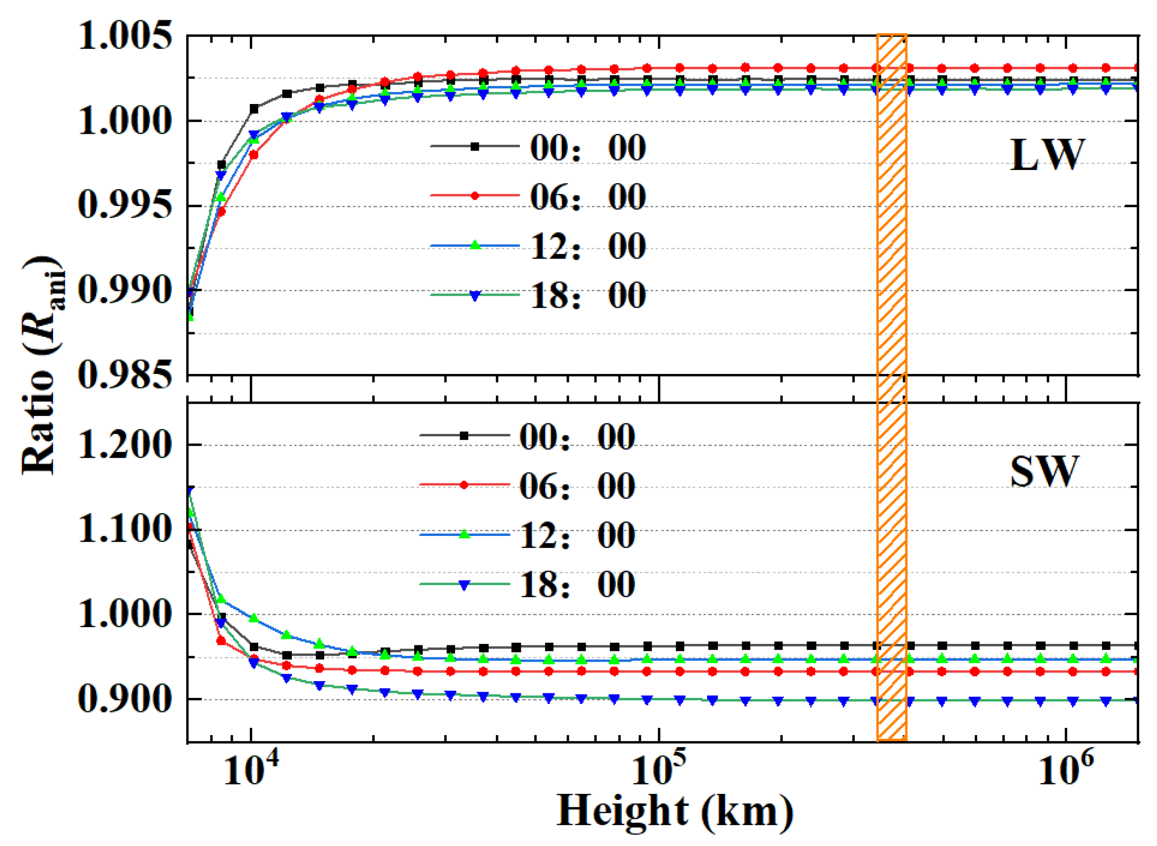
Figure 7 shows the ratio Rani (see Equation (7)) of the radiometer’s SW and LW EPIs at different heights at four moments on 1 January 2020. Due to the Rani being the ratio between the instantaneous anisotropic radiometer’s EPI and isotropic radiometer’s EPI, the size of Rani can be used to reflect the variation in the radiometer’s EPIs introduced by the ERBE ADMs and the platform’s heights. The GMAFs are determined by using the anisotropies characterized in the ERBE ADMs (as shown in Equations (8) – (15)), so the Rani can act as an indirect indicator of the GMAFs. When the platform height changes from 600 km to 1.5 × 10⁶ km, the Rani will vary from 0.986 to 1.003 for the LW, while for the SW, the value of Rani changes from 1.12~1.15 to 0.9~0.95. When the distance exceeds 3 × 10⁵ km (< Moon-based height—the orange rectangle frame in Figure 7), the variation in height will have an extremely small influence on the ratio Rani. Compared with the height, the four moments in Figure 7 mean that the MWFVR-viewed region is different, so the scene type and atmospheric conditions in the MWFVR-viewed scope will be the main influence factor for the radiometer’s SW and LW EPIs. It is worth noting that the ratio Rani for the outgoing LW and SW radiation is the value obtained on 1 January 2020 and the value will vary with time (see Figure 8).
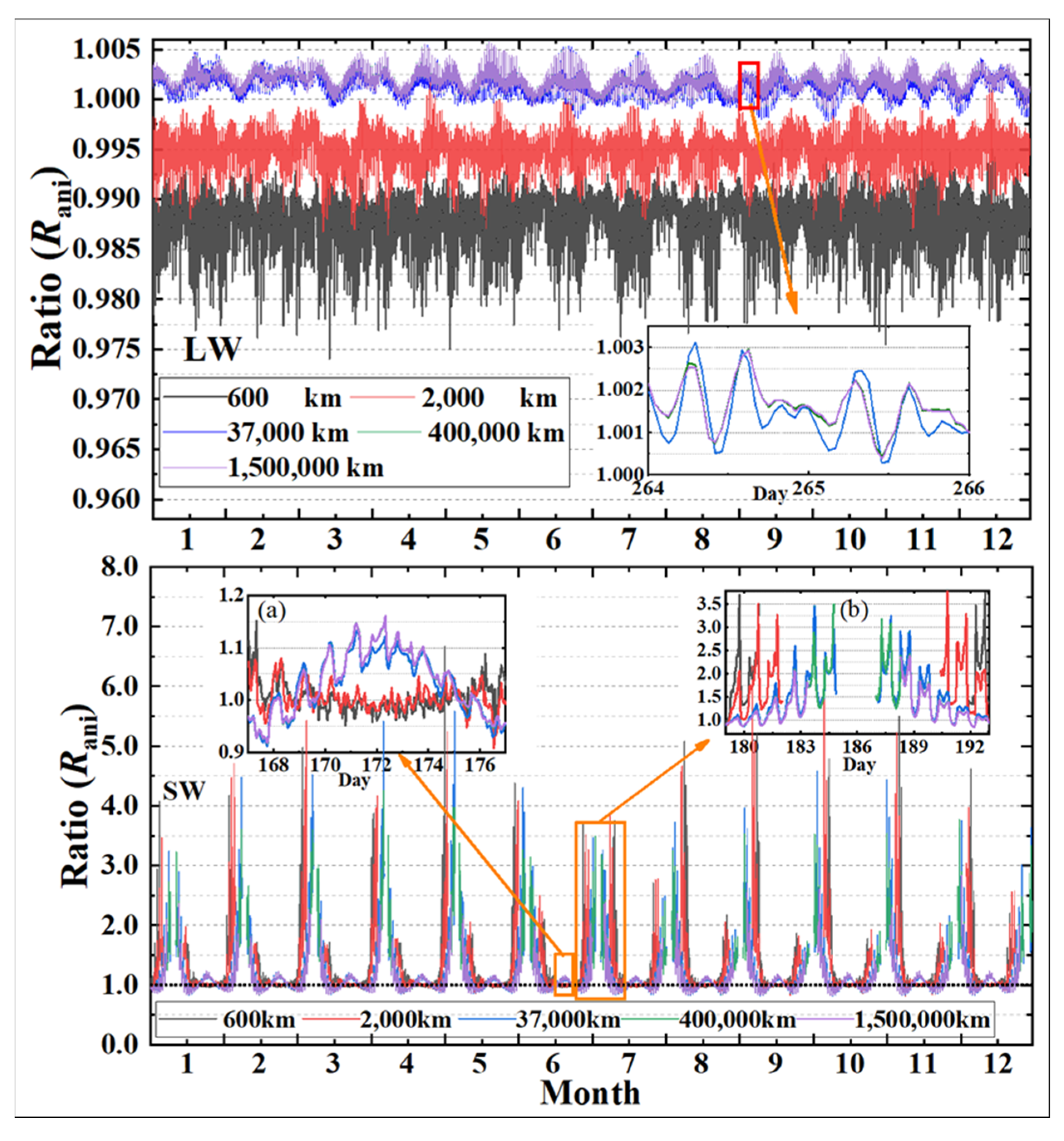
The time evolution of the Rani for the LW and SW at different heights in the year 2020 is plotted in Figure 8. For the LW, the lower the platform height, the larger the variation range of the Rani, and the more apparent period characteristics. With the increase in platform height, the radiometer-viewed region will enlarge and more outgoing radiant energy will arrive at the radiometer. The increased visible area in the radiometer’s scope also brings about an apparent diurnal and seasonal oscillation (Figure 8). In addition, when the platform’s height changes from 3.7 × 10⁴ km to 1.5 × 10⁶ km, the range of the LW Rani is 0.998~1.005. The height of the Moon-based platform varies from 3.5 × 10⁵ km to 4.1 × 10⁵ km, so the change in the LW Rani for MWFVR is less than 0.005. The SW ADMs are the function of the SZA, VZA, and RAA. Therefore, the various ranges of the SW Rani are larger than the value of LW. Similar to the Rani, the change range of the radiometer’s SW EPI is also larger than LW EPI. When the sunlit area in the MWFVR-viewed region is close to 0, the radiometer’s EPI is about 0 W·m−2 and the SW Rani changes more drastically, which can be observed by comparing the same moment in Figure 6 and Figure 8. For a detailed demonstration of the influence of height, the partially zoomed graphs are shown in Figure 8. The x-axis shows the days since 1 January 2020. For the LW, the zoomed graph reveals that the difference of the Rani is less than 0.001 when the height is greater than 3.7 × 10⁴ km. For the SW, the zoomed graph shows that the radiometer will have a longer observation duration for the sunlit portion in the direction of the Moon with the increase in platform height (see zoom (b) in Figure 8). When the radiometer-viewed region includes a 35% sunlit region, the range of Rani will remain between 0.9 and 1.2.
3.1.2. The Radiometer-Viewed Region
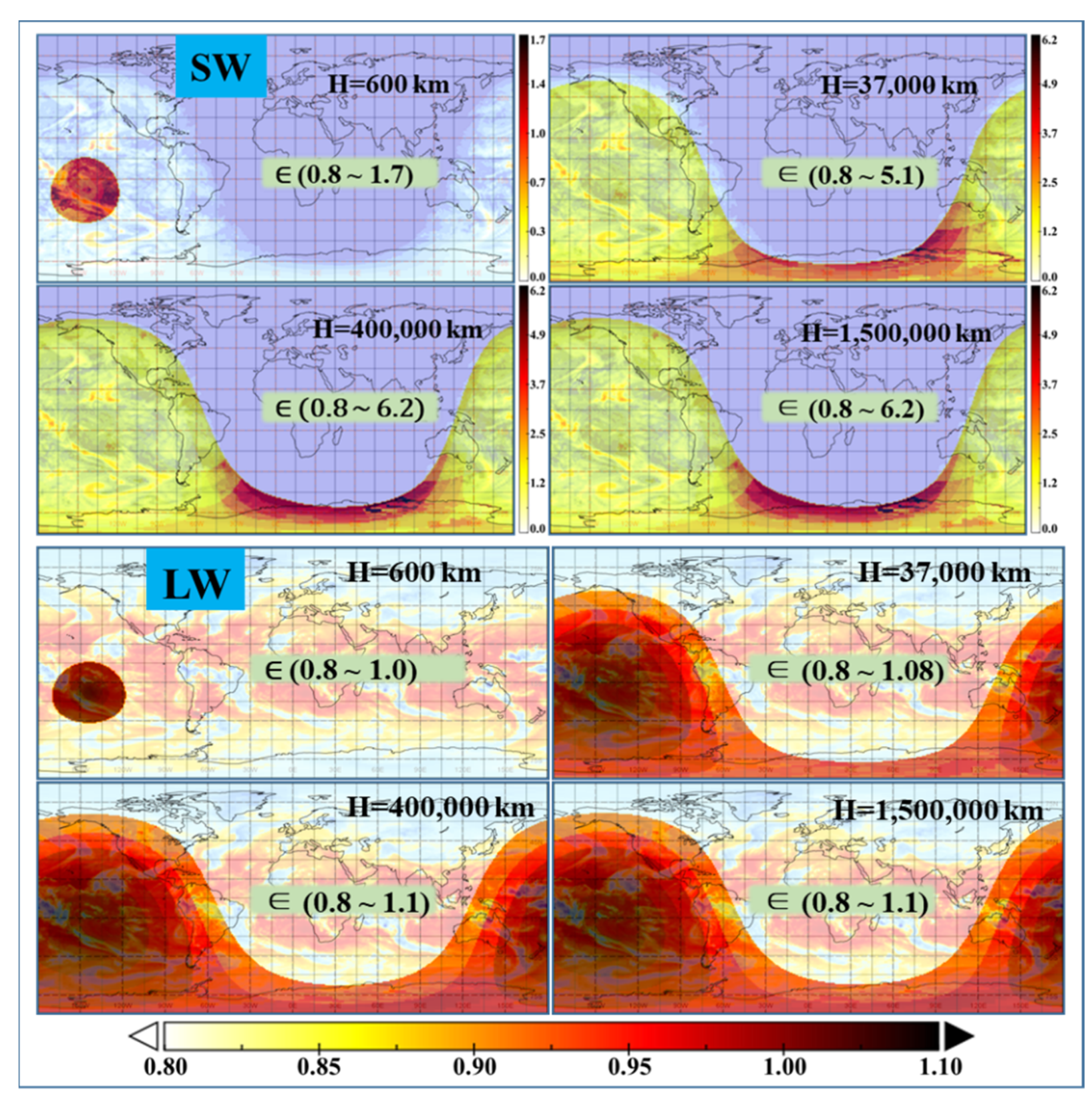
The distribution of outgoing LW radiation in the radiometer-viewed region at different heights shows that, for the LW, the field of view is centered on the sub-point and presents a circular distribution, and when the height is larger than 3.0 × 10⁵ km, the ratio of the radiometer-viewed region to the global is more than 49% and further increases in height do not significantly improve the visibility ratio. However, for the distribution of the SW radiation, it is more sensitive to the angle between the Sun vector and the Moon vector. Comparing the visible region of the MWFVR for the two heights of 4.0 × 10⁵ km and 1.5 × 10⁶ km, it can be found that when the distance increase by 3.75 times, the ratio of the radiometer-viewed sunlit region to the global sunlit area is improved no more than by 4%, and the enlarged field is entirely present in the margin, where it is mainly controlled by the Earth’s curvature. The difference in the platform’s height means that the LW and SW ADM distribution map will present a distinct feature, as shown in Figure 9. Figure 9 highlights the distribution of SW and LW anisotropic factors at four different heights on 23 January 2020, at 22:00. The background is the CERES radiative flux map at the same time. The brightness of the color represents the size of the value and the darker the color, the larger the value. The color scales between different subfigures are different and the responding ADM range is shown in the figures. Compared to the LW anisotropic factors (the value range: 0.8~1.1), the SW anisotropic factors have larger variations in spatial distribution and ranges (the value range: 0.8~6.2). For the SW, due to the anisotropic factors being the function of RAA, VZA, and SZA, the variation is more complex, as shown in Figure 9, and the maximum generally tends to occur at the fringes which are heavily affected by the Earth’s curvature. For the LW, the distribution of LW anisotropic factors exhibits a hemispherical characteristic. Although the position of the sub-radiometer point fluctuates with latitude on both sides of the equator, the sub-point always corresponds to the area where the anisotropic factor is the largest, and the farther away from the sub-satellite point, the smaller the value of the anisotropic factor. In summary, when the height of the radiometer is higher than a certain value, such as 3.0 × 10⁵ km, the change in both the visible region and the ADMs caused by the increase in the height has a weak influence on the irradiance, which means the irradiance can be compensated by simplified correction factors of K.
3.1.3. The SW Invisible Night Portion (Ad)
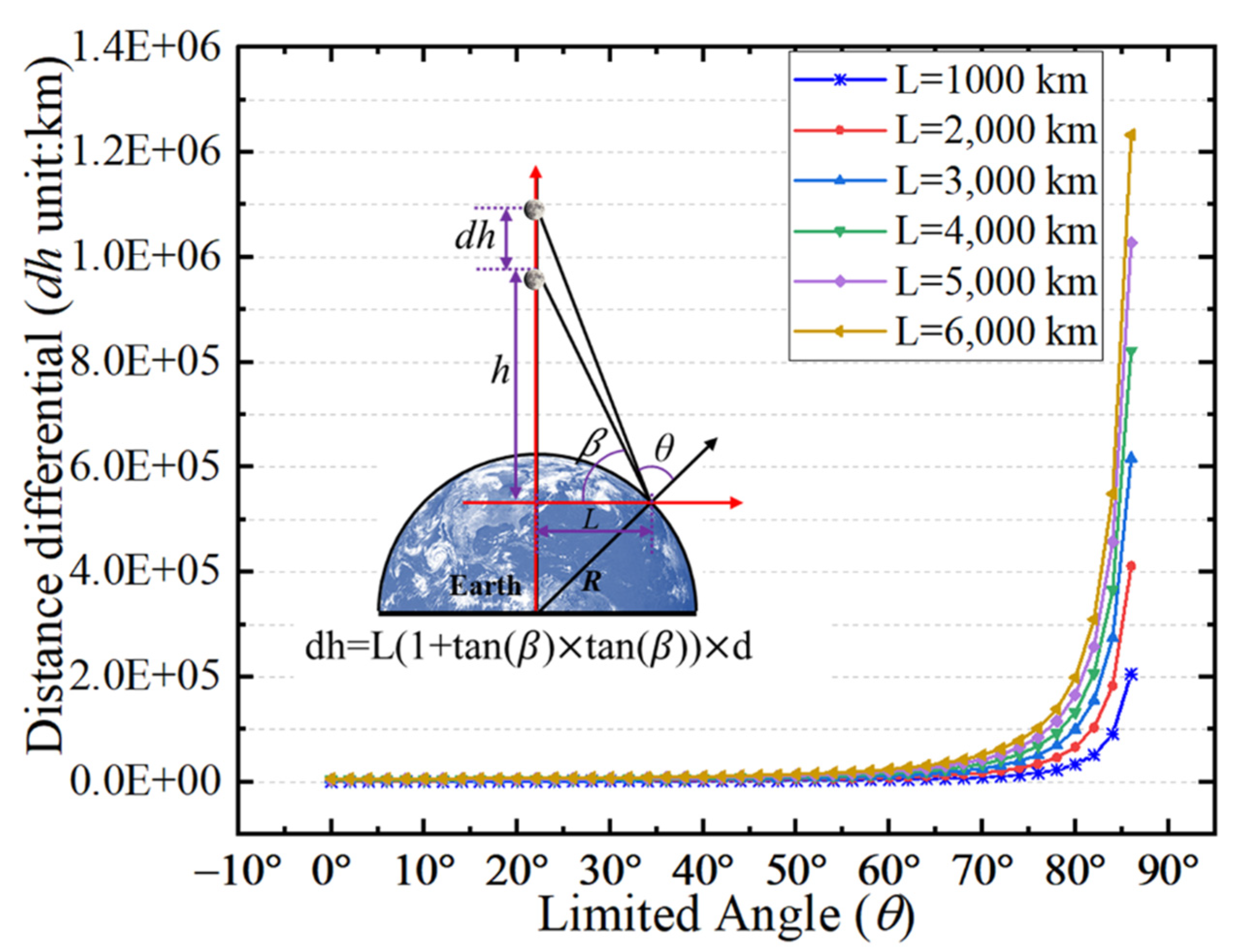
As seen from the analysis in Section 3.1.1 and Section 3.1.2, the increase in the satellite’s height will weaken the influence of ADMs and the radiometer-viewed region on the radiometer’s EPI. For the given scene and the radius of the field of view (supposed to be L ∈ (1,000 km, 6,000 km) as shown in Figure 10), the height h is the tangent function of the VZA (see Figure 2). From the derivative of the tangent function, it can be seen that when the angle θ is 80°, the change in the unit angle will lead to a change of 0.66 × 10⁵ km in height (dh), which is the equivalent quantity to the change value of the Earth–Moon distance (3.5 × 10⁵~4.1 × 10⁵ km). Because the Earth is close to a sphere with an average radius of approximately 6374 km, the curvature of the Earth will become a non-negligible factor and it also makes the contribution of the edge area to the radiometer much weaker than that of the central position.
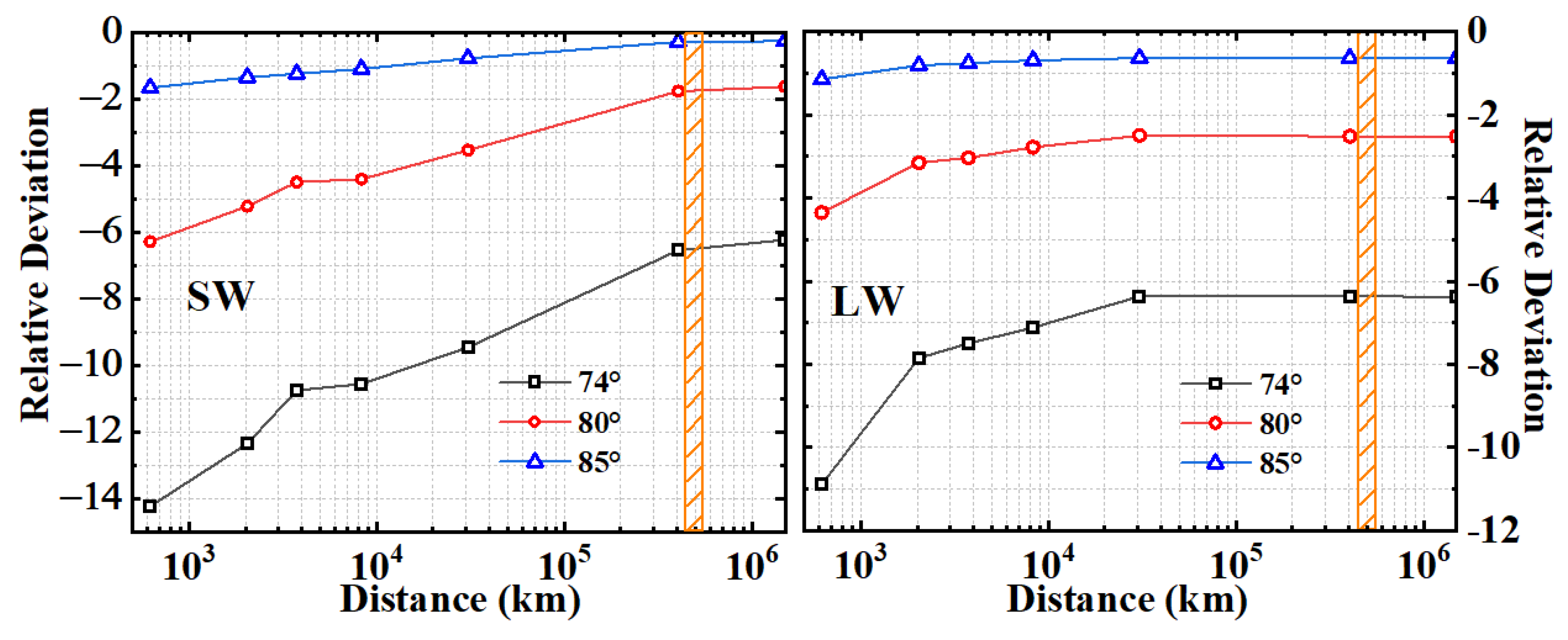
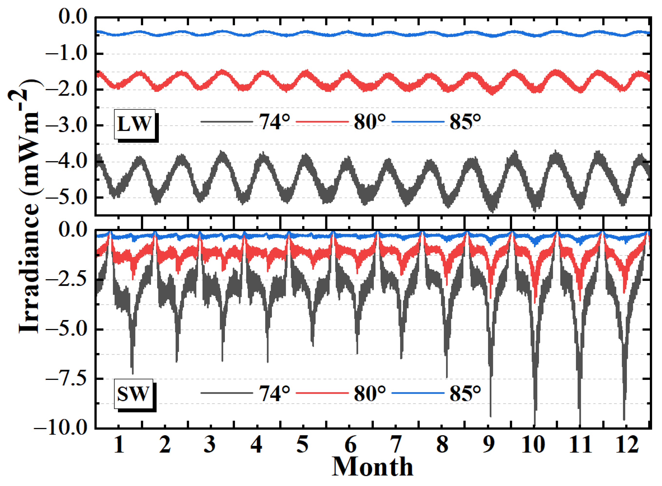
Figure 11 shows the relative deviation of the radiometer’s EPI at different heights on 23 January 2020, at 22:00, for three different limited angles θ of 74°, 80°, and 85° (see Figure 10). The relative deviation is calculated by comparing the above results with the result from the limited angle of 90°. In fact, the field-of-view of the MWFVR can capture the whole full disk of the Earth. Here, the purpose of the analysis of the limited angle only is to reveal the effects of expanding and shrinking the Earth’s margin regions on the radiometer’s EPI. The angle configuration of θ = 74° is based on the ERBE angle bin classifications, which guaranteed that the angle covers two different angle bins (see Table 1). The results indicate that for the given height, when the limited angle, θ, increases from 74° to 85°, the LW and SW EPIs’ relative deviation has an apparent decrease. For each limited angle, θ, the relative deviation will decline with the improvement in height. When the height is larger than 3 × 10⁵ km, the relative deviation remains essentially unchanged for the SW, and there exists a slight decline for the LW. When the limited angle θ is 85 degrees, the relative deviations of SW and LW are both less than 1.7%. For a longer period, such as one month, one year, or twenty years, the statistical results reveal that, for the Moon-based platform, the change ranges of LW EPI relative deviation are −6.5~−7.5% (74°), −3~−2% (80°), and −0.5~−0% (85°), respectively. However, for the SW, due to the sunlit portion being a variable with time, the change range of relative deviation is larger than LW and the values are −30~−5% (74°), −28~−0.5% (80°), and −16~−0.5%, respectively. Figure 12 presents the deviation of the radiometer’s EPI for different limited angles in 2020. The results show that, for the LW, the deviation ranges are −5.5~−3.55 mWm−2, −2.1~−1 mWm−2, and −0.55~−0.45 mWm−2 under three limited angles conditions, while for the SW, the deviation ranges are −10.0~−0.5 mWm−2, −3.75~−0.25 mWm−2, and −0.5~−0.0 mWm−2, respectively. Therefore, for the height of the MWFVR, when the limited angle changes from 85° to 90°, the irradiance deviation is less than 0.5 mWm−2.
3.2. The Analysis of Earth’s Outgoing Radiative Flux
3.2.1. The SW and LW GMAFs
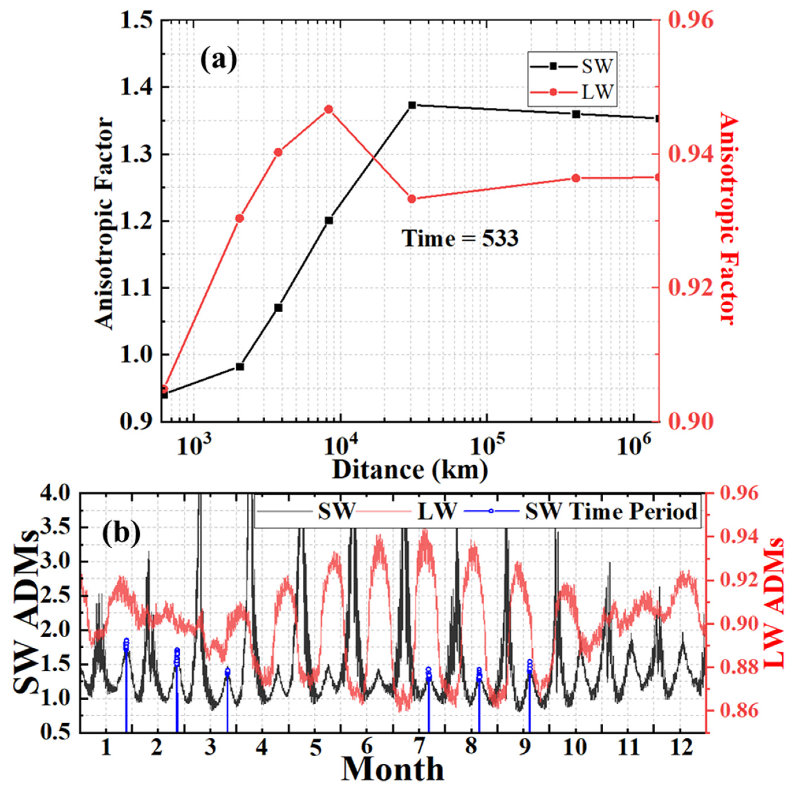
Based on the model established in this work, Figure 13 shows the SW and LW GMAFs (a) at different heights on 23 January 2017 and (b) on the Moon-based platform in 2017. Here, the choice of the data from 2017 is due to the NISTAR data, which will be used to compare the results between them. The results in Figure 13 show that the SW and LW GMAFs increase with the improvement in the platform’s height, and when the height is larger than 3 × 10⁵ km, the global mean SW and LW anisotropic factor is at a relatively stable level, which provides a possibility for the utilization of the model. For the LW, the GMAFs only change with the variation in geometry and radiometer-viewed region, and the range is 0.8593~0.9464, as shown in Figure 13b. However, because the sunlit portion in the radiometer-viewed region is a temporal variable, the method for calculation of the daytime Earth outgoing radiation is not suitable except for the specific periods, in which the angle of Moon–Earth–Sun is less than 5 degrees (see the blue line in Figure 13b). By detailed analysis, we acquired that the 5 degrees can ensure that the sunlit portion can account for 96.6% of the radiometer-viewed region. For the rest of the sunlit portion of the Earth’s TOA, only about 3.4% is not visible. According to the analysis in Section 3.1, the area correction factor method is adopted. Therefore, for the SW, the range of the GMAFs for the calculation periods is 1.267~1.805.
3.2.2. The Outgoing Radiative Flux without the Correction Factor K
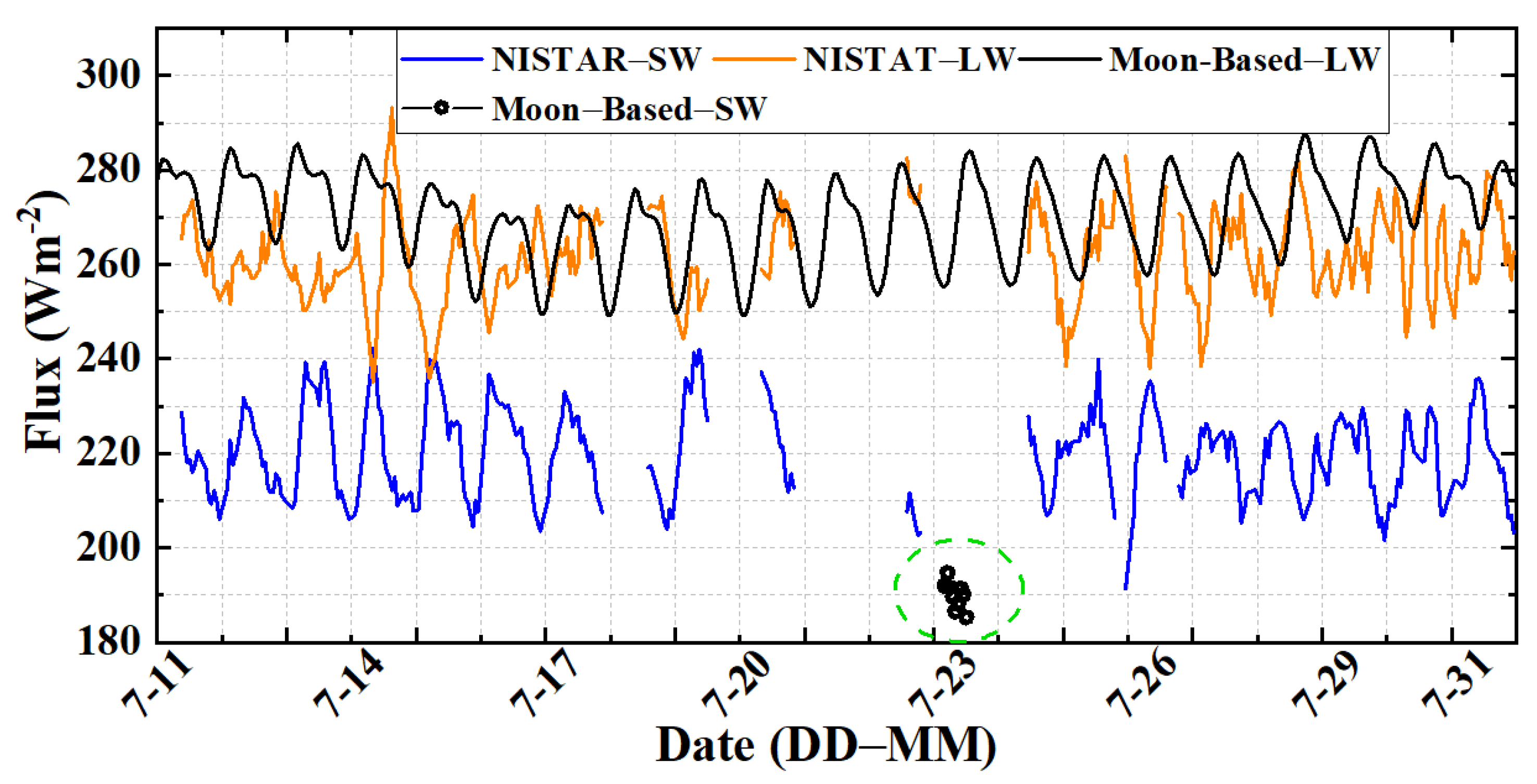
Here, only a part-time period (the angle of Sun–Earth–Moon ≤ 5 degrees) is used for ensuring the Earth’s outgoing radiative flux and validating the model. The remaining period needs to combine with the satellite-based data confirming the outgoing Earth radiative flux, which will be the focus of our future research. According to the results from Equation (12), the Moon-based radiometer data can efficiently capture the variation in distinct time scales for the outgoing radiative fluxes. The NISTAR measures Earth’s outgoing radiative fluxes with an accuracy of ~1.5% at the Lagrange-1 (L1) point (~1.5 million km). Therefore, the NISTAR data (https://asdc.larc.nasa.gov/data/DSCOVR/NIST/L2/FLX_01/, accessed on 26 November 2022) provide a suitable and reliable constraint and validation for the simulated Moon-based data. Figure 14 shows the outgoing radiative flux comparison between NISTAR data and the simulated Moon-based data not considering the correction factor K (see Equation (13)) for coincident observations of July 2017. The NISTAR LW fluxes vary around 235 and 293 Wm−2 for July, whereas the Moon-based counterparts are about 249 to 287 Wm−2. The maximum and minimum for the simulated Moon-based LW fluxes align with those LW fluxes from NISTAR data for analyses’ period moments. The simulated SW flux derived from Moon-based data presents a low level and the NISTAR SW fluxes oscillate around 191 and 242 Wm−2. However, the Moon-based SW counterparts are about 185 to 194 Wm−2 and the value is about 5 to 38 Wm−2 smaller compared with the NISTAR data, while the result is closer to the CERES data (188~215 Wm−2). Here, the reason for the smaller value for the simulated Moon-based data is that a small number of illuminated grid areas are not counted, so an area correction factor is introduced later to solve this problem.
3.2.3. The Earth’s Outgoing Radiative Flux
Because the orbit of the Moon is close to an ellipse (eccentricity ≈ 0.0549), the distance between the Moon and the Earth is a variable. The range of the Moon–Earth distance is about 3.5 × 10⁵~4.1 × 10⁵ km and the average value is 383,275 km, which results in a difference in the size of the Earth at different orbital positions, and the viewing zenith angle will vary with the time for the given region, as shown in Figure 2B and Figure 4. By analyzing the relationship between the limited angle deviation, θmax − θmin, for one position (see Figure 10) and the calculated position radius, the results reveal that the large observation distance change (the distance is around 6 × 10⁴ km from the perigee to the apogee) between the Moon and the Earth only causes the limited angle deviation, θmax − θmin, to vary from 0.002° to 0.121°, which means that the distance change does not change the distribution of ADMs for one moment, and the GMAFs only change with time and the viewed scene types. Here, the θmax and θmin are the angles when the dh in Figure 10 is equal to the maximum and minimum of the Earth–Moon distance. Therefore, for the convenience of processing and using the Moon-based data, we choose to transform the Moon-based data to a uniform height by multiplying distance and area correction factors. In other words, the release of the MWFVR’s data will be based on the average height (383,275 km) in the future, which will facilitate the comparison and collaborative utilization with low fixed-orbit satellite data.
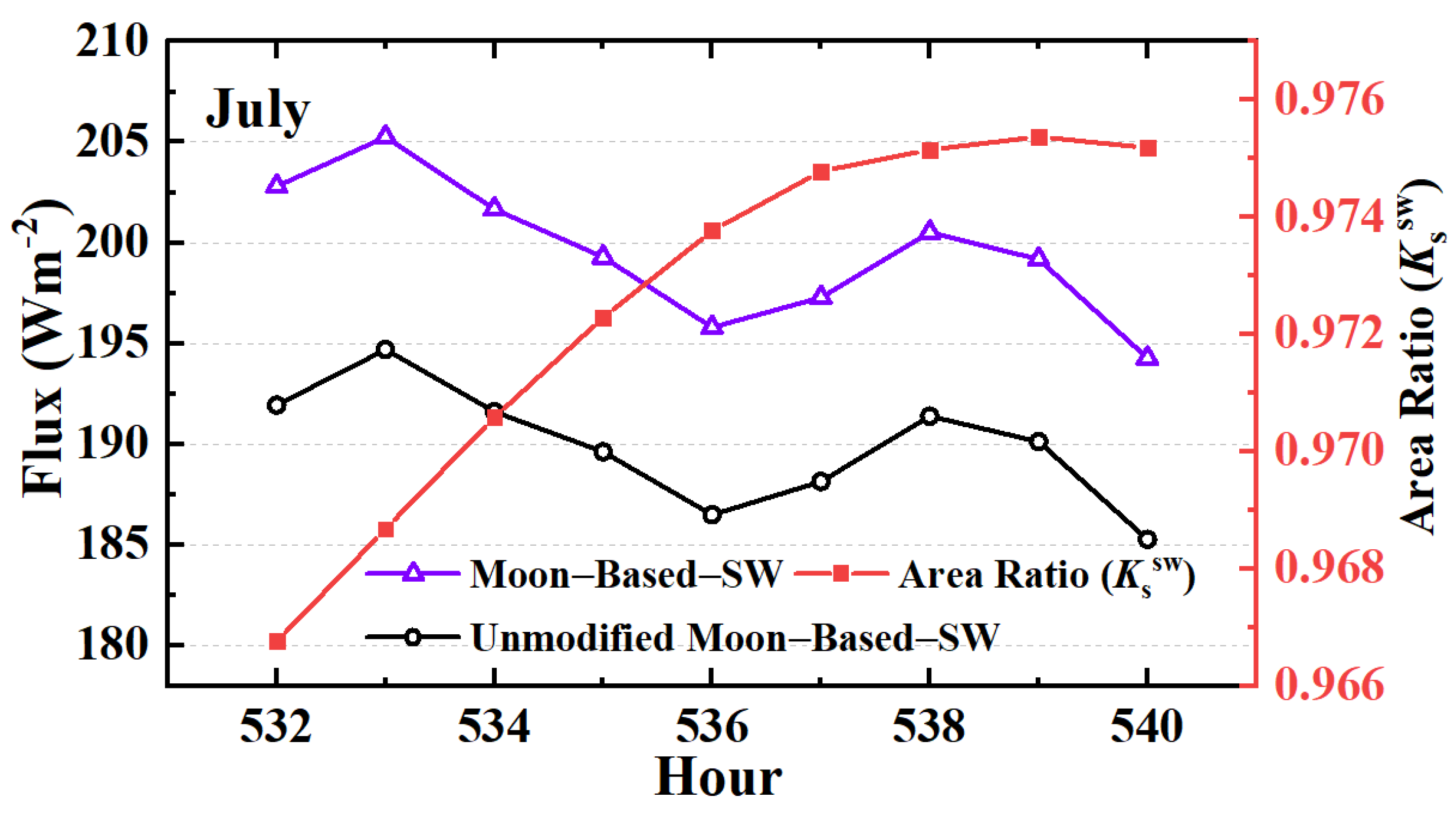
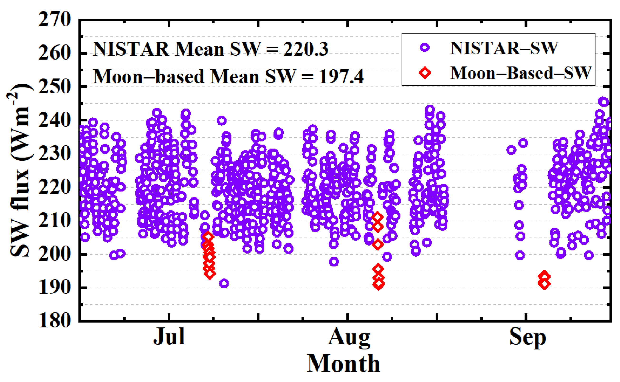
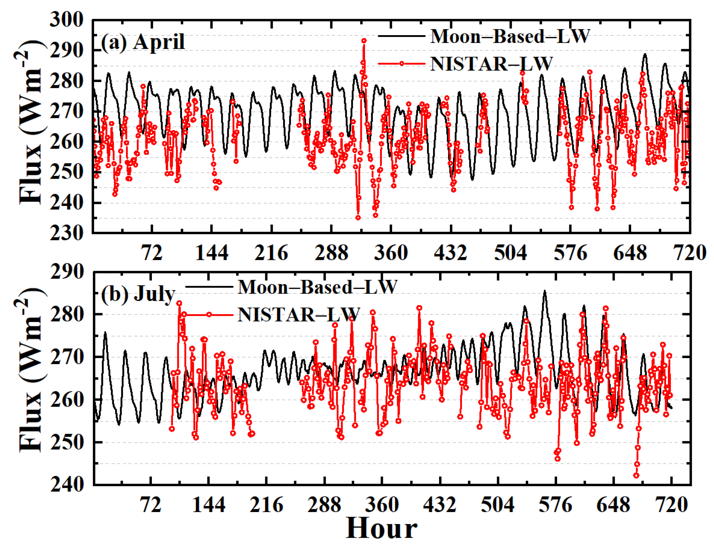
Figure 15 shows the comparison of the simulated Moon-based SW daytime outgoing radiative flux before and after correction. The modified results have an around 9.5 Wm−2 improvement. The SW flux range varies from 185~194 Wm−2 to 194~205 Wm−2, and the value is closer to the CERES data (188~215 Wm−2). Figure 16 compares the SW daytime outgoing radiative fluxes from NISTAR with those from the Moon-based data according to Equation (13) for July~September 2017. The NISTAR SW fluxes change from 191 to 242 Wm−2 with an average of 220.28 Wm−2, whereas the simulated Moon-based counterparts are about 5 to 20 Wm−2 smaller. The simulated SW fluxes from the MWFVR oscillate around 190 and 211 Wm−2 with an average of 197.4 Wm−2 and the result shows a much better agreement with those SW fluxes from CERES data compared to the NISTAR data. Due to the Moon-based data only existing in the specific periods, the Moon-based SW Earth’s outgoing radiative flux cannot capture the diurnal variation feature, but the data can act as the validation of low-orbit satellite data and ADMs. Moreover, to expand its usable time range and improve the calculation accuracy of the Earth’s outgoing radiative fluxes, we will try to use statistical results and empirical values to further improve the established model in this work. The LW flux comparisons between NISTAR data and simulated Moon-based data are shown in Figure 17. The NISTAR LW fluxes range from 239 to 289 Wm−2 for April and July, whereas the simulated Moon-based counterparts are 251~287 Wm−2. The simulated Moon-based LW fluxes’ differences between the daily maximum and minimum are typically more than 27 Wm−2; however, those daily LW fluxes’ differences from NISTAR data can vary from 10 to 50 Wm−2. This larger variability of NISTAR LW fluxes is because of noise and offset variabilities from both the total and SW channels. The simulated Moon-based LW radiative fluxes are consistently greater than CERES LW fluxes and they also show larger diurnal variations. The LW fluxes from the simulated Moon-based data and NISTAR data at all coincident hours of 2017 show that the mean LW fluxes are 260.8 and 265.3 Wm−2 for the NISTAR data and the simulated Moon-based data, respectively, and the root mean square (RMS) error is 12.6 Wm−2.
Table 2 and Table 3 summarize the monthly flux from the simulated Moon-based data, NISTAR data, and CERES SYN1deg data for July~September of 2017. The CERES SYN1deg data are calculated by using the method of latitude average. The simulated Moon-based SW fluxes are consistently greater than those SW fluxes from CERES SYN1deg data by about 0.5% to 1.6%, while the NISTAR SW fluxes are consistently greater than those from CERES SYN1deg data by about 7.8% to 13.5%. However, the simulated Moon-based SW fluxes are consistently smaller than those from NISTAR data by 10.1% to 11.5%. Furthermore, the correlation coefficients of SW fluxes between the CERES SYN1deg data and NISTAR data are about 0.89 and the correlation coefficients for the simulated Moon-based data and NISTAR data are 0.91, 0.63, and 0.53 for July~September, respectively. Due to the calculated time for Moon-based data being different from NISTAR, the correlation coefficient is calculated by the closest moment in nearby days. Moreover, July is well matched, and August and September are two days apart, but September also includes several hour match errors, which is the main reason for a smaller correlation coefficient. In addition, the simulated Moon-based data are closer to the CERES SYN1deg data from the RMS. For the LW flux, the simulated monthly Moon-based Earth’s outgoing radiative flux is closer to the NISTAR data, and the RMS between them is 2.61. Compared to the CERES SYN1deg data, the simulated monthly Moon-based data are about 10 to 20 Wm−2 greater. Moreover, the correlation for the LW fluxes is rather stable for the same period compared with SW fluxes and the correlation coefficients are 0.87, 0.69, and 0.61 for July to September 2017 (the calculation method is the same as SW fluxes).
3.3. Discussion
In this work, a model for estimating the Earth’s outgoing radiative flux from the MWFVR measurements is developed, and the unfiltered EPIs for the MWFVR are converted to full-disk LW and daytime SW outgoing radiative flux by accounting for the anisotropic characteristics of radiances. In the process of building the model framework, the influence of the height of the platform, the spatial-temporal distribution, and the limited angle on the Global Mean Anisotropic Factors (GMAFs) are analyzed and, finally, the feasibility and correctness of the estimating model are validated by comparing the results with the satellite-based data from the NISTAR and CERES SYN1deg datasets.
In the model, the confirmation of the GMAFs and the utilization of the correction factor are the key steps, so it is necessary to analyze the change features of the platform height and radiometer-viewed region. By studying the influence of platform height on irradiance time series, it can be found that as the height increases, the instrument-viewed region will increase and the effect of scene cover type will be weakened by mixing and overlaying. When the height exceeds 3 × 10⁵ km (<the Moon-based platform height), the variation in height will have a relatively small influence on the SW and LW ADMs, and the visible scene type will be the main influence factor. Moreover, the ratio of the area of the radiometer-viewed region to the global area is more than 49% and the further increases in height do not significantly improve the visibility ratio. Comparing the visible region for the two heights of 3.0 × 10⁵ km and 1.5 × 10⁶ km, it shows that the ratio of the radiometer-viewed sunlit region to the global sunlit area is improved by no more than 4% and the enlarged field is entirely present in the margin. For the height of the MWFVR, when the limited angle changes from 85° to 90°, the irradiance deviation is less than 0.5 mWm−2. When the height platform is larger than 3 × 10⁵ km, the global mean SW and LW anisotropic factor is at a relatively stable level. Moreover, the SW and LW GMAFs’ ranges for the calculation periods are 1.267~1.805 and 0.8593~0.9464, respectively. The distance change (around 6 × 10⁴ km) between the Moon and the Earth only causes the viewing zenith angle deviation, θmax − θmin, to vary from 0.002° to 0.121°, which means that the distance change does not change the distribution of ADMs for one moment, and the GMAFs only change with time and the viewed scene type. The purpose of the analysis of the influence of the height of the platform, the spatial-temporal distribution, and the limited angle on GMAFs is to reveal the reliability of the conduction of simplified correction factors, K. Therefore, for the MWFVR, the change in the height of the orbit will have a weak influence both on the visible field of view and the ADMs. For the convenience of processing the Moon-based data, we chose to transform the Moon-based data to a uniform height by multiplying distance and area correction factors.
To verify the correctness and usability of the model established in this work, the NISTAR and CERES SYN1deg data are used. The results reveal that the SW fluxes obtained from the Moon-based measurements are smaller than those from the NISTAR data, and the simulated Moon-based SW fluxes are about 5 to 20 Wm−2 smaller. The simulated Moon-based SW fluxes change from 190 to 211 Wm−2 with an average of 197.4 Wm−2 and the result shows a much better agreement with the CERES SYN1deg data than the NISTAR. The Moon-based and NISTAR LW fluxes are consistently greater than CERES LW fluxes. The correlation analysis shows that the coefficients of SW fluxes for Moon-based data and NISTAR data are 0.91, 0.63, and 0.53 for July, August, and September, respectively. Moreover, compared with the SW flux, the correlation of LW fluxes is more stable for the same period and the correlation coefficients are 0.87, 0.69, and 0.61 for July to September 2017. In summary, the Moon-based data can obtain valuable data on the Earth’s outgoing radiative fluxes, which provides an important data source for studying the Earth Radiation Budget.
In the work, we established a data processing model for the unfiltered EPI of a Moon-based radiometer to obtain the Earth’s outgoing radiative flux. To separate Short-Wave (SW) and Long-Wave (LW) data, the MWFVR will have four channels, including a total (LW + SW), a short-wave, and two calibrated channels. The SW channel is obtained by adding a quartz filter in front of the detector and the degradation of quartz filters can be checked by the calibrated channel. In addition, an Imaging Spectroradiometer must work with the radiometer simultaneously to provide accurate scene type, cloud, and aerosol information. The data of the Imaging Spectroradiometer will be used to invert the cloud characteristic parameters in different observation instrument-viewed regions, to facilitate the selection of ADMs and the processing of the Moon-based data. The instrument’s setup is similar to that of the EPIC on board the DSCOVR satellite. However, a limitation still exists in the model. The Moon-based measurements obtained from the wide field-view radiometer are filtered irradiances, so the influence of the filter transmission must be addressed in the future to derive any meaningful fluxes and the unfiltered algorithm needs to be developed for SW flux in the following work. The ERBE ADMs used in this work were derived from the Nimbus 7 Scanner and this set of ADMs is still being used in CERES data products. Although there exist some deficiencies in the detailed description of the changing characteristics of the ADMs, it is relatively mature for converting the radiance to a flux estimate when studying the ERB on a macro-scale, like the Moon-based platform, and still reflects the main features of the research issues. However, for the accurate calculation of Earth’s outgoing radiation, more detailed and precise scene-type-dependent ADMs are needed to characterize the global SW and LW anisotropy. Due to the cloud properties, like the cloud mask, cloud size, cloud area fraction, etc., and the aerosol having a strong influence on the outgoing radiation, the Imaging Spectroradiometer needs to work with the radiometer simultaneously for providing accurate scene type, cloud, and aerosol information, which is a crucial need for the choice of ADM. In addition, to validate the feasibility and correctness of the established estimating model, only a part-time period of the angle of the Sun–Earth–Moon being less than 5 degrees is used for the calculation of SW Earth’s outgoing radiative fluxes, which limits the radiometer to capture the long-term diurnal variation feature of Earth’s radiative fluxes. Therefore, to take full advantage of the remaining valuable Moon-based data, we will further improve the established model to expand its usable time range and the calculation accuracy of the Earth’s outgoing radiative fluxes in future work.
4. Conclusions
The Moon-based radiometer can provide continuous measurements for the Earth’s full-disk broadband irradiance. To measure the broadband Outgoing Short-Wave (SW) Radiation (OSR) and Long-Wave (LW) Radiation (OLR) from the Earth’s Top of the Atmosphere (TOA), the Earth usually is considered a single-pixel radiative source. In this work, a model for estimating the Earth’s outgoing radiative flux from Moon-based Wide Field-of-View Radiometer (MWFVR) measurements is developed, and the unfiltered entrance pupil irradiances for the MWFVR are converted to full-disk LW and daytime SW outgoing radiative flux by accounting for the anisotropic characteristics of radiances. In the process of building the model framework, the influence of the platform’s height, the spatial-temporal distribution, and the limited angle on the Global Mean Anisotropic Factors (GMAFs) are analyzed. Finally, the feasibility and correctness of the estimating model are validated by comparing the results with the satellite-based data from the NISTAR and CERES SYN1deg datasets.
In the model, the confirmation of the GMAFs and the utilization of the correction factor are the key steps. The results show that as the height increases, the instrument-viewed region will increase and the effect of scene cover type will be weakened by mixing and overlaying. When the height platform is larger than 3 × 10⁵ km, the global mean SW and LW anisotropic factor keeps a relatively stable level. Moreover, the SW and LW GMAFs’ ranges for the calculation periods are 1.267~1.805 and 0.8593~0.9464, respectively. The Earth–Moon distance change (around 6 × 10⁴ km) only causes the viewing zenith angle deviation, θmax − θmin, to vary from 0.002° to 0.121° (see Figure 10), which means that the distance change does not change the distribution of the angular distribution models (ADMs) for one moment, and the GMAFs only change with time and the viewed scene type. Therefore, for the MWFVR, the change in the height of the orbit will have a weak influence both on the visible field of view and the ADMs.
For the convenience of processing the Moon-based data, we chose to transform the Moon-based data to a uniform height by multiplying distance and area correction factors. The results show that the SW fluxes obtained from the Moon-based measurements are smaller than those from the NISTAR data, and the counterparts are about 5 to 20 Wm−2 smaller. The simulated Moon-based SW fluxes change from 190 to 211 Wm−2 with an average of 197.4 Wm−2 and the result shows a much better agreement with SW fluxes from the CERES SYN1deg data than the NISTAR data. The simulated Moon-based LW fluxes oscillate around 251 and 287 Wm−2 for April and July. Moreover, the Moon-based and NISTAR fluxes are consistently greater than CERES LW fluxes. The correlation analysis shows that the correlation coefficients of SW fluxes for Moon-based data and NISTAR data are 0.97, 0.63, and 0.53 for the months of July, August, and September, respectively. Compared with the SW flux, the correlation of LW fluxes is more stable for the same period and the correlation coefficients are 0.87, 0.69, and 0.61 for July to September 2017.
Author Contributions
Conceptualization, S.B. and S.D.; methodology, Y.Z.; software, Y.Z.; validation, Y.Z.; formal analysis, Y.Z.; investigation, Y.Z.; resources, Y.Z.; data curation, Y.Z.; writing—original draft preparation, Y.Z.; software, Y.Z.; writing—review and editing, S.B. and S.D.; supervision, S.B. and S.D.; project administration, S.B.; funding acquisition, S.B. All authors have read and agreed to the published version of the manuscript.
Funding
This research was funded by the Natural Science Basic Research Program of Shaanxi (No. 2023-JC-YB-389) and the National Natural Science Foundation of China (Grant No. 41590855, 51776171).
Institutional Review Board Statement
Not applicable.
Informed Consent Statement
All participants in the work were informed and consented to the publication of the paper.
Data Availability Statement
The Jet Propulsion Lab (JPL) Planetary and Lunar Ephemerides data used in this study were downloaded from the ephemeris system at https://ssd.jpl.nasa.gov/?planet_eph_export (accessed on 3 May 2020). The datasets of CER_SYN1deg-1Hour_Terra-Aqua-MODIS_Edition4A and CER_SYN1deg-1Hour_Terra-MODIS_Edition4A were downloaded from the online CERES data ordering system at https://asdc.larc.nasa.gov/project/CERES (accessed on 6 September 2021). The datasets of NISTAR Fluxes are download from https://asdc.larc.nasa.gov/data/DSCOVR/NIST/L2/FLX_01/, accessed on 26 November 2022).
Conflicts of Interest
The authors declare no conflict of interest.
References
- Stephens, G.L.; O’Brien, D.; Webster, P.J.; Pilewski, P.; Kato, S.; Li, J. The albedo of Earth. Rev. Geophys. 2015, 53, 141–163. [Google Scholar] [CrossRef] [Green Version]
- Ackerman, S.A.; Platnick, S.; Bhartia, P.K.; Duncan, B.; L’Ecuyer, T.; Heidinger, A.; Skofronick-Jackson, G.; Loeb, N.; Schmit, T.; Smith, N. Satellites See the World’s Atmosphere. Meteorol. Monogr. 2019, 59, 4.1–4.53. [Google Scholar] [CrossRef]
- Clerbaux, N.; Dewitte, S.; Bertrand, C.; Caprion, D.; De Paepe, B.; Gonzalez, L.; Ipe, A.; Russell, J.E.; Brindley, H. Unfiltering of the geostationary earth radiation budget (GERB) data. Part I: Shortwave radiation. J. Atmos. Ocean. Technol. 2008, 25, 1087–1105. [Google Scholar] [CrossRef]
- Clerbaux, N.; Dewitte, S.; Bertrand, C.; Caprion, D.; De Paepe, B.; Gonzalez, L.; Ipe, A.; Russell, J.E. Unfiltering of the geostationary earth radiation budget (GERB) data. Part II: Longwave radiation. J. Atmos. Ocean. Technol. 2008, 25, 1106–1117. [Google Scholar] [CrossRef] [Green Version]
- Dewitte, S.; Clerbaux, N. Measurement of the Earth radiation budget at the top of the atmosphere—A review. Remote Sens. 2017, 9, 1143. [Google Scholar] [CrossRef] [Green Version]
- House, F.B.; Gruber, A.; Hunt, G.E.; Mecherikunnel, A.T. History of satellite missions and measurements of the Earth radiation budget (1957–1984). Rev. Geophys. 1986, 24, 357–377. [Google Scholar] [CrossRef]
- Barkstrom, B.R.; Smith, G.L. The Earth Radiation Budget Experiment: Science and implementation. Rev. Geophys. 1984, 24, 379–390. [Google Scholar] [CrossRef]
- Doelling, D.R.; Sun, M.; Nordeen, M.L.; Haney, C.O.; Keyes, D.F.; Mlynczak, P.E. Advances in Geostationary-Derived Longwave Fluxes for the CERES Synoptic (SYN1deg) Product. J. Atmos. Ocean. Technol. 2016, 33, 503–521. [Google Scholar] [CrossRef]
- Doelling, D.R.; Loeb, N.G.; Keyes, D.F.; Nordeen, M.L.; Morstad, D.; Nguyen, C.; Wielicki, B.A.; Young, D.F.; Sun, M. Geostationary Enhanced Temporal Interpolation for CERES Flux Products. J. Atmos. Ocean. Technol. 2013, 30, 1072–1090. [Google Scholar] [CrossRef]
- Su, W.; Minnis, P.; Liang, L.; Duda, D.P.; Khlopenkov, K.; Thieman, M.M.; Yu, Y.; Smith, A.; Lorentz, S.; Feldman, D.; et al. Determining the daytime Earth radiative flux from National Institute of Standards and Technology Advanced Radiometer (NISTAR) measurements. Atmos. Meas. Tech. 2020, 13, 429–443. [Google Scholar] [CrossRef] [Green Version]
- Loeb, N.G.; Lyman, J.M.; Johnson, G.C.; Allan, R.P.; Doelling, D.R.; Wong, T.; Soden, B.J.; Stephens, G.L. Observed changes in top-of-the-atmosphere radiation and upper-ocean heating consistent within uncertainty. Nat. Geosci. 2012, 5, 110–113. [Google Scholar] [CrossRef]
- Stephens, G.L.; Li, J.-L.; Wild, M.; Clayson, C.A.; Loeb, N.G.; Kato, S.; L’Ecuyer, T.; Stackhouse, P.W.; Lebsock, M.; Andrews, T. An update on Earth’s energy balance in light of the latest global observations. Nat. Geosci. 2012, 5, 691–696. [Google Scholar] [CrossRef]
- Duan, W.; Huang, S.; Nie, C. Entrance pupil irradiance estimating model for a moon-based Earth radiation observatory instrument. Remote Sens. 2019, 11, 583. [Google Scholar] [CrossRef] [Green Version]
- Lohmeyer, W.Q.; Cahoy, K. Space weather radiation effects on geostationary satellite solid-state power amplifiers. Space Weather 2013, 11, 476–488. [Google Scholar] [CrossRef] [Green Version]
- Durante, M.; Cucinotta, F.A. Physical basis of radiation protection in space travel. Rev. Mod. Phys. 2011, 83, 1245. [Google Scholar] [CrossRef]
- Li, C.; Wang, C.; Wei, Y.; Lin, Y. China’s present and future lunar exploration program. Science 2019, 365, 238–239. [Google Scholar] [CrossRef] [PubMed]
- Guo, H.; Liu, G.; Ding, Y. Moon-based Earth observation: Scientific concept and potential applications. Int. J. Digit. Earth 2018, 11, 546–557. [Google Scholar] [CrossRef]
- Yan, Y.; Wang, H.N.; He, H.; He, F.; Chen, B.; Feng, J.Q.; Ping, J.S.; Shen, C.; Xu, R.L.; Zhang, X.X. Analysis of observational data from Extreme Ultra-Violet Camera onboard Chang’E-3 mission. Astrophys. Space Sci. 2016, 361, 76. [Google Scholar] [CrossRef]
- Zhang, Y.; Bi, S.; Wu, J. The influence of lunar surface position on irradiance of moon-based earth radiation observation. Front. Earth Sci. 2022, 16, 757–773. [Google Scholar] [CrossRef]
- Ye, H.; Guo, H.; Liu, G.; Ren, Y. Observation duration analysis for Earth surface features from a Moon-based platform. Adv. Space Res. 2018, 62, 274–287. [Google Scholar] [CrossRef]
- Zhang, Y.; Bi, S.; Wu, J. Effect of Temporal Sampling Interval on the Irradiance for Moon-Based Wide Field-of-View Radiometer. Sensors 2022, 22, 1581. [Google Scholar] [CrossRef] [PubMed]
- Huang, J.; Guo, H.; Liu, G.; Shen, G.; Ye, H.; Deng, Y.; Dong, R. Spatio-Temporal Characteristics for Moon-Based Earth Observations. Remote Sens. 2020, 12, 2848. [Google Scholar] [CrossRef]
- Huang, J.; Guo, H.; Liu, G.; Wang, H.; Deng, Y.; Dong, R. Observational angular analysis of Moon-based Earth observations. Int. J. Remote Sens. 2022, 43, 2315–2333. [Google Scholar] [CrossRef]
- Sui, Y.; Guo, H.; Liu, G.; Ren, Y. Analysis of Long-Term Moon-Based Observation Characteristics for Arctic and Antarctic. Remote Sens. 2019, 11, 2805. [Google Scholar] [CrossRef] [Green Version]
- Chen, G.; Guo, H.; Jiang, H.; Han, C.; Ding, Y.; Wu, K. Analysis of Comprehensive Multi-Factors on Station Selection for Moon-Based Earth Observation. Remote Sens. 2022, 14, 5404. [Google Scholar] [CrossRef]
- Yuan, L.; Liao, J. A physical-based algorithm for retrieving land surface temperature from Moon-based Earth observation. IEEE J. Sel. Top. Appl. Earth Obs. Remote Sens. 2020, 13, 1856–1866. [Google Scholar] [CrossRef]
- Swartz, B.H.; Dyrud, L.P.; Lorentz, S.R.; Wu, D.G.; Wiscombe, W.J.; Papadakis, S.J. The RAVAN CubeSat mission: Progress toward a new measurement of Earth outgoing radiation. In AGU Fall Meeting Abstracts, Proceedings of the AGU Fall Meeting, San Francisco, CA, USA, 15–19 December 2014; American Geographical Union: Washington, DC, USA, 2014; p. A22F-04. [Google Scholar]
- Schifano, L.; Smeesters, L.; Geernaert, T.; Berghmans, F.; Dewitte, S. Design and Analysis of a Next-Generation Wide Field-ofView Earth Radiation Budget Radiometer. Remote Sens. 2020, 12, 425. [Google Scholar] [CrossRef] [Green Version]
- Loeb, N.G.; Doelling, D.R.; Wang, H.; Su, W.; Nguyen, C.; Corbett, J.G.; Liang, L.; Mitrescu, C.; Rose, F.G.; Kato, S. Clouds and the earth’s radiant energy system (CERES) energy balanced and filled (EBAF) top-of-atmosphere (TOA) edition-4.0 data product. J. Clim. 2018, 31, 895–918. [Google Scholar] [CrossRef]
- Suttles, J.T.; Green, R.N.; Minnis, P.; Smith, G.; Staylor, W.; Wielicki, B.; Walker, I.J.; Young, D.F.; Taylor, V.R.; Stowe, L. Angular Radiation Models for Earth-Atmosphere System; Shortwave Radiation; National Aeronautics and Space Administration: Washington, DC, USA, 1988; Volume 1. [Google Scholar]
- Suttles, J.T.; Green, R.N.; Smith, G.L.; Wielicki, B.A.; Walker, I.J.; Taylor, V.R.; Stowe, L.L. Angular Radiation Models for Earth-Atmosphere System; Longwave Radiation; National Aeronautics and Space Administration: Washington, DC, USA, 1989; Volume 2. [Google Scholar]
- Su, W.; Corbett, J.; Eitzen, Z.; Liang, L. Next-generation angular distribution models for top-of-atmosphere radiative flux calculation from CERES instruments: Methodology. Atmos. Meas. Tech. 2015, 8, 611–632. [Google Scholar] [CrossRef] [Green Version]
- Su, W.; Corbett, J.; Eitzen, Z.; Liang, L. Next-generation angular distribution models for top-of-atmosphere radiative flux calculation from CERES instruments: Validation. Atmos. Meas. Tech. 2015, 8, 3297–3313. [Google Scholar] [CrossRef] [Green Version]
- Gristey, J.J.; Su, W.; Loeb, N.G.; Vonder Haar, T.H.; Tornow, F.; Schmidt, S.K.; Hakuba, M.Z.; Pilewskie, P.; Russell, J.E. Shortwave Radiance to Irradiance Conversion for Earth Radiation Budget Satellite Observations: A Review. Remote Sens. 2021, 13, 2640. [Google Scholar] [CrossRef]
- Park, R.S.; Folkner, W.M.; Williams, J.G.; Boggs, D.H. The JPL planetary and lunar ephemerides DE440 and DE441. Astron. J. 2021, 161, 105. [Google Scholar] [CrossRef]
- Petit, G.; Luzum, B. IERS- IERS Conventions (2010). International Earth Rotation and Reference Systems Service (IERS) Technical Note. 2016. Available online: https://www.iers.org/IERS/EN/Publications/TechnicalNotes/tn36.html (accessed on 27 January 2020).
- Wu, J.; Guo, H.; Ding, Y.; Shang, H.; Li, T.; Li, L.; Lv, M. The Influence of Anisotropic Surface Reflection on Earth’s Outgoing Shortwave Radiance in the Lunar Direction. Remote Sens. 2022, 14, 887. [Google Scholar] [CrossRef]
- Smith, G.L.; Priestley, K.J.; Loeb, N.G.; Wielicki, B.A.; Charlock, T.P.; Minnis, P.; Doelling, D.R.; Rutan, D.A. Clouds and Earth Radiant Energy System (CERES), a review: Past, present and future. Adv. Space Res. 2011, 48, 254–263. [Google Scholar] [CrossRef]
- Wielicki, B.A.; Barkstrom, B.R.; Harrison, E.F.; Lee, R.B., III; Smith, G.L.; Cooper, J.E. Clouds and the Earth’s Radiant Energy System (CERES): An Earth observing system experiment. Bull. Am. Meteorol. Soc. 1996, 77, 853–868. [Google Scholar] [CrossRef]
Figure 1.
The observation geometry of the MWFVR.

Figure 2.
(A) The sketch illustrates the irradiance and the angular coordinate system for angular distribution models. (B) The diagram for showing the viewing zenith angle differences among distinct platforms at different heights.
Figure 2.
(A) The sketch illustrates the irradiance and the angular coordinate system for angular distribution models. (B) The diagram for showing the viewing zenith angle differences among distinct platforms at different heights.

Figure 3.
The anisotropic factors from ERBE ADMs ((a,b): SW, (c,d): LW).

Figure 4.
(a) Schematic of the Earth–Sun–Moon geometry and Earth disk visible to the Moon-based view. (b) Diagram of the orbits for the LEO, GEO, and Moon.
Figure 4.
(a) Schematic of the Earth–Sun–Moon geometry and Earth disk visible to the Moon-based view. (b) Diagram of the orbits for the LEO, GEO, and Moon.

Figure 5.
The calculation framework of the Earth outgoing radiative flux estimating model. ADMs: angular distribution models.
Figure 5.
The calculation framework of the Earth outgoing radiative flux estimating model. ADMs: angular distribution models.

Figure 6.
The simulated radiometer’s EPI under two conditions, anisotropy and isotropy, at different heights in January 2020. (a–f) are the LW/SW EPI at the height of H, respectively. The zoomed graph in subfigure (d) is an extended demonstration of the difference between anisotropy and isotropy.
Figure 6.
The simulated radiometer’s EPI under two conditions, anisotropy and isotropy, at different heights in January 2020. (a–f) are the LW/SW EPI at the height of H, respectively. The zoomed graph in subfigure (d) is an extended demonstration of the difference between anisotropy and isotropy.

Figure 7.
The ratio Rani under two conditions, anisotropy and isotropy, for the LW and SW outgoing radiation at different heights in four moments on 1 January 2020. The orange rectangle frame is the height range of the MWFVR.
Figure 7.
The ratio Rani under two conditions, anisotropy and isotropy, for the LW and SW outgoing radiation at different heights in four moments on 1 January 2020. The orange rectangle frame is the height range of the MWFVR.

Figure 8.
The ratio Rani for the radiometer’s LW and SW EPI at different heights in the year 2020. The x-axis shows the days since 1 January 2020 for partially zoomed graphs. The partially zoomed graphs are shown for the presentation of detailed information.
Figure 8.
The ratio Rani for the radiometer’s LW and SW EPI at different heights in the year 2020. The x-axis shows the days since 1 January 2020 for partially zoomed graphs. The partially zoomed graphs are shown for the presentation of detailed information.

Figure 9.
The distribution of short-wave and long-wave anisotropic factors at different heights on 23 January 2020, at 22:00.
Figure 9.
The distribution of short-wave and long-wave anisotropic factors at different heights on 23 January 2020, at 22:00.

Figure 10.
The distance differential at different Earth surface locations for different limited angles.
Figure 10.
The distance differential at different Earth surface locations for different limited angles.

Figure 11.
The relative deviation of irradiance at different heights on 23 January 2020, at 22:00, for different limited angles. The orange bar is the variation range of the Earth-Moon distance.
Figure 11.
The relative deviation of irradiance at different heights on 23 January 2020, at 22:00, for different limited angles. The orange bar is the variation range of the Earth-Moon distance.

Figure 12.
The deviation of irradiance for different limited angles in 2020.

Figure 13.
The SW and LW GMAFs (a) at different heights on 23 January 2017 and (b) at the Moon-based platform in 2017.
Figure 13.
The SW and LW GMAFs (a) at different heights on 23 January 2017 and (b) at the Moon-based platform in 2017.

Figure 14.
The SW and LW daytime outgoing radiative flux comparison of NISAR data and the simulated Moon-based data in July 2017 did not consider the correction factor K. The green circle is the Moon-based shortwave flux data.
Figure 14.
The SW and LW daytime outgoing radiative flux comparison of NISAR data and the simulated Moon-based data in July 2017 did not consider the correction factor K. The green circle is the Moon-based shortwave flux data.

Figure 15.
The comparison of the Moon-based SW daytime outgoing radiative flux before and after correction and the red line presents the area ratio of .
Figure 15.
The comparison of the Moon-based SW daytime outgoing radiative flux before and after correction and the red line presents the area ratio of .

Figure 16.
The SW flux (Wm−2) from the NISTAR and Moon-based data for July, August, and September 2017.
Figure 16.
The SW flux (Wm−2) from the NISTAR and Moon-based data for July, August, and September 2017.

Figure 17.
The LW fluxes (Wm−2) from NISTAR data and simulated Moon-based data for April (a) and July (b) 2017.
Figure 17.
The LW fluxes (Wm−2) from NISTAR data and simulated Moon-based data for April (a) and July (b) 2017.

Table 1.
The illustration of ERBE ADM scene types and angular bin definitions of viewing zenith angle [31].
Table 1.
The illustration of ERBE ADM scene types and angular bin definitions of viewing zenith angle [31].
| Scene Bin | Scene | Cloud Fraction Range | Angle Bin | Viewing Zenith Angle Range |
|---|---|---|---|---|
| 1 | Clear Ocean | 0.00–0.05 | 1 | 0~15 |
| 2 | Clear Land | 0.00–0.05 | 2 | 15~27 |
| 3 | Clear Snow | 0.00–0.05 | 3 | 27~39 |
| 4 | Clear Desert | 0.00–0.05 | 4 | 39~51 |
| 5 | Clear Land–Ocean Mix (Coastal) | 0.00–0.05 | 5 | 51~63 |
| 6 | Partly Cloudy Over Ocean | 0.05–0.50 | 6 | 63~75 |
| 7 | Partly Cloudy Over Land or Desert | 0.05–0.50 | 7 | 75~90 |
| 8 | Partly Cloudy Over Land–Ocean Mix | 0.05–0.50 | ||
| 9 | Mostly Cloudy Over Ocean | 0.50–0.95 | ||
| 10 | Mostly Cloudy Over Land or Desert | 0.50–0.95 | ||
| 11 | Mostly Cloudy Over Land–Ocean Mix | 0.50–0.95 | ||
| 12 | Overcast | 0.95–1.00 |
Disclaimer/Publisher’s Note: The statements, opinions and data contained in all publications are solely those of the individual author(s) and contributor(s) and not of MDPI and/or the editor(s). MDPI and/or the editor(s) disclaim responsibility for any injury to people or property resulting from any ideas, methods, instructions or products referred to in the content. |
© 2023 by the authors. Licensee MDPI, Basel, Switzerland. This article is an open access article distributed under the terms and conditions of the Creative Commons Attribution (CC BY) license (https://creativecommons.org/licenses/by/4.0/).
Share and Cite
MDPI and ACS Style
Zhang, Y.; Dewitte, S.; Bi, S. A Model for Estimating the Earth’s Outgoing Radiative Flux from A Moon-Based Radiometer. Remote Sens. 2023, 15, 3773. https://doi.org/10.3390/rs15153773
AMA Style
Zhang Y, Dewitte S, Bi S. A Model for Estimating the Earth’s Outgoing Radiative Flux from A Moon-Based Radiometer. Remote Sensing. 2023; 15(15):3773. https://doi.org/10.3390/rs15153773
Chicago/Turabian StyleZhang, Yuan, Steven Dewitte, and Shengshan Bi. 2023. "A Model for Estimating the Earth’s Outgoing Radiative Flux from A Moon-Based Radiometer" Remote Sensing 15, no. 15: 3773. https://doi.org/10.3390/rs15153773
Note that from the first issue of 2016, this journal uses article numbers instead of page numbers. See further details here.