
Deep Image Prior Amplitude SAR Image Anonymization
by
 , , , and
Edoardo Daniele Cannas
1,*,
Sara Mandelli
1,
Paolo Bestagini
1,
Stefano Tubaro
1 and
Edward J. Delp
2 1
Dipartimento di Elettronica, Informazione e Bioingegneria (DEIB), Politecnico di Milano, 20133 Milan, Italy
2
School of Electrical and Computer Engineering, Purdue University, West Lafayette, IN 47907, USA
*
Author to whom correspondence should be addressed.
Remote Sens. 2023, 15(15), 3750; https://doi.org/10.3390/rs15153750
Submission received: 31 May 2023
/
Revised: 11 July 2023
/
Accepted: 21 July 2023
/
Published: 27 July 2023
(This article belongs to the Special Issue SAR Images Processing and Analysis)
Abstract
:This paper presents an extensive evaluation of the Deep Image Prior (DIP) technique for image inpainting on Synthetic Aperture Radar (SAR) images. SAR images are gaining popularity in various applications, but there may be a need to conceal certain regions of them. Image inpainting provides a solution for this. However, not all inpainting techniques are designed to work on SAR images. Some are intended for use on photographs, while others have to be specifically trained on top of a huge set of images. In this work, we evaluate the performance of the DIP technique that is capable of addressing these challenges: it can adapt to the image under analysis including SAR imagery; it does not require any training. Our results demonstrate that the DIP method achieves great performance in terms of objective and semantic metrics. This indicates that the DIP method is a promising approach for inpainting SAR images, and can provide high-quality results that meet the requirements of various applications.
1. Introduction
Synthetic Aperture Radar (SAR) images are a powerful tool for studying the Earth’s surface [1]. They are radar signals generated by an imaging system mounted on a platform such as an aircraft or satellite. As the platform moves, the system emits sequentially high-power electromagnetic waves through its antenna. The waves are then reflected by the Earth’s surface, re-captured by the antenna, and finally processed to create detailed images of the terrain below.
SAR images are employed in a wide variety of applications [2,3]. Indeed, as the waves hit different objects, their phase and amplitude are modified according to the objects’ characteristics (e.g., permittivity, roughness, geometry, etc.). The collected signal provides highly detailed information about the shape and elevation of the Earth’s surface. SAR images are also used for monitoring natural disasters, such as earthquakes, floods, and landslides, as well as for detecting changes in land-use patterns, such as urbanization and deforestation. Due to their nature of providing detailed imagery regardless of daylight and weather conditions, SAR images are also a precious asset in military applications [3]. As a matter of fact, SAR images can be used to detect sensible military targets like aircrafts [4], airports [5], ships [6], tanks or other vehicles [7].
In recent years, SAR images have become more widely available than ever before. Many portals now offer SAR images for free, making them accessible to researchers, students, and the general public alike [8,9,10]. This has led to a surge in research using SAR imagery and increased deployment of this technology in commercial products and services.
The research community is concerned about the potential misuse of SAR images, which play a critical role in many applications, particularly military ones. The widespread availability of SAR images means that almost anyone can extract sensitive information from them, such as the location of troops or civilians during a conflict [11]. As a result, some providers have begun to conceal features and information in their geospatial services, such as hiding traffic from maps that could reveal the location of refugees [12].
All these elements make it clear that techniques that anonymize or conceal target areas from remote sensing raster data are necessary. With this goal in mind, in this paper, we tackle the problem of removing sensitive objects from amplitude SAR images while preserving most of their content from a semantic point of view, i.e., most of their land-cover content.
We accomplish this task by relying on Deep Learning (DL) techniques for analyzing and processing SAR images. As a matter of fact, in recent years the SAR research community has gained a particular interest in DL tools like Convolutional Neural Networks (CNNs) due to their ability to learn complex features directly from data without manual processes involved. Recently, DL has been exploited for SAR image de-speckling [13], land-cover classification, oil spills detection [14,15], change detection of land use patterns [16,17,18], and so forth.
Also, the generation of SAR images using CNNs has found some compelling applications. Guo et al. [19] relied on Generative Adversarial Networks (GANs) for generating fully synthetic SAR images of military vehicles starting from simple observation parameters like platform azimuth and target depression angles. Baier et al. [20] generated both SAR and RGB satellite images by providing as inputs land-cover maps and digital elevation models to a conditional GAN. Moreover, there have been several other contributions exploiting RGB data to synthesize SAR images and vice versa [21,22,23], as well as methods exploiting SAR images to improve the quality of Electro-Optical (EO) images [24,25,26].
All these DL-based solutions typically need a training phase for the CNN to “learn” how to properly process the data for the task at hand. Training involves the collection of a corpus of data to optimize the parameters of the networks. This data collection must contain a considerable amount of samples to be representative of the data distribution in the real world, and to allow for the creation of training, validation, and test splits to avoid overfitting. Depending on the dimensions of the datasets, the complexity of the architecture, and the training process involved, the optimization of these methods can prove extremely computationally expensive and may require considerable manual effort.
In our work, we leverage a DL-based solution for deleting traces of sensitive targets from amplitude SAR images that does not require a training phase. We formulate the problem as an image inpainting task, in which, given an image with some missing content (i.e., the sensitive area to hide), we aim at estimating a new image in which the missing pixels have been reconstructed by exploiting the information of the known pixels outside the missing area. In particular, given a target area containing some sensitive objects, we exploit a CNN to generate a fully synthetic SAR image with the same semantic characteristics of the original one, but with the target area filled in with non-sensitive targets. As an example, Figure 1 reports a graphical illustration of the outcome of our anonymization process.
To face this task, we rely on the Deep Image Prior (DIP) [27], a state-of-the-art image restoration technique developed for standard digital pictures, like photographs or medical imaging. Differently from the previously cited DL solutions, DIP does not imply a training phase, therefore it does not require a collection of much data for training and a strong computational effort. The inpainting process with the DIP can be interpreted as a simple optimization procedure on the single image, i.e., the whole process is performed “at test time”, without the need of training the DIP in any way beforehand.
The choice of investigating the use of DIP rather than other techniques is well motivated by the following two main reasons. First, DIP does not need any training and can process the images under analysis straightforwardly. Second, DIP learns to inpaint the region to be made anonymous by leveraging the rest of the image under analysis, i.e., the filled-in region is extremely coherent with the rest of the scene rather than being inspired by a possible training set. These two characteristics carry considerable advantages in the SAR scenario because: (i) most of the available pre-trained models are not built for SAR data, but rather for natural photographs, therefore requiring necessarily to be trained from scratch; (ii) retrieving a large dataset of well-curated SAR images sharing the same format and processing ready to use for training might not be affordable.
The processing of amplitude SAR imagery using deep learning tools trained on natural images is not straightforward. Indeed, SAR imagery and standard digital pictures represent very different information. Natural photographs, despite the diffusion of different file formats, usually describe the scene’s luminance captured by the camera as 8 bits integers tensors. SAR images record how the Earth’s surface reflects radar waves and are delivered in various products. Each product is processed with different operations to obtain additional information from the raw echo signal, e.g., detected magnitude, interferograms, etc. These products can have different bit depths, such as 8, 12, 16, or 32 bits, and data types, such as integer, float, or complex numbers. On top of that, multiple providers deliver SAR data relying on different platforms and file formats. Some of the most well-known SAR sensors are Sentinel-1 (C-band) [8], ALOS-2 (L-band) [28], and NISAR (L- and S-band) [29]. Each sensor has its characteristics, such as wavelength, polarization, resolution, and coverage. The data formats can also vary depending on the provider and the product. Some of the most common formats are CEOS (Committee on Earth Observation Satellites) [30], GeoTIFF (Georeferenced Tagged Image File Format) [31], and HDF5 (Hierarchical Data Format) [32].
Considering all these elements, if we wanted to use [33] or Stable-Diffusion [34] to inpaint SAR imagery, we would have to: (i) completely retrain the entire system, which may prove unfeasible given that the original training dataset for counts up to 250 million image-text pairs while Stable-Diffusion’s 170 million, or; (ii) be happy with a sub-par result in which the target region is inpainted relying on the statistics learned from natural photographs. Figure 2 shows some results of inpainting by using the currently available version of (trained on natural photographs) on different land cover content. As we can inspect, most of the results are not visually credible, with various artifacts related to the training procedure on natural images (e.g., a sign-like object in Figure 2d, some “blobs” artifacts in Figure 2h). Moreover, all the resulting images present the 8 bits dynamic range typical of natural photographs, thus differing from the usual dynamics of the original SAR amplitude images.
In light of this, we conduct an extensive experimental campaign on the DIP, evaluating its applicability to the anonymization of SAR amplitude images. Without modifying the DIP method, we explore its hyperparameters to find a setup that can work on amplitude SAR imagery of different land-cover content. With this setup, we then create a dataset of anonymized SAR images and assess the quality of the generated samples using several metrics belonging to various fields. We analyze classic signal processing metrics based on image pixels but also SAR quality-oriented metrics and semantically oriented ones.
Our experiments show that the DIP can realistically inpaint areas of different land-cover content, proving to be an effective tool for anonymizing amplitude SAR data. To the best of our knowledge, this is the first application of inpainting tools to tackle this task. Indeed, the configuration found works seamlessly on different terrain types with credible results for all the metrics considered.
To summarize, the main contributions of our paper are the following:
- we tackle the anonymization of amplitude SAR images by inpainting them with the DIP technique, a CNN-based solution which does not need a training stage, thus enabling fast reconstructions and not requiring a huge amount of training data;
- we test different combinations of DIP hyperparameters to find the one working best to inpaint multiple different land-cover contents;
- we inpaint a dataset of SAR images of different land-cover contents and evaluate the goodness of the final inpainted results in terms of data fidelity using signal processing metrics, data compatibility using SAR-quality metrics, and data usability using semantic metrics.
The rest of the paper is organized as follows. In Section 2, we provide some background on the inpainting problem and on the DIP methodology. In Section 3, we illustrate in detail the tackled problem and the proposed experimental campaign. In Section 4, we report the main findings of our experiments. Finally, in Section 5 we draw our conclusions.
2. Background and Problem Statement
2.1. Image Restoration and Inpainting
With image restoration, we usually refer to the recovery of details starting from an image corrupted by degradation phenomena. These phenomena include the presence of additive or multiplicative noise, blurring, artifacts due to image compression, and others. The remote sensing field gained a great interest in these techniques since satellite imagery can be affected by similar degradation [35]. As an example, atmospheric perturbations such as absorption, scattering and reflection of solar radiation impact the quality of images captured by passive sensors, while other artifacts may be introduced by the imaging system itself, like the speckle noise in SAR data.
Following the modeling described in [35], a degraded image , with spatial resolution and C bands, can be described as
where represents the ideal uncorrupted image, denotes a generic multiplicative degradation (e.g., multiplicative noise, blurring kernel, etc.), a signal-independent additive sparse noise, and an additive noise which may or may not be signal-dependent.
A common framework for the resolution of image restoration problems consists of reformulating the restoration task as the minimization of a cost function defined as
where is a generic investigated image, represents a data-fidelity term, is a regularization function, and a tuning parameter balancing the regularization effect. The data-fidelity is dictated by the task at hand, like denoising or inpainting, and measures the closeness of to the observed data, while the regularization term captures some prior knowledge related to the nature of the problem or of the data to be optimized. Finally, the restored image can be found as
In this paper, we deal with the problem of image inpainting, in which the task is recovering some missing pixels in the corrupted image . The missing pixels’ location is assumed to be known and defined by a binary mask , where the 0 values correspond to unknown pixels. To model the corrupted image, we can rewrite (1) as
where ⊙ represents the Hadamard product.
We can formulate the inpainting problem as a minimization problem too. As a matter of fact, (2) can be restated as
where the Hadamard products with in the data-fidelity term avoid trivial solutions (i.e., solutions where the unknown pixels’ values are kept equal to 0). In this scenario, the data-fidelity term can take different forms, like the Mean Squared Error (MSE) or the Structural Similarity Index Measure (SSIM) [36]. The regularization term can assume a number of formulations as well, such as the L2 norm [37], the L1 norm [38], the Total Variation (TV) norm [39], and so forth.
In the literature, the inpainting task has been approached in several ways [40]. The authors of the first paper on image inpainting [41] proposed an algorithm inspired by the approach that art conservators use to manually inpaint real works of art. Other historical contributions relied on texture synthesis [42] or on the combinations of texture and isophotes, i.e., linear structures, propagation [43]. The literature on sparse signal representation also proposed several techniques for solving the inpainting problem [38]. Moreover, deep learning tools like GANs [44,45,46,47,48] and similia [49] also started to provide state-of-the-art results for the task. Examples of application fields vary from standard natural images, covering restoration and forensics tasks [50,51], text images [52], scanning electron microscope images [53], to RGB overhead images [54].
2.2. Deep Image Prior
The Deep Image Prior (DIP) [27] is a deep learning technique introduced in 2018 by Ulyanov et al. as an alternative to regularization when facing image restoration tasks. Their work builds upon the literature on Neural Network (NN) data generation, like variational autoencoders [55] or GANs [56].
In general, a NN generator can be described as a function of parameters mapping a code vector z to a generic data structure x, for instance, an image. Approaches like GANs interpret this generator process as a translation of the complex distribution over the data x into a simpler distribution over the code vectors z [56], with the parameters that must be learned from a corpus of data to perform efficiently.
Ulyanov et al. instead interpret the NN generator as a direct parameterization between the code vector and the data. In their formulation, they consider the code z as a random noise realization . Then, they express the data x as an image , being , i.e., the network output for a specific parameter configuration . The authors exploit this formulation to tackle several image degradation problems. As a matter of fact, to solve these problems, the authors recast the minimization framework of (2) as follows
The final reconstructed image depends on the random noise realization and on the network parameters . As we can inspect, there are two elements of novelty with respect to (2):
- the regularization term is omitted;
- the final solution is optimized over the network parameters .
Moreover, with respect to standard NN generators, the proposed formulation optimizes the network parameters over the single image , i.e., no aspect of the network is learned from a set of training data [27]. This avoids problems related to training the network on a corpora of data, enabling to solve the reconstruction task even in challenging scenarios, like in data-scarcity conditions.
To validate this formulation, Ulyanov et al. experimented with minimizing (6) in numerous image reconstruction tasks, like image denoising, inpainting and super-resolution. They discovered that the generation of “naturally looking” samples (i.e., images exhibiting some spatial correlation among pixels) was fast and effective, while trying to produce random noise or pixel-scrambled images required far more iterations and presented worst reconstruction results. The insight of these experiments is that the resulting prior imposed by the network (i.e., the so called Deep Image Prior (DIP)) can be considered as a projection into a reduced set of images, i.e., those which are producible by the specific random realization with a set of network parameters . From this perspective, (6) can be thought as a “classic” regularizer for all images that can be generated by the network, and as a regularizer for all those images that are not producible by .
The authors showed that optimization procedures using the DIP achieve state-of-the-art performances in many image restoration problems [27]. However, in the last few years, the DIP has been successfully exploited for different tasks in various research fields, from multimedia forensics [57], to biomedical imaging [58], seismic imaging [59,60], acoustic sound field reconstruction [61], and finally also SAR de-speckling [62].
3. Proposed DIP Anonymization Analysis
In this work, we face the problem of SAR acquisition inpainting. Inpainting in the SAR imagery field has been studied for several applications, including phase unwrapping [63] and phase retrieval in interferometric SAR [64]. In our work, we focus on amplitude SAR imagery to replace a target area with content created through the DIP. The overall goal is to remove sensitive information from the image under analysis, while making the image credible enough to not arouse suspicions.
More formally, let us define the coordinates of a pixel inside a resolution SAR image as , where and . H and W are the number of pixels per row and column, respectively. After identifying a target area , we define an inpainting mask as
We use the mask to remove from an amplitude SAR image following the inpainting degradation model of (4). We obtain the inpainted SAR image by relying on the DIP and recasting (6) as an inpainting task. In other words, the iterative optimization problem we tackle is
The final generated SAR image should resemble the input data in the already known pixels, i.e., those outside , and should represent a reasonable and realistic estimation of the missing content. Figure 3 provides a graphical representation of the optimization procedure of (8), while Figure 4 shows the output of the CNN as the optimization progresses.
Ulyanov et al. showed that the specific structure of the network generator enables to condition the problem on the corrupted natural image at hand, so that the only prior information lies in the structure of the network itself [27]. Their proposed methodology allows to avoid training the NN model over a conspicuous set of data for solving the inpainting task. Indeed, the final reconstructed natural image depends only on the network parameters optimized over the input corrupted image. We want to verify if the same considerations hold for amplitude SAR data.
To this end, we conduct an extensive experimental campaign by inpainting amplitude SAR images of different land-cover content. We evaluate numerous combinations of network hyperparameters relative to the DIP, verifying if a configuration working seamlessly on various types of terrain exists. Then, we create a dataset of inpainted SAR images and evaluate the quality of the inpainting process using several metrics. In doing so, we investigate different “perspectives”, by evaluating results in terms of metrics related to the signal processing field, the SAR image processing field, and the deep learning one. Our experimental campaign enables us to capture a global and detailed picture of the generation possibilities offered by the DIP applied to SAR amplitude imagery.
Before diving into the main findings of each of these studies, we briefly illustrate the experimental setup including the dataset used for our experiments.
Experimental Setup
Dataset. Our experimental campaign aims to evaluate the inpainting capabilities of DIP in a forensic scenario. This translates into verifying if the DIP can create reasonable SAR images in a variety of conditions, e.g., in the presence of different land-cover content.
To this end, in our experiments, we worked with the SEN12MS [65] dataset. SEN12MS is a large-scale dataset of satellite images designed to train deep learning algorithms for land-cover applications like land-cover classification and segmentation. It consists of more than samples, each being a triplet of different raster data: (i) Vertical-Vertical (VV) and Vertical-Horizontal (VH) SAR acquisitions from the Sentinel-1 [8] mission; (ii) RGB data from Sentinel-2 [66]; (iii) land-cover maps derived from MODIS [67]. To represent different land-cover classes, the samples span locations all around the globe and were captured throughout all seasons of the year 2017. All data are provided as a pixels raster. Figure 5 reports an example of a triplet composed of a SAR image, an RGB image, and a MODIS land-cover map.
More specifically, SAR images are derived from Sentinel-1 Ground Range Detected (GRD) products [68] acquired in Interferometric Wide Swath (IW) mode [69]. The resolution is 5 m in azimuth and 20 m in range, and each image has been further ortho-rectified combining the orbit information with the 30 m Shuttle Radar Topography Mission (SRTM) [70] or the Advanced Spaceborne Thermal Emission and Reflection Radiometer (ASTER) [71] Digital Elevation Models (DEMs). The pixels in each image provide the backscatter coefficients in dB scale, but besides this normalization no further processing has been executed, meaning that some degradation phenomena like speckle are still present.
Regarding the land-cover maps, the MODIS-derived data provide land-cover information following the International Geosphere-Biosphere Program (IGBP) and Land Cover Classification Scheme (LCCS). We referred to the IGBP, comprehending originally 17 land-cover classes, however modifying it according to the indication of the IEEE GRSS Data Fusion Contest 2020 (DFC2020). Using the DFC2020 scheme, some less populated and semantically similar classes are grouped, e.g., Evergreen Needleleaf Forest, Evergreen Broadleaf Forest, Deciduous Needleleaf Forest, Deciduous Broadleaf Forest, and Mixed Forest, are all fused in a single Forest class. For clarity’s sake, Figure 5 reports an example taken from the dataset with a modified IGBP land cover mask. Notice that the original Ground Sampling Distance (GSD) of the maps of 500 m has been upsampled to match the 10 m resolution of the Sentinel-1 and Sentinel-2 data. Figure 6 shows the distributions of the numbers of pixels associated with the different land-cover categories.
Finally, RGB samples provide full multi-spectral image cubes from Sentinel-2 products and have a GSD of 10 m. All images are ortho-rectified and have been further processed to remove clouds and cloud shadows. The RGB images are also co-registered with the SAR images in the dataset. We never utilize this modality of imagery in our experiments.
Setup and data preprocessing. We select 400 samples from 7 land-cover classes of the DFC2020 scheme, namely Barren, Croplands, Forest, Grasslands, Shrublands, Urban/Built-up, and Water. The samples are chosen to ensure that or more of the pixels belong to a single class, e.g., samples of class Urban/Built-up have of their pixels of class Urban/Built-up, and so on.
We work using both the available VV and VH polarizations, therefore the input and output of the DIP are tensors of size . As a preprocessing step, we follow the normalization procedure implemented by the dataset authors in [65], keeping the data in logarithmic scale but normalizing their range approximately between and 1. The inpainting mask has the same dimensions, with a target area of approximately pixels. We choose this value to balance between testing the DIP’s ability to inpaint large pixel regions and preserving the land-cover type of the image under analysis, i.e., not changing the main land-cover category of the sample.
Given the different backscattering characteristics of land-cover classes, our objective is to evaluate the ability of DIP in recreating the permittivity and physical properties of each type of terrain. Following this reasoning, we intentionally avoid the classes Savanna, Snow/Ice, and Wetlands. Indeed, as indicated by Schmitt et al. [72], the class Savanna can be considered as a systematic label noise characteristic of the IGBP classification scheme. We exclude the classes Snow/Ice and Wetlands instead due to their underrepresentation in the dataset, meaning that we could not find enough samples satisfying the surface coverage condition specified above.
Evaluation metrics. Throughout the paper, we rely on different metrics to evaluate the quality of the inpainted SAR imagery. Here we provide a brief definition for all of them:
- Structural Similarity Index Measure (SSIM) [73] is a method for evaluating the similarity between two images and . This measure is performed at a patch level, i.e., the two images are divided into patches, and for each patch and of size pixels, the following measure is computedbeing the sample pixels’ means of the , patches, e.g., ; their pixels’ variances, e.g., , and their covariance, i.e., ; finally, are two constants to stabilize the division denominator. The final SSIM value is then computed as the mean of the SSIM from all patches. Its values range from 0 to 1, with 1 indicating perfect similarity;
- Multi-Scale Structural Similarity Index Measure (MS-SSIM) [74] is an extension of the SSIM, consisting in computing the SSIM of different downsampled images of the two samples and , with each downsampling operation being defined as a “scale”. The final MS-SSIM value is the average of the SSIM computed at the different scales, i.e.,with indicating a “scale” of the original image, and S the total number of scales considered.As for the SSIM, its values range from 0 to 1;
- Equivalent Number of Looks (ENL) [75] is a statistical measure to quantify the level of speckle noise in a SAR image. Given a sample , it is defined aswhere is the pixel mean of and its pixel variance. The higher the ENL value, the less the level of speckle affecting the SAR image;
- Edge Preservation Index (EPI) is a measure of image quality used in the SAR field to quantify how many edges a denoising algorithm preserves when processing a sample [76]. Given a noisy, single polarization, amplitude SAR image with pixel size and a corresponding denoised image , the index is defined aswhere is the absolute value of the gradient operator. The EPI values range from 0 to 1, where 1 indicates perfect edge preservation.
We will discuss more specific details on their choice and utilization in Section 4.
4. Results and Discussion
In this section, we report the main results of our experimental campaign. We categorized our efforts into four main investigations:
- DIP hyperparameter search. We evaluate if the same combination of hyperparameters can produce convincing results independently on the land-cover content of the inpainted sample.
- Generation process quality evaluation from a “signal processing” perspective. We estimate the quality of generated samples by computing metrics typical of the image full-reference quality assessment field, i.e., SSIM, and MS-SSIM.
- Generation process “data usability” evaluation. We analyze our generation results in terms of the possibility of running additional applications on top of them. We do so by processing the generated samples with deep learning tools. In particular, we employ CNNs purposely trained for semantic tasks like land-cover classification to see if the generated samples maintain semantic information related to the original land type, and can be “used” in place of the original samples with no major performance losses.
4.1. DIP Hyperparameter Search and Dataset Creation
The DIP technique possesses several degrees of freedom. Given a reference network architecture, an end user can work with different combinations of hyperparameters like layer activation functions, padding, and upsampling. Also, the optimization routine can be customized by using various loss functions or by providing input realizations of different noise distributions.
We rely on the same network architecture proposed by the original DIP authors, i.e., the U-Net, using Adam [79] as an optimizer, narrowing down the hyperparameter search space by using as loss functions the SSIM and MSE, and, as a quality metric to compare the different hyperparameter combinations, the SSIM. As a matter of fact, the literature has been reporting for a long time the shortcomings in image quality evaluation of Euclidean metrics such as MSE and Peak Signal-to-Noise-Ratio (PSNR) [73,80,81,82,83]. These metrics estimate absolute errors and struggle in describing the perceived quality of images. On the contrary, the SSIM is based on the concept of structural information, i.e., spatially close pixels have strong inter-dependencies, and these dependencies influence the information of objects in the scene and the overall perceived quality of an image. Moreover, Euclidean metrics like the MSE are not bound in their dynamic range. In contrast, the SSIM ranges from 0 to 1, with values next to 1 indicating an image qualitatively closer to the reference one.
As an example, Figure 7 shows the results of two DIP-based inpainting processes and the corresponding values of MSE and SSIM of the final inpainted images. Despite similar MSEs between the two results, the inpainted image shown in Figure 7f presents clearly poorer quality when compared visually with the reference image. This phenomenon is instead captured immediately by the SSIM, whose values offer a more intuitive interpretation. Therefore, we adopt the SSIM as the final evaluation metric, since it enables us to easily compare the different hyperparameter combinations without manually inspecting all the inpainted samples.
In the end, we perform a grid search over the whole parameter space indicated in Table 1, i.e., 108 hyperparameter evaluations for all the 7 land-cover classes considered for a total of 756 experiments. In Figure 8, we report a graphical representation of the UNet architecture used and its relative hyperparameters under investigation. In each experiment, we take 100 samples of the specific class, iterate the DIP for 3000 iterations, and then calculate the average SSIM among all generated images. Unpromising/unsuccessful runs are terminated using the Hyperband algorithm [84].
Interestingly, we find that all the different land-cover classes share similar DIP configurations. For all classes, we obtain optimal results using:
- reflection as padding strategy;
- a deconvolution for upsampling;
- the SSIM as loss function;
- a uniform input noise distribution.
The only exception is represented by the layers’ activation functions. On Barren, Forest, and Water samples, the DIP performs best with a hyperbolic tangent activation; on Croplands and Grassland images, with a LeakyReLU; finally, on Shrubland and Urban samples with a ReLU.
However, it is important to remark that these activation functions are not applied in the last upsampling layer of the network (refer again to Figure 8). In the last network layer, we simply apply the padding and upsampling strategies with no activation: in this way, we can better match the dynamic of the input samples without restraining them to a specific range. In the other layers, the activation functions help instead in building a better feature representation of the samples belonging to different land-cover classes.
As an example, the results of the hyperparameter evaluation for the class Urban/Built-up using the SSIM as loss function are reported in the parallel coordinates plot of Figure 9. Each colored line represents a different combination of hyperparameters, with the selected values indicated in the vertical column intersected by the line, and the final SSIM obtained by the combination reported in the final column. As we can easily inspect, the layer upsampling strategy has the heaviest influence on the final results, followed by the input noise distribution. Nonetheless, we can observe that the final values of SSIM range from up to , i.e., all combinations reach satisfactory performances.
Regarding the loss function of (6), while we obtain fair results relying on the MSE, we noticed that the images optimized using this metric require higher numbers of iterations and present lower SSIM and higher MSE values. Figure 10 reports the results obtained using the DIP configuration highlighted above, optimizing the DIP with either the SSIM for 3000 iterations or with the MSE for 9000. As we can see, even though the optimization process relying on the MSE has run for longer, the DIP provided better numbers for both metrics using the SSIM as loss function. Notice that, when relying on the SSIM as loss function in (8), we compute its negated version, i.e., we aim at minimizing .
As a further experiment, we also investigate how performances change according to the size of the inpainted area. To do so, we inpaint 10 samples from each land-cover class using either the SSIM or the MSE as loss functions and varying the size of the inpainted area. More specifically, we consider areas and pixels’ wide. Figure 11 shows the results, averaged over all land-cover classes.
As expected, increasing the inpainted area leads to performance degradation using both losses, since the information the DIP can extrapolate from the analyzed sample diminishes. However, by relying on the SSIM loss, the DIP consistently achieves better performances in terms of final MSE and SSIM. Nevertheless, the MSE loss can also provide good results, remaining a valid alternative loss for the considered task. In addition, the literature has shown that some relations hold between SSIM and MSE and that, under certain conditions, the SSIM behaves like a Normalized MSE [85].
In conclusion, using the best configuration reported above with a different activation function for each land-cover class, we inpaint 400 samples for each one of the terrain categories considered, optimizing the DIP for 6000 iterations and filtering out those tiles for which the DIP did not converge. We end up with 2772 samples to analyze in different scenarios, as we show in the next section. Figure 12 and Figure 13 report one sample per land-cover class taken from this set of images.
4.2. Quality Evaluation from Signal Processing Perspective
The first set of evaluations on the inpainted samples focuses on quality metrics commonly employed for image quality assessment. Notice that, rather than estimating an absolute error between the original and DIP inpainted SAR images, we are interested in assessing the perceived quality of the inpainting process, i.e., the “veracity” of the inpainted samples from a final user perspective. As a matter of fact, our goal is to make the inpainted region different from the original image, therefore it would be meaningless to check for the similarity between the original image and the inpainted one within the inpainted region.
To this end, we rely on the SSIM [82], and MS-SSIM [74]. Both indices are based on the concept of structural information illustrated above, with the MS-SSIM being an evolution of the SSIM where the latter metric is evaluated at multiple scales using different stages of subsampling [74]. As such, both SSIM and MS-SSIM are global metrics, i.e., evaluated on the whole sample, and full reference metrics, i.e., they compare two samples of which one is used as reference. Their values range from 0 to 1, where values close to 1 indicate perfect similarity.
We compare the DIP generated samples against their pristine counterpart, considering both polarizations, in two different scenarios:
- No Inpainted Area (NIA): in this case, we neglect the pixel region inpainted by the DIP, i.e., the region of (7). This is useful to check that the region that should have not been touched by the tampering mask actually remains the same, indicating that the DIP is correctly converging;
- Full Image (FI): in this case, we consider the complete DIP-generated images, inpainting region included. This is useful to check that the content of the inpainted region is visually coherent with the rest of the picture.
Our aim in the NIA scenario is to gauge the reconstruction capabilities of the DIP against the ground truth offered by the known pixels of the sample under investigation. Instead, in the FI scenario, we aim at investigating how the inpainted content by the DIP affects the overall quality and “credibility” of the generated image when compared against the original one.
Figure 14 reports the average results for the aforementioned metrics divided by land-cover class in the two different scenarios. In particular, Figure 14a depicts the achieved SSIM values. Almost all classes achieve satisfactory values above , in line with those obtained with the hyperparameter search. It is interesting to notice how the Water samples possess the lowest results. Given that this land-cover class generally presents low texture due to the absence of relevant targets and objects, the effect of speckle noise is more prominent. Therefore, these numbers seem in line with the findings of Ulyanov et al. [27], who observed that “noisy” images are more difficult to process.
In the NIA scenario SSIM values are higher. This is expected as the pixels outside are the only source of information used by the DIP to process the sample. Nonetheless, the achieved SSIM in the FI scenario is not far from the NIA. This likely indicates that DIP can extrapolate enough information from the surrounding context to create a reasonable inpainted area. Such intuition seems corroborated also by the results in Figure 14b, i.e., those related to the MS-SSIM. From this perspective, it is interesting to notice that at different scales the perceived quality of the inpainting process is even higher.
4.3. Data Compatibility Evaluation
The second set of evaluations focuses on metrics that are usually employed in the SAR imagery quality assessment. This set of evaluations aims at understanding if the anonymized data is “compatible” with the original data in terms of structure and characteristics. In particular, we want better insight into how the DIP can recreate textures specific to the SAR imagery field, like speckle phenomena in those land-cover classes more affected by it.
To this end, we resort to two metrics used in the SAR de-speckling field, i.e., the Equivalent Number of Looks (ENL) [75] and Edge Preservation Index (EPI) [76]. The first is a standard measure of the quality of SAR de-speckling algorithms and can be roughly defined as the number of samples (i.e., the number of looks) needed in a non-coherent average to obtain an image with the same amount of speckle as the de-noising algorithm considered. The higher the value of ENL, the better the capabilities of the speckle filtering algorithm considered. The EPI instead is concerned with evaluating the ability of filtering algorithms to preserve edges between different areas, an important property for maintaining the radiometric information of SAR images [86]. As such, it computes the ratio between the edges of the gradient of the de-speckled image and the original noisy sample, providing values between 0 and 1 describing how many of them have been preserved.
Rather than testing the quality of a de-speckling algorithm, our goal is to verify if those metrics present similar values in the DIP inpainted and in the original samples, keeping in mind that the SEN12MS samples have not been de-speckled in any way [65]. In this case as well we consider two different scenarios:
- Only Inpainted Area (OIA): in this case, we focus only on values inpainted by the DIP, i.e., only on pixels inside ;
- FI: this scenario resembles the FI case of the previous experiment, i.e., we consider the complete DIP-generated images.
In the first case, we aim at understanding if the DIP can recreate a reasonable level of speckle in the target area by just extrapolating this information from the surrounding regions. In the second scenario, we want to verify if the completely generated images present a credible texture when compared to the original samples.
For computing the ENL we follow a slightly different procedure than the one usually employed in the literature. The standard computation of ENL needs the selection of a uniform area where texture is negligible due to the radar cross-section being constant. However, in our scenario we want to use ENL for globally evaluating the generation quality of the DIP samples, that is, we aim at assessing if any SAR-related information is lost when samples are inpainted with the proposed pipeline. To this end, we proceed in the following manner:
- we divide the DIP inpainted samples into non-overlapping patches with a resolution of pixels;
- we computed the average ENL considering the N patches of each sample.
Figure 15 shows the ENL obtained in the OIA scenario, divided by polarization and land-cover class. Unsurprisingly, we have slightly lower numbers when comparing the original with DIP-inpainted tiles. However, when looking at results solely based on land-cover classes we can observe a clear trend: some categories present higher ENL, with this behavior being consistent for original as well as DIP inpainted samples. This might suggest that the configurations found for the DIP can generalize enough the scattering properties of the specific land-cover class and create pixel-areas with an appropriate texture even without specific ground truth, as in the considered inpainting task.
Figure 16 reports the results obtained in the FI scenario. For better representation, we also report in Figure 17 the same numbers presented as relative absolute differences between ENLs of original and generated samples. As we can inspect, these differences lie in a 0.5–2.5% range, suggesting that DIP inpainted samples present almost identical ENLs to their original counterpart. This somehow confirms our previous intuition: the proposed pipeline recreates with high fidelity the characteristics of all the considered land-cover classes, including degradation phenomena like speckle noise. From this perspective, DIP and original samples are almost indistinguishable.
Finally, Figure 18 shows the results obtained computing the EPI between original and DIP samples in the two tackled scenarios. In both cases, values are consistent among land-cover classes and close to , where an EPI of 1 corresponds to a perfect edge-preserving algorithm. This might suggest that the DIP has some difficulties in recreating sharp transitions in the texture of SAR samples.
However, notice that we deliberately stop the DIP optimization at 6000 iterations; running the DIP for longer times often brings higher quality results. To verify this hypothesis, we execute two additional inpainting on the Barren and Water samples of Figure 12 and Figure 13 using iterations, i.e., twice the standard number of iterations. Figure 19 reports the EPI values obtained at the different steps of the process. As we can inspect, after 6000 iterations the EPI is still improving. If an end user is particularly interested in preserving the edges of the original samples, the DIP is able to recreate this information despite a slightly higher computational cost.
4.4. Data Usability Evaluation
Even though some of the metrics considered in the previous sections might be associated with perceptual quality (e.g., SSIM, MS-SSIM, EPI, etc.), in the last experimental campaign we want to gain a deeper understanding of whether the DIP generated samples might be “plausible” from a semantic perspective. In particular, we investigate whether inpainted samples can be “mistaken” for original tiles when processed with tools designed to extrapolate semantic information from them, like CNNs developed for land-cover analysis tasks. This set of experiments gives us insights into whether the anonymized samples can be used in place of the original ones with low performance degradation.
The literature on synthetic image generation has extensively worked on the concept of “CNN-pseudo” metrics: the argument behind it is that, if the generated images are plausible, then CNNs trained on pristine samples for semantic tasks (e.g., image classification, object segmentation, etc.) will be able to correctly deal with synthetic content nonetheless. For instance, a synthetically generated cat can still be recognized as a cat if the generated picture presents good semantic information. Isola et al. [45] judged the quality of generated images by processing them with a CNN [87]. Other authors proposed metrics to evaluate the quality of generated images based on features extracted by CNNs, like the Inception Distance (ID) [88], the Fréchet Inception Distance (FID) [89], and the Kernel Inception Distance (KID) [90].
Usually, the networks used for computing such measures are trained for object classification tasks or related. From this perspective, we believe land-cover classification to be the closest task in the remote sensing field.
Therefore, following the paradigm introduced by Isola et al. [45], we train three different CNN architectures to predict the land-cover class of a double polarization SAR image provided as input. Our choice fell over popular CNNs for object classification, namely the ResNet50 [91], the InceptionV3 [92], and the EfficientNetB0 [93]. For training, we follow the procedure indicated by Schmitt et al. [94]. We create a one-hot encoding scheme where the label for every image corresponded to the mode in the paired IGBP land-cover map, i.e., the most frequent land-cover class. Subsequently, we train all models using standard cross-entropy loss and Adam [79] optimizer with learning rate and decay rate . In creating the training-validation-test splits, we follow the same partitions used by the authors of [94] for the first two sets. As a test set, we use the 2778 original and 2778 DIP-inpainted samples analyzed in the previous sections.
In Figure 20, are represented the accuracies obtained by all three models on the original samples. Figure 21 instead reports the absolute difference in classification accuracies between original and DIP inpainted samples. For the Croplands, Forest, and Urban classes, the performances of all three models in the two scenarios are contained in a 10% gap. This suggests that, in these cases, the inpainted samples are indistinguishable from the original ones also for CNNs trained for semantic tasks.
The classification of Water samples is problematic for all three architectures and a similar behavior appears when analyzing Barren samples with the EfficientNetB0 and InceptionV3 networks. For these land-cover classes, the accuracies on DIP-inpainted images drop sharply, with differences up to . We can observe a similar behavior also for the Shrubland class where, however, these differences are limited to a 30–50% gap.
In Figure 22 and Figure 23, we report the confusion matrices obtained by using the EfficientNetB0 and the ResNet50 models, respectively. In the “Other” class, we included predictions of classes not in the subset considered for the inpainting experiments. On pristine samples, the networks achieve accuracies over for all classes except Shrubland. This behavior might be motivated by the Shrubland category being particularly akin to other vegetation classes, e.g., Grassland and Barren, especially from a radiometric perspective. As a matter of fact, we can observe that Shrubland might be mistaken for these two classes.
Interestingly, with DIP samples, this behavior is even more emphasized: EfficientNetB0 mistakes more than of Shrubland images for either Grasslands or Croplands, while ResNet50 misclassifies almost of them for either Grasslands or Barren. The Barren class too gets easily mistaken for Grassland and Croplands for of the samples in the case of EfficientNetB0, whereas it is mistaken for Shrubland and Grassland for of the samples in the case of ResNet50.
Finally, we can observe that both networks suffer in correctly classifying DIP-generated samples of Water. EfficientNetB0 classifies them as Croplands or Grassland of the time, while ResNet50 misclassifies them as Grassland or Barren of the time. Even in this case, the radiometric characteristics of those classes might be the reason behind this phenomenon, as all of them are typically affected by speckle.
5. Conclusions
In this paper, we presented an extensive evaluation of the Deep Image Prior (DIP) technique for image inpainting on amplitude Synthetic Aperture Radar (SAR) images. We showed that the DIP adapts to amplitude SAR imagery with no significant modifications to the original inpainting pipeline and maintains its strong points, e.g., the absence of a training phase.
In particular, we searched and found the hyperparameter combinations leading to the best results independently of the land-cover content of the analyzed sample. Such combinations differ only in the activation function of the inner layers of the network used, suggesting that the DIP has a certain degree of adaptability.
We analyzed the inpainting results using evaluation metrics from different fields, namely:
- Image quality assessment, i.e., SSIM and MS-SSIM;
- SAR image de-speckling, i.e., ENL and EPI;
- Convolutional Neural Network (CNN) semantic metrics.
All these measures gave different insights into the quality assessment of the DIP inpainted samples. SSIM and MS-SSIM, being indicators of the perceived quality of the analyzed images, showed that the DIP extracts enough information from the surrounding regions to create reasonable inpainted areas. The ENL and EPI confirmed that the DIP generalizes the scattering properties of the considered land-cover classes and performs inpainting with an appropriate texture. Finally, the CNN semantic metrics indicated that, despite some uncertainty when processing similar land-cover content, deep learning tools trained for semantic tasks interpret DIP inpainted images as authentic samples.
In conclusion, all the experiments suggest that the DIP method can produce high-quality results, meeting the requirements of various applications, especially those meant to conceal sensitive information such as civilians’ or troops’ locations. Our results suggest that the DIP method presents a viable alternative to other inpainting techniques designed for natural photographs or those that require large datasets for training. We believe that the DIP method can open new possibilities for amplitude SAR image processing and analysis, like image quality enhancement, and we plan to explore its potential in future work.
Author Contributions
Conceptualization and methodology E.D.C. and P.B.; data curation E.D.C.; investigation E.D.C., S.M. and P.B.; validation S.M.; software and visualization E.D.C. and S.M.; supervision P.B.; funding acquisition and resources S.T. and E.J.D.; writing—original draft E.D.C., S.M. and P.B.; writing—review and editing S.T. and E.J.D. All authors have read and agreed to the published version of the manuscript.
Funding
This material is based on research sponsored by the Defense Advanced Research Projects Agency (DARPA) and the Air Force Research Laboratory (AFRL) under agreement number FA8750-20-2-1004. The U.S. Government is authorized to reproduce and distribute reprints for Governmental purposes notwithstanding any copyright notation thereon. The views and conclusions contained herein are those of the authors and should not be interpreted as necessarily representing the official policies or endorsements, either expressed or implied, of DARPA and AFRL or the U.S. Government. This work was supported by the PREMIER project, funded by the Italian Ministry of Education, University, and Research within the PRIN 2017 program.
Data Availability Statement
The present study relied on the Sen12MS dataset, available at https://mediatum.ub.tum.de/1474000 (accessed on 20 July 2023). Other Sentinel-1 samples were downloaded from the Copernicus Open Access Hub https://scihub.copernicus.eu/ (accessed on 20 July 2023). Code for replicating the experiments and generating the anonymized images is available at https://github.com/polimi-ispl/sar-dip-anonymization (accessed on 20 July 2023).
Conflicts of Interest
The authors declare no conflict of interest.
References
- Oliver, C.; Quegan, S. Understanding Synthetic Aperture Radar Images; Scitech Publishing: Raleigh, NC, USA, 2004. [Google Scholar]
- Moreira, A.; Prats-Iraola, P.; Younis, M.; Krieger, G.; Hajnsek, I.; Papathanassiou, K.P. A tutorial on synthetic aperture radar. IEEE Geosci. Remote Sens. Mag. 2013, 1, 6–43. [Google Scholar] [CrossRef] [Green Version]
- Tsokas, A.; Rysz, M.; Pardalos, P.M.; Dipple, K. SAR data applications in earth observation: An overview. Expert Syst. Appl. 2022, 205, 117342. [Google Scholar] [CrossRef]
- Wang, Z.; Li, Y.; Yu, F.; Yu, W.; Jiang, Z.; Ding, Y. Object detection capability evaluation for SAR image. In Proceedings of the 2016 IEEE International Geoscience and Remote Sensing Symposium (IGARSS), Beijing, China, 10–15 July 2016. [Google Scholar] [CrossRef]
- Chen, L.; Tan, S.; Pan, Z.; Xing, J.; Yuan, Z.; Xing, X.; Zhang, P. A New Framework for Automatic Airports Extraction from SAR Images Using Multi-Level Dual Attention Mechanism. Remote Sens. 2020, 12, 560. [Google Scholar] [CrossRef] [Green Version]
- Chang, Y.L.; Anagaw, A.; Chang, L.; Wang, Y.C.; Hsiao, C.Y.; Lee, W.H. Ship Detection Based on YOLOv2 for SAR Imagery. Remote Sens. 2019, 11, 786. [Google Scholar] [CrossRef] [Green Version]
- Hummel, R. Model-based ATR using synthetic aperture radar. In Proceedings of the IEEE International Radar, Alexandria, VA, USA, 7–12 May 2000. [Google Scholar] [CrossRef]
- Torres, R.; Snoeij, P.; Geudtner, D.; Bibby, D.; Davidson, M.; Attema, E.; Potin, P.; Rommen, B.; Floury, N.; Brown, M.; et al. GMES Sentinel-1 mission. Remote Sens. Environ. 2012, 120, 9–24. [Google Scholar] [CrossRef]
- Space, C. Capella Space Open Data Gallery, March 2023. Available online: https://www.capellaspace.com/gallery/ (accessed on 22 March 2023).
- ICEYE. ICEYE SAR Datasets, March 2023. Available online: https://www.iceye.com/downloads/datasets (accessed on 22 March 2023).
- Meaker, M. High Above Ukraine, Satellites Get Embroiled in the War, March 2022. Available online: https://www.wired.co.uk/article/ukraine-russia-satellites (accessed on 22 March 2023).
- Walker, K. Helping Ukraine, March 2022. Available online: https://blog.google/inside-google/company-announcements/helping-ukraine/ (accessed on 22 March 2023).
- Lattari, F.; Gonzalez Leon, B.; Asaro, F.; Rucci, A.; Prati, C.; Matteucci, M. Deep Learning for SAR Image Despeckling. Remote Sens. 2019, 11, 1532. [Google Scholar] [CrossRef] [Green Version]
- Shaban, M.; Salim, R.; Abu Khalifeh, H.; Khelifi, A.; Shalaby, A.; El-Mashad, S.; Mahmoud, A.; Ghazal, M.; El-Baz, A. A Deep-Learning Framework for the Detection of Oil Spills from SAR Data. Sensors 2021, 21, 2351. [Google Scholar] [CrossRef]
- Ronci, F.; Avolio, C.; di Donna, M.; Zavagli, M.; Piccialli, V.; Costantini, M. Oil Spill Detection from SAR Images by Deep Learning. In Proceedings of the IGARSS 2020–2020 IEEE International Geoscience and Remote Sensing Symposium, Waikoloa, HI, USA, 26 September–2 October 2020. [Google Scholar] [CrossRef]
- Gong, M.; Zhao, J.; Liu, J.; Miao, Q.; Jiao, L. Change Detection in Synthetic Aperture Radar Images Based on Deep Neural Networks. IEEE Trans. Neural Netw. Learn. Syst. 2016, 27, 125–138. [Google Scholar] [CrossRef]
- Li, Y.; Peng, C.; Chen, Y.; Jiao, L.; Zhou, L.; Shang, R. A Deep Learning Method for Change Detection in Synthetic Aperture Radar Images. IEEE Trans. Geosci. Remote Sens. 2019, 57, 5751–5763. [Google Scholar] [CrossRef]
- Geng, J.; Ma, X.; Zhou, X.; Wang, H. Saliency-Guided Deep Neural Networks for SAR Image Change Detection. IEEE Trans. Geosci. Remote Sens. 2019, 57, 7365–7377. [Google Scholar] [CrossRef]
- Guo, J.; Lei, B.; Ding, C.; Zhang, Y. Synthetic Aperture Radar Image Synthesis by Using Generative Adversarial Nets. IEEE Geosci. Remote Sens. Lett. 2017, 14, 1111–1115. [Google Scholar] [CrossRef]
- Baier, G.; Deschemps, A.; Schmitt, M.; Yokoya, N. Synthesizing Optical and SAR Imagery From Land Cover Maps and Auxiliary Raster Data. IEEE Trans. Geosci. Remote Sens. 2022, 60, 1–12. [Google Scholar] [CrossRef]
- He, W.; Yokoya, N. Multi-Temporal Sentinel-1 and -2 Data Fusion for Optical Image Simulation. ISPRS Int. J. Geo Inf. 2018, 7, 389. [Google Scholar] [CrossRef] [Green Version]
- Merkle, N.; Auer, S.; Müller, R.; Reinartz, P. Exploring the Potential of Conditional Adversarial Networks for Optical and SAR Image Matching. IEEE J. Sel. Top. Appl. Earth Obs. Remote Sens. 2018, 11, 1811–1820. [Google Scholar] [CrossRef]
- Liu, L.; Lei, B. Can SAR Images and Optical Images Transfer with Each Other? In Proceedings of the IGARSS 2018–2018 IEEE International Geoscience and Remote Sensing Symposium, Valencia, Spain, 22–27 July 2018; pp. 7019–7022. [Google Scholar]
- Grohnfeldt, C.; Schmitt, M.; Zhu, X. A conditional generative adversarial network to fuse sar and multispectral optical data for cloud removal from sentinel-2 images. In Proceedings of the IGARSS 2018–2018 IEEE International Geoscience and Remote Sensing Symposium, Valencia, Spain, 22–27 July 2018; pp. 1726–1729. [Google Scholar]
- Ebel, P.; Schmitt, M.; Zhu, X.X. Cloud Removal in Unpaired Sentinel-2 Imagery Using Cycle-Consistent GAN and SAR-Optical Data Fusion. In Proceedings of the IGARSS 2020–2020 IEEE International Geoscience and Remote Sensing Symposium, Waikoloa, HI, USA, 26 September–2 October 2020; pp. 2065–2068. [Google Scholar] [CrossRef]
- Gao, J.; Yuan, Q.; Li, J.; Zhang, H.; Su, X. Cloud removal with fusion of high resolution optical and SAR images using generative adversarial networks. Remote Sens. 2020, 12, 191. [Google Scholar] [CrossRef] [Green Version]
- Ulyanov, D.; Vedaldi, A.; Lempitsky, V. Deep image prior. In Proceedings of the IEEE Conference on Computer Vision and Pattern Recognition, Salt Lake City, UT, USA, 18–22 June 2018; pp. 9446–9454. [Google Scholar]
- JAXA. ALOS-2 Overview. Available online: https://www.eorc.jaxa.jp/ALOS-2/en/about/overview.htm (accessed on 25 May 2023).
- JPL. NISAR Quick Facts. Available online: https://nisar.jpl.nasa.gov/mission/quick-facts (accessed on 25 May 2023).
- CEOS. CEOS Interoperability Handbook. Available online: https://ceos.org/document_management/Working_Groups/WGISS/Documents/WGISS_CEOS-Interoperability-Handbook_Feb2008.pdf (accessed on 25 May 2023).
- OGC. OGC GeoTiff Standard. Available online: https://www.earthdata.nasa.gov/s3fs-public/imported/19-008r4.pdf (accessed on 25 May 2023).
- Group, H. HDF5 User Guide. Available online: https://docs.hdfgroup.org/hdf5/develop/_u_g.html (accessed on 25 May 2023).
- Ramesh, A.; Pavlov, M.; Goh, G.; Gray, S.; Voss, C.; Radford, A.; Chen, M.; Sutskever, I. Zero-Shot Text-to-Image Generation. In Proceedings of the 38th International Conference on Machine Learning, Vienna, Austria, 18–24 July 2021. [Google Scholar]
- Rombach, R.; Blattmann, A.; Lorenz, D.; Esser, P.; Ommer, B. High-Resolution Image Synthesis With Latent Diffusion Models. In Proceedings of the IEEE/CVF Conference on Computer Vision and Pattern Recognition (CVPR), New Orleans, LA, USA, 19–24 June 2022. [Google Scholar]
- Rasti, B.; Chang, Y.; Dalsasso, E.; Denis, L.; Ghamisi, P. Image Restoration for Remote Sensing: Overview and toolbox. IEEE Geosci. Remote Sens. Mag. 2022, 10, 201–230. [Google Scholar] [CrossRef]
- Ogawa, T.; Haseyama, M. Image inpainting based on sparse representations with a perceptual metric. EURASIP J. Adv. Signal Process. 2013, 2013, 179. [Google Scholar] [CrossRef] [Green Version]
- Tikhonov, A.N. On the solution of ill-posed problems and the method of regularization. In Proceedings of the Russian Academy of Sciences; Academy of Sciences of the Soviet Union: Moscow, Russia, 1963; Volume 151, pp. 501–504. [Google Scholar]
- Elad, M. Sparse and Redundant Representations; Springer: New York, NY, USA, 2010. [Google Scholar]
- Getreuer, P. Total Variation Inpainting using Split Bregman. Image Process. Line 2012, 2, 147–157. [Google Scholar] [CrossRef] [Green Version]
- Guillemot, C.; Le Meur, O. Image Inpainting: Overview and Recent Advances. IEEE Signal Process. Mag. 2014, 31, 127–144. [Google Scholar] [CrossRef]
- Bertalmio, M.; Sapiro, G.; Caselles, V.; Ballester, C. Image Inpainting. In Proceedings of the 27th Annual Conference on Computer Graphics and Interactive Techniques, New Orleans, LA, USA, 23–28 July 2000. [Google Scholar] [CrossRef]
- Efros, A.; Leung, T. Texture synthesis by non-parametric sampling. In Proceedings of the Seventh IEEE International Conference on Computer Vision, Kobe, Japan, 24–28 October 1999. [Google Scholar] [CrossRef] [Green Version]
- Criminisi, A.; Perez, P.; Toyama, K. Object removal by exemplar-based inpainting. In Proceedings of the IEEE Computer Society Conference on Computer Vision and Pattern Recognition (CVPR), Madison, WI, USA, 16–22 June 2003. [Google Scholar] [CrossRef]
- Yu, J.; Lin, Z.; Yang, J.; Shen, X.; Lu, X.; Huang, T.S. Generative Image Inpainting with Contextual Attention. In Proceedings of the IEEE Computer Society Conference on Computer Vision and Pattern Recognition (CVPR), Salt Lake City, UT, USA, 18–22 June 2018. [Google Scholar]
- Isola, P.; Zhu, J.; Zhou, T.; Efros, A.A. Image-to-Image Translation with Conditional Adversarial Networks. In Proceedings of the 2017 IEEE Conference on Computer Vision and Pattern Recognition, CVPR 2017, Honolulu, HI, USA, 21–26 July 2017. [Google Scholar] [CrossRef] [Green Version]
- Lahiri, A.; Jain, A.K.; Agrawal, S.; Mitra, P.; Biswas, P.K. Prior Guided GAN Based Semantic Inpainting. In Proceedings of the IEEE/CVF Conference on Computer Vision and Pattern Recognition (CVPR), Seattle, WA, USA, 14–19 June 2020. [Google Scholar]
- Liu, H.; Wan, Z.; Huang, W.; Song, Y.; Han, X.; Liao, J. PD-GAN: Probabilistic Diverse GAN for Image Inpainting. In Proceedings of the IEEE/CVF Conference on Computer Vision and Pattern Recognition (CVPR), Nashville, TN, USA, 19–25 June 2021. [Google Scholar]
- Wang, W.; Niu, L.; Zhang, J.; Yang, X.; Zhang, L. Dual-Path Image Inpainting With Auxiliary GAN Inversion. In Proceedings of the IEEE/CVF Conference on Computer Vision and Pattern Recognition (CVPR), New Orleans, LA, USA, 18–24 July 2022. [Google Scholar]
- Qin, Z.; Zeng, Q.; Zong, Y.; Xu, F. Image inpainting based on deep learning: A review. Displays 2021, 69, 102028. [Google Scholar] [CrossRef]
- Cao, C.; Dong, Q.; Fu, Y. ZITS++: Image Inpainting by Improving the Incremental Transformer on Structural Priors. IEEE Trans. Pattern Anal. Mach. Intell. 2023, 1–17. [Google Scholar] [CrossRef]
- Mandelli, S.; Bondi, L.; Lameri, S.; Lipari, V.; Bestagini, P.; Tubaro, S. Inpainting-based camera anonymization. In Proceedings of the 2017 IEEE International Conference on Image Processing (ICIP), Beijing, China, 17–20 September 2017; pp. 1522–1526. [Google Scholar]
- Sun, J.; Xue, F.; Li, J.; Zhu, L.; Zhang, H.; Zhang, J. TSINIT: A Two-Stage Inpainting Network for Incomplete Text. IEEE Trans. Multimed. 2022, 1–11. [Google Scholar] [CrossRef]
- He, S.; Peng, X.; Yuan, Z.; Du, W. Contour-context joint blind image inpainting network for molecular sieve particle size measurement of SEM images. IEEE Trans. Instrum. Meas. 2023, 72, 5019709. [Google Scholar] [CrossRef]
- Sun, H.; Ma, J.; Guo, Q.; Zou, Q.; Song, S.; Lin, Y.; Yu, H. Coarse-to-fine Task-driven Inpainting for Geoscience Images. IEEE Trans. Circuits Syst. Video Technol. 2023, 1. [Google Scholar] [CrossRef]
- Kingma, D.; Welling, M. Auto-Encoding Variational Bayes. arXiv 2013, arXiv:1312.6114. [Google Scholar]
- Goodfellow, I.; Pouget-Abadie, J.; Mirza, M.; Xu, B.; Warde-Farley, D.; Ozair, S.; Courville, A.; Bengio, Y. Generative Adversarial Nets. In Proceedings of the Neural Information Processing Systems Conference, Montréal, QC, Canada, 8–13 December 2014; pp. 2672–2680. [Google Scholar]
- Picetti, F.; Mandelli, S.; Bestagini, P.; Lipari, V.; Tubaro, S. DIPPAS: A deep image prior PRNU anonymization scheme. EURASIP J. Inf. Secur. 2022, 2022, 2. [Google Scholar] [CrossRef]
- Gong, K.; Catana, C.; Qi, J.; Li, Q. PET Image Reconstruction Using Deep Image Prior. IEEE Trans. Med. Imaging 2019, 38, 1655–1665. [Google Scholar] [CrossRef]
- Kong, F.; Picetti, F.; Bestagini, P.; Lipari, V.; Tang, X.; Tubaro, S. Deep prior-based unsupervised reconstruction of irregularly sampled seismic data. IEEE Geosci. Remote Sens. Lett. 2020, 19, 7501305. [Google Scholar] [CrossRef]
- Kong, F.; Picetti, F.; Lipari, V.; Bestagini, P.; Tubaro, S. Deep prior-based seismic data interpolation via multi-res U-net. In Proceedings of the SEG International Exposition and Annual Meeting, Online, 11–16 October 2020. [Google Scholar] [CrossRef]
- Pezzoli, M.; Perini, D.; Bernardini, A.; Borra, F.; Antonacci, F.; Sarti, A. Deep Prior Approach for Room Impulse Response Reconstruction. Sensors 2022, 22, 2710. [Google Scholar] [CrossRef]
- Lin, H.; Zhuang, Y.; Huang, Y.; Ding, X. Self-Supervised SAR Despeckling Powered by Implicit Deep Denoiser Prior. IEEE Geosci. Remote Sens. Lett. 2022, 19, 4514705. [Google Scholar] [CrossRef]
- Samadi, S.; Abdi, Z.M.; Khosravi, M.R. Phase Unwrapping with Quality Map and Sparse-Inpainting in Interferometric SAR. In Proceedings of the EUSAR 2018 12th European Conference on Synthetic Aperture Radar, Aachen, Germany, 4–7 June 2018. [Google Scholar]
- Borzì, A.; Di Bisceglie, M.; Galdi, C.; Pallotta, L.; Ullo, S.L. Phase retrieval in SAR interferograms using diffusion and inpainting. In Proceedings of the 2010 IEEE International Geoscience and Remote Sensing Symposium, Honolulu, HI, USA, 25–30 July 2010. [Google Scholar]
- Schmitt, M.; Hughes, L.H.; Qiu, C.; Zhu, X.X. SEN12MS—A curated dataset of georeferenced multi-spectral Sentinel-1/2 imagery for deep learning and data fusion. ISPRS Ann. Photogramm. Remote Sens. Spatial Inf. Sci. 2019, IV-2/W7, 153–160. [Google Scholar] [CrossRef] [Green Version]
- Bertini, F.; Brand, O.; Carlier, S.; Del Bello, U.; Drusch, M.; Duca, R.; Fernandez, V.; Ferrario, C.; Ferreira, M.; Isola, C.; et al. Sentinel-2 ESA’s Optical High-Resolution Mission for GMES Operational Services. ESA Bull. Bull. ASE Eur. Space Agency 2012, 1322, 25–36. [Google Scholar]
- NASA. Moderate Resolution Imagery Spectroradiometer (MODIS), June 2022. Available online: https://modis.gsfc.nasa.gov/about/ (accessed on 22 June 2022).
- Agency, E.S. Radar Course 2, June 2021. Available online: https://earth.esa.int/web/guest/missions/esa-operational-eo-missions/ers/instruments/sar/applications/radar-courses/course-2 (accessed on 26 June 2021).
- De Zan, F.; Monti Guarnieri, A. TOPSAR: Terrain Observation by Progressive Scans. IEEE Trans. Geosci. Remote Sens. 2006, 44, 2352–2360. [Google Scholar] [CrossRef]
- NASA. Shuttle Radar Topography Mission, January 2023. Available online: https://www2.jpl.nasa.gov/srtm/ (accessed on 3 January 2022).
- NASA. Advanced Spaceborne Thermal Emission and Reflection Radiometer, January 2023. Available online: https://asterweb.jpl.nasa.gov/gdem.asp (accessed on 3 January 2022).
- Schmitt, M.; Prexl, J.; Ebel, P.; Liebel, L.; Zhu, X.X. Weakly Supervised Semantic Segmentation of Satellite Images for Land Cover Mapping—Challenges and Opportunities. In Proceedings of the International Society for Photogrammetry and Remote Sensing (ISPRS) Congress, Nice, France, 14–20 June 2020. [Google Scholar]
- Zhou, W.; Alan C., B.; Ligang, L. Why Is Image Quality Assessment So Difficult? In Proceedings of the IEEE International Conference on Acoustics, Speech and Signal Processing (ICASSP), Orlando, FL, USA, 13–17 May 2002. [Google Scholar] [CrossRef]
- Zhou, W.; Eero, P.S.; Alan, C.B. Multiscale structural similarity for image quality assessment. In Proceedings of the Asilomar Conference on Signals, Systems and Computers, Pacific Grove, CA, USA, 9–12 November 2003. [Google Scholar]
- Gagnon, L.; Jouan, A. Speckle filtering of SAR images: A comparative study between complex-wavelet-based and standard filters. In Wavelet Applications in Signal and Image Processing; SPIE: Bellingham, WA, USA, 1997. [Google Scholar]
- Chumning, H.; Huadong, G.; Changlin, W. Edge preservation evaluation of digital speckle filters. In Proceedings of the IEEE International Geoscience and Remote Sensing Symposium, Toronto, ON, Canada, 24–28 June 2002. [Google Scholar] [CrossRef]
- Paszke, A.; Gross, S.; Massa, F.; Lerer, A.; Bradbury, J.; Chanan, G.; Killeen, T.; Lin, Z.; Gimelshein, N.; Antiga, L.; et al. PyTorch: An Imperative Style, High-Performance Deep Learning Library. In Proceedings of the Neural Information Processing Systems Conference, Vancouver, BC, Canada, 8–14 December 2019. [Google Scholar]
- Biewald, L. Experiment Tracking with Weights and Biases. 2020. Software. Available online: wandb.com (accessed on 20 July 2023).
- Kingma, D.; Ba, J. Adam: A Method for Stochastic Optimization. In Proceedings of the International Conference on Learning Representations, Banff, AB, Canada, 14–16 April 2014. [Google Scholar]
- Girod, B. Psychovisual Aspects of Image Processing: What’s Wrong with Mean-Squared Error? In Proceedings of the Seventh Workshop on Multidimensional Signal Processing, Lake Placid, NY, USA, 23–25 September 1991. [Google Scholar]
- Eskicioglu, A.; Fisher, P. Image quality measures and their performance. IEEE Trans. Commun. 1995, 43, 2959–2965. [Google Scholar] [CrossRef] [Green Version]
- Zhou, W.; Alan, C.B.; Hamid, R.S.; Eero, P.S. Image quality assessment: From error visibility to structural similarity. IEEE Trans. Image Process. 2004, 13, 600–612. [Google Scholar]
- Zhang, L.; Zhang, L.; Mou, X.; Zhang, D. A comprehensive evaluation of full reference image quality assessment algorithms. In Proceedings of the 2012 19th IEEE International Conference on Image Processing, Orlando, FL, USA, 30 September–3 October 2012. [Google Scholar] [CrossRef]
- Li, L.; Jamieson, K.G.; DeSalvo, G.; Rostamizadeh, A.; Talwalkar, A. Hyperband: A novel bandit-based approach to hyperparameter optimization. J. Mach. Learn. Res. 2017, 18, 6765–6816. [Google Scholar]
- Brunet, D.; Vrscay, E.R.; Wang, Z. On the mathematical properties of the structural similarity index. IEEE Trans. Image Process. 2012, 21, 1488–1499. [Google Scholar] [CrossRef]
- Dellepiane, S.G.; Angiati, E. Quality Assessment of Despeckled SAR Images. IEEE J. Sel. Top. Appl. Earth Obs. Remote Sens. 2014, 7, 691–707. [Google Scholar] [CrossRef]
- Shelhamer, E.; Long, J.; Darrell, T. Fully Convolutional Networks for Semantic Segmentation. IEEE Trans. Pattern Anal. Mach. Intell. 2017, 39, 640–651. [Google Scholar] [CrossRef]
- Salimans, T.; Goodfellow, I.; Zaremba, W.; Cheung, V.; Radford, A.; Chen, X.; Chen, X. Improved Techniques for Training GANs. In Proceedings of the Advances in Neural Information Processing Systems, Barcelona, Spain, 5–10 December 2016. [Google Scholar]
- Heusel, M.; Ramsauer, H.; Unterthiner, T.; Nessler, B.; Hochreiter, S. GANs Trained by a Two Time-Scale Update Rule Converge to a Local Nash Equilibrium. In Proceedings of the Advances in Neural Information Processing Systems, Long Beach, CA, USA, 4–9 December 2017. [Google Scholar]
- Bińkowski, M.; Sutherland, D.J.; Arbel, M.; Gretton, A. Demystifying MMD GANs. In Proceedings of the International Conference on Learning Representations, Vancouver, BC, Canada, 30 April–3 May 2018. [Google Scholar]
- He, K.; Zhang, X.; Ren, S.; Sun, J. Deep Residual Learning for Image Recognition. In Proceedings of the 2016 IEEE Conference on Computer Vision and Pattern Recognition (CVPR), Las Vegas, NV, USA, 26 June–1 July 2016. [Google Scholar] [CrossRef] [Green Version]
- Szegedy, C.; Vanhoucke, V.; Ioffe, S.; Shlens, J.; Wojna, Z. Rethinking the Inception Architecture for Computer Vision. In Proceedings of the 2016 IEEE Conference on Computer Vision and Pattern Recognition (CVPR), Las Vegas, NV, USA, 26 June–1 July 2016. [Google Scholar] [CrossRef] [Green Version]
- Tan, M.; Le, Q.V. EfficientNet: Rethinking Model Scaling for Convolutional Neural Networks. In Proceedings of the International Conference on Machine Learning, (ICML), Long Beach, CA, USA, 9–15 June 2019. [Google Scholar]
- Schmitt, M.; Wu, Y.L. Remote sensing image classification with the SEN12MS dataset. ISPRS Ann. Photogramm. Remote Sens. Spatial Inf. Sci. 2021, V-2-2021, 101–106. [Google Scholar] [CrossRef]
Figure 1.
Example of Vertical-Vertical (VV) amplitude SAR image anonymization with the proposed method. The urban agglomerate highlighted in red in the picture has been removed and substituted (i.e., inpainted) with content similar to the surrounding area. (a) target image to anonymize; (b) final anonymized image; (c) target image close-up; (d) final image close-up.

Figure 2.
Example of amplitude SAR image anonymization with [33] on different land-cover content (barren, croplands and forest, in first, second and third row, respectively). The text prompt provided is “fill the target area with SAR content”. (a,e,i): target image to anonymize; (b,f,j): final anonymized image; (c,g,k): target image close-up; (d,h,l): final image close-up. Artifacts related to training the method on natural photographs are visible in both Figure 2b,f. We also report a realistic inpainting result in Figure 2j. However, even in case of high inpainting quality, notice that the input SAR samples must be converted to 8 bits integers to be processed by , thus modifying the original dynamics.

Figure 3.
DIP optimization procedure for the proposed image anonymization task.

Figure 4.
Output of the DIP at various steps of the optimization process for an amplitude SAR image (VV polarization). (a) DIP output iteration 0; (b) DIP output iteration 500; (c) DIP iteration 1500; (d) DIP output iteration 3000. At 1500 iterations, most of the image content is already reproduced.

Figure 5.
Example reported taken from the SEN12MS.

Figure 6.
Distribution (number of pixels) of the land-cover classes captured by the SEN12MS samples.
Figure 6.
Distribution (number of pixels) of the land-cover classes captured by the SEN12MS samples.

Figure 7.
Comparison of two inpainted images (VV polarization only for display purposes) using MSE and SSIM as quality metrics. (a) Reference input ; (b) Inpainting mask ; (c) DIP output , MSE , SSIM ; (d) Reference input ; (e) Inpainting mask ; (f) DIP output , MSE , SSIM . Despite very similar values of MSE, the SSIM immediately captures the poor visual quality of in Figure 7f.

Figure 8.
Scheme of the adopted UNet architecture. Parameters indicated by * are investigated in the hyperparameter search.
Figure 8.
Scheme of the adopted UNet architecture. Parameters indicated by * are investigated in the hyperparameter search.

Figure 9.
Selection of most performing hyperparameters runs for the land class Urban.

Figure 10.
Results comparison between the final SSIM and MSE achieved by using the SSIM or the MSE as loss functions. (a) Mean SSIM for all land-cover classes. The higher, the better; (b) Mean MSE for all land-cover classes. The lower, the better.
Figure 10.
Results comparison between the final SSIM and MSE achieved by using the SSIM or the MSE as loss functions. (a) Mean SSIM for all land-cover classes. The higher, the better; (b) Mean MSE for all land-cover classes. The lower, the better.

Figure 11.
Results comparison between the final SSIM and MSE achieved by using the SSIM or the MSE as loss functions and varying the inpainted area size. (a) Average SSIM for all land-cover classes. The higher, the better; (b) Average MSE for all land-cover classes. The lower, the better.
Figure 11.
Results comparison between the final SSIM and MSE achieved by using the SSIM or the MSE as loss functions and varying the inpainted area size. (a) Average SSIM for all land-cover classes. The higher, the better; (b) Average MSE for all land-cover classes. The lower, the better.

Figure 12.
DIP inpainting results (VV polarization only) for the Barren, Croplands, Forest, and Grassland classes, using the hyperparameter configuration illustrated in Section 4.1.
Figure 12.
DIP inpainting results (VV polarization only) for the Barren, Croplands, Forest, and Grassland classes, using the hyperparameter configuration illustrated in Section 4.1.


Figure 13.
DIP inpainting results (VV polarization only) for the Shrubland, Urban, and Water classes, using the hyperparameter configuration illustrated in Section 4.1.
Figure 13.
DIP inpainting results (VV polarization only) for the Shrubland, Urban, and Water classes, using the hyperparameter configuration illustrated in Section 4.1.


Figure 14.
Signal processing metrics computed in the two scenarios of the No Inpainted Area (NIA) and Full Image (FI). (a) Mean SSIM for all land-cover classes. The higher, the better; (b) Mean MS-SSIM for all land-cover classes. The higher, the better.
Figure 14.
Signal processing metrics computed in the two scenarios of the No Inpainted Area (NIA) and Full Image (FI). (a) Mean SSIM for all land-cover classes. The higher, the better; (b) Mean MS-SSIM for all land-cover classes. The higher, the better.

Figure 15.
Mean ENL for all land-cover classes in the OIA scenario.

Figure 16.
Mean ENL for all land-cover classes in the FI scenario.

Figure 17.
Relative absolute ENL difference () between original and generated samples for all land-cover classes in the FI scenario.
Figure 17.
Relative absolute ENL difference () between original and generated samples for all land-cover classes in the FI scenario.

Figure 18.
Mean EPI for all land-cover classes in the OIA and FI scenarios.


Figure 19.
EPI values against the number of DIP iterations. The higher the EPI values, the better the edge preservation. (a) EPI against number of iterations, Barren sample of Figure 12. (b) EPI against number of iterations, Water sample of Figure 13.

Figure 20.
Accuracies obtained by all models on original samples only.

Figure 21.
Relative absolute accuracy difference () achieved by all the considered models when processing original and generated samples, for all land-cover classes.
Figure 21.
Relative absolute accuracy difference () achieved by all the considered models when processing original and generated samples, for all land-cover classes.

Figure 22.
Confusion matrices from the test set results computed using the EfficientNetB0 network.

Figure 23.
Confusion matrices from the test set results computed using the ResNet50 network.


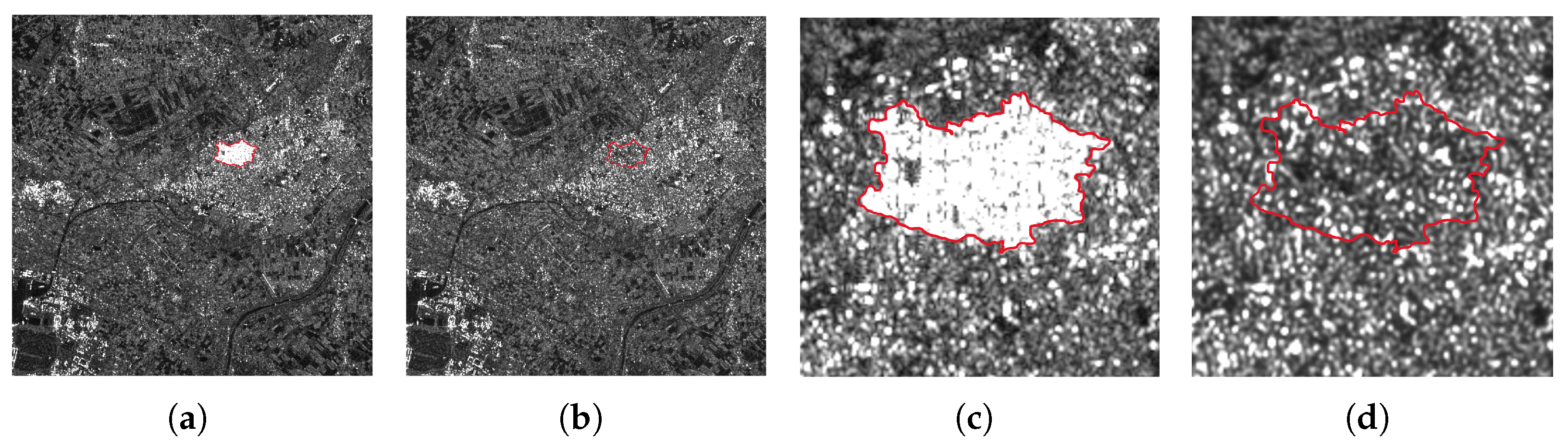
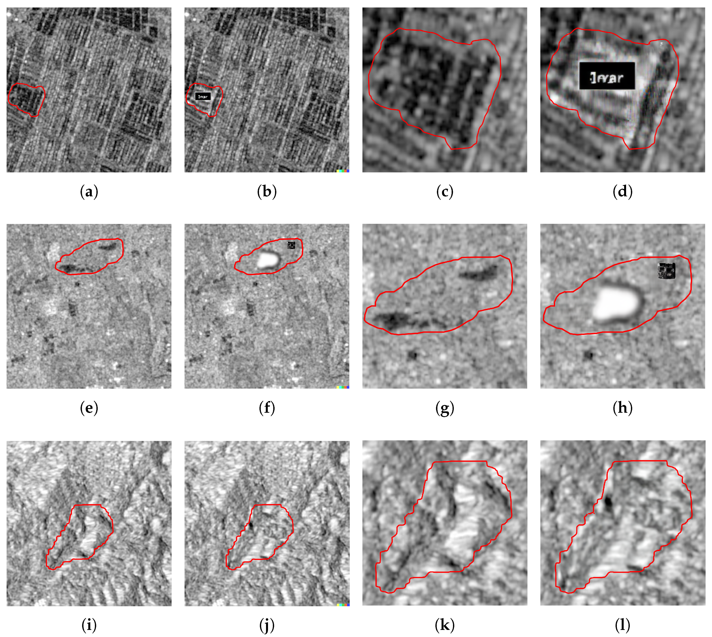
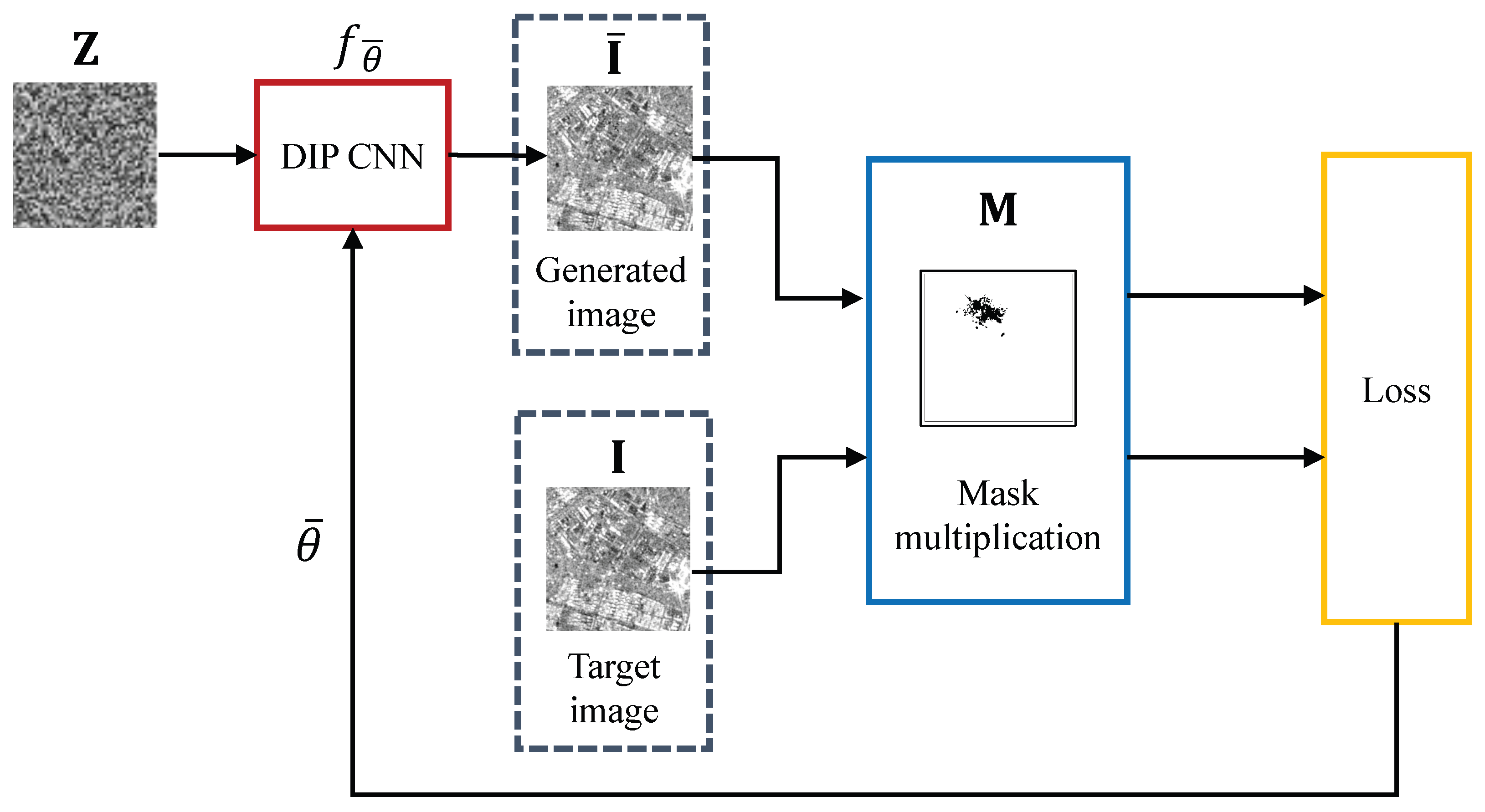
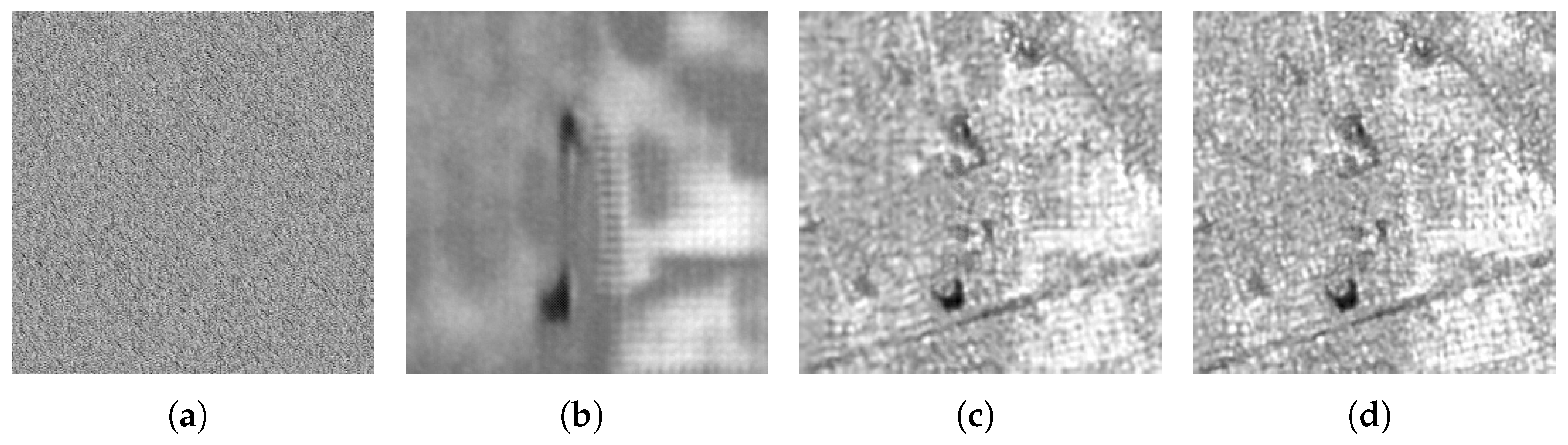
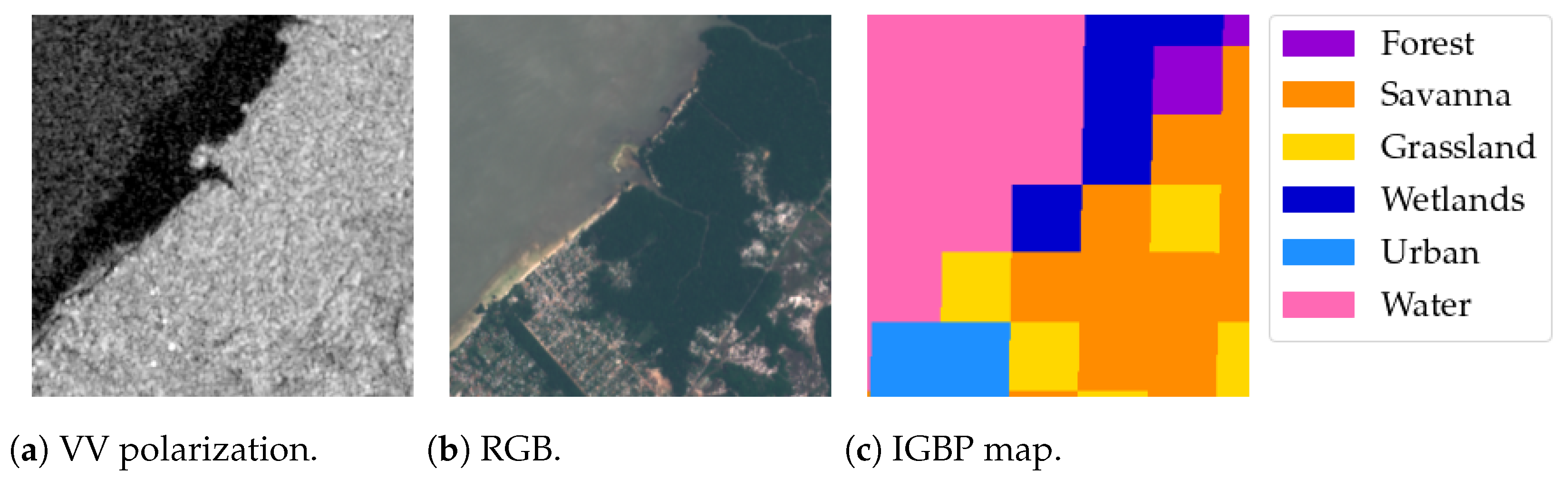
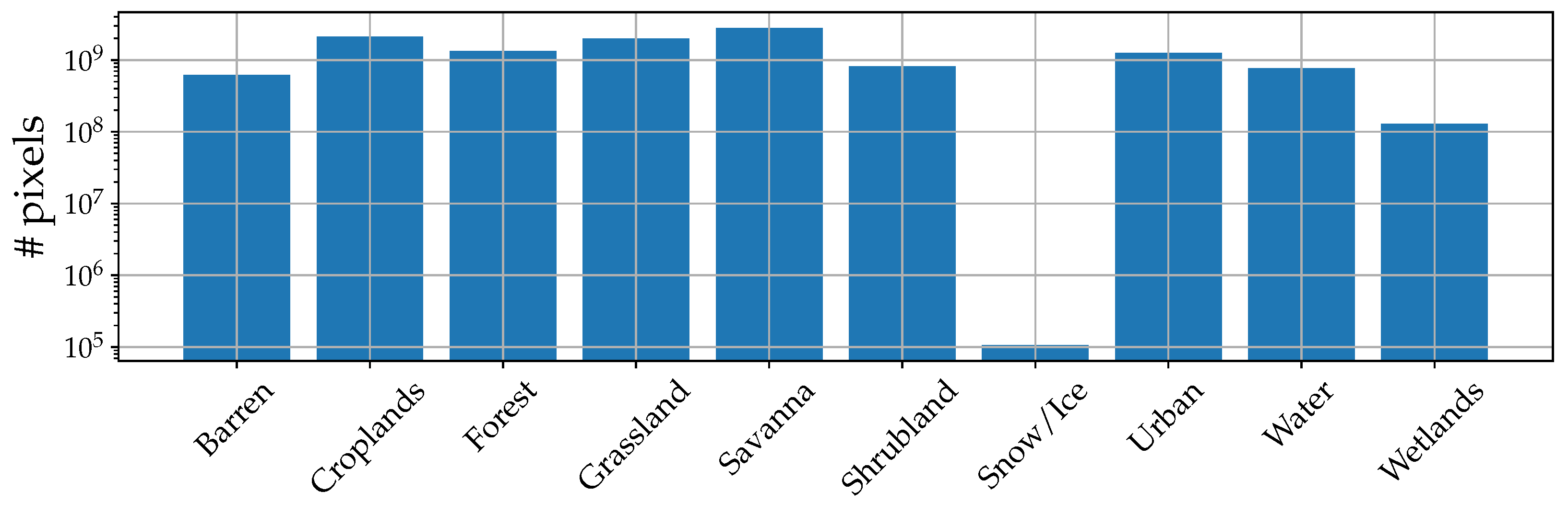
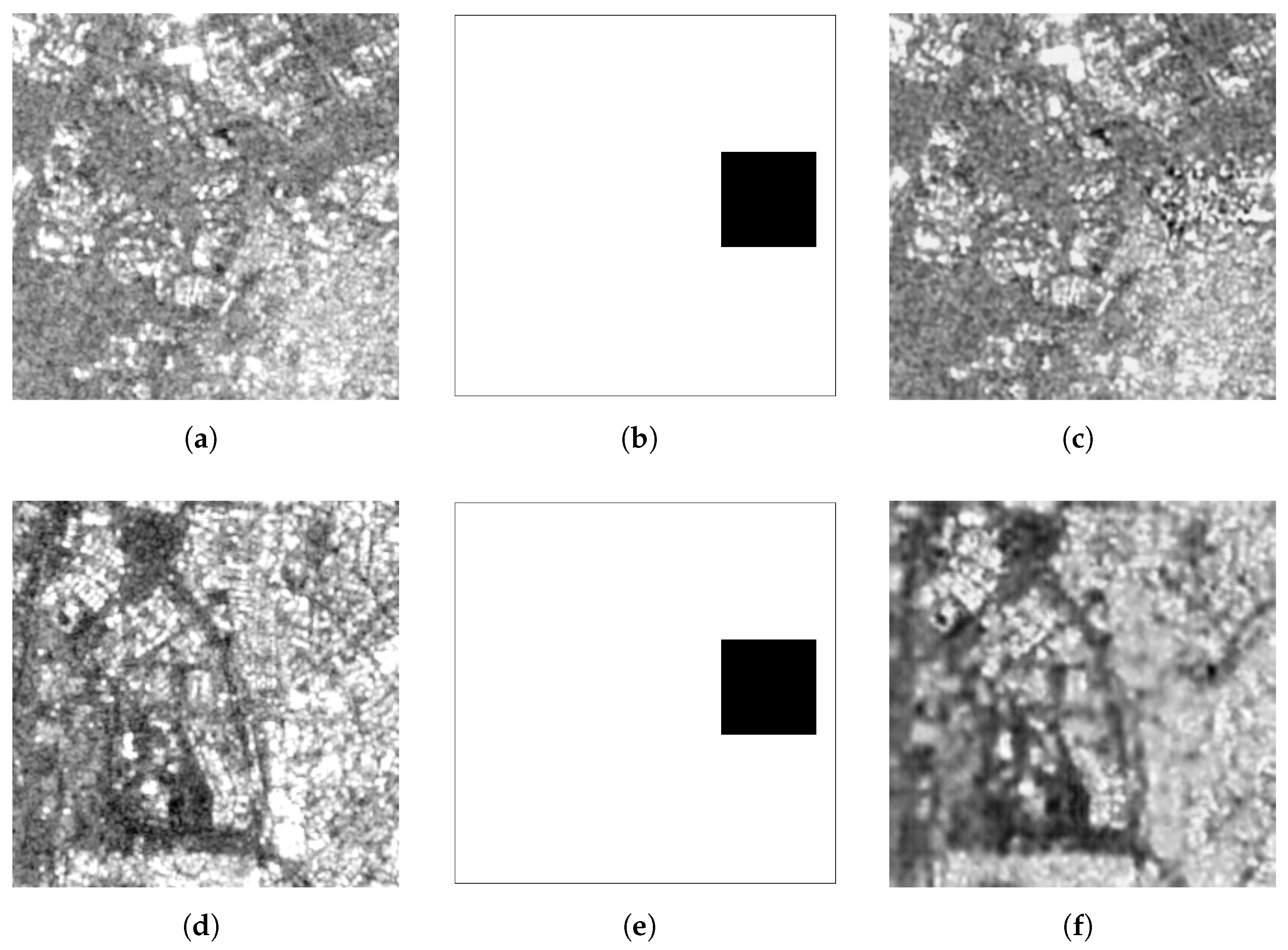
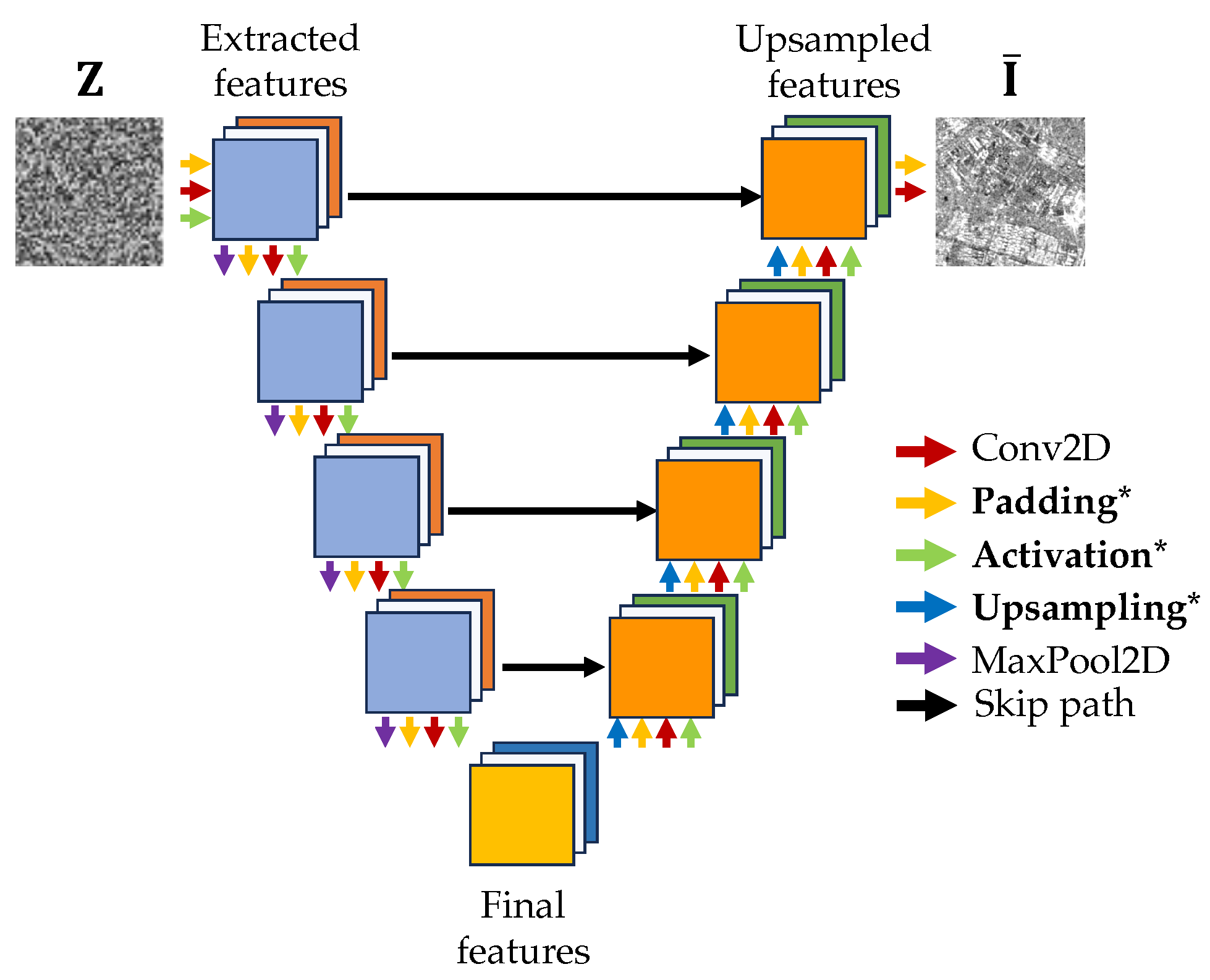
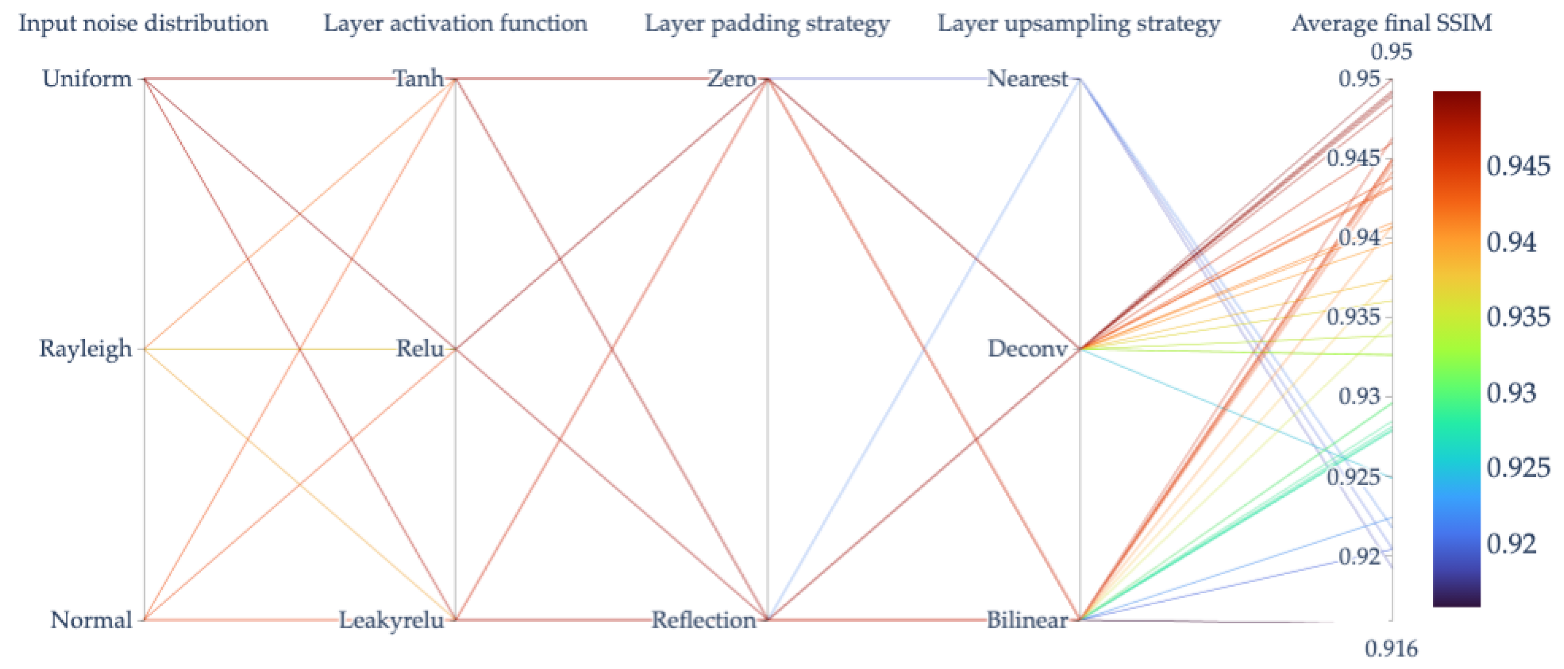
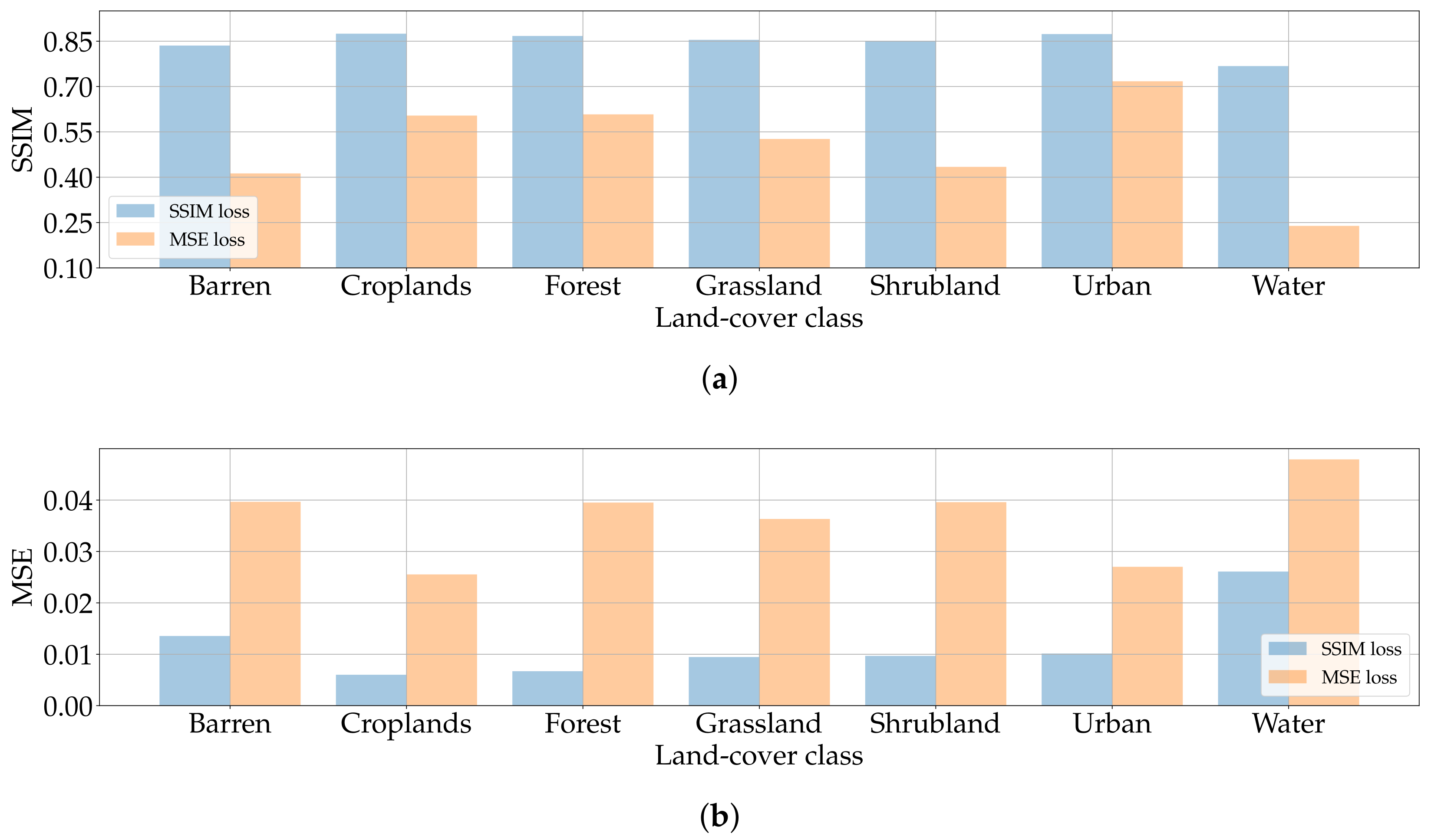
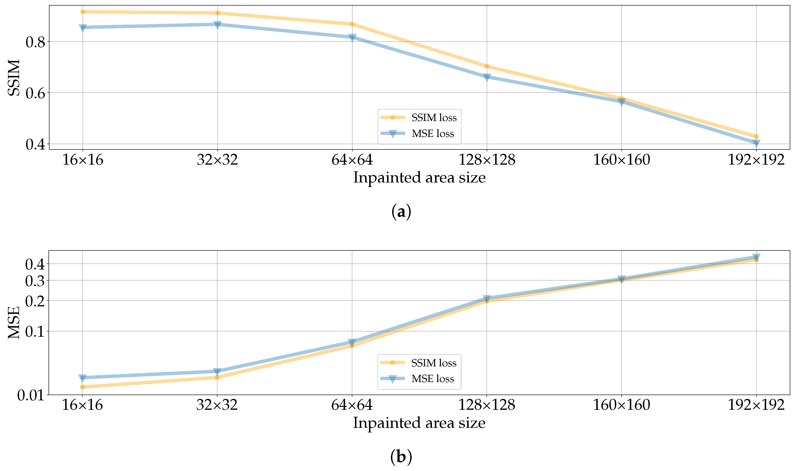
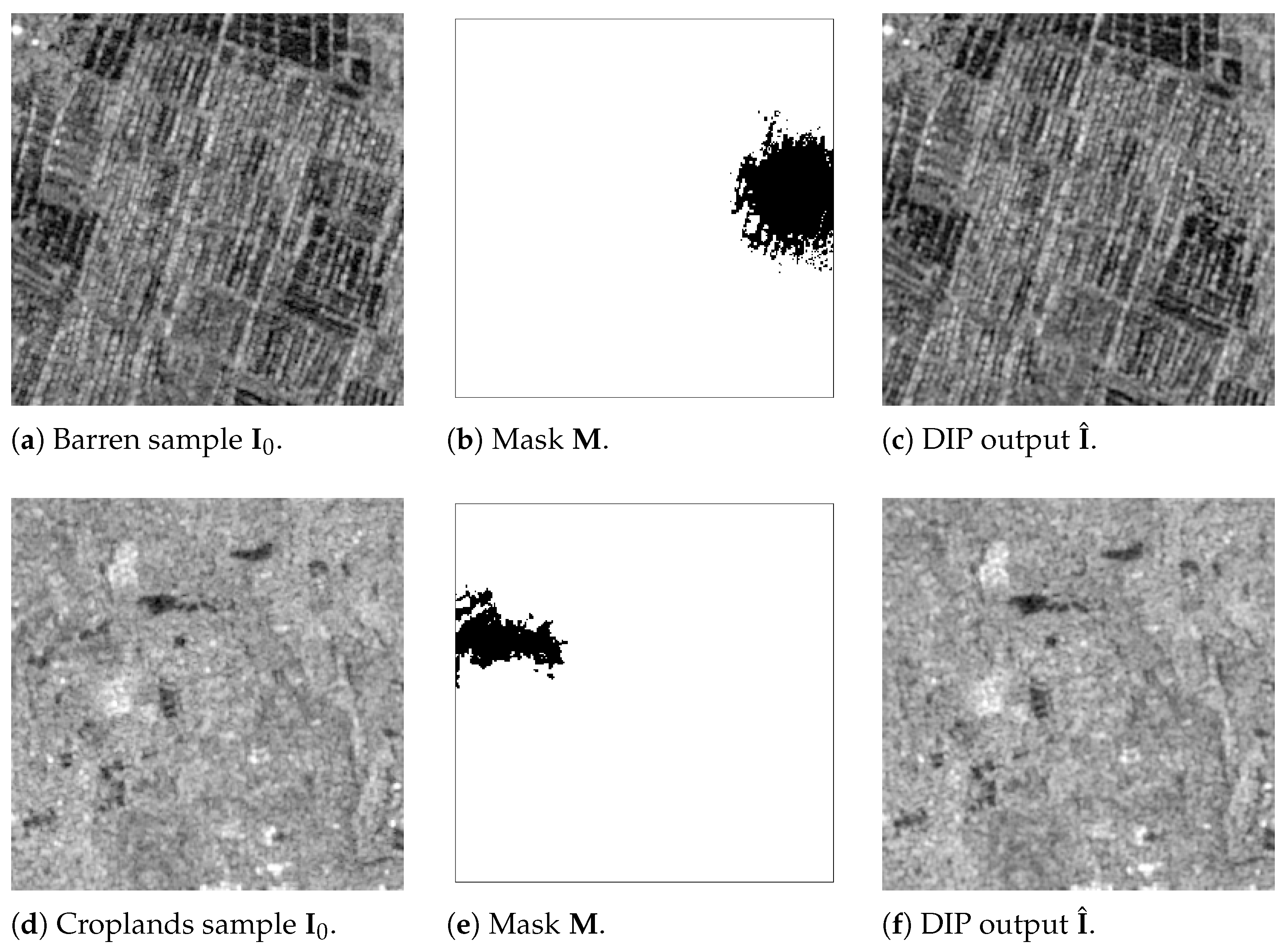
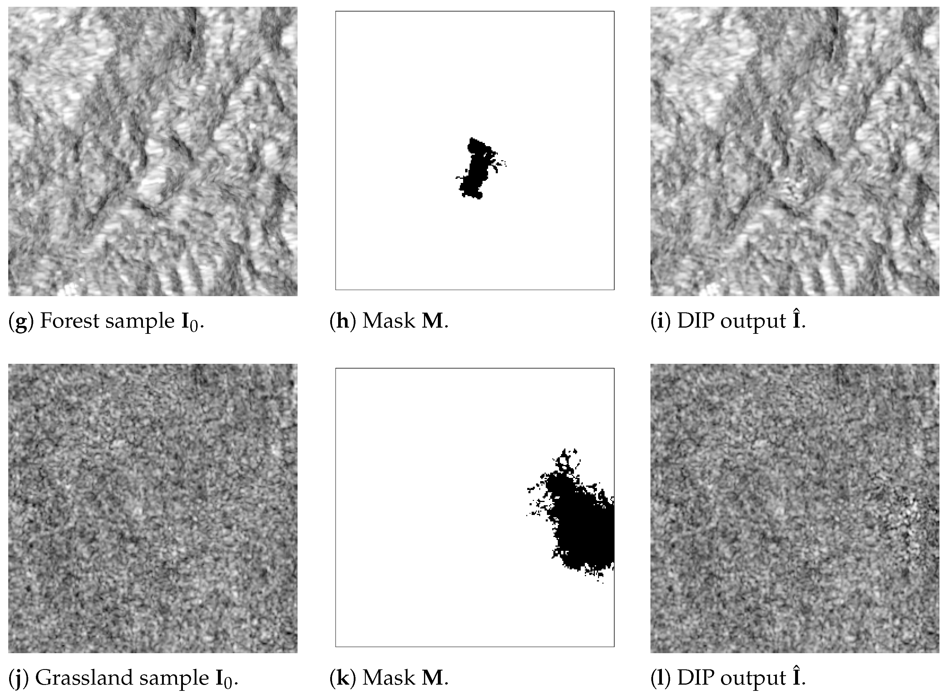
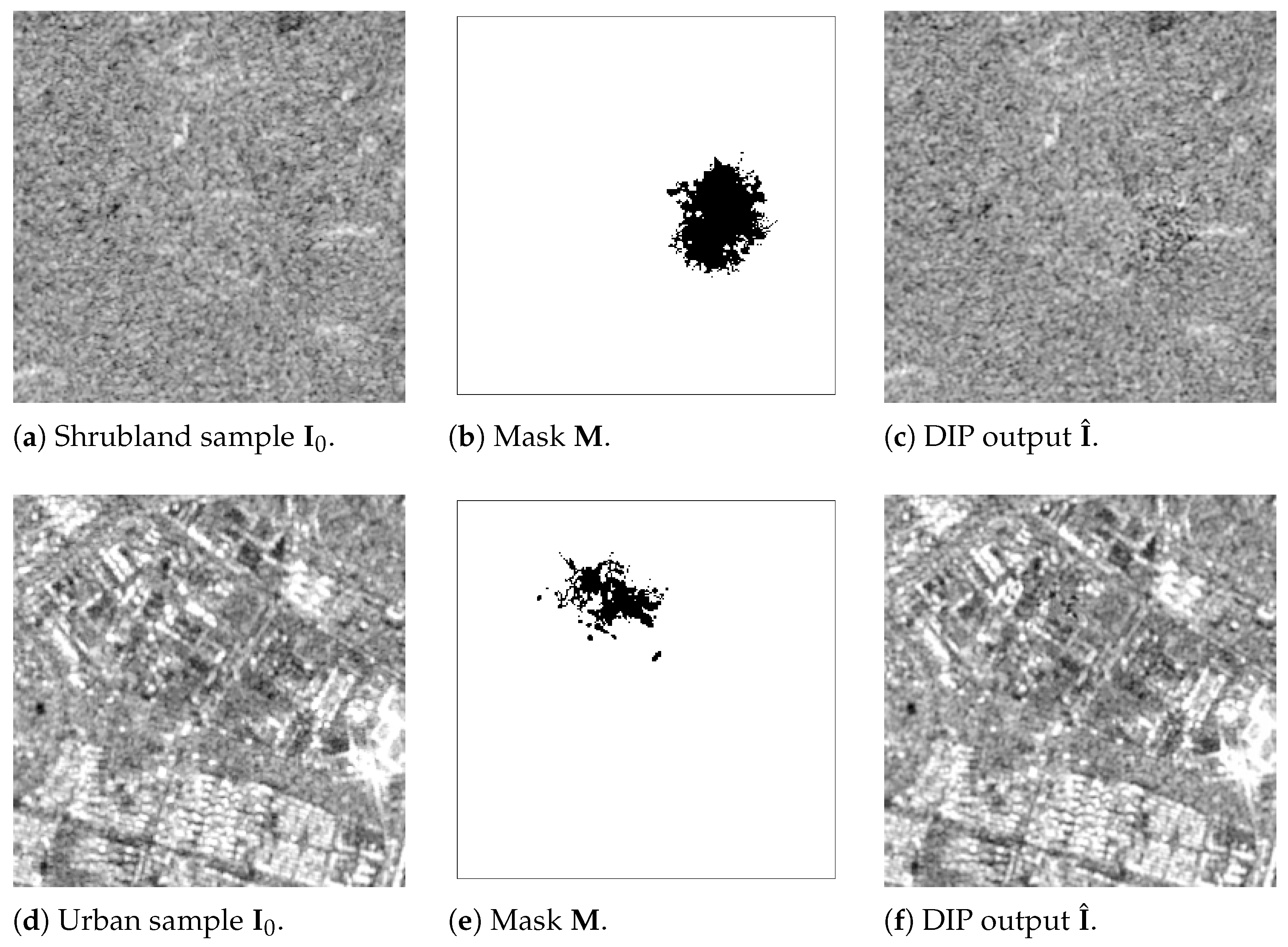
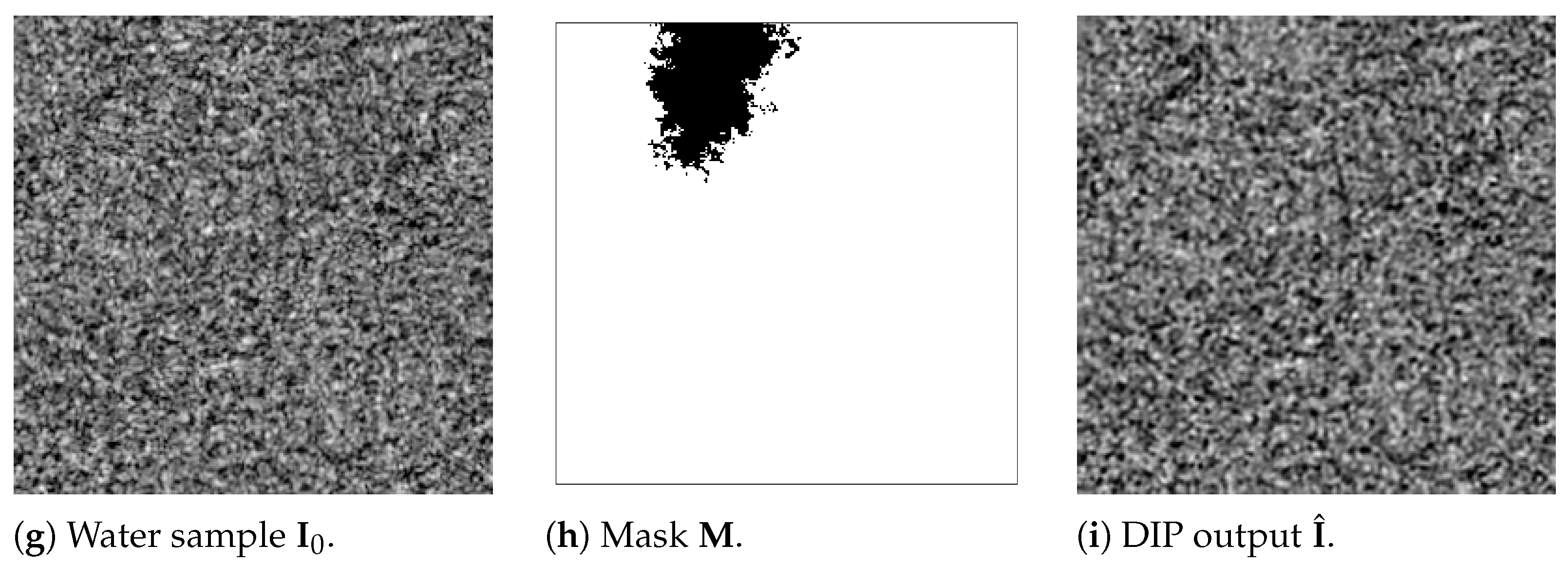
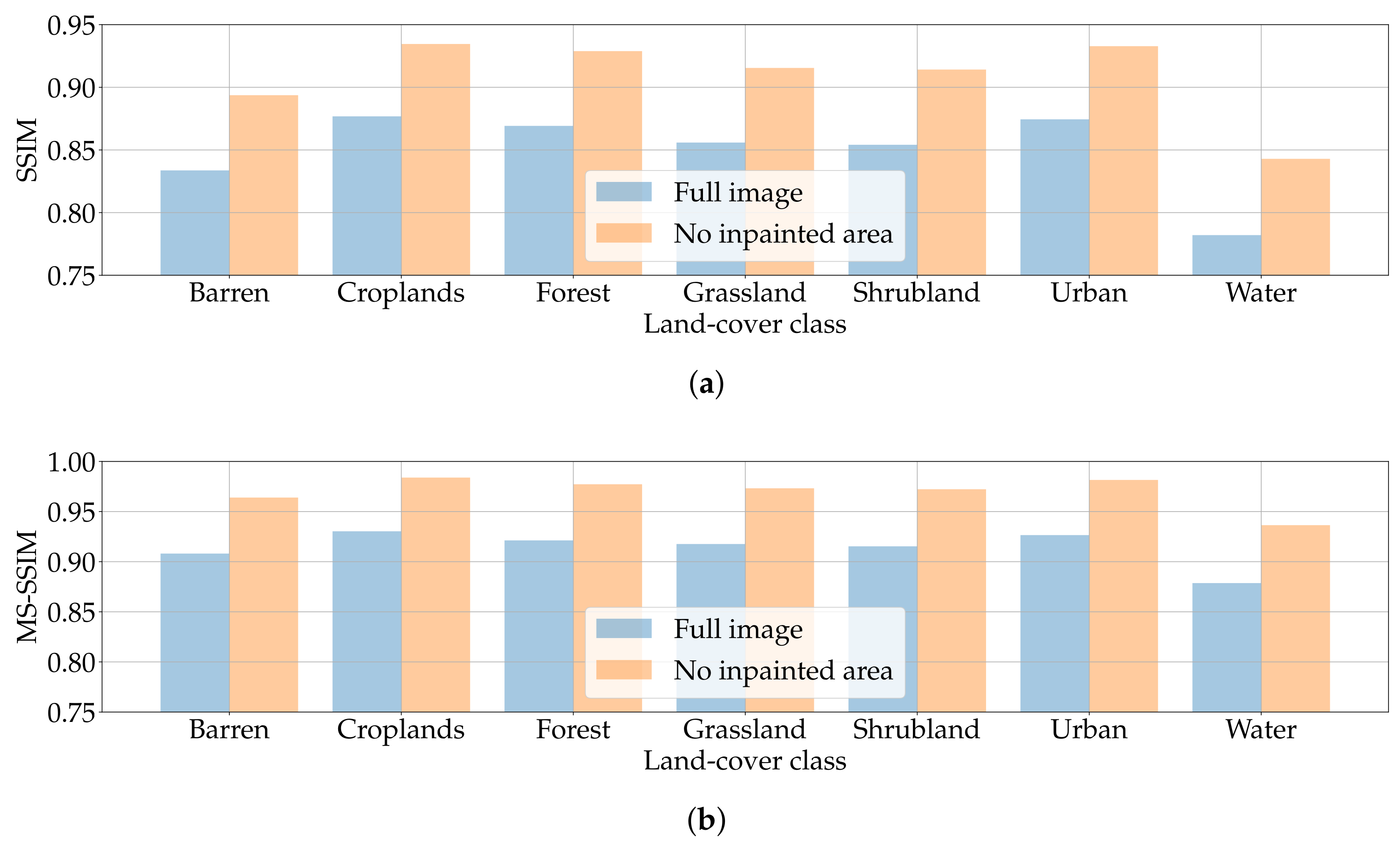
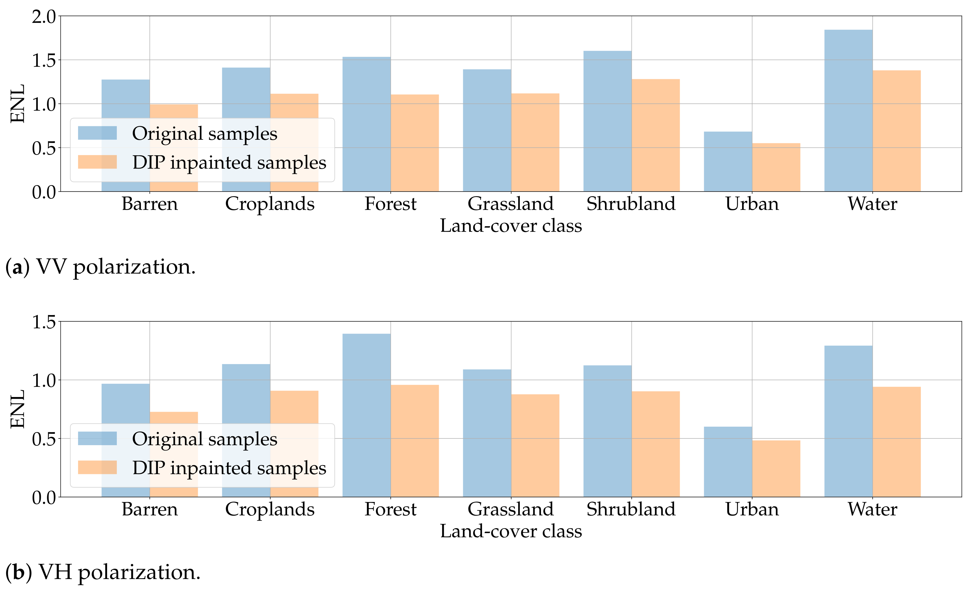
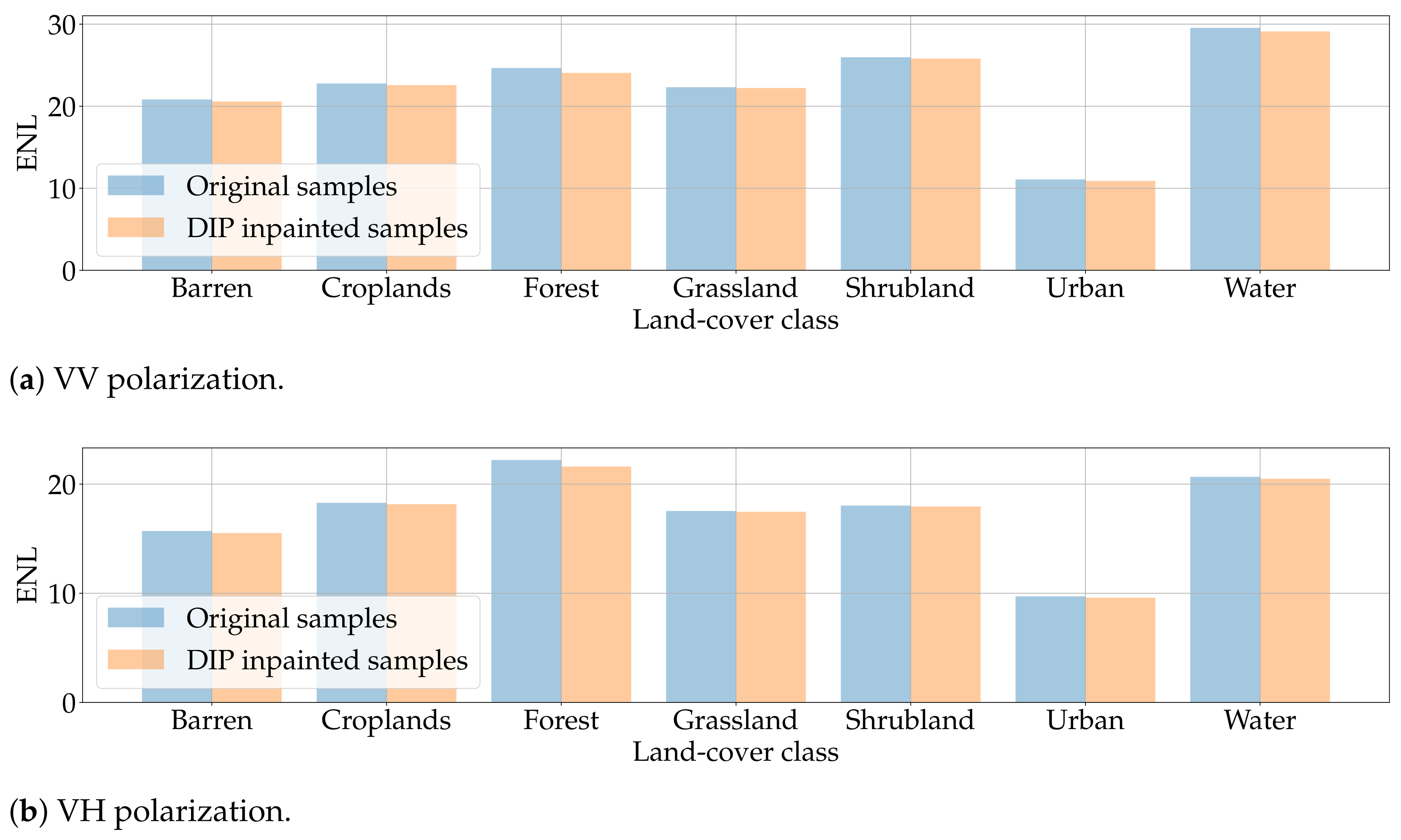
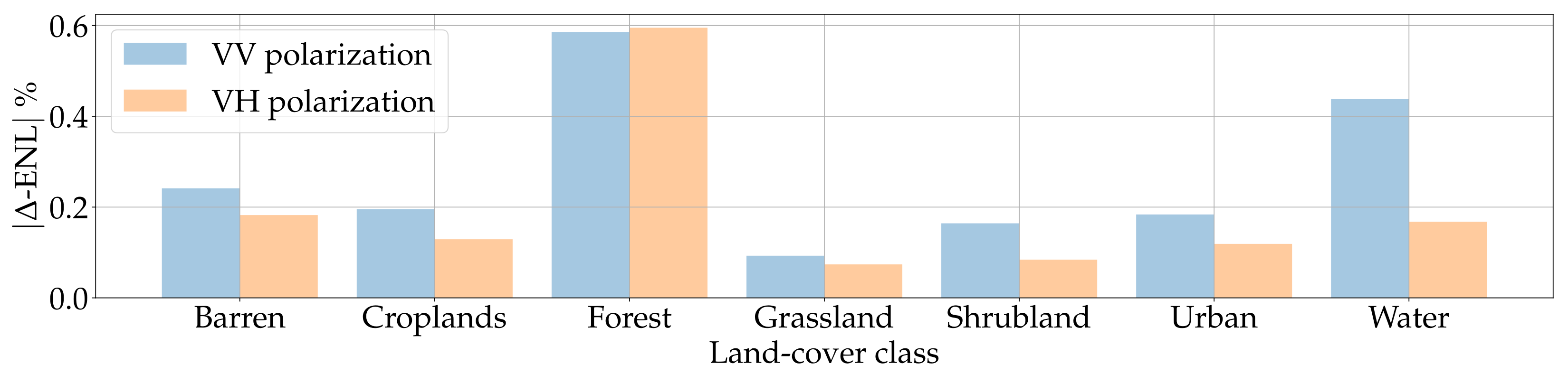
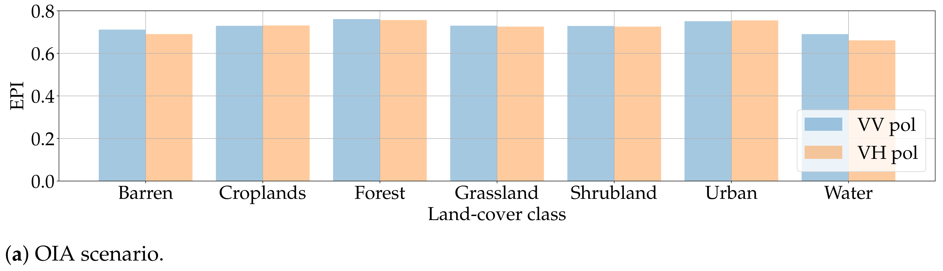
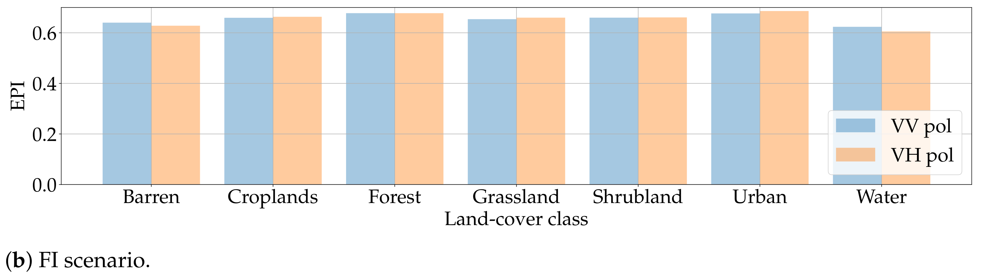
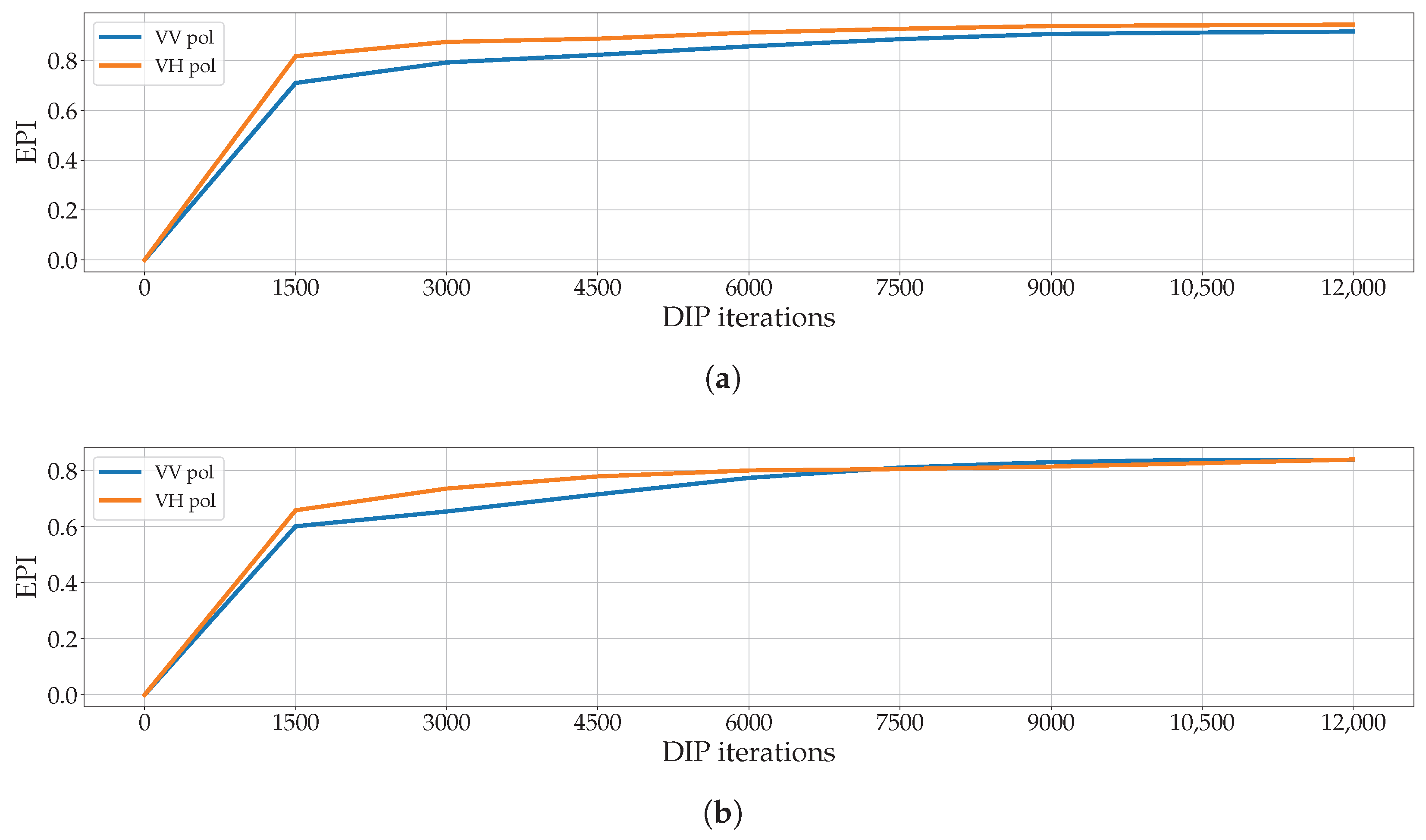
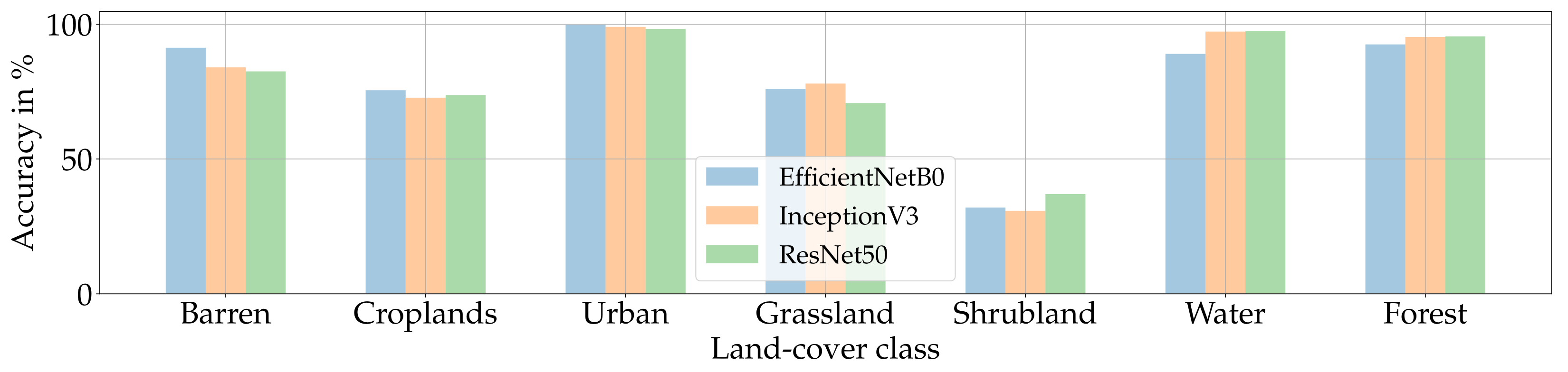
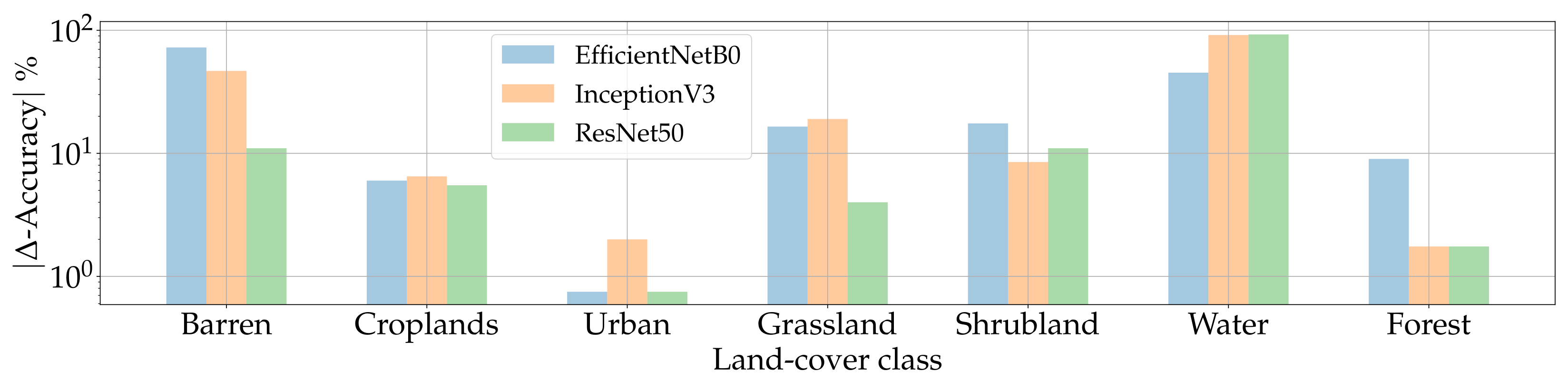
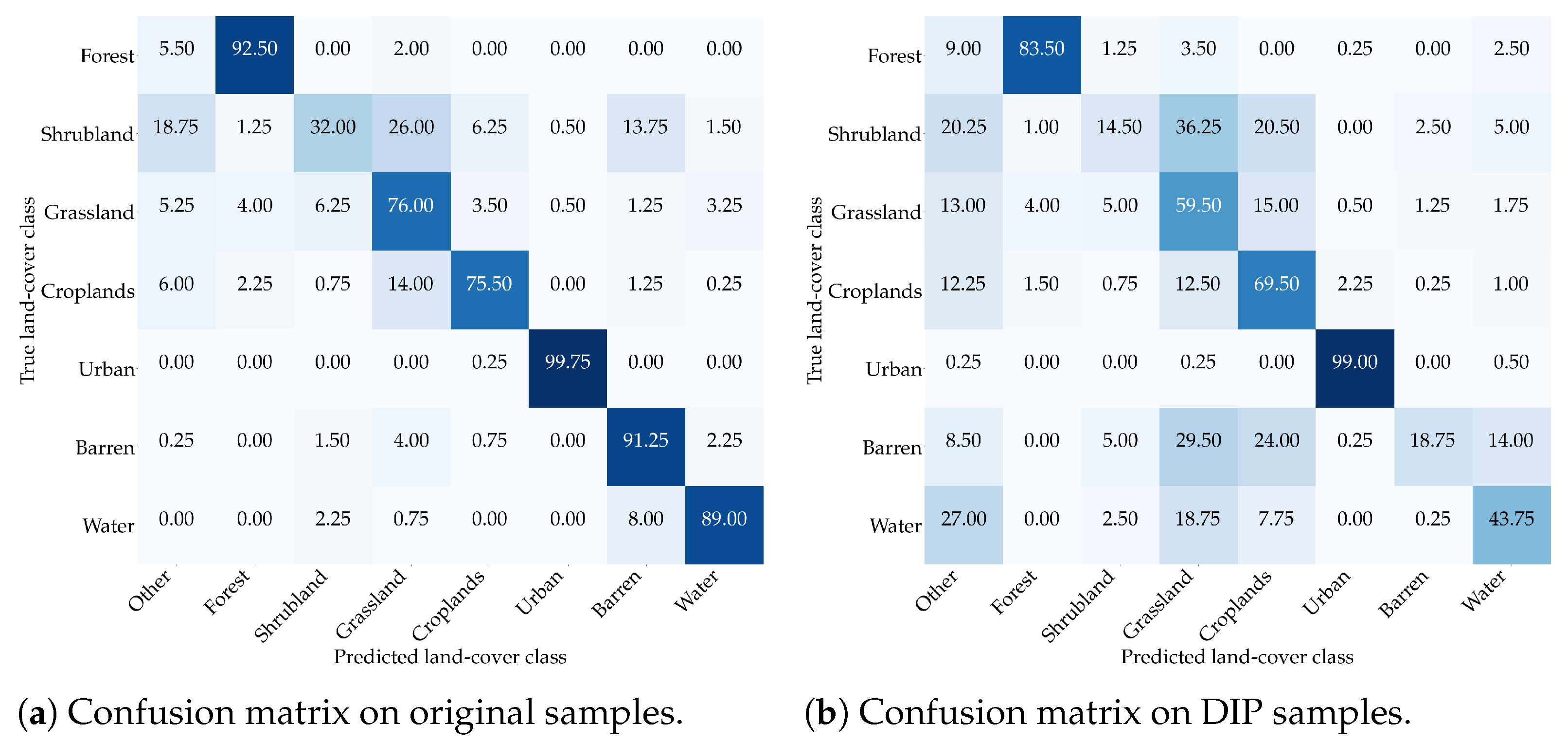
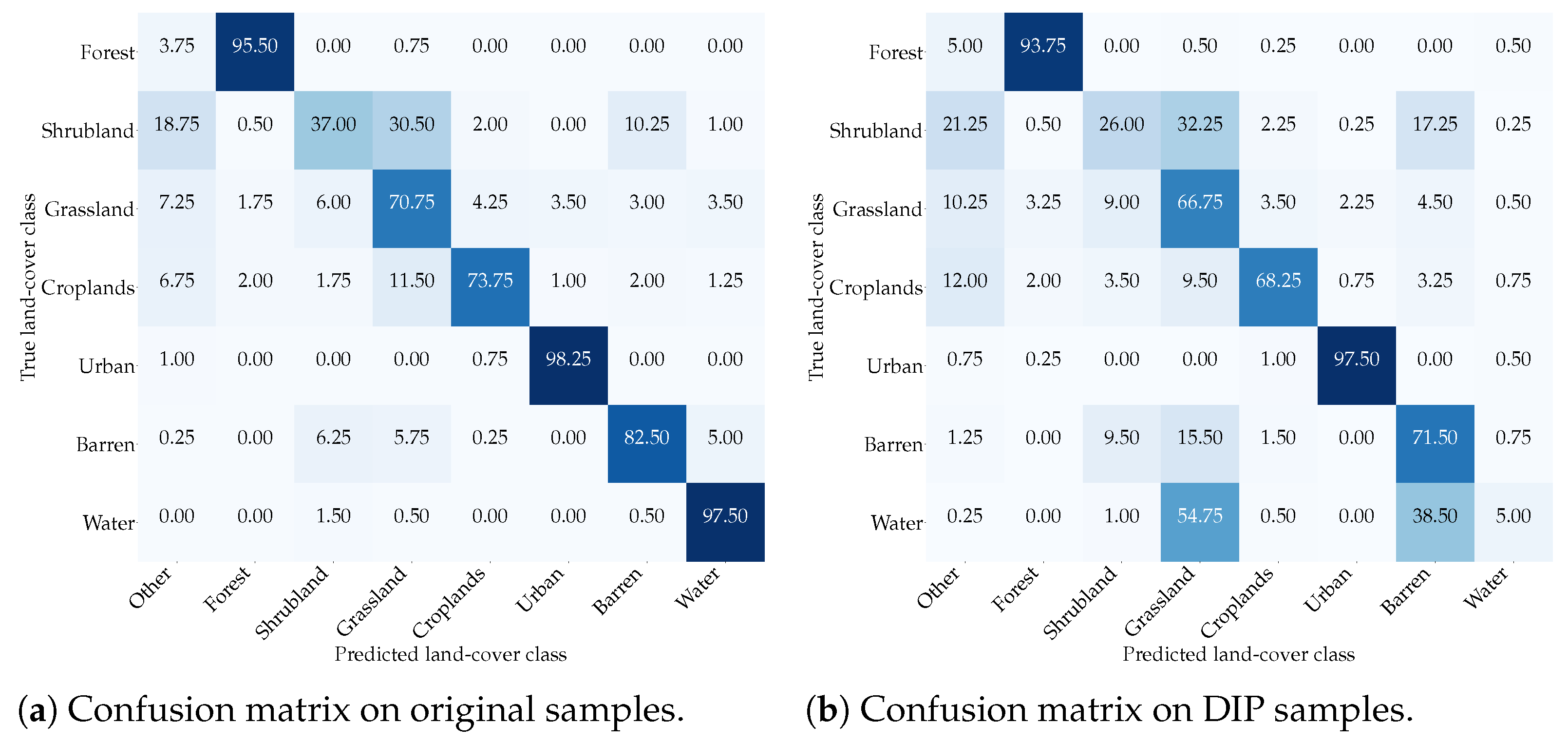
Table 1.
Selected hyperparameters for tuning the DIP technique.
| Hyperparameter Class | Parameters Values |
|---|---|
| Layer activation functions | Tanh |
| ReLU | |
| LeakyReLU | |
| Layer padding strategy | Reflection |
| Zero | |
| Layer upsampling strategy | Bilinear |
| Nearest | |
| Deconvolution | |
| Loss function | MSE |
| SSIM | |
| Input noise distribution | Gaussian |
| Rayleigh | |
| Uniform |
Disclaimer/Publisher’s Note: The statements, opinions and data contained in all publications are solely those of the individual author(s) and contributor(s) and not of MDPI and/or the editor(s). MDPI and/or the editor(s) disclaim responsibility for any injury to people or property resulting from any ideas, methods, instructions or products referred to in the content. |
© 2023 by the authors. Licensee MDPI, Basel, Switzerland. This article is an open access article distributed under the terms and conditions of the Creative Commons Attribution (CC BY) license (https://creativecommons.org/licenses/by/4.0/).
Share and Cite
MDPI and ACS Style
Cannas, E.D.; Mandelli, S.; Bestagini, P.; Tubaro, S.; Delp, E.J. Deep Image Prior Amplitude SAR Image Anonymization. Remote Sens. 2023, 15, 3750. https://doi.org/10.3390/rs15153750
AMA Style
Cannas ED, Mandelli S, Bestagini P, Tubaro S, Delp EJ. Deep Image Prior Amplitude SAR Image Anonymization. Remote Sensing. 2023; 15(15):3750. https://doi.org/10.3390/rs15153750
Chicago/Turabian StyleCannas, Edoardo Daniele, Sara Mandelli, Paolo Bestagini, Stefano Tubaro, and Edward J. Delp. 2023. "Deep Image Prior Amplitude SAR Image Anonymization" Remote Sensing 15, no. 15: 3750. https://doi.org/10.3390/rs15153750
Note that from the first issue of 2016, this journal uses article numbers instead of page numbers. See further details here.