
Compensation of Background Ionospheric Effect on L-Band Geosynchronous SAR with Fully Polarimetric Data


1
School of Aerospace Science and Technology, Xidian University, Xi’an 710071, China
2
Peng Cheng Laboratory, Shenzhen 518000, China
3
College of Information Engineering, Capital Normal University, Beijing 100048, China
*
Author to whom correspondence should be addressed.
Remote Sens. 2023, 15(15), 3746; https://doi.org/10.3390/rs15153746
Submission received: 16 May 2023
/
Revised: 18 July 2023
/
Accepted: 24 July 2023
/
Published: 27 July 2023
(This article belongs to the Section Remote Sensing Image Processing)
Abstract
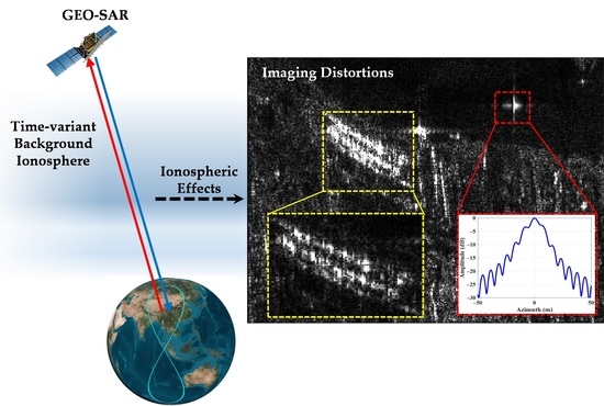
:The L-band geosynchronous synthetic aperture radar (GEO-SAR) has been widely praised for its advantages of short revisit time, wide coverage and stable backscattering information acquisition. However, due to the ultra-long integrated time, the echo will be affected by the time-variant background ionosphere, leading in particular to defocusing in the azimuth direction. Existing compensation methods suitable for low Earth orbit SAR (LEO-SAR) are based on the SAR image or the semi-focused image at the ionospheric phase screen, assuming that the ionosphere is time-frozen for a short integrated period; thus, accurate reconstruction of the time-variant characteristics for the ionosphere in GEO-SAR cannot be achieved. In this paper, a compensation method of background ionospheric effects on L-band GEO-SAR with fully polarimetric data is proposed. Considering the continuous variation of the ionosphere within the synthetic aperture, a decompression processing is proposed to reconstruct the echo by recovering the temporal sampling according to the imaging geometry. By virtue of the Faraday rotation angle, the time-variant total electron content (TEC) is accurately estimated with the reconstructed echo. Based on the established error model, the ionospheric effects are well compensated with the estimated TEC. Simulations with the real SAR data from ALOS-2 and the measured time-variant TEC from USTEC validate the effectiveness and performance of the proposed method. The impacts from thermal noise and polarimetric calibration error are also quantitatively analyzed. From this, the error thresholds are given to guarantee compensation accuracy, namely 18.96 dB for SNR, −15.63 dB for crosstalk and −1.02 dB to 0.31 dB for the amplitude of the channel imbalance, and the argument of the channel imbalance is suggested to be maintained as close to zero as possible.
1. Introduction
L-band fully polarimetric (FP) synthetic aperture radar (SAR) has superior advantages in penetration and temporal coherence, which has been widely used in geological surveys and biomass measurements, such as the Phased Array-type L-band SAR (PALSAR) of Advanced Land Observation Satellite (ALOS) series [1,2,3]. Geosynchronous synthetic aperture radar (GEO-SAR) could achieve much shorter revisit time (even continuous observation for a given area) and greatly wider coverage (thousands of kilometers) compared to the traditional low Earth orbit SAR (LEO-SAR) systems, thereby providing much richer information [4]. To date, several assumed L-band GEO-SAR missions have been proven to retrieve relatively stable backscattering information from the target and plan to realize measurements of water data, snow mass monitoring and mapping of terrain deformation [5,6,7,8].
Meanwhile, the L-band echo is known to be more sensitive to the ionosphere during propagation, which will lead to serious distortions for radar images [9,10]. According to the variation and distribution of the ionosphere, two kinds of typical structures are recognized, i.e., the background ionosphere and irregularity [11]. The former represents the large-scale and slow-variant structure of electrons which is always regarded as time-frozen for LEO-SAR system in a short observation. In addition, the fluctuant part known as irregularity could introduce ionospheric scintillation to the signal, but it is time- and region-restricted [12], which can be partly avoided by orbit design, such as the dawn–dusk orbit of the BIOMASS mission [13]. Thus, from the view of imaging, ionospheric effects on the LEO-SAR signal are mainly about group delay and range dispersion due to the background ionosphere [11]. The corresponding compensation methods, such as maximum contrast and multi-look autofocus, have also been proposed to solve these problems [14,15].
However, for the GEO-SAR system, the ionosphere cannot be treated as time-frozen for more than 1 min of integrated time and larger than 1000 km of swath [16]. Therefore, defocusing and positioning errors occur due to the phase advance and time delay related with the time-variant total electron content (TEC), especially for the azimuth signal [17,18]. To solve this problem, there are two main kinds of ways for compensation at present. The first kind realizes ionospheric compensation with TEC inversion through difference frequency. Typically, Hobbs et al. proposed a TEC measuring method based on dual-frequency signals, which can be used to compensate for the ionospheric effects [19]. However, the bandwidth requirement for this method is quite high (to improve compensation accuracy) [19]. The other kind of compensation uses autofocus processing, just as Long et al. have systematically researched the compensation of ionospheric effects for the GEO-SAR and put forward a compensation method based on phase grade autofocus (PGA) [20]. However, PGA relies on the strong scattering point in the image, which fails for the homogeneous scene [21,22]. Guarnieri et al. prove the effectiveness of PGA when dealing with atmospheric phase distortion but specifically for wet tropospheric interference [23]. Furthermore, Li et al. use contrast optimization autofocus (COA) to compensate for the time-variant ionospheric effect on GEO-SAR focusing, but the requirement of a strong target in the image is still indispensable [24]. Hu and Ding have applied autofocus processing based on minimum entropy to compensate for the ionospheric effects on GEO-SAR imaging, but Hu mainly concentrates on scintillation compensation [25], and Ding’s method considers the different types of imaging errors as a whole including the ionosphere [26]. In addition, Zhang et al. rely on the optimization processing of coherent character to solve background ionospheric phase distortion [27]. As the coherent character of the target is used during processing, the applicable conditions are quite strict, where the block processing and the isolate-prominent point target are necessary. Therefore, there are still some limitations to the existing methods to well compensate for the time-variant ionospheric effects on GEO-SAR systems.
In this article, a compensation method of background ionospheric effects on GEO-SAR with fully polarimetric data is proposed. The background ionospheric effects on the GEO-SAR signal are discussed in Section 2. Based on the transmission characteristic of electromagnetic waves in the ionosphere, the error model of time delay and phase advance is established. Considering the ultra-long integrated time of GEO-SAR, the specific ionospheric effect with time-variant TEC is specifically analyzed for both azimuth and range signals. In Section 3, the compensation method of background ionospheric effects based on FR estimation is proposed. In order to separate the time-variant TEC within the synthetic aperture, decompression processing is conducted considering the imaging geometry. Then, the corresponding phase error at each pulse is compensated for through time-variant FR angle estimation. Simulations and analyses with real SAR data from ALOS-2 and time-variant TEC from USTEC are shown in Section 4. The performance and problems of the proposed method and previous related studies are discussed in detail in Section 5. Our follow-up research is also presented in this section. Finally, conclusions are drawn in Section 6.
2. Background Ionospheric Effects on the GEO-SAR Signal
2.1. Properties of Electromagnetic Wave Transmission in the Ionosphere
As a typical kind of plasma, the group refractive index of the electromagnetic wave in the ionosphere can be expressed by the approximation of the Appleton–Hartree expression as [11]
where f is the frequency of the electromagnetic waves, and fN is the plasma frequency as [11]
where e is the charge of an electron, me is the electron mass, ε0 is the permittivity of vacuum, and Ne is the electron density.
Based on the group refractive index in (1), the time delay caused by the ionosphere compared with a vacuum is given by [28]
where c is the speed of light, K is a constant of 40.28 m3/s2, and TEC is the total electron content along the propagation path with the unit of TECU (1 TECU = 1016 m−2).
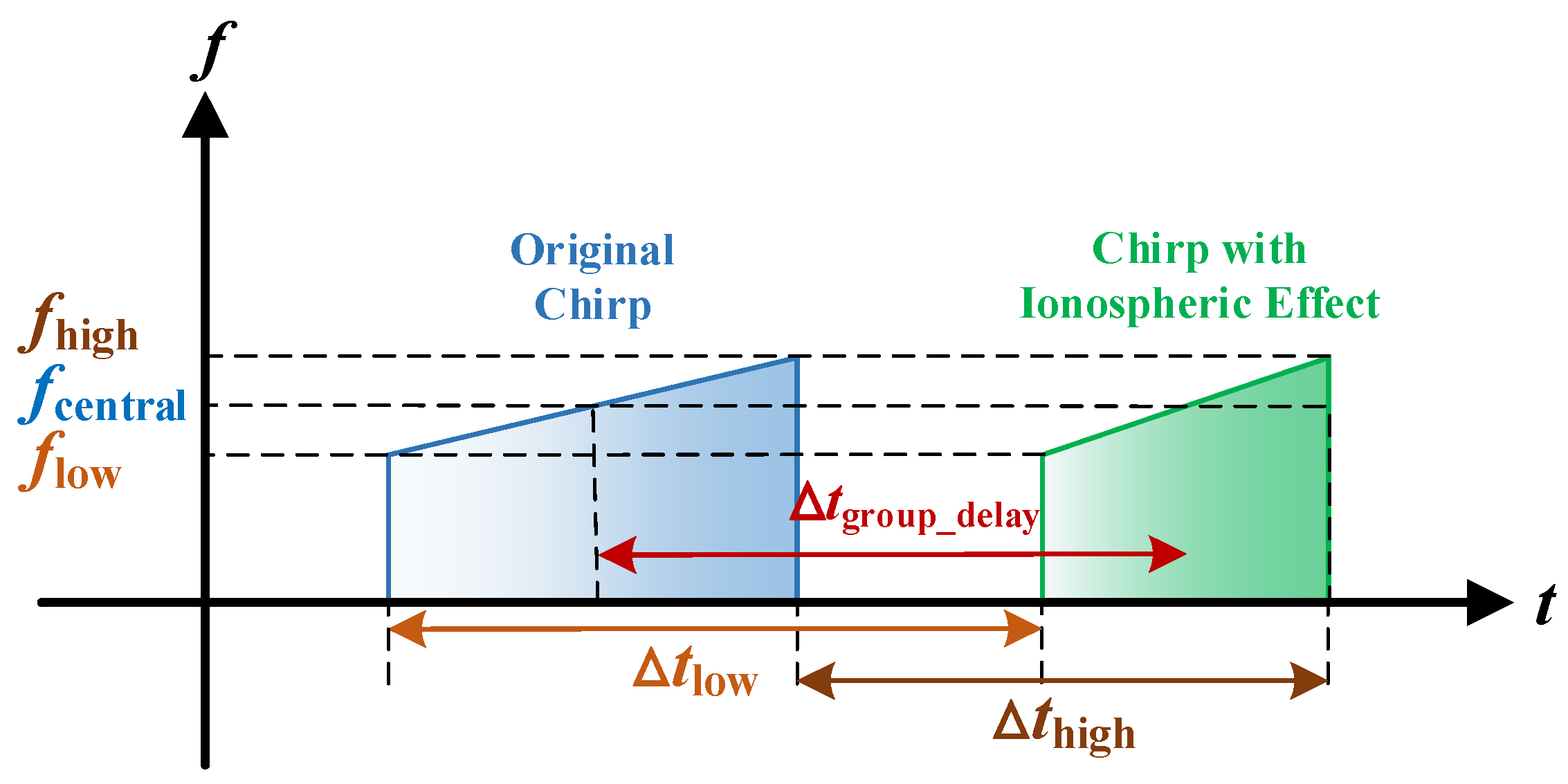
Considering the time delay at the carrier frequency, it could represent the delay of the signal envelope, which is known as the group delay (marked with the red arrow line in Figure 1). Since the time delay Δt(f) is related to the frequency f, different frequency components of the chirp pulse are delayed differently, resulting in a change in the chirp rate, which is the root of the defocusing caused by the ionosphere. Accordingly, the affected chirp rate b′ is derived as (4) according to the relationship between the bandwidth and the changed pulse length.
where Bw is the bandwidth, Tp is the pulse length, fc is the carrier frequency, and Δthigh and Δtlow are the time delays at the highest and lowest frequencies within the bandwidth, respectively.
In addition to the time delay, the phase characteristic of the radar signal is also changed during the two-way propagation, which is known as the phase advance. It can be calculated according to the time delay Δt(f) as [29]
From the view of frequency domain, the Taylor expansion of the additional phase in (5) is derived as (neglecting the higher-order terms)
The first-order term in (6) represents the time delay corresponding to (3), and the second-order term will cause a mismatch during the matched filtering, leading to the defocusing of the chirp signal [15]. Thus, the impacts of ionospheric effects on the electromagnetic wave, including the time delay and the phase advance, could be unified as the additional phase error in (5), which conforms to the properties of the ionosphere as the dispersion medium.
2.2. Error Model of Time-Variant Background Ionospheric Effects on the GEO-SAR Signal
The ideal-point echo signal of the GEO-SAR system is traditionally expressed as [10]
where Wr(*) and Wa(*) are the envelope functions of the range and azimuth, respectively, t and τ are the azimuth and range time, respectively, b is the chirp rate of range signal, λ is the wavelength, and R(t) is the slant range.
After the two-way propagation through the ionosphere, the affected echo is derived as below, according to the error model shown in (5). Here, TEC(t) is related to the azimuth time t, which reflects the time-variant characteristic of the ionosphere.
where fr is the frequency of the range signal.
In order to facilitate ascertaining the impacts of the background ionosphere on GEO-SAR imaging more clearly, the Taylor expansion of the ionospheric phase in (8) is derived as (neglecting the higher-order terms)
For the range signal, the pulse width of the existing SAR system is always tens of microseconds, during which the change in TEC could be neglected. Thus, the first-order phase in (9), corresponding to the time delay at each sampling time, will cause the group delay for the range signal (see Figure 1); the second-order phase brings the error to the chirp rate leading to the defocusing of the range signal, which is called dispersion. That is, the background ionosphere TEC(t) at each azimuth sampling time introduces the frequency-dependent phase to the range signal. According to the properties of Fourier transform, the corresponding offset and defocusing should happen after matched filtering.
Usually, the range quadratic phase error (QPE) is used to evaluate the impact on focusing for range signal, which is derived as (10) according to (9).
Considering the allowable uncompensated QPE of π/4 [30], the corresponding TEC(t) should be at least 16 TECU for 1 m resolution and 145 TECU for 3 m resolution, so that the range signal will be affected. According to the statistical analysis and release data of the ionosphere, the vertical TEC is generally less than 120 TECU [31,32]. Thus, the impact of the background ionosphere on range signal imaging is quite weak given the general state of the ionosphere for L-band SAR with a resolution more than 3 m; meanwhile, for the L-band systems with a higher resolution (such as LuTan-1 [33]), the effects on range signal should be compensated.
On the other hand, the azimuth signal is contaminated with the additional time-related phase at each sampling time according to (9). Comparing with the range signal, the change in the TEC(t) is quite large within the integrated time of azimuth signal especially for GEO-SAR. With the change rate of TEC(t), different orders of the phase error will lead to distortions of the azimuth signal, among which the first-order term causes the overall offset, and the second and higher orders cause defocusing [16]. The related error analysis and numerical simulations have been discussed by many scholars, particularly in [16,17,24].
3. Compensation of Background Ionospheric Effects Based on FR Estimation
3.1. Faraday Rotation Estimation with FP SAR Data
In magnetized plasma, the polarization plane of the electromagnetic wave is rotated by Ω for the linearly polarized wave when propagating through the ionosphere, which is known as a Faraday rotation (FR) [34]. The rotation angle is
where KΩ is a constant of 2.365 × 10⁴ A⋅m2/kg, B is the magnetic flux density, and ψ is the angle the wave makes with the Earth’s magnetic field.
Traditionally, the FR effect on the SAR signal depends on the polarization mode. For the linearly FP SAR system specifically, the signal of each polarimetric channel will be contaminated by the others according to (12) [35].
where S** and M** are the true and measured scattering components of each polarimetric channel, respectively (the subscript “**” represents HH, HV, VH or VV).
For now, several FR estimation methods have been proposed [36,37,38], among which Bickel and Bates’s method shows better performance [39]. The core idea of this method is to estimate the FR with the difference of cross-polarized channels in circular-polarized bases Z12 and Z21 as
Then, the FR angle is estimated as
where <*> represents the smoothing operation to reduce the influence from the thermal noise, and arg(*) gives the angle of its complex-valued argument.
3.2. Compensation Method
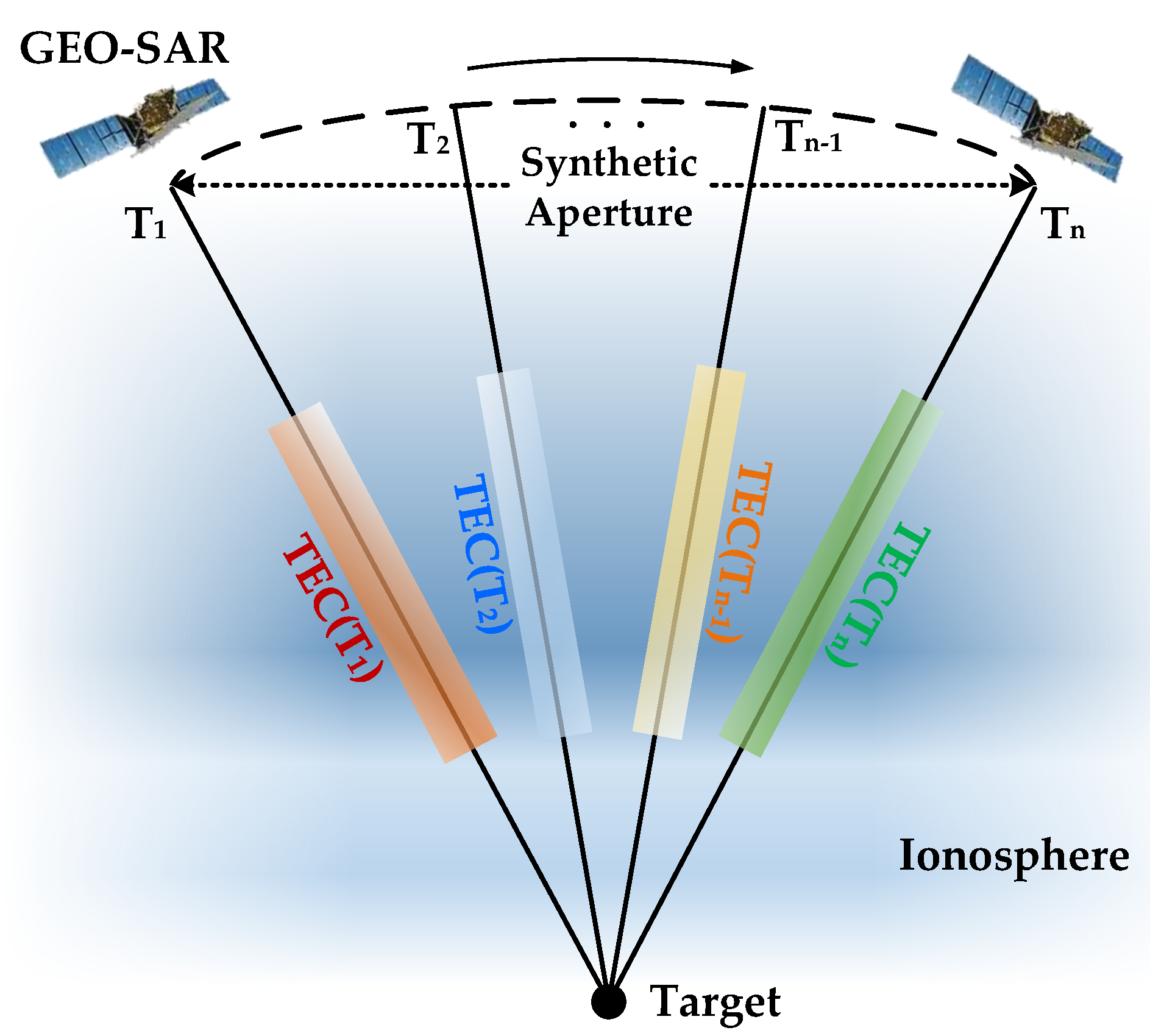
According to the analysis in Section 2.2, the state of the background ionosphere between adjacent radar pulses changes with time due to the quite low pulse repetition frequency (PRF) and the ultra-long integrated time of GEO-SAR. Specifically, the time-variant background ionosphere imports the errors at each pulse sampling time with TEC(t) (shown in Figure 2).
Considering the time variation of TEC(t), the Faraday rotation angle caused by the background ionosphere changes with time, or more exactly, azimuth sampling time t (see (15)).
Combining (8) and (15), which are both related with TEC(t), if the TEC(t) is estimated accurately through the Faraday rotation angle, the ionospheric phase error could be well compensated. Inspired by this, the fully polarimetric GEO-SAR data are firstly used to estimate the time-variant Faraday rotation angle at each azimuth sampling time. Then, the time-variant ionospheric phase can be obtained from the estimated TEC(t) according to (5), which is derived from the FR estimation in (14). The estimated time-variant ionospheric phase is written as (16). Finally, the imaging distortion is compensated with the azimuth echo at range frequency domain based on the model in (8).
However, the synthesized affected SAR image cannot be used to estimate the FR directly. This is because the FR angle caused by the time-variant TEC is also compressed during focusing, which loses the information of temporal sampling. Therefore, the image should be decompressed to reconstruct the echo in azimuth firstly, so as to recover the physical distribution of the time-variant ionospheric errors.
Different from the traditional semi-focused processing of scintillation compensation for LEO-SAR [40], the GEO-SAR decompression should recover the original echo instead of the approximate echo at the altitude of the phase screen, because the phase screen model only fits for the “frozen in” ionosphere with “spatial and not temporal variations” [15]. The integrated information at each time point within the synthetic aperture is reset to its original acquisition time for the specific target, which is equivalent to a kind of reverse imaging processing. Based on the mature research studies about GEO-SAR imaging [41,42,43], this reverse imaging processing could be realized from the time or frequency domains [44].
Taking the reverse imaging processing at the frequency domain, for example, the specific processing of decompression is to obtain the frequency spectrum in azimuth with Fourier transform firstly as
Then, the decompressed frequency spectrum of the azimuth echo is obtained with multiplying by the decompressed phase as shown below, which refers to the azimuth compression in [45].
The azimuth echo is reconstructed with inverse Fourier transform of (18) as
Based on the reconstructed azimuth echo, the time-variant FR angle is estimated with each sampling signal according to (13) and (14) as
where and represents the cross-polarized signals with (13).
The corresponding time-variant ionospheric phase is obtained from (16) as
Because the ionospheric phase is frequency-dependent, the compensation should be done in the frequency domain of range signal as
Then, the compensated echo is derived with inverse Fourier transform as
Finally, the re-compressed processing is conducted to obtain the compensated image by removing the decompressed factor in the Doppler domain.
It should be noted that during the reconstruction of the azimuth echo, the signal-to-noise Ratio (SNR) of the radar signal will decrease, which leads to a loss of accuracy for FR estimation. In order to overcome this problem, the number of looks should be increased properly to guarantee the accuracy for FR estimation.
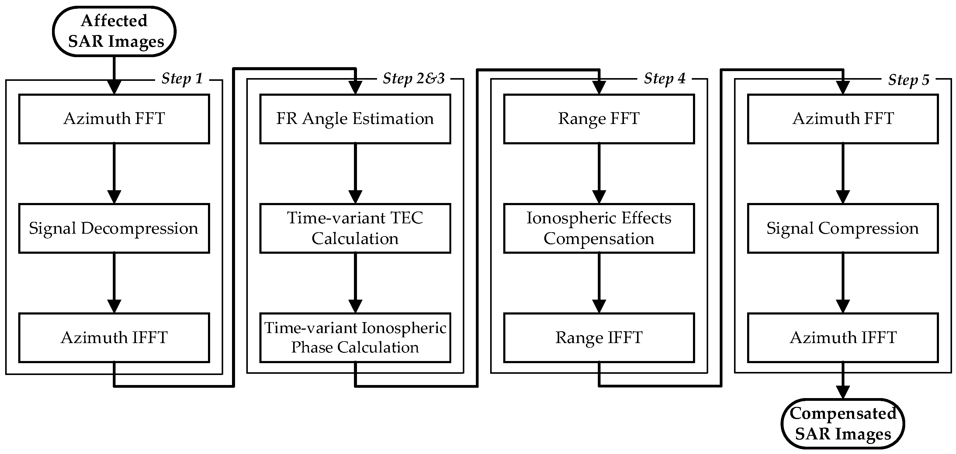
The complete compensating flow is summarized as follows:
- Reconstruction of the azimuth echo with decompression for each polarimetric channel;
- Estimation of the FR angle at each sampling time with FP signals;
- Calculation of the time-variant ionospheric phase with estimated from the FR angle;
- Compensation for the ionospheric effects with the estimated time-variant phase;
- Re-compression of the azimuth echo.
The corresponding compensating flow diagram is shown in Figure 3.
4. Experiments and Analyses
4.1. Simulation Based on Real FP SAR and TEC Data
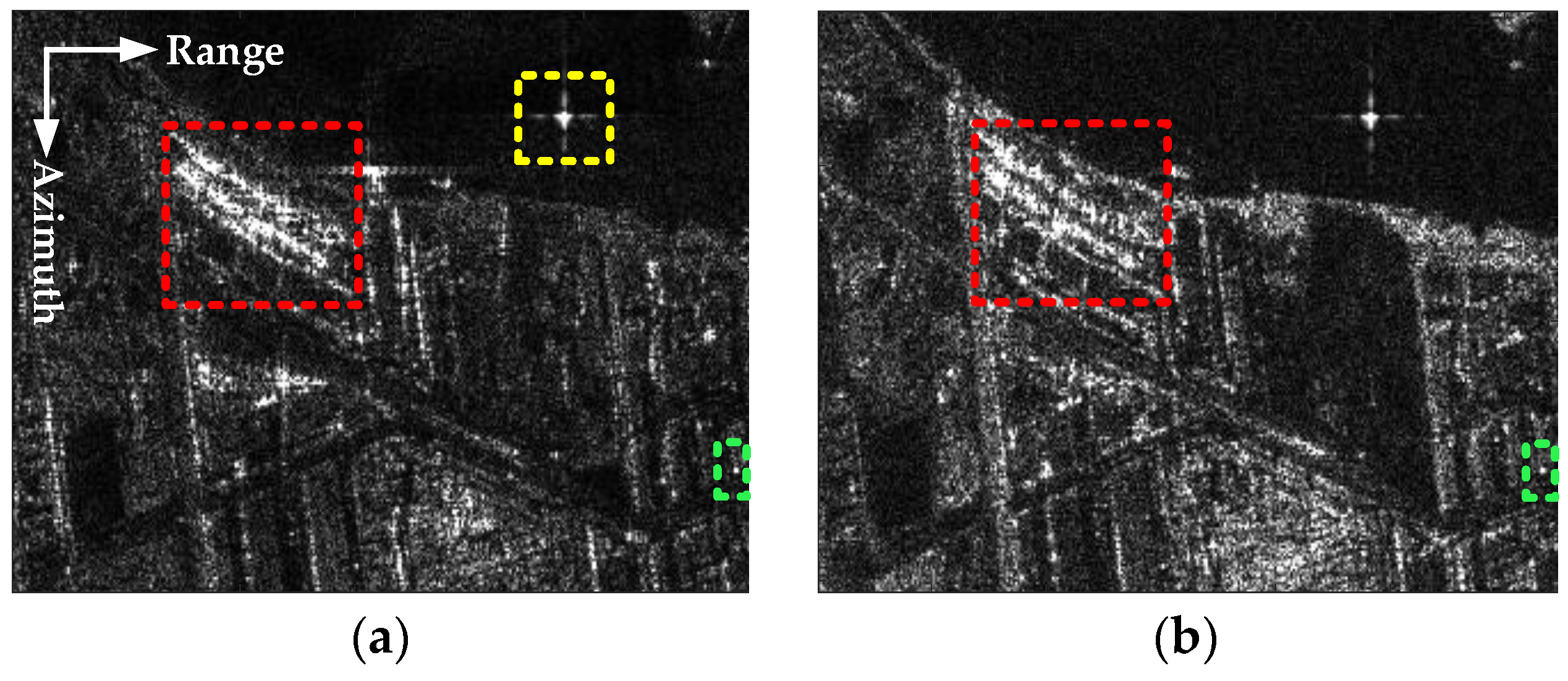
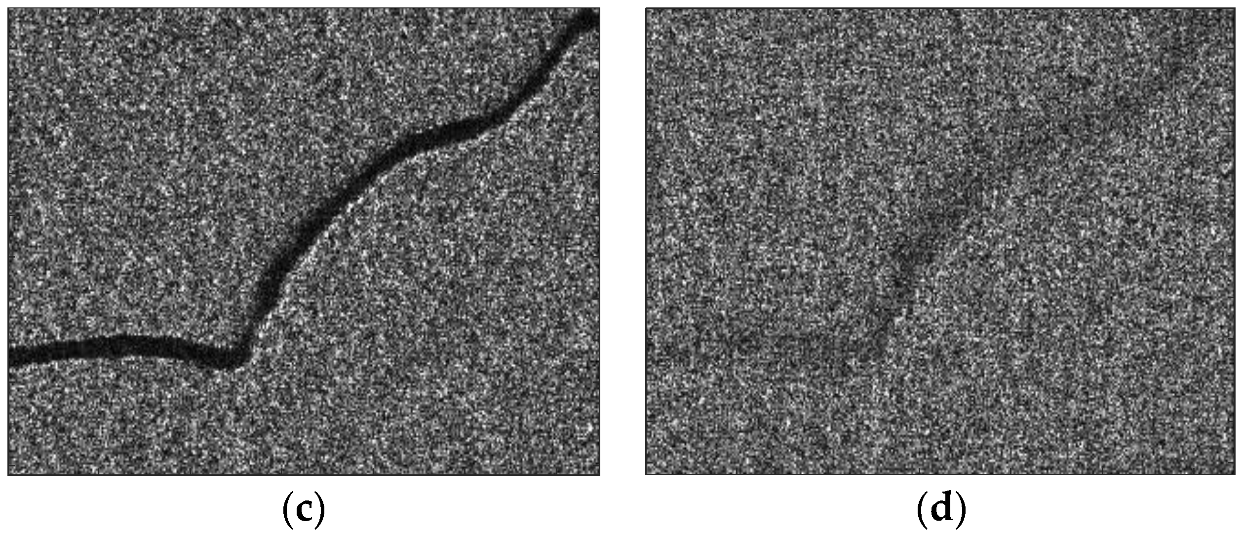
According to the geometric properties of GEO-SAR imaging, the FP SAR images are simulated using the real SAR data from ALOS-2 with 3 m resolution as the backscattering coefficients. With the parameters in Table 1, the original FP images are simulated under two kinds of scenes (heterogeneous and homogeneous, respectively), which are shown in Figure 4. The original ionospheric effects in ALOS-2 data are compensated, and the cross-polarized channels are equalized before simulation to eliminate the effects of the original ionospheric effects and polarimetric calibration errors.
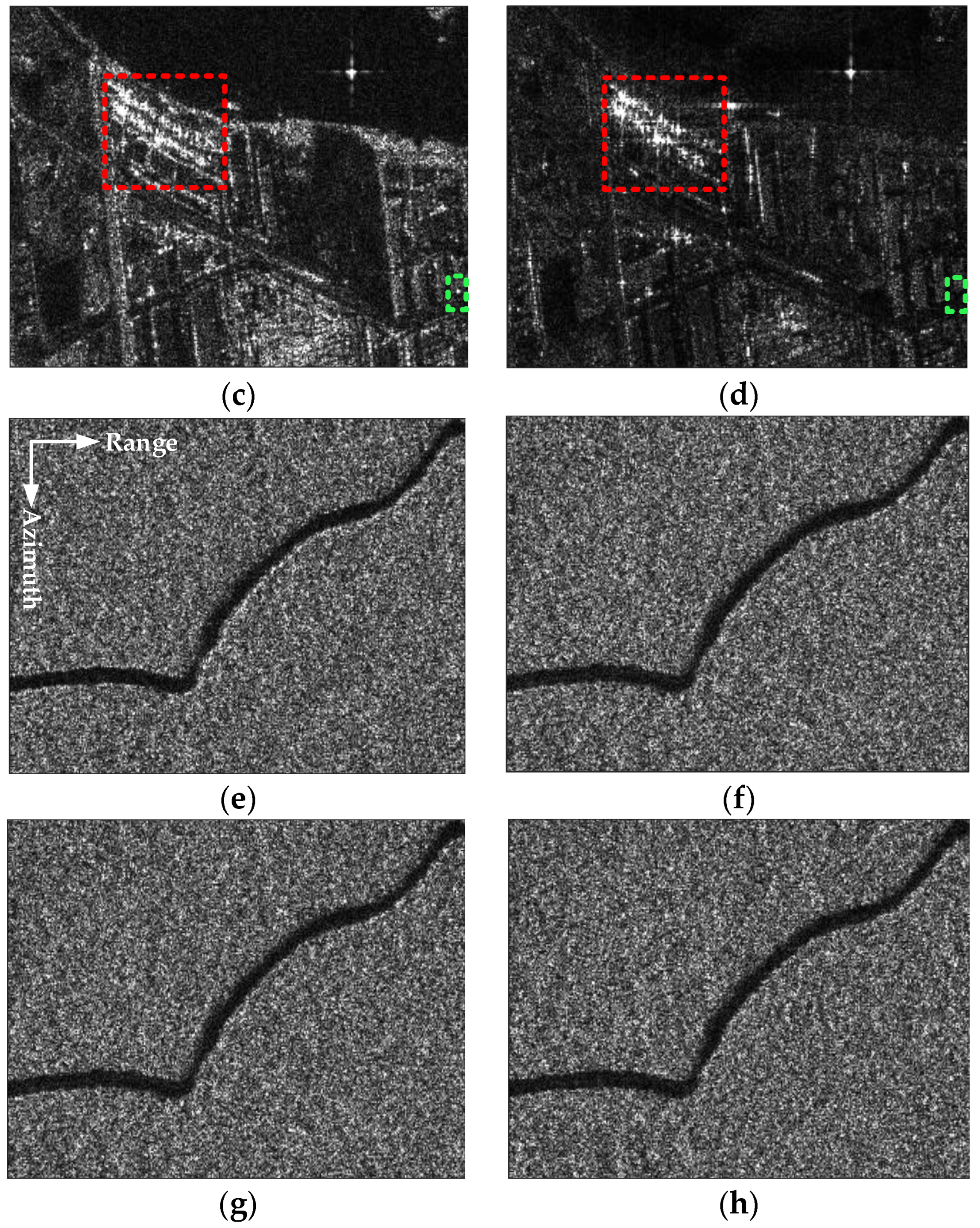
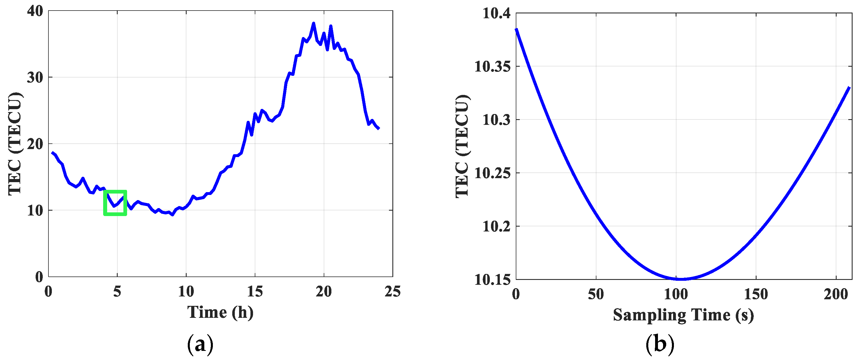
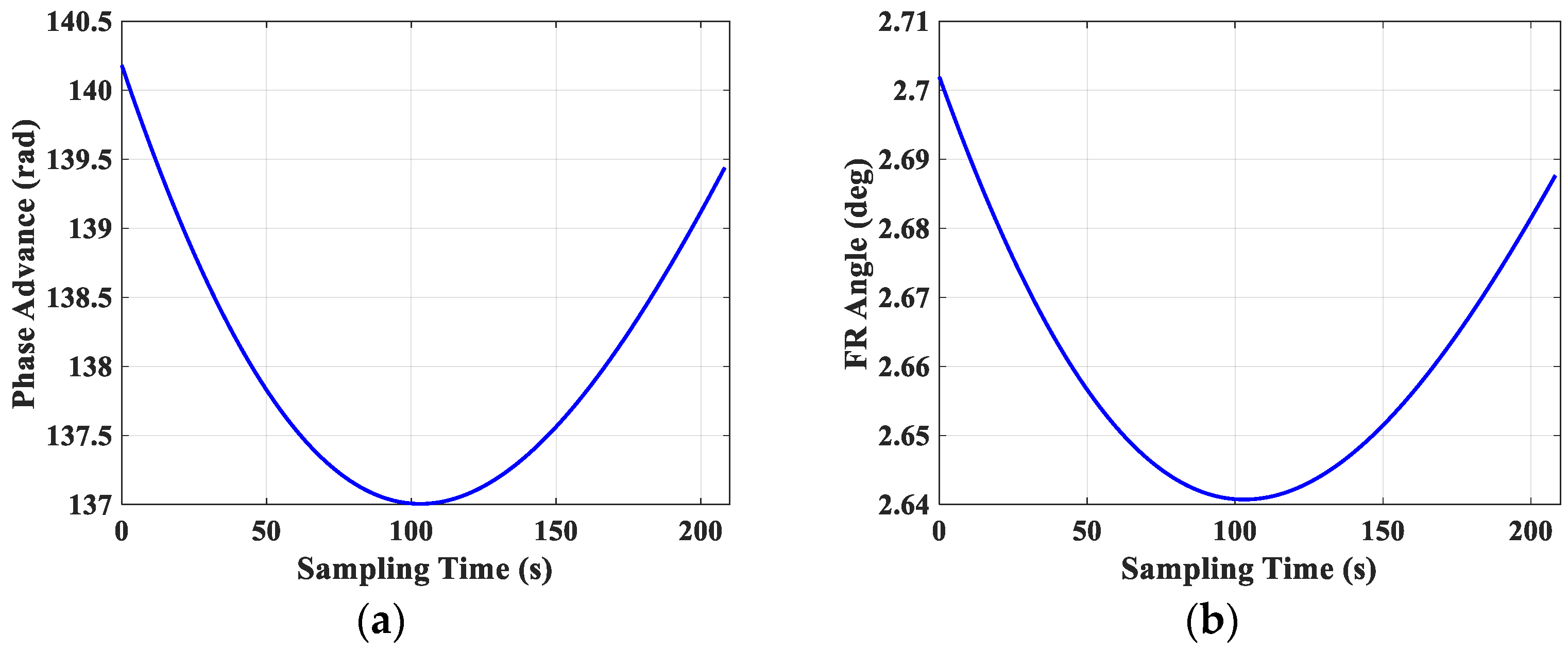
The measured TEC on 1 October 2015 (36°N, 84°W) from the United States Total Electron Content (USTEC) is adopted as the time-variant TEC (shown in Figure 5) [46]. During the simulation, only part of the TEC is used according to the integrated time, which is shown in Figure 5b corresponding to the area marked with the green box in Figure 5a. Firstly, the ionospheric effect error, including phase advance and FR angle, is calculated from the TEC in Figure 5b according to Equations (5) and (11), shown in Figure 6. Then, the ionospheric effect error is added during the echo simulation. In Figure 7, the affected FP SAR images are shown after imaging processing with the affected echoes.
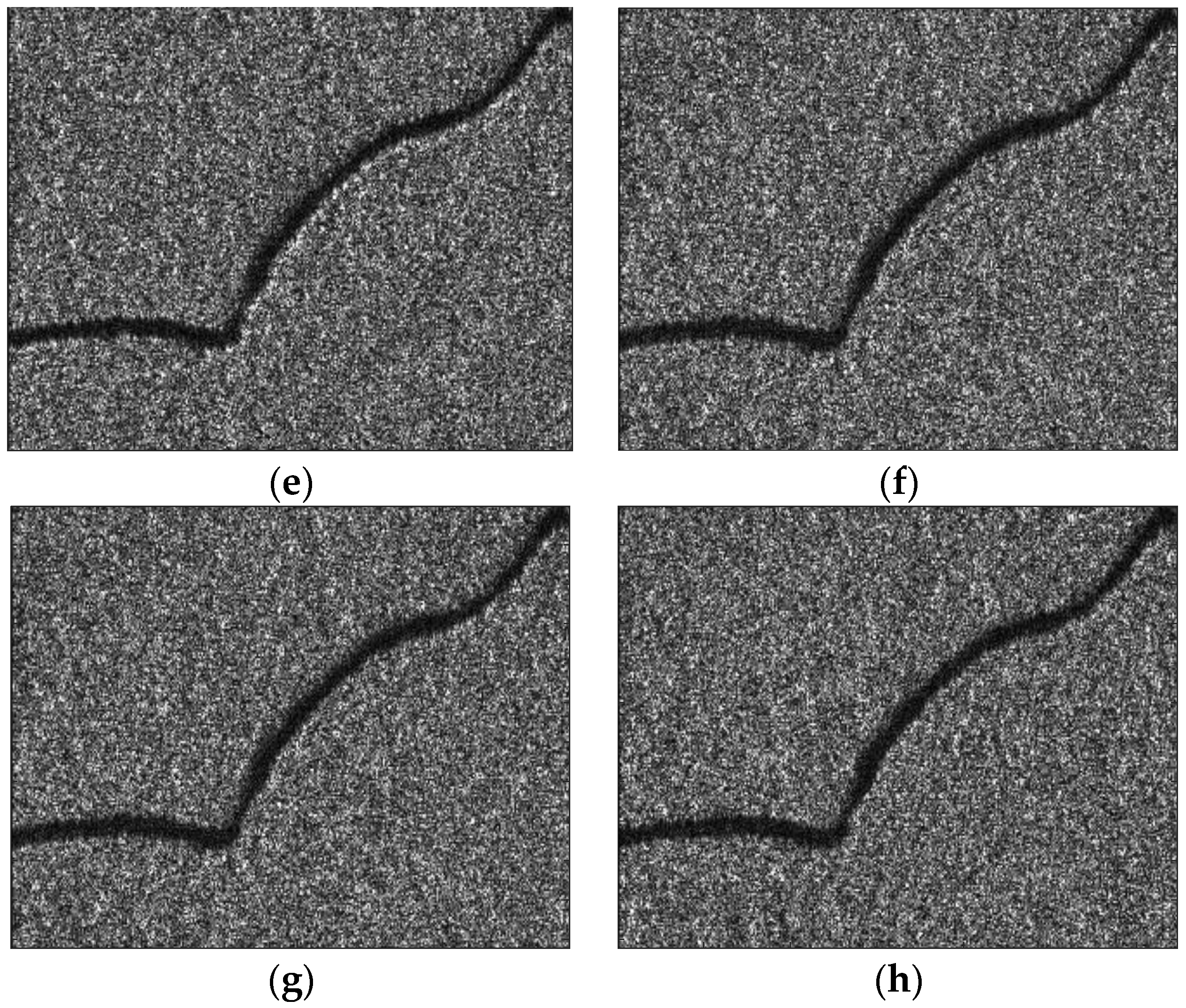
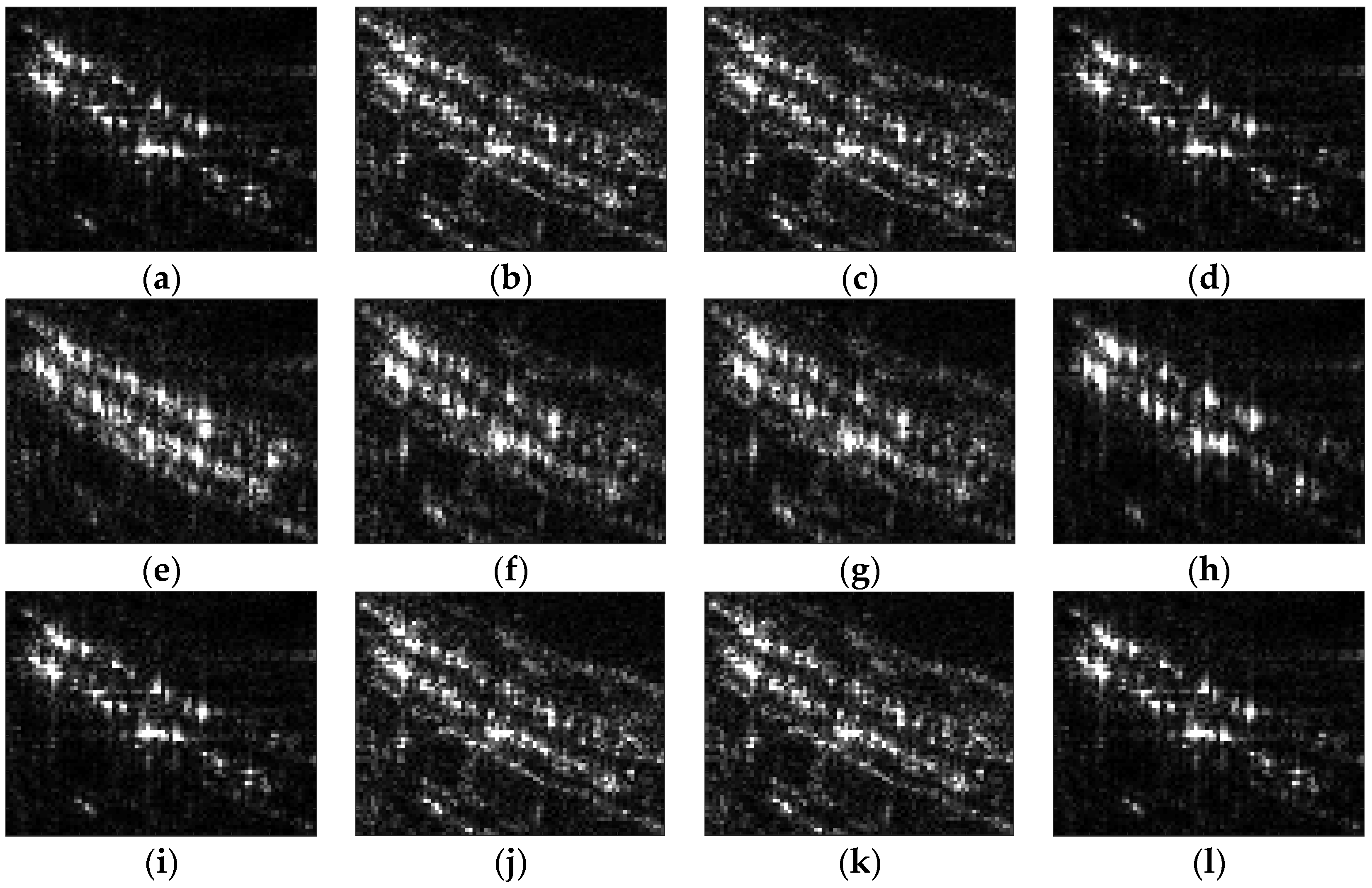
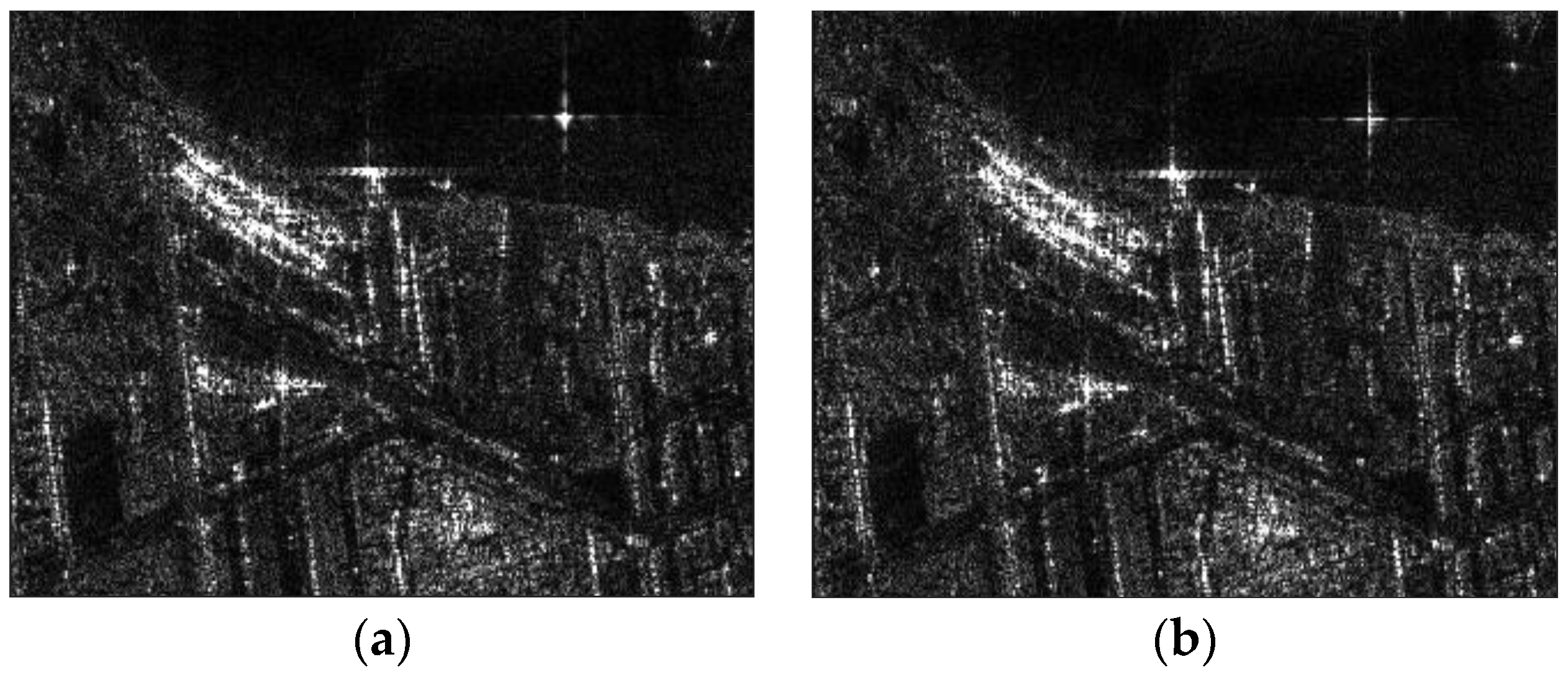
Comparing with the original images in Figure 4, the strong scattering points in Figure 7 become defocused in the azimuth direction, especially for the heterogeneous scene. The distortion in the range direction is not obvious, which confirms the QPE analysis in Section 2. The detailed comparison for the area marked with the red box in Figure 4 is shown in Figure 8, which reflects the time-variant ionospheric effect on the azimuth signal more distinctly. By contrast, the distortion of the homogenous scene is not that visually obvious, except for the blurring at the water–land boundary. In order to evaluate the impact from the ionosphere quantitatively, the correlation coefficient is introduced here. According to the statistical result in Table 2, the correlation coefficient of each channel declines nearly by half, and the cross-polarized channel degenerates particularly. The profile of the artificially placed point target (area marked with the yellow box in Figure 4) is also given in Figure 9. According to the evaluation of the imaging quality in Table 3, it is obvious that the azimuth signal gets defocused while the range signal is still good.
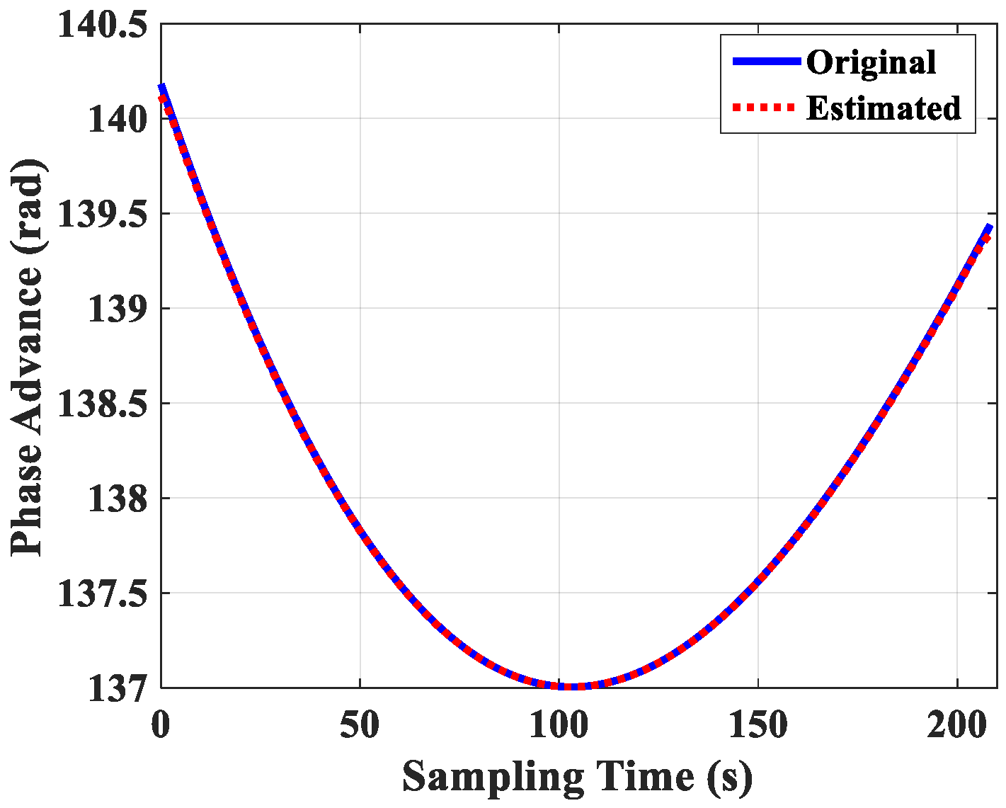
The compensation result with the proposed method is shown in Figure 8, Figure 9 and Figure 10, and the comparative result with PGA is also provided. During FR estimation, the size of the smoothing window along the azimuth direction is 64, and all the samplings of the range signal are used considering the uniformity of TEC in the range direction. The affected image is refocused after compensating with the proposed method for both scenes, while PGA is only valid for the heterogeneous scene, which conforms to its applicability with strong scattering points. The correlation coefficient and evaluation of imaging quality are also given in Table 2 and Table 3, respectively, proving the perfect performance of the proposed method and its good adaptability to different scenes. We also compare the original phase advance in the simulation and the estimated value during compensation (shown in Figure 11). The mean and standard deviation (STD) of error of the phase advance are 0.004 rad and 0.008 rad, respectively, which are quite small to guarantee the quality of imaging and polarization.
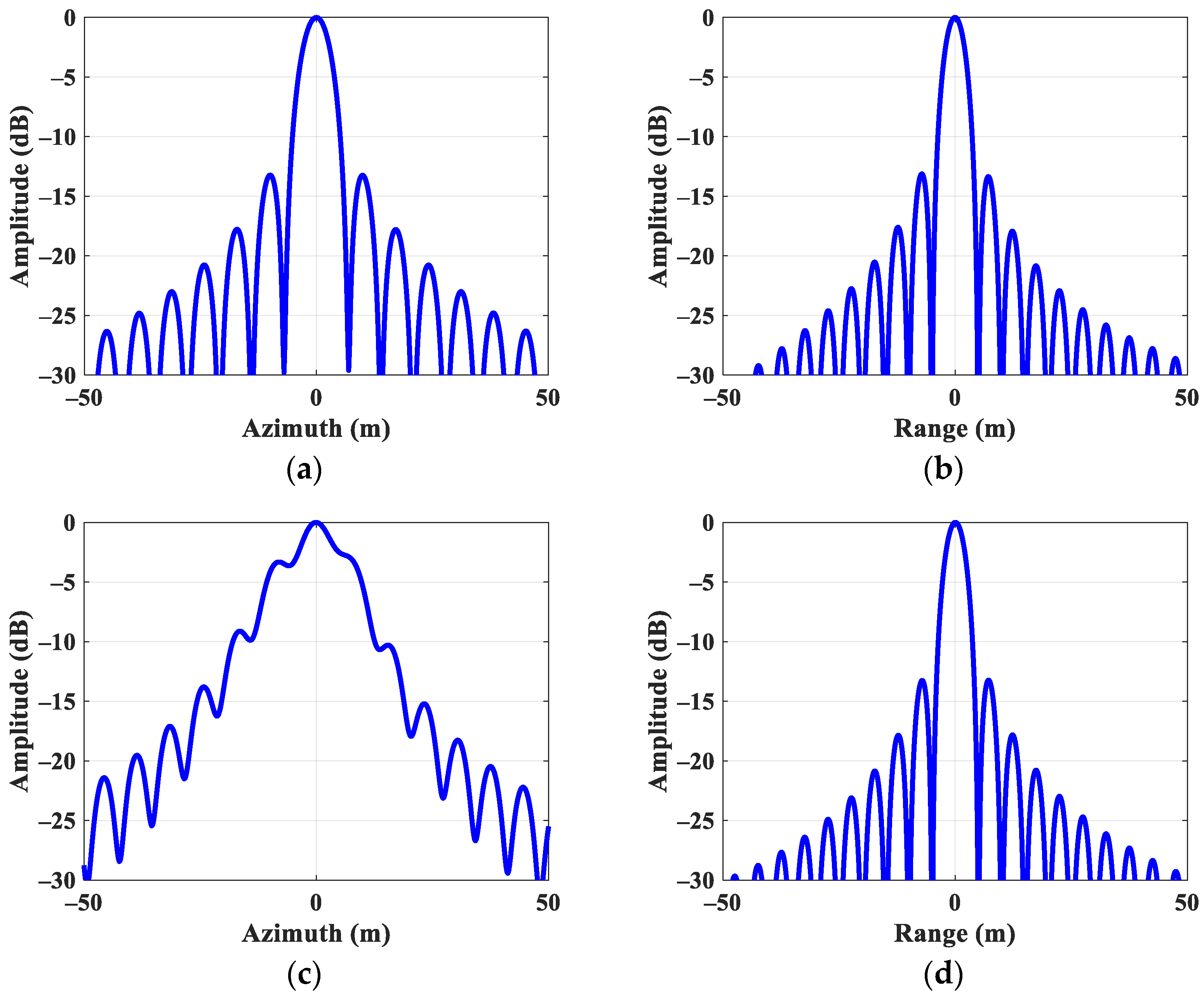
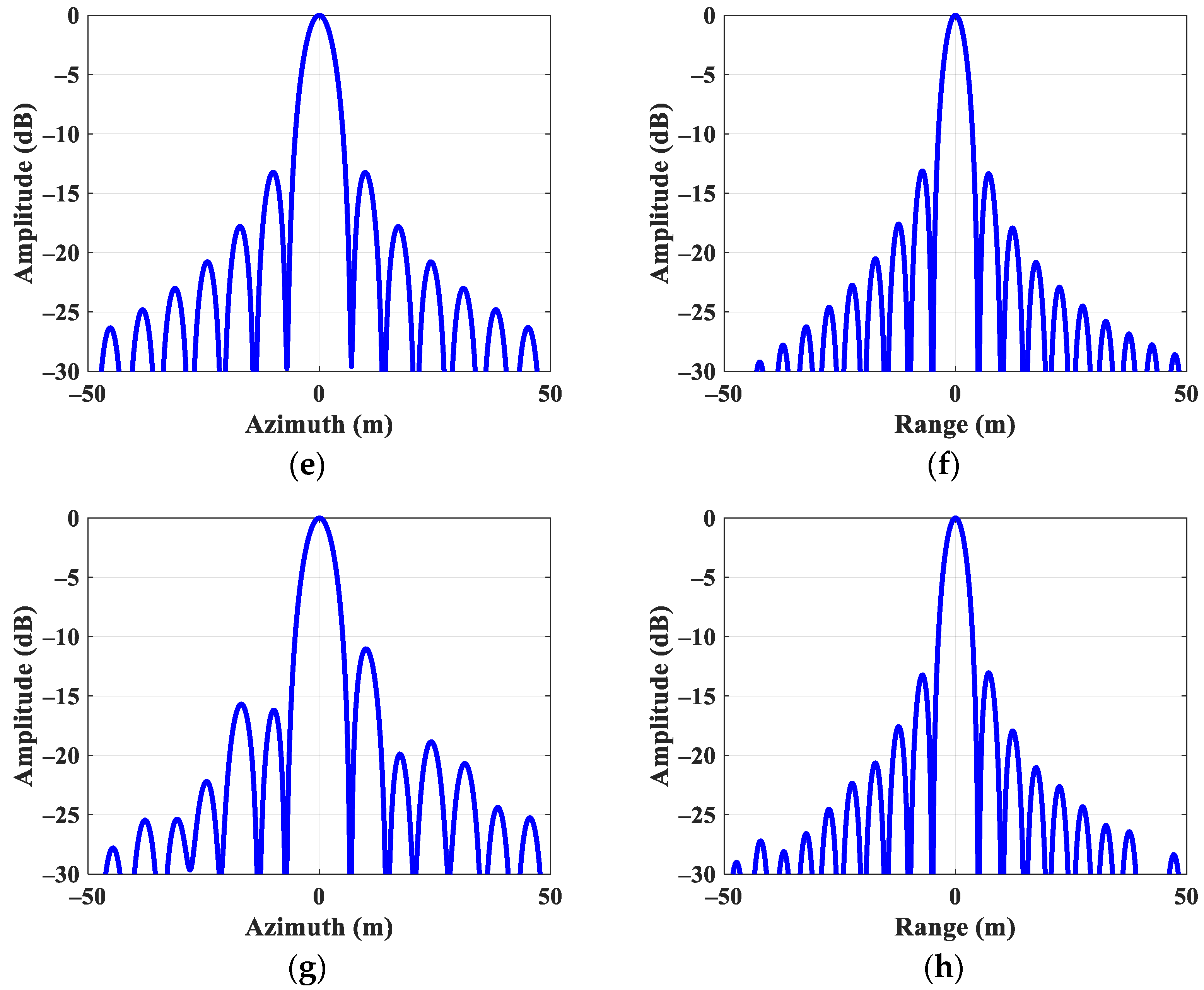
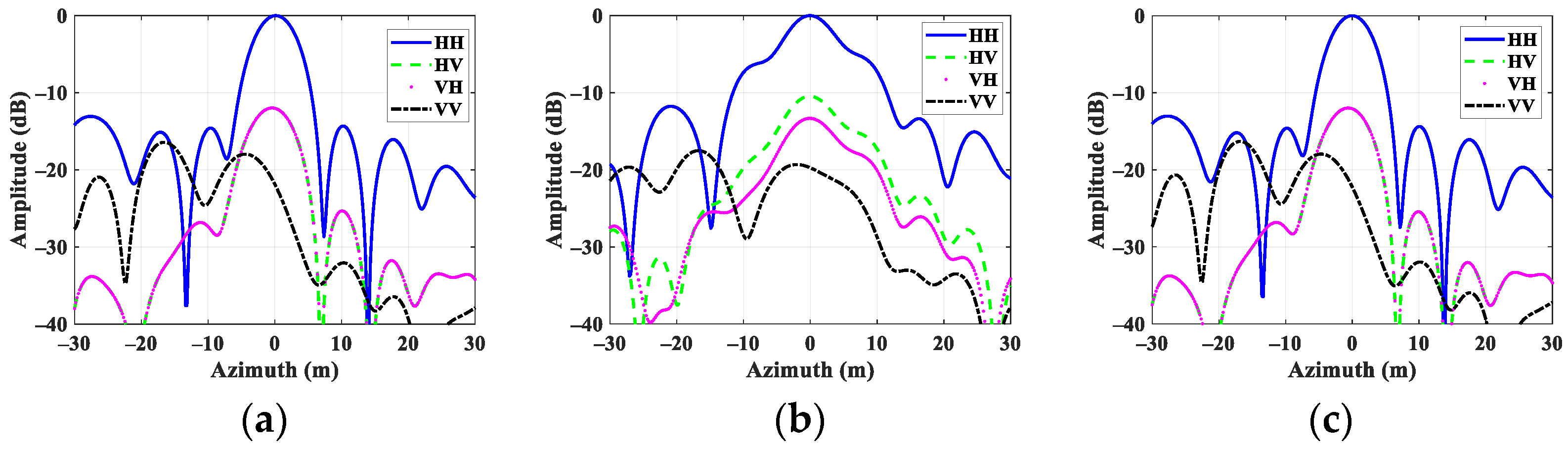
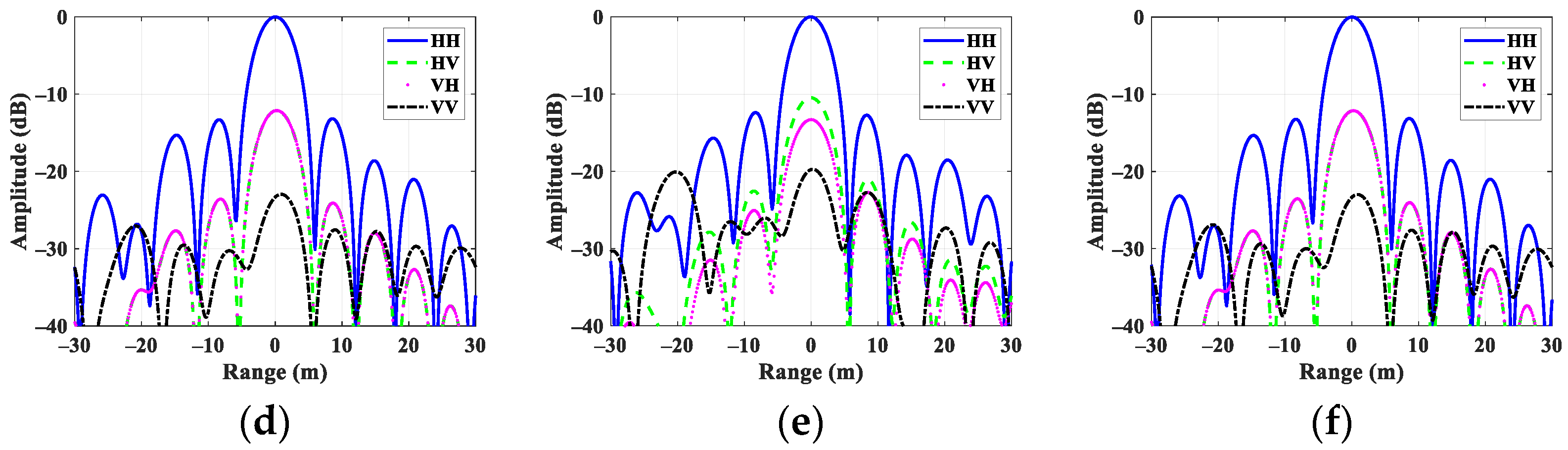
Moreover, in order to make the impact of the ionospheric effects and the performance of compensation for different polarimetric channels clearer, a strong scattering area within one sampling unit (area marked with the green box in Figure 4) is picked out to provide the profiles in both the azimuth and range directions in Figure 12. Comparing the azimuth and range profiles of the affected area in Figure 12b,e, it is obvious that the ionospheric effects on the azimuth signal is more severe than that of the range signal, which is consistent with the analyses and simulations above. In addition, the compensated profiles in Figure 12c,f also indicate the effectiveness of the proposed method, which could well solve the defocusing problems and recover the distributions of intensity for different polarimetric channels simultaneously.
4.2. Performance Analysis
The compensating performance of the proposed method is determined by the estimation of the ionospheric phase in (21). As the geomagnetic field can be obtained accurately based on the International Geomagnetic Reference Field (IGRF), the only factor determining the compensation is the accuracy of the FR angle. According to the polarimetric scattering model of the linearly FP SAR as shown below, two kinds of errors will lead to the misestimation of the FR angle: one is the polarimetric calibration error including the crosstalk and channel imbalance; the other is the thermal noise [47].
where δi, i = 1–4, represents the crosstalk, fi, i = 1–2, represents the channel imbalance, and Ni, i = 1–4, represents the thermal noise in each polarimetric channel.
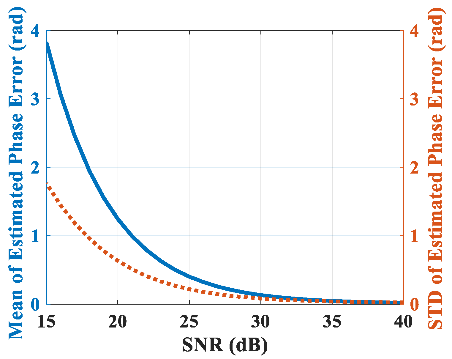
Based on the simulated FR SAR data in Section 4.1, the impact of the polarimetric calibration error and thermal noise is analyzed quantitatively. The simulation parameters are given in Table 4. Due to the error of the thermal noise and polarimetric calibration, the FR estimation becomes biased [47]. Thus, both the mean and STD of the estimation error are calculated to evaluate the performance. The mean of the phase error can be treated as a constant for each sampling time, which will not lead to the defocusing in azimuth. However, the corresponding constant TEC at each sampling time will deteriorate the range signal according to (9). The STD of the phase error, on the other hand, represents the randomness of the ionospheric phase within the integrated time, which will lead to the distortion in azimuth.
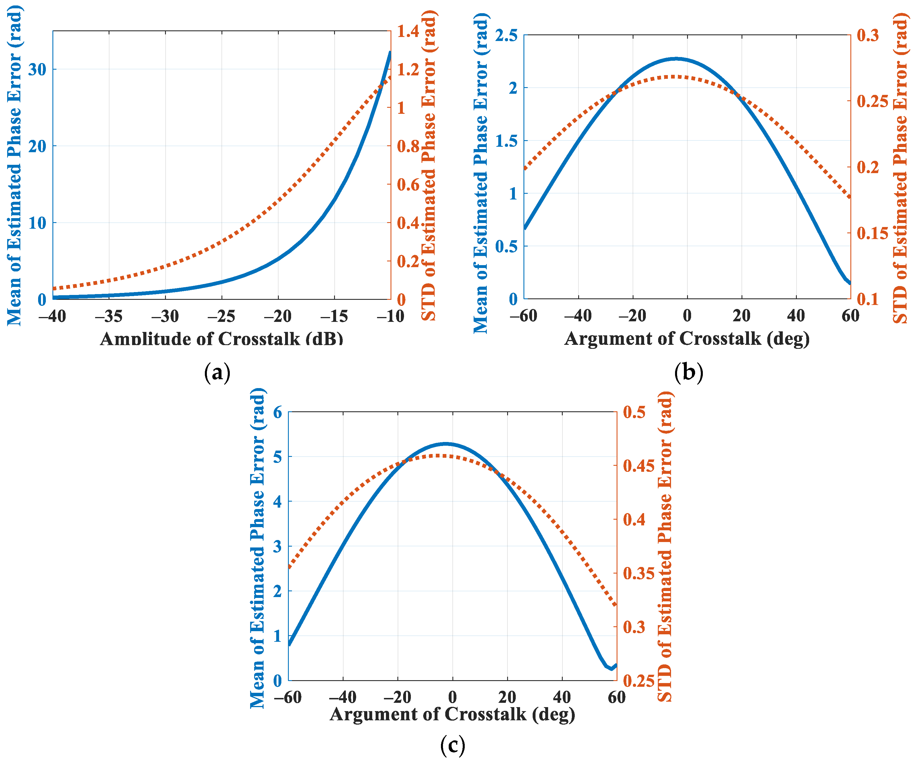
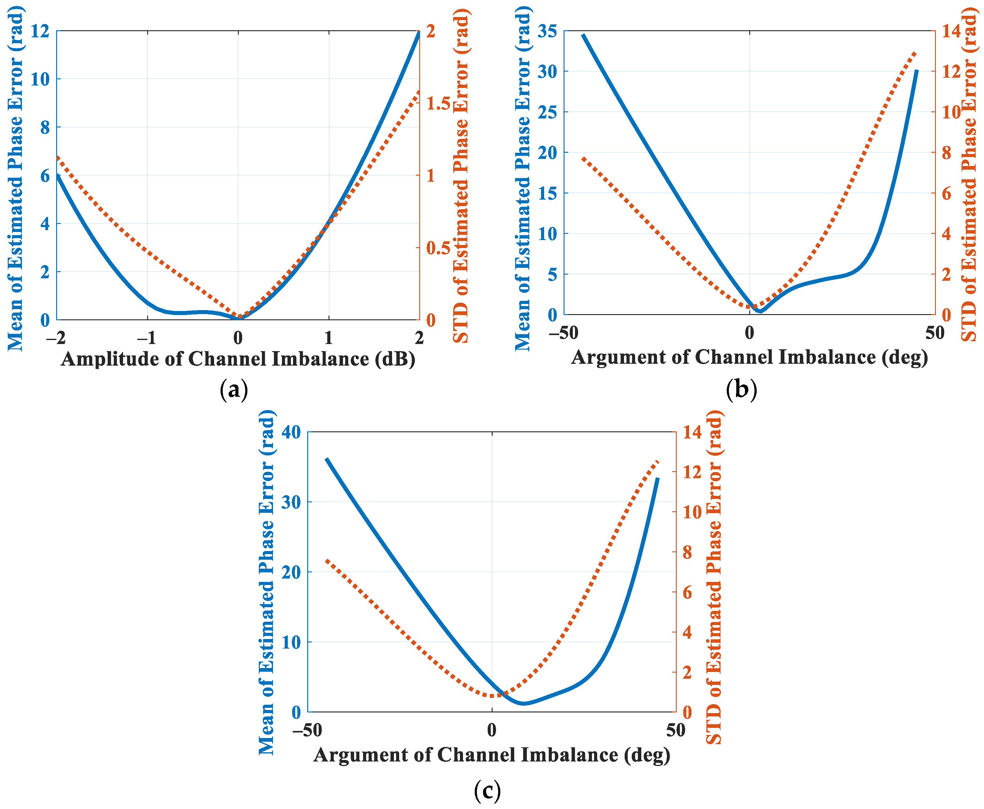
For the thermal noise, the error of the estimated phase is calculated in Figure 13, indicating that the error becomes large as the SNR decreases. If we take π/4 as the error threshold for imaging, the SNR should be better than 18.96 dB to guarantee the compensation accuracy for both the azimuth and range signals. For the amplitude of crosstalk, the mean of the estimated phase error is much more severe than that of STD (in Figure 14a), which means the interference from the quadrature channel will cause a larger overall bias than a fluctuation. In comparison, the argument of crosstalk is secondarily determining, or even the partial introduction of argument is conducive to the elimination of interference. Similarly, an error threshold of −15.63 dB for crosstalk is drawn according to the simulation result. By contrast, the influence from the channel imbalance is a little different. According to the result in Figure 15, if the channel imbalance can be kept within −1.02 dB to 0.31 dB, the residual error after ionospheric compensation will not affect imaging. Meanwhile, for the argument part, the restriction is more severe. According to the results in Figure 15b,c, the trend of error caused by the channel imbalance remains almost unchanged with different amplitudes of channel imbalance. It means the argument matters more than that of the amplitude for channel imbalance. Thus, the argument of channel imbalance is suggested to be maintained at zero as far as possible so as to guarantee the compensation accuracy.
5. Discussion
According to the simulation in Section 4.1, the performance of the PGA and the proposed method is contrasting, especially for the homogenous scene. As for the PGA itself, the estimated error within the synthetic aperture should be the same for each scattering point, which is quite a strict assumption. In order to meet this condition, the shifting and windowing are necessary to acquire the echo of the isolated scattering point approximatively. However, the interference from the background clutter and adjacent scatters cannot be completely eliminated in real SAR images. Thus, the PGA will predictably lose its efficiency for the homogenous image (such as the rainforest and desert) and the heterogeneous image with low SCR/SNR. Moreover, the PGA processing does not depend on the analytic error model and removes the error directly from the image to increase the visual effect. Thus, the true error at each sampling, i.e., the time-variant ionospheric error in the echo instead of the image, could not be obtained. This is why the estimated phase advance of the proposed method is shown in Figure 11, while the PGA cannot be shown.
The proposed method uses the FR angle to estimate the time-variant TEC, which is born with two-dimensional resolution capability corresponding to the SAR data. Thus, the time-variant characteristic of TEC can be accurately reflected based on the pulse sampling. Moreover, the Bickel and Bates’s FR estimation is based on the argument of the circular basis, which has less restriction on the target. Moreover, the variance of the estimated FR is only related with the SNR level according to the theoretical error model [48]. Thus, the performance of applicability with different scenes for the proposed method is quite good, as we have shown in Section 4. As for the polarimetric calibration error, the amplitude and phase of the distortions could give rise to a noticeable bias in the FR estimation, which will affect the ionospheric phase correction. The amplitude of crosstalk and the argument of channel imbalance are proved to have a greater impact on the FR bias, which is consistent with Quegan’s analysis in [47]. Thus, the polarimetric calibration of the FP SAR system is quite necessary, which could greatly weaken the impact from polarimetric distortions.
Of course, there are still some problems that need to be further considered for the proposed method:
- (1)
- The first problem concerns about the “zero Faraday rotation area”. According to the FR model in (11), the FR is closely related to the angle between the beam and geomagnetic field. If the angle is close to 90°, the FR angle will be almost zero. Combining the distribution of the geomagnetic field and the typical side-looking model of SAR, the zero FR area usually appears near the equator [39]. In this particular area, the TEC cannot be accurately estimated with the FR angle, so the corresponding method becomes invalid. Aiming to solve this problem, we are now trying to use the spatial variation of the geomagnetic field under a multi-dimensional model of the ionosphere to avoid the zero FR area problem.
- (2)
- The other problem concerns the limitation of the observing swath with FP mode. Due to the double of PRF, the observing swath is reduced by half compared to the single-polarimetric mode. Thus, for the wide swath modes, such as ScanSAR and TOPSAR, the FP observation is traditionally abandoned. The GEO-SAR system is proposed and recommended owing to its almost global coverage capability. Thus, the FP data may not be provided for ionospheric effect compensation. To solve this contradiction, we are working on the transmission of orthogonal polarimetric signals with frequency division multiplexing (FDM) technology, which can extend the swath and well preserve the FP information.
6. Conclusions
In this paper, a compensation method of background ionospheric effects on L-band GEO-SAR with fully polarimetric data is proposed. Based on the Faraday rotation estimation, the time-variant TEC can be acquired accurately for ionospheric effect compensation.
Considering the ultra-long synthetic aperture time of the GEO-SAR system, the time-variant characteristic of the background ionosphere is mainly concerned, and the corresponding error model is established. Combining the coherent integration of the SAR signal, decompression processing is firstly used to reconstruct the echo for each polarimetric channel. Then, the time-variant TEC is obtained accurately based on FR angle estimation. Finally, the ionospheric effect is compensated for according to the error model we established previously.
With the real FP SAR data from ALOS-2 and the measured time-variant TEC from USTEC, the simulation is conducted to prove the effectiveness and performance of the proposed compensation method. For different scenes, the proposed method could recover the data to more than 90% of the correlation coefficient, and the residual error of phase is less than 0.01 rad. Two kinds of typical error sources are also discussed to evaluate the performance of the method, including the thermal noise and the polarimetric calibration errors, from which the thresholds of error are given to guarantee compensation accuracy, in particular 18.96 dB for SNR, −15.63 dB for crosstalk and −1.02 dB to 0.31 dB for the amplitude of the channel imbalance, and the argument of the channel imbalance is suggested to be maintained as to zero as possible. Furthermore, the comparison between the proposed and existing methods is discussed in detail and the preliminary work of our follow-up research is also presented.
Author Contributions
Conceptualization and methodology, W.G.; software and formal analysis, W.G.; validation, P.X.; writing—original draft preparation, W.G.; writing—review and editing, P.X. and X.G. All authors have read and agreed to the published version of the manuscript.
Funding
This research was supported by the Fundamental Research Funds for the Central Universities under grant number ZYTS23107.
Data Availability Statement
The measured TEC data from the United States Total Electron Content (USTEC) is available from the National Oceanic and Atmospheric Administration (NOAA) at https://www.swpc.noaa.gov/products/us-total-electron-content (accessed on 1 October 2015). The fully polarimetric SAR data from ALOS-2 are not publicly available due to privacy restrictions.
Conflicts of Interest
The authors declare no conflict of interest.
References
- Rosenqvist, A.; Shimada, M.; Ito, N.; Watanabe, M. ALOS PALSAR: A Pathfinder Mission for Global-Scale Monitoring of the Environment. IEEE Trans. Geosci. Remote Sens. 2007, 45, 3307–3316. [Google Scholar] [CrossRef]
- Shimada, M. ALOS-2 Science Program. In Proceedings of the IEEE International Geoscience and Remote Sensing Symposium 2013, Melbourne, VIC, Australia, 21–26 July 2013; pp. 2400–2403. [Google Scholar]
- Motohka, T.; Kankaku, Y.; Miura, S.; Suzuki, S. ALOS-4 L-Band SAR Observation Concept and Development Status. In Proceedings of the IEEE International Geoscience and Remote Sensing Symposium 2020, Waikoloa, HI, USA, 26 September–2 October 2013; pp. 3792–3794. [Google Scholar]
- Guarnieri, M.A.; Djalaili, F.; Schulz, D.; Khang, V.T.; Recchia, A.; Rocca, F.; Giudici, D.; Hobbs, S.; Strozzi, T.; Werner, C.; et al. Wide Coverage, Fine Resolution, Geosynchronous SAR for Atmosphere and Terrain Observations. In Proceedings of the ESA Living Planet Symposium 2013, Edinburgh, UK, 9–13 September 2013; p. 147. [Google Scholar]
- Wadge, G.; Guarnieri, M.A.; Hobbs, S.E.; Schulz, D. Potential Atmospheric and Terrestrial Applications of a Geosynchronous Radar. In Proceedings of the IEEE Geoscience and Remote Sensing Symposium 2014, Quebec City, QC, Canada, 13–18 July 2014; pp. 946–949. [Google Scholar]
- Hobbs, S.; Guarnieri, A.M.; Wadge, G.; Schulz, D. GeoSTARe Initial Mission Design. In Proceedings of the IEEE International Geoscience and Remote Sensing Symposium 2014, Quebec City, QC, Canada, 13–18 July 2014; pp. 92–95. [Google Scholar]
- Ruiz-Rodon, J.; Broquetas, A.; Makhoul, E.; Guarnieri, A.M.; Rocca, F. Nearly Zero Inclination Geosynchronous SAR Mission Analysis With Long Integration Time for Earth Observation. IEEE Trans. Geosci. Remote Sens. 2014, 45, 6379–6391. [Google Scholar] [CrossRef]
- Guarnieri, A.M.; Perletta, L.; Rocca, F.; Scapin, D.; Tebaldini, S.; Broquetas, A.; Ruiz-Rodon, J. Design of a Geosynchronous SAR System for Water-vapour Maps and Deformation Estimation. In Proceedings of the ESA Fringe Workshop 2011, Frascati, Italy, 19–23 September 2011; pp. 1–5. [Google Scholar]
- Hobbs, S.; Sanchez, J.P. Laplace Plane and Low Inclination Geosynchronous Radar Mission Design. Sci. China Inf. Sci. 2017, 60, 060305:1–060305:10. [Google Scholar] [CrossRef]
- Hu, C.; Li, Y.; Dong, X.; Wang, R.; Ao, D. Performance Analysis of L-Band Geosynchronous SAR Imaging in the Presence of Ionospheric Scintillation. IEEE Trans. Geosci. Remote Sens. 2017, 55, 159–172. [Google Scholar] [CrossRef]
- Xu, Z.; Wu, J.; Wu, Z. A Survey of Ionospheric Effects on Space-based Radar. Waves Random Media 2004, 14, S199–S273. [Google Scholar] [CrossRef]
- Carrano, C.S.; Groves, K.M.; Caton, R.G. Simulating the Impacts of Ionospheric Scintillation on L band SAR Image Formation. Radio Sci. 2012, 47, 1–14. [Google Scholar] [CrossRef]
- European Space Agency (ESA). BIOMASS Report for Mission Selection an Earth Explorer to Observe Forest Biomass. Available online: https://earth.esa.int/eogateway/documents/20142/37627/BIOMASS-Report-for-Mission-Selection-An-Earth-Explorer-to-observe-forest-biomass.pdf (accessed on 30 May 2012).
- Armand, N.A.; Smirnov, V.M.; Hagfors, T. Distortion of Radar Pulses by the Martian Ionosphere. Radio Sci. 2003, 38, 11-1–11-12. [Google Scholar] [CrossRef]
- Belcher, D.P. Theoretical Limits on SAR Imposed by the Ionosphere. IET Radar Sonar Navig. 2008, 2, 435–448. [Google Scholar] [CrossRef]
- Hu, C.; Tian, Y.; Yang, X.; Zeng, T.; Long, T.; Dong, X. Background Ionosphere Effects on Geosynchronous SAR Focusing: Theoretical Analysis and Verification Based on the BeiDou Navigation Satellite System (BDS). IEEE J. Sel. Top. Appl. Earth Obs. Remote Sens. 2016, 9, 1143–1162. [Google Scholar] [CrossRef]
- Tian, Y.; Hu, C.; Dong, X.; Zeng, T.; Long, T.; Lin, K.; Zhang, X. Theoretical Analysis and Verification of Time Variation of Background Ionosphere on Geosynchronous SAR Imaging. IEEE Geosci. Remote Sens. Lett. 2015, 12, 721–725. [Google Scholar] [CrossRef]
- Li, Z.; Chen, J. Simultaneous Measurement of Time-variant TEC for Compensating Ionospheric Effect on Geosynchronous SAR using HF-radar. In Proceedings of the IEEE 13th International Conference on Signal Processing 2016, Chengdu, China, 6–10 November 2016; pp. 87–90. [Google Scholar]
- Bruno, D.; Hobbs, S. Radar Imaging From Geosynchronous Orbit: Temporal Decorrelation Aspects. IEEE Trans. Geosci. Remote Sens. 2010, 48, 2924–2929. [Google Scholar] [CrossRef]
- Long, T.; Hu, C.; Ding, Z.; Dong, X.; Tian, W.; Zeng, T. Geosynchronous SAR: System and Signal Processing; Springer: Singapore, 2018. [Google Scholar]
- Li, Z.; Quegan, S.; Chen, J.; Rogers, N.C. Performance Analysis of Phase Gradient Autofocus for Compensating Ionospheric Phase Scintillation in BIOMASS P-Band SAR Data. IEEE Geosci. Remote Sens. Lett. 2015, 12, 1367–1371. [Google Scholar]
- Dong, X.; Hu, C.; Tian, Y.; Tian, W.; Li, Y.; Long, T. Experimental Study of Ionospheric Impacts on Geosynchronous SAR Using GPS Signals. IEEE J. Sel. Top. Appl. Earth Obs. Remote Sens. 2016, 9, 2171–2183. [Google Scholar] [CrossRef]
- Guarnieri, A.M.; Leanza, A.; Recchia, A.; Tebaldini, S.; Venuti, G. Atmospheric Phase Screen in GEO-SAR: Estimation and Compensation. IEEE Trans. Geosci. Remote Sens. 2017, 56, 1668–1679. [Google Scholar] [CrossRef]
- Liang, X.; Li, Z. Analysis and Compensation of Ionospheric Time-Variant TEC Effect on GEO SAR Focusing. Prog. Electromagn. Res. M. 2019, 77, 205–213. [Google Scholar] [CrossRef] [Green Version]
- Wang, R.; Hu, C.; Li, Y.; Hobbs, S.E.; Tian, W.; Dong, X.; Chen, L. Joint Amplitude-Phase Compensation for Ionospheric Scintillation in GEO SAR Imaging. IEEE Trans. Geosci. Remote Sens. 2017, 55, 3454–3465. [Google Scholar] [CrossRef]
- Ding, Z.; Zhu, K.; Zhang, T.; Li, L.; Wang, Y.; Wang, G.; Gao, Y.; Wei, Y.; Zeng, T. An Autofocus Back Projection Algorithm for GEO SAR Based on Minimum Entropy. IEEE Trans. Geosci. Remote Sens. 2022, 60, 5226114. [Google Scholar] [CrossRef]
- Zhang, X.; Huang, P.; Wang, W. New Method to Correct Background Ionospheric Phase Distortion in GEO SAR. In Proceedings of the IET International Radar Conference 2015, Hangzhou, China, 14–16 October 2015; pp. 1–4. [Google Scholar]
- Meyer, F.; Bamler, R.; Jakowski, N.; Fritz, T. The Potential of Low-Frequency SAR Systems for Mapping Ionospheric TEC Distributions. IEEE Geosci. Remote Sens. Lett. 2006, 3, 560–564. [Google Scholar] [CrossRef]
- Jehle, M.; Frey, O.; Small, D.; Meier, E. Measurement of Ionospheric TEC in Spaceborne SAR Data. IEEE Trans. Geosci. Remote Sens. 2010, 6, 2460–2468. [Google Scholar] [CrossRef]
- Carrara, W.G.; Goodman, R.S.; Majewski, R.M. Spotlight Synthetic Aperture Radar Signal Processing Algorithms; Artech House: Boston, MA, USA; London, UK, 1995. [Google Scholar]
- Liu, L.; Chen, Y. Statistical Analysis of Solar Activity Variations of Total Electron Content Derived at Jet Propulsion Laboratory from GPS Observations. J. Geophys. Res. 2009, 114, A10311. [Google Scholar] [CrossRef] [Green Version]
- Dach, R.; Schaer, S.; Arnold, D.; Kalarus, M.S.; Prange, L.; Stebler, P.; Jäggi, A.; Villiger, A. CODE Final Product Series for the IGS. Available online: https://boris.unibe.ch/id/eprint/143807 (accessed on 4 May 2020).
- Lin, H.; Deng, Y.; Zhang, H.; Wang, J.; Liang, D.; Fang, T.; Wang, R. Estimating and Removing Ionospheric Effects for L-Band Spaceborne Bistatic SAR. IEEE Trans. Geosci. Remote Sens. 2022, 60, 5219816. [Google Scholar] [CrossRef]
- Lawrence, R.S.; Little, C.G.; Chivers, H.J.A. A Survey of Ionospheric Effects upon Earth-space Radio Propagation. Proc. IEEE 1964, 52, 4–27. [Google Scholar] [CrossRef]
- Wright, P.A.; Quegan, S.; Wheadon, N.S.; Hall, C.D. Faraday Rotation Effects on L-band Spaceborne SAR Data. IEEE Trans. Geosci. Remote Sens. 2003, 41, 2735–2744. [Google Scholar] [CrossRef]
- Bickel, S.H.; Bates, R.H.T. Effects of Magneto-ionic Propagation on the Polarization Scattering Matrix. Proc. IEEE 1965, 53, 1089–1091. [Google Scholar] [CrossRef]
- Freeman, A. Calibration of Linearly Polarized Polarimetric SAR Data Subject to Faraday Rotation. IEEE Trans. Geosci. Remote Sens. 2004, 42, 1617–1624. [Google Scholar] [CrossRef]
- Chen, J.; Quegan, S. Improved Estimators of Faraday Rotation in Spaceborne Polarimetric SAR Data. IEEE Geosci. Remote Sens. Lett. 2010, 7, 846–850. [Google Scholar] [CrossRef]
- Kim, J.S.; Papathanassiou, K.P.; Scheiber, R.; Quegan, S. Correcting Distortion of Polarimetric SAR Data Induced by Ionospheric Scintillation. IEEE Trans. Geosci. Remote Sens. 2015, 53, 6319–6335. [Google Scholar]
- Kim, J.S.; Papathanassiou, K.P.; Quegan, S.; Rogers, N. Estimation and Correction of Scintillation Effects on Spaceborne P-band SAR Images. In Proceedings of the IEEE International Geoscience and Remote Sensing Symposium 2012, Munich, Germany, 22–27 July 2012; pp. 5101–5104. [Google Scholar]
- Hu, C.; Tian, Y.; Zeng, T.; Long, T.; Dong, X. Adaptive Secondary Range Compression Algorithm in Geosynchronous SAR. IEEE J. Sel. Top. Appl. Earth Obs. Remote Sens. 2016, 9, 1397–1413. [Google Scholar] [CrossRef]
- Hu, C.; Long, T.; Liu, Z.; Zeng, T.; Tian, Y. An Improved Frequency Domain Focusing Method in Geosynchronous SAR. IEEE Trans. Geosci. Remote Sens. 2014, 52, 5514–5528. [Google Scholar]
- Li, D.; Wu, M.; Sun, Z.; He, F.; Dong, Z. Modeling and Processing of Two-Dimensional Spatial-Variant Geosynchronous SAR Data. IEEE J. Sel. Top. Appl. Earth Obs. Remote Sens. 2015, 8, 3999–4009. [Google Scholar] [CrossRef]
- Li, D.; Rodriguez-Cassola, M.; Prats-Iraola, P.; Wu, M.; Moreira, M. Reverse Backprojection Algorithm for the Accurate Generation of SAR Raw Data of Natural Scenes. IEEE Geosci. Remote Sens. Lett. 2017, 14, 2072–2076. [Google Scholar] [CrossRef]
- Yu, Z.; Lin, P.; Xiao, P.; Kang, L.; Li, C. Correcting Spatial Variance of RCM for GEO SAR Imaging Based on Time-Frequency Scaling. Sensors 2016, 16, 1091. [Google Scholar] [CrossRef] [PubMed] [Green Version]
- National Oceanic and Atmospheric Administration (NOAA). U.S. Total Electron Content. Available online: https://www.swpc.noaa.gov/products/us-total-electron-content (accessed on 1 October 2015).
- Quegan, S.; Lomas, M.R. The Impact of System Effects on Estimates of Faraday Rotation from Synthetic Aperture Radar Measurements. IEEE Trans. Geosci. Remote Sens. 2015, 53, 4284–4298. [Google Scholar] [CrossRef]
- Rodriguez, E.; Martin, J.M. Theory and Design of Interferometric Synthetic Aperture Radars. IEE Proc. F-Radar Signal Process. 1992, 139, 147–159. [Google Scholar] [CrossRef]
Figure 1.
The time–frequency relationship of the chirp signal under ionospheric effects. The red arrow line represents the group delay of the chirp signal.
Figure 1.
The time–frequency relationship of the chirp signal under ionospheric effects. The red arrow line represents the group delay of the chirp signal.

Figure 2.
The diagram of time-variant background ionospheric effects on radar pluses with TEC(t) at each pulse sampling time within the synthetic aperture.
Figure 2.
The diagram of time-variant background ionospheric effects on radar pluses with TEC(t) at each pulse sampling time within the synthetic aperture.

Figure 3.
The compensating flow diagram of the proposed method.

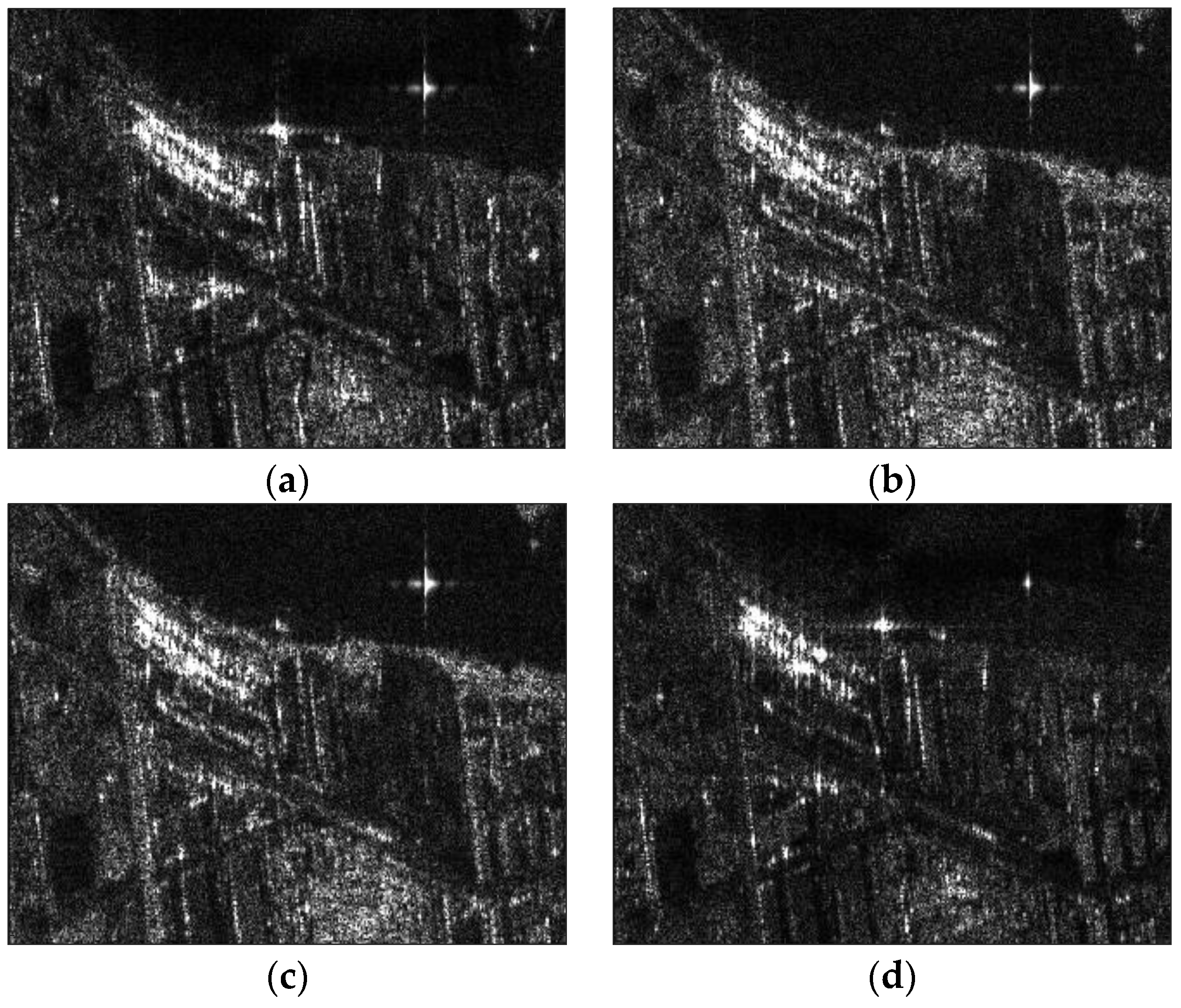
Figure 4.
The original FP SAR images. (a–d) HH, HV, VH and VV images with artificial targets for the heterogeneous scene; (e–h) HH, HV, VH and VV images with rainforest for the homogeneous scene.
Figure 4.
The original FP SAR images. (a–d) HH, HV, VH and VV images with artificial targets for the heterogeneous scene; (e–h) HH, HV, VH and VV images with rainforest for the homogeneous scene.


Figure 5.
(a) The measured time-variant TEC from USTEC; (b) the part of the measured TEC used in the simulation (marked with the green box in (a)).
Figure 5.
(a) The measured time-variant TEC from USTEC; (b) the part of the measured TEC used in the simulation (marked with the green box in (a)).

Figure 6.
The ionospheric effect error used in the simulation. (a) The phase advance at the carrier frequency; (b) the FR angle.
Figure 6.
The ionospheric effect error used in the simulation. (a) The phase advance at the carrier frequency; (b) the FR angle.

Figure 7.
The affected FP SAR images. (a–d) HH, HV, VH and VV images with artificial targets for the heterogeneous scene; (e–h) HH, HV, VH and VV images with rainforest for the homogeneous scene.
Figure 7.
The affected FP SAR images. (a–d) HH, HV, VH and VV images with artificial targets for the heterogeneous scene; (e–h) HH, HV, VH and VV images with rainforest for the homogeneous scene.


Figure 8.
The comparison of the detailed FP SAR images with and without ionospheric effect and the compensated images. (a–d) detailed HH, HV, VH and VV images without ionospheric effect; (e–h) detailed HH, HV, VH and VV images with ionospheric effect; (i–l) detailed HH, HV, VH and VV compensated images.

Figure 9.
The azimuth and range profiles of the artificially placed point target. (a,b) The azimuth and range profiles of the original point target; (c,d) the azimuth and range profiles of the affected point target; (e,f) the azimuth and range profiles of the compensated point target with the proposed method; (g,h) the azimuth and range profiles of the compensated point target with the PGA.


Figure 10.
The compensated HH images with the proposed and PGA methods. (a) The compensated HH image with the proposed method for the heterogeneous scene; (b) the compensated HH image with the PGA for the heterogeneous scene; (c) the compensated HH image with the proposed method for the homogeneous scene; (d) the compensated HH image with the PGA for the homogeneous scene.


Figure 11.
The original phase advance in simulation and estimated value during compensation with the proposed method. The error of phase estimation is 0.004 rad for mean and 0.008 rad for standard deviation.
Figure 11.
The original phase advance in simulation and estimated value during compensation with the proposed method. The error of phase estimation is 0.004 rad for mean and 0.008 rad for standard deviation.

Figure 12.
The azimuth and range profiles of the strong scattering area for different polarimetric channels. (a–c) The azimuth profiles of the original, affected and compensated areas; (d–f) the range profiles of the original, affected and compensated areas.
Figure 12.
The azimuth and range profiles of the strong scattering area for different polarimetric channels. (a–c) The azimuth profiles of the original, affected and compensated areas; (d–f) the range profiles of the original, affected and compensated areas.


Figure 13.
The mean and STD of the estimated phase error changing with the SNR of imaging.

Figure 14.
The mean and STD of the estimated phase error changing with the crosstalk. (a) The estimated phase error changing with the amplitude of crosstalk; (b) the estimated phase error changing with the argument of crosstalk at −25 dB of amplitude; (c) the estimated phase error changing with the argument of crosstalk at −20 dB of amplitude.

Figure 15.
The mean and STD of the estimated phase error changing with the channel imbalance. (a) The estimated phase error changing with the amplitude of channel imbalance; (b) the estimated phase error changing with the argument of channel imbalance at 0.5 dB of amplitude; (c) the estimated phase error changing with the argument of channel imbalance at 1 dB of amplitude.


Table 1.
The simulation parameters.
| Parameter | Value |
|---|---|
| Orbit altitude | 35,793.29 km |
| Orbit inclination | 60 deg |
| Right ascension of ascending node | 97 deg |
| Wavelength | 0.24 m |
| Bandwidth | 30 MHz |
| Sampling rate | 33 MHz |
| Pulse repetition frequency | 75 Hz |
| Pulse width | 20 μs |
| Integrated time | 208 s |
Table 2.
The correlation coefficient between the original and the affected as well as the compensated FP SAR images (with the proposed method) for heterogeneous and homogeneous scenes.
Table 2.
The correlation coefficient between the original and the affected as well as the compensated FP SAR images (with the proposed method) for heterogeneous and homogeneous scenes.
| Channel | HH | HV | VH | VV | |
|---|---|---|---|---|---|
| Scene Type | |||||
| Heterogeneous scene | Affected | 0.5225 | 0.4820 | 0.4764 | 0.5213 |
| Compensated | 0.9917 | 0.9821 | 0.9821 | 0.9926 | |
| Homogeneous scene | Affected | 0.5161 | 0.5103 | 0.5092 | 0.5129 |
| Compensated | 0.9965 | 0.9601 | 0.9405 | 0.9953 | |
Table 3.
The evaluation result of the imaging quality for the artificially placed point target.
| Target | Azimuth | Range | ||||||
|---|---|---|---|---|---|---|---|---|
| Index | Original | Affected | FR | PGA | Original | Affected | FR | PGA |
| Resolution (m) | 6.1945 | 12.0018 | 6.1945 | 6.3881 | 4.5455 | 4.6875 | 4.5455 | 4.5455 |
| PSLR (dB) | −13.2289 | −3.2218 | −13.2315 | −11.0301 | −13.1262 | −13.2293 | −13.1184 | −13.0472 |
| ISLR (dB) | −9.9549 | −6.9857 | −9.9591 | −9.2556 | −9.9207 | −9.9806 | −9.9196 | −9.8387 |
Table 4.
The simulation parameters of thermal noise and polarimetric calibration error.
| Parameter | Value |
|---|---|
| SNR | 15~40 dB |
| Amplitude of crosstalk | −10~−40 dB |
| Argument of crosstalk | −60~60 deg |
| Amplitude of channel imbalance | −2~2 dB |
| Argument of channel imbalance | −45~45 deg |
Disclaimer/Publisher’s Note: The statements, opinions and data contained in all publications are solely those of the individual author(s) and contributor(s) and not of MDPI and/or the editor(s). MDPI and/or the editor(s) disclaim responsibility for any injury to people or property resulting from any ideas, methods, instructions or products referred to in the content. |
© 2023 by the authors. Licensee MDPI, Basel, Switzerland. This article is an open access article distributed under the terms and conditions of the Creative Commons Attribution (CC BY) license (https://creativecommons.org/licenses/by/4.0/).
Share and Cite
MDPI and ACS Style
Guo, W.; Xiao, P.; Gao, X. Compensation of Background Ionospheric Effect on L-Band Geosynchronous SAR with Fully Polarimetric Data. Remote Sens. 2023, 15, 3746. https://doi.org/10.3390/rs15153746
AMA Style
Guo W, Xiao P, Gao X. Compensation of Background Ionospheric Effect on L-Band Geosynchronous SAR with Fully Polarimetric Data. Remote Sensing. 2023; 15(15):3746. https://doi.org/10.3390/rs15153746
Chicago/Turabian StyleGuo, Wei, Peng Xiao, and Xincheng Gao. 2023. "Compensation of Background Ionospheric Effect on L-Band Geosynchronous SAR with Fully Polarimetric Data" Remote Sensing 15, no. 15: 3746. https://doi.org/10.3390/rs15153746
Note that from the first issue of 2016, this journal uses article numbers instead of page numbers. See further details here.