Information Fusion for Radar Signal Sorting with the Distributed Reconnaissance Receivers

Abstract

The conventional method of centralizing information fusion is commonly employed for sorting radar signals in reconnaissance receivers. However, challenges arise when the distance between reconnaissance receivers and the fusion center is distant, or when the fusion center is compromised by hostile forces. To address these issues, this paper proposes a novel distributed information fusion method. In this method, each reconnaissance receiver is restricted to accessing adjacent nodes within an undirected graph for information transmission and local computation. The distributed Dempster’s combination rule and the cautious conjunctive rule are implemented using weight functions and consensus algorithms. Furthermore, an innovative outlier detection algorithm is incorporated into the fusion process to enhance its robustness. Experimental results demonstrate that the proposed method effectively improves the accuracy of radar signal sorting. When the sorting accuracy of a single reconnaissance receiver is equal to or higher than 60%, both fusion rules achieve a sorting accuracy of 100%. Even when the sorting accuracy of a single reconnaissance receiver is as low as 50%, the fused result still maintains a sorting accuracy of over 97%.

1. Introduction

Radar electronic reconnaissance, as a crucial means of obtaining battlefield electromagnetic situations and military intelligence, plays a significant role in electronic warfare. In recent years, the innovation in radar technology and the application of intelligent techniques, such as phased array radar and cognitive radar, have become hot research topics. Particularly, cognitive radar demonstrates autonomous learning and adaptive capabilities, allowing it to adjust radar parameters and operating modes based on real-time electromagnetic environment information. These emerging radar technologies introduce more complex and diversified signal features and processing requirements, posing more intricate challenges for passive radar in reconnaissance and target identification tasks. To address these challenges, passive reconnaissance radar technology is continuously evolving and adopting enhancement techniques to improve signal detection performance, such as the application of constant false alarm rate (CFAR) properties [1]. However, in the current high-density signal environment, traditional single-station radar reconnaissance fails to meet the reconnaissance requirements due to the influence of external factors, such as enemy interference and terrain obstruction. These factors result in the generation of ambiguous and uncertain information. In contrast, multi-receiver collaborative reconnaissance, which involves deploying multiple reconnaissance receivers in different locations, proves to be more effective in obtaining accurate and comprehensive information. However, a key challenge in multi-receiver collaborative reconnaissance lies in accomplishing information fusion.

By combining multi-receiver collaborative reconnaissance and multi-source information fusion, we can fully utilize information correlation and filtering methods to improve the estimation accuracy of target features, eliminate redundancy and contradictory information in multiple data sources, and finally improve the speed and accuracy of decision-making [2,3,4].

Based on the type of data being fused, information fusion in multi-receiver collaborative reconnaissance can be categorized into three main types: signal-level fusion [5] (direct fusion of received IF signals), feature-level fusion [3,6,7,8] (fusion of parameters extracted from the signal by each receiver, such as pulse descriptive word (PDW)), and decision-level fusion [2,9] (fusion of decisions made by each receiver alone, such as radar signal sorting decisions). For this paper, we solely focus on information fusion for radar signal sorting. Existing research on information fusion for radar signal sorting with distributed reconnaissance receivers can be divided into two categories: intelligence-based methods [3,10] (e.g., deep learning methods and clustering methods) and statistical methods [6,11] (e.g., D-S evidence theory). D-S evidence theory provides an efficient multi-source information fusion method for handling uncertain information and combining decision making without requiring prior information [12]. However, the theory has limitations, including the one-vote veto problem and conflicting evidence, which may lead to inaccurate identification results. Furthermore, most D-S rule methods assume a centralized fusion scheme, where the fusion center receives evidence fragments from multiple reconnaissance receivers for combination. In practical applications, however, communication issues may arise between reconnaissance receivers and the fusion center if the distances are too great, making it challenging to meet the communication requirements for centralized fusion. Additionally, centralized fusion may lack the robustness required as damage to the fusion center would render it incapable of completing the data fusion task.

Distributed information fusion is necessary to overcome the distance limitations imposed by centralized fusion and to ensure the security and reliability of the fusion process. While research on distributed fusion algorithms in radar reconnaissance is relatively limited, Ref. [13] discusses the limitations of traditional surveillance methods in antisubmarine warfare and proposes an intelligent network based on the Distributed Information Fusion (DIFFUSION) strategy. The DIFFUSION strategy includes two schemes: (1) contacts, using the optimal Bayesian tracking based on the random finite set formulation, and (2) tracks, using sequential decisions based on the association events. And, Ref. [14] demonstrates that deploying a distributed network enhances radar system capabilities for target detection, parameter estimation, and tracking through cooperation among neighboring nodes. The proposed deep learning approach with LSTM networks allows nodes to compensate for each other’s observations, improving overall performance in cluttered radar environments.

However, these methods find extensive application in wireless sensor networks, as evidenced by studies like [15,16,17]. In the existing literature, four representative distributed fusion strategies have been proposed based on the communication between local sensor nodes and neighboring nodes: sequence fusion [18,19], consensus protocol [20,21], flooding/broadcast [22], and gossip protocol [23,24]. In consensus protocols, each sensor node iteratively communicates with all its connected neighbors, while in gossip protocols, each sensor node randomly or deterministically communicates with one of its connected neighbors. Both strategies exhibit similar advantages and disadvantages, possessing good scalability and robustness, but requiring multiple iterations. Sequence fusion involves merging data from different nodes in a specific order, which is straightforward but relies on a sequentially connected topology. Flooding/broadcast achieves data propagation by broadcasting messages from one node to all other nodes, which is simple and intuitive but may lead to network congestion and may generate redundant messages.

Several new algorithms continue to be proposed in these distributed fusion strategies. Ref. [25] introduces a novel sample greedy gossip distributed Kalman filter that offers a good trade-off between communication burden and estimation performance while ensuring local consistency and asymptotic convergence. Ref. [26] designed a consensus-based distributed Kalman filter algorithm via the indirect state vector fusion (SVF) strategy, and it discusses the stability and convergence of the approach via a developmental Lyapunov function. Additionally, a modified DKF algorithm called the Distributed Fusion MEE Kalman Filter (DF-MEE-KF) is proposed in [27] to eliminate the impact of non-Gaussian noise. Moreover, by constructing fusion weights, diffusion rules are applied to the node’s information fusion, resulting in an extended DF-MEE-KF algorithm known as Diffusion MEE Kalman Filter (Diff-MEE-KF). Both algorithms demonstrate promising performance in WSN applications affected by non-Gaussian noise. Compared to centralized fusion, most distributed fusion strategies are usually suboptimal or conditionally optimal. Nevertheless, due to their parallel structure, distributed fusion methods have garnered significant attention in practical applications due to their improved robustness, flexibility, and reliability.

To address the aforementioned challenges, this paper proposes an information fusion method for radar signal sorting with distributed reconnaissance receivers. In the distributed case, no specific fusion center exists. Reconnaissance receivers can only transmit information and perform local computations with adjacent nodes in an undirected communication graph, substantially reducing communication and computational costs while enhancing robustness and security. The contributions of our paper are as follows:

(1)

Multiple reconnaissance receivers collaborate, and their spatial communication is represented as an undirected graph within the context of this study. The utilization of undirected graphs allows for the effective depiction of bi-directional communication between the receivers, as there are no directional edges. Consequently, the distributed implementation of fusion rules can be achieved by leveraging techniques derived from graph theory.

(2)

Existing fusion algorithms are typically based on weighted fusion, where conflicting information is assigned low or zero weights. This paper proposes a novel method to handle conflicting information by utilizing the feature that outliers are scattered while inliers are clustered. This approach allows only inliers to participate in subsequent fusion while excluding outliers.

(3)

This paper presents a distributed outlier detection algorithm and a distributed information fusion method. Experimental results demonstrate that the proposed fusion method effectively fuses the data and yields correct decisions, even when the sorting accuracy of a single receiver is low.

2. Preliminaries

2.1. System Scheme

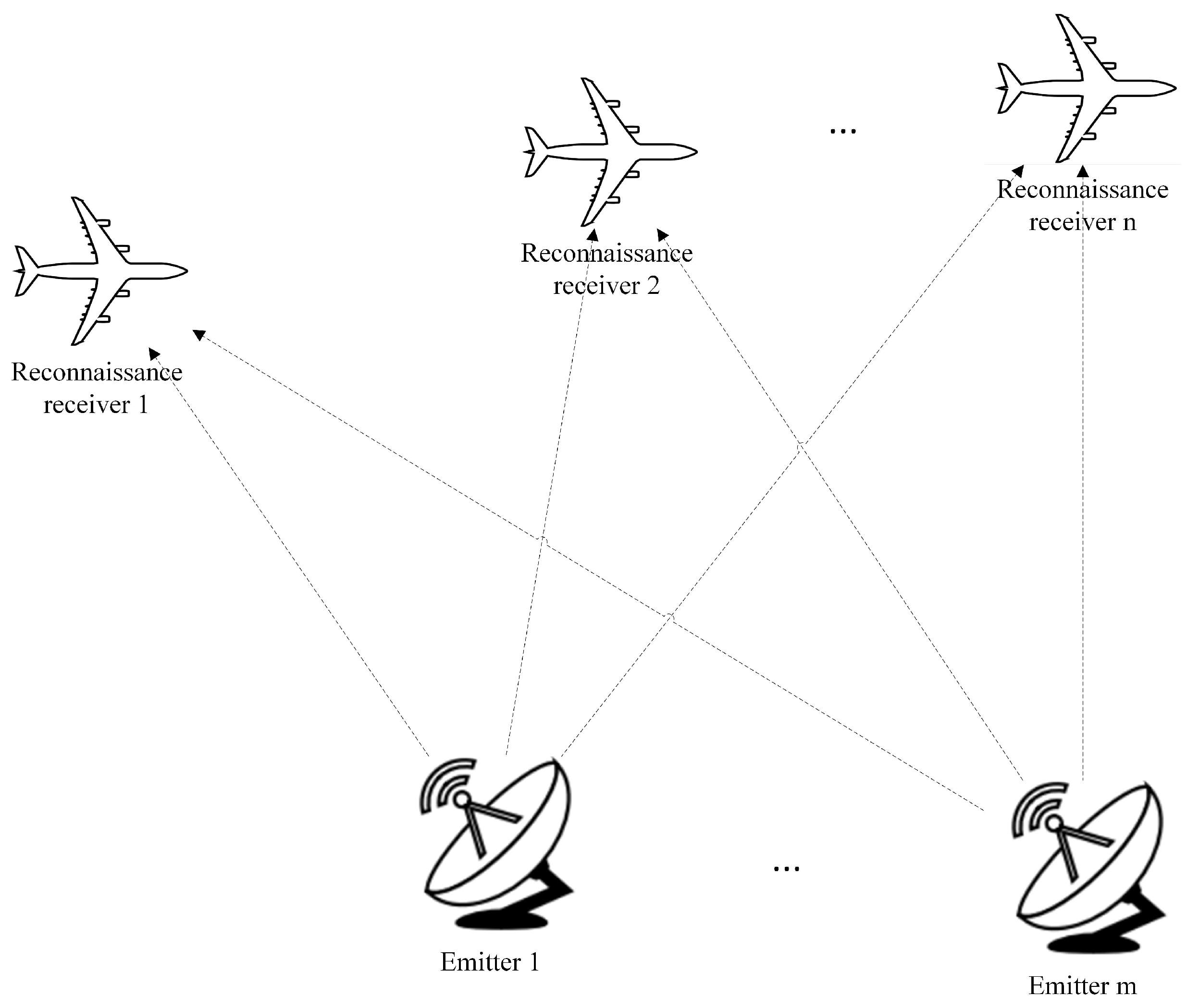
In a complex electromagnetic environment, the traditional signal detection and receiving mode of a single reconnaissance receiver proves inadequate for effectively detecting multiple emitters, thereby failing to meet the requirements of electronic warfare. To overcome this limitation, this paper performs a collaborative reconnaissance scene utilizing multiple receivers. By distributing the reconnaissance receivers, a broader reconnaissance range can be achieved, allowing for the collection of spatial dimensional data from diverse perspectives. Furthermore, the presence of redundant data can contribute to enhancing the accuracy of signal sorting.

The multi-receiver collaborative reconnaissance scene is shown in Figure 1, whose basic parameters are the following:

(a)

The number of receivers n ($n\ge 2$).

(b)

The number of emitters m ($m\ge 1$).

In detail, the setup is as follows. The space location of the multi-receiver needs to be processed before using it. In mathematics, a graph is a structure that describes a set of objects, where these objects are related to others in some sense. Graphs can be categorized as either undirected or directed, depending on whether the edges have specific directions. In the context of this study, undirected graphs are employed, as they consist of vertices (representing the receivers) and edges, making them straightforward to comprehend and implement. Moreover, undirected graphs are particularly suitable for this study, as the absence of directional edges accurately represents the bi-directional communication relationship between the receivers. Using a directed graph would necessitate the use of two edges to represent such a relationship, which would be cumbersome and unnecessary. Therefore, the use of a directed graph is unnecessary in this case.

To facilitate analysis, we assume that the communication among the receivers in the spatial domain can be represented by an undirected connected graph, denoted as $\mathcal{G}\left(t\right)=(\mathcal{V},\mathcal{E})$, where $\mathcal{V}=\{1,2,\dots ,n\}$ is the set of vertices, $\mathcal{E}$ is the set of edges, and t is a discrete time sequence. The positions of the vertices in the undirected graph reflect the horizontal distribution of the multi-receivers in physical space. The presence of an edge between two vertices indicates that the corresponding receivers are capable of exchanging information with each other. In practical scenarios, the topology of an undirected graph is typically determined by factors such as spatial distance and signal transmission power. These factors impose constraints on the connectivity among the receivers within the graph.

In this case, information exchange is limited to neighboring vertices within the undirected graph. Once the information is extracted from different receivers, it needs to be fused. This fusion process will be discussed in the subsequent section, where the mathematical theory of decision fusion will be introduced.

2.2. Mathematical Theory of D-S Evidence Theory

D-S evidence theory is widely recognized as one of the prominent methods for decision fusion. In this paper, the result of decision fusion is calculated using the orthogonal sum ⊕ defined within the framework of D-S evidence theory [28]. The mathematical theory and equations relevant to this study are presented below.

Considering such a finite identification framework $\Omega =\left\{e_1,e_2,\dots \dots .,e_n\right\}$, there are a total of $2^{\Omega }$ possible identification results. Each identification result is associated with a mass function that represents the confidence level of the receiver towards that specific result. This mapping of confidence levels is referred to as the basic belief assignment (BBA) or basic probability assignment (BPA), denoted as $m:2^{\Omega }\to [0,1]$

$$\left\{\begin{array}{c}\sum _{A\subseteq \Omega }m\left(A\right)=1\hfill \\ m(⌀)=0\hfill \end{array}\right.$$

(1)

If $m(⌀)\ne 0$, this BPA m was called subnormal. A subnormal BPA m can be made normalized $m^{\ast }$ through the following normalization operations:

$$m^{\ast }=\frac{m\left(A\right)}{1-m(⌀)}$$

(2)

for all $A\subseteq \Omega$, and $A\ne ⌀$.

Let $m_1$ and $m_2$ be two BPAs in the same framework $\Omega$, and let $m_{1\oplus 2}$ be a combination of orthogonal sum ⊕; thus,

$$m_{1\oplus 2}\left(A\right)=\left\{\begin{array}{cc}0\hfill & , A=⌀\hfill \\ \frac{{\displaystyle \sum _{B\cap C=A}}{m}_1\left(B\right)m_2\left(C\right)}{1-K}\hfill & ,\mathrm{else}\hfill \end{array}\right.$$

(3)

$$K=\sum _{B\cap C=⌀}{m}_1\left(B\right)m_2\left(C\right)$$

(4)

for all $A\subseteq \Omega$, where K is the degree of conflict between $m_1$ and $m_2$.

The combination rule defined by Equation (3) is known as Dempster’s combination rule. One notable characteristic of this rule is that it satisfies the exchange and commutative laws [28]. These properties imply that the order in which the evidence is combined does not impact the final result.

3. Information Fusion for Radar Signal Sorting with the Distributed Reconnaissance Receivers

This paper proposes an information fusion method for radar signal sorting with the distributed reconnaissance receivers, inspired by the distributed implementation strategy of fusion rules discussed in [15]. The fundamental premise of this method is that each reconnaissance receiver independently performs signal sorting and subsequently fuses these primary decisions to obtain the final decision. The method follows a decentralized approach, where the fusion process focuses on the sorting decision of the same single pulse across different receivers. By leveraging the distributed reconnaissance receivers, this method facilitates the effective fusion of sorting decisions collaboratively.

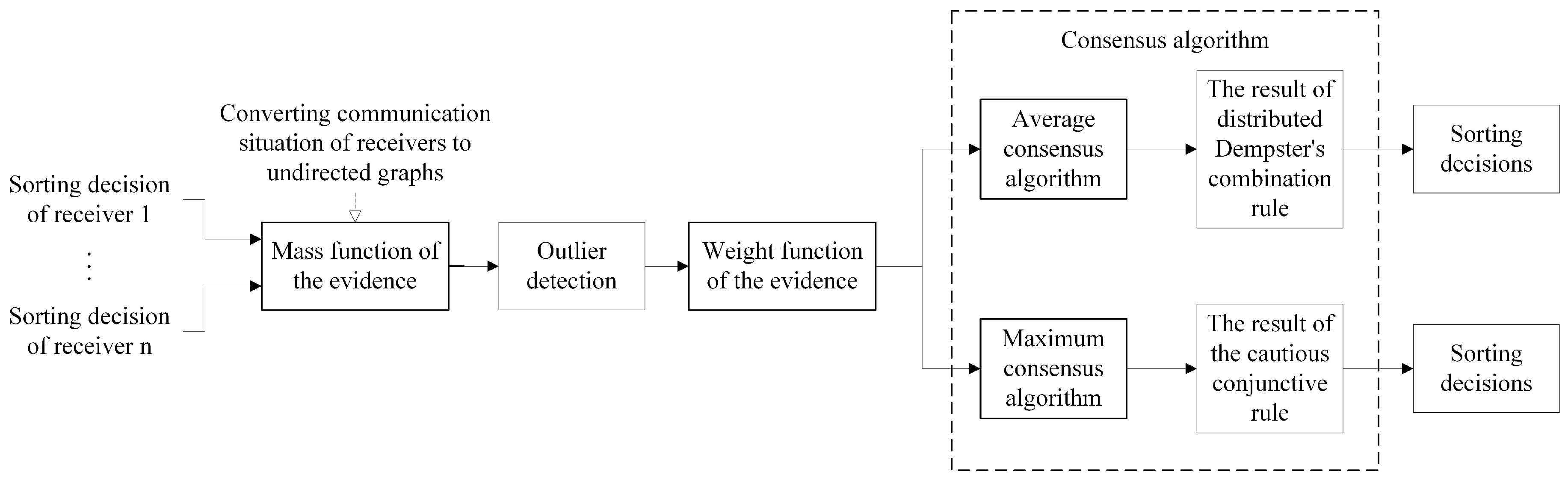
Figure 2 presents the flowchart depicting the process of distributed fusion. In this process, the sorting decisions made by the receivers are treated as evidence in the form of mass functions. To ensure the reliability of the fusion, an outlier detection algorithm is employed to eliminate any outliers present in the mass functions. Following this, the mass functions are transformed into weight functions.

Assuming that the receivers’ communication and spatial distribution can be represented by an undirected graph (refer to Section 2.1 System Scheme), each receiver holds a weight function during a single fusion. To achieve consensus among all receivers, the renewal equation of the consensus algorithm is utilized, enabling each receiver to obtain the same weight functions. Based on the expressions of Dempster’s combination rule and the cautious conjunctive rule under the weight form, they require the use of consensus algorithms to compute the summation and maximum value of the weights to achieve distributed fusion, respectively. Therefore, the average consensus algorithm and the maximum consensus algorithm are selected to implement the two fusion rules separately, resulting in the determination of sorting decisions under each respective fusion rule.

This approach ensures that the proposed method produces results equivalent to centralized fusion, while simultaneously enhancing the security and robustness of the information fusion process by eliminating the need for a central fusion center.

Each step in Figure 2 will be described in detail in the subsequent sections.

3.1. Mass Function of the Evidence

The first step in the fusion process involves extracting the information that needs to be fused. Assume a finite identification framework $\Omega =\left\{e_1,\dots ,e_m\right\}$, corresponding to different emitters. Each receiver i holds a mass function $m_i,i=1,2,\dots ,n$. The mass function represents the probabilities of the radar signal pulse belonging to each emitter $e_j,j=1,2,\dots ,m$. These probabilities are equivalent to the probabilities belonging to the corresponding sorting label.

To illustrate this, let us consider an identification framework $\Omega =\left\{e_1,e_2,e_3\right\}$. If we have a mass function $m=(0.7,0.2,0.1)$, it indicates that this radar pulse has a probability of 0.7 of belonging to $e_1$, a probability of 0.2 of belonging to $e_2$, and a probability of 0.1 of belonging to $e_3$.

Our objective is to design a distributed method that combines the mass functions of the receivers using Dempster’s combination rule and the cautious conjunctive rule.

3.2. Outlier Detection

In practical scenarios, it is common for some reconnaissance receivers to produce incorrect decisions due to various factors such as distance, interference, or errors in the pulse matching process. When erroneous information is present, directly fusing the data without considering the possibility of outliers can undermine the accuracy of the fusion results and may even introduce further errors.

To address this challenge, it is essential to incorporate an outlier detection process into the fusion method. The outlier detection algorithm helps identify and eliminate erroneous decisions or data points before performing the fusion. By detecting and removing outliers, the fusion process can be more robust and reliable.

In the context of electronic reconnaissance, the number of reconnaissance receivers is typically not as high as in big data scenarios, which means that conventional outlier detection algorithms designed for high data density may not be directly applicable. Instead, it is necessary to consider outlier detection algorithms specifically tailored for low data density situations.

In this paper, we have chosen the Connectivity-Based Outlier Factor (COF) as the initial outlier detection method for our distributed fusion approach. COF [29] is a variant of the Local Outlier Factor (LOF) algorithm, which is a classical density-based algorithm for outlier detection. LOF assesses the degree of outliers of each data point by considering the density of its neighbors.

The advantage of COF over LOF is its ability to handle outliers at low densities. COF calculates the local density based on the average chain distance. Initially, the algorithm determines the k-nearest neighbors of each data point. Then, to compute the distance vector $dist\left(e_i\right)$ between a point p and its k-nearest neighbors, where $i=1,2,\dots ,k$, we first construct the minimum spanning tree of the graph formed by point p and its neighboring points. Subsequently, the shortest path algorithm is executed, starting from point p to obtain the distance vector $dist\left(e_i\right)$. For example, if point a is the nearest neighbor of point p, point b is the nearest neighbor of point a, and point c is the nearest neighbor of point b, then the distance vector for the 3-nearest neighbors is formed by the distances between point p and point a, the distance between point a and point b, and the distance between point b and point c, in that order. Therefore, it is also referred to as the chain distance of point p.

Then the average chain distance of point p is

$$a{c}_{-}dist\left(p\right)=\sum _{i=1}^k\frac{2(k+1-i)}{k(k+1)}dist\left(e_i\right)$$

(5)

And, the COF of point p is

$$COF\left(p\right)=\frac{k·a{c}_{-}dist\left(p\right)}{{\sum }_{o\in N_k\left(p\right)}a{c}_{-}dist\left(o\right)}$$

(6)

The proposed outlier detection algorithm aims to leverage the feature that outliers are typically scattered, while inliers tend to form clusters to identify and correct errors in data. In the context of this algorithm, the outlier detection process can be applied to both the mass function and the weight function. However, the subsequent analysis reveals that the mass function tends to yield better results. This is primarily due to the difference in value ranges between the mass function and the weight function.

The mass function represents the probability of a radar signal pulse belonging to each emitter, and its values range from 0 to 1. On the other hand, the weight function is derived from the mass function and can have values ranging from 0 to infinity. When converting the mass function to the weight function, particularly when the mass function approaches 1, even numerically similar values in the mass function can lead to significant differences in the weight function. It is important to note that over-scattered values in the weight function can be unfavorable for outlier detection and may increase the probability of detection errors. Therefore, the outlier detection algorithm is primarily executed on the mass function.

Figure 3 presents the distributed outlier detection algorithm for the fusion of radar signal sorting with distributed reconnaissance receivers. This algorithm incorporates the Connectivity-Based Outlier Factor (COF) and employs confidence and distance calculations to identify inlier or outlier mass functions. Here is a breakdown of the steps involved:

Step 1. Calculate COF and confidence: For each receiver i with more than two neighbors $\left(\right|\mathcal{N}\left(i\right)|\ge 2)$, compute the COF and the confidence of COF for their mass functions. The value of k for $\mathrm{COF}$ is determined as $min\left(\left|\mathcal{N}\left(i\right)\right|,k_{max}\right)$, where $k_{max}$ is a chosen parameter to balance computational complexity. The confidence of COF is calculated using Equation (7), which quantifies the degree of confidence in the mass function.

$$\mathrm{confidence}=erf\left(\frac{\mathrm{COF}-{\mu }_{\mathrm{COF}}}{{\sigma }_{COF}^2}\right)$$

(7)

where $erf(·)$ is the error function.

Step 2. Label mass functions: Compare the confidence value with the COF threshold ${\tau }_{\mathrm{COF}}$. If the confidence is greater than ${\tau }_{\mathrm{COF}}$, the corresponding mass function is labeled as normal data; otherwise, it is labeled as abnormal data.

Step 3. Calculate center: Calculate the average of the mass functions labeled as normal data to obtain a center. Transmit this center to other receivers using the maximum consensus algorithm, ensuring that all receivers converge to the same center.

Step 4. Calculate distance: Each receiver calculates the distance between its mass function and the center. Transmit this distance to other receivers using the average consensus algorithm, allowing all receivers to obtain a consistent view of the distances.

Step 5. The sum of distances: Multiply the outcome of the average consensus algorithm by the total number of receivers n to obtain the sum of distances for each center.

Step 6. Identify the best center: Identify the best center by selecting the one with the minimum sum of distances. This center represents the most representative mass function among the receivers.

Step 7. Identify outliers: Each receiver compares the distance between its mass function and the best center with the distance threshold ${\tau }_{dist}$. If the distance is greater than ${\tau }_{dist}$, the corresponding mass function is labeled as an outlier; otherwise, it is labeled as an inlier.

It is worth noting that the quality of the center can be improved by increasing the threshold value of $\left|\mathcal{N}\left(i\right)\right|$. The values of the COF threshold ${\tau }_{\mathrm{COF}}$ and the distance threshold ${\tau }_{dist}$ can be determined experimentally, considering the specific characteristics of the data and the desired trade-off between the false positive rate and the false negative rate.

3.3. Weight Function of the Evidence

In an identification framework $\Omega$, the effect of evidence is typically expressed through the degree of support given to different hypotheses or subsets of $\Omega$. In some practical applications, the evidence may explicitly indicate a single non-empty subset A of $\Omega$ as the most likely hypothesis. Mathematically, this situation can be simplified by using a simple support function, also known as a special form of the mass function

$$m\left(A\right)=s,m(\Omega )=1-s$$

(8)

Let $m_1$ and $m_2$ be two simple support functions for the same non-empty set A, respectively, with support $s_1$ and $s_2$, and let $m_{1\oplus 2}$ be a combination of orthogonal sum ⊕; then, we have

$$\begin{array}{cc}\hfill & m_{1\oplus 2}\left(A\right)=1-(1-s_1)(1-s_2)\hfill \\ \hfill & m_{1\oplus 2}(\Omega )=(1-s_1)(1-s_2)\hfill \end{array}$$

(9)

Degrees of support are frequently linked to the weights of evidence. Shafer [28] defines the weight form of the evidence $A^{\omega }$, where A in $A^{\omega }$ refers to a non-empty subset supported by the evidence, and the superscript $\omega$ denotes the evidence weights defined by Equation (10). For the simple support function, its transformation with the weight form of the evidence is represented as follows:

$$s=1-e^{-\omega },\omega =-log(1-s)$$

(10)

$$m\left(A\right)=1-e^{-\omega },m(\Omega )=e^{-\omega }$$

(11)

3.3.1. Weight Form of Dempster’s Combination Rule

After getting the weight form of the evidence, the orthogonal sum of the weight $A^{\omega }$ between the simple support function $m_1$ and $m_2$ becomes the following form:

$$A^{{\omega }_1}\oplus A^{{\omega }_2}=A^{{\omega }_1+{\omega }_2}$$

(12)

If a mass function is a simple support function or is equal to the orthogonal sum of two or more simple support functions, it is called a separable support function:

$$m=\underset{⌀\ne A\subseteq \Omega }{\oplus }{A}^{\omega \left(A\right)}$$

(13)

where $\omega \left(A\right)$ is the weight of evidence for the subset A.

According to Equations (12) and (13), the weight form of Dempster’s combination rule is expressed as follows:

$$m_{1\oplus 2}=\underset{⌀\ne A\subseteq \Omega }{\oplus }{A}^{{\omega }_1\left(A\right)+{\omega }_2\left(A\right)}$$

(14)

3.3.2. Weight Form of Cautious Conjunctive Rule

Assume that we have two sources of information that provide BPA $m_1$ and $m_2$, and that both sources are considered reliable. After receiving these two messages, the receiver’s belief status should be represented by the BBA $m_{12}$, which contains more abundant information than $m_1$ and $m_2$. Let us denote the set of information by $S\left(m\right)$, so we have $m_{12}\in S\left(m_1\right)$ and $m_{12}\in S\left(m_2\right)$, or equivalently, $m_{12}\in S\left(m_1\right)\cap S\left(m_2\right)$.

Let $m_1$ and $m_2$ be two BPAs; the cautious conjunctive rule is defined by the following [30]:

$${\omega }_{1\wedge 2}\left(A\right)={\omega }_1\left(A\right)\wedge {\omega }_2\left(A\right)$$

(15)

for all $A\subseteq \Omega$, where ∧ denotes the minimum operator.

According to Equations (13) and (15), the weight form of the cautious conjunctive rule is expressed as follows:

$$m_{1\wedge 2}=\underset{⌀\ne A\subseteq \Omega }{\oplus }{A}^{{\omega }_1\left(A\right)\wedge {\omega }_2\left(A\right)}$$

(16)

Equation (16) is modified to avoid zero weight under high evidence conflict as follows:

$$m_{1\vee 2}=\underset{⌀\ne A\subseteq \Omega }{\oplus }{A}^{{\omega }_1\left(A\right)\vee {\omega }_2\left(A\right)}$$

(17)

where ∨ denotes the maximum operator.

According to Equations (14) and (17), the sum and maximum method can be used to achieve a distributed implementation of the weight form of Dempster’s combination rule and the cautious conjunctive rule, respectively.

3.4. Consensus Algorithm

There are two possible methods for the distributed implementation of weight combinations: The first method is flooding [22], which involves each receiver broadcasting all the data it holds to its neighboring receivers. This means that each receiver will receive data from its neighbors and save all the received data. Ultimately, each receiver possesses all the data. However, this method requires a significant amount of data throughput, especially when the number of receivers is large. The second method is the consensus protocol [20]. Instead of broadcasting and storing all the data, each receiver updates its own data using the information broadcasted by its neighboring receivers. The receivers iteratively exchange and update their data until convergence is achieved, at which point all receivers will have the same data. This approach requires minimal data throughput but takes time for the data to converge.

In the latter approach of using the consensus protocol for the distributed implementation of weight combinations, the combination of evidence weights can be abstracted as a consensus problem. Specifically, two types of consensus problems arise: the summation consensus problem and the maximum consensus problem. Notably, the summation consensus problem can be transformed into the average consensus problem.

This paper solely focuses on the static consensus problem, which involves receivers acquiring the mass function and then combining it with the mass functions of other receivers. In contrast, the dynamic consensus problem [31] involves receivers not only exchanging information with each other, but also continuously acquiring information from the external environment. In the context of distributed reconnaissance and the focus on decision fusion for radar signal sorting, this paper is concerned with the static consensus problem.

Let each receiver i in the undirected graph have an initial value $x_i\left(0\right)$ at $t=0$. The receivers update their state at discrete times $t=1,2,\dots$ using the renewal equation. This equation allows the states of all receivers to converge to the same value over time. The renewal equation, as described in [20], is given by

$$x(t+1)=W\left(t\right)x\left(t\right)$$

(18)

$$x_i(t+1)=\sum _{j=1}^n{w}_{ij}\left(t\right)x_j\left(t\right)$$

(19)

where $x\left(t\right)={(x_1\left(t\right),x_2\left(t\right),\dots ,x_n\left(t\right))}^T$, $W\left(t\right)\in {\mathbb{R}}^{n\times n}$ is the weight matrix and $W\left(t\right)$ is usually a symmetric matrix in undirected graphs.

Theorems 3.1 and 3.2 in [20] confirm that undirected graphs exhibit convergence when their topology remains fixed and the matrix $W\left(t\right)$ is constant. Even when the topology of an undirected graph changes over time, convergence can still be guaranteed as long as the topology remains connected at all points in time.

3.4.1. Average Consensus

The average consensus aims to converge to the average of all initial values $x_i\left(0\right)$ by utilizing the renewal equation. In previous studies [32,33,34], the Metropolis–Hastings algorithm (M–H) [35] has been widely applied as a weight model in distributed average consensus-based algorithms for data aggregation. A variant of the M–H algorithm known as the generalized Metropolis–Hastings weight model (GMH) [36] is particularly useful. The GMH weights offer the advantage of being easy to compute and requiring only local information about the graph topology.

The weight matrix of the GMH can be defined as follows [36]:

$$w_{ij}^{GMH}=\left\{\begin{array}{cc}1-{\sum }_{i\ne j}{w}_{ij}^{GMH}\hfill & , \mathrm{if}i=j\hfill \\ \frac{1}{max\left\{d_i,d_j\right\}+ϵ}\hfill & , \mathrm{if}(i,j)\in \mathcal{E}\hfill \\ 0\hfill & , otherwise\hfill \end{array}\right.$$

(20)

where $ϵ$ is the mixing parameter, and $d_i$ is the degree of the corresponding vertex i; the degree $d_i$ of the vertex i equals the number of its neighbors.

It is important to note that the convergence result can be considered errorless after rounding if the convergence accuracy is at least one bit higher than the expected result. The parameter $ϵ$ and convergence accuracy can be determined experimentally. The average consensus algorithm using Equations (19) and (20) provides the average value of the receivers’ weight function. According to Equation (14), it can be observed that the orthogonal sum (i.e., Dempster’s combination rule) of the mass functions $m_1$ and $m_2$, supporting the same non-empty set A, is the sum of their respective weights. The average consensus algorithm, on the other hand, computes the average of all participating weights during the transmission process. Multiplying this average by the number of vertices yields the sum of weights. In order to apply Dempster’s combination rule, which involves summing the weights of evidence, it is necessary to know the total number of vertices n in the undirected graph.

If the number of vertices is known, the sum of the weights can be obtained by multiplying the convergence result (average weight) with n. However, if the number of vertices is unknown, an estimation method can be used. In this method, the initial value of the first vertex is set to 1, while the initial values of the remaining vertices are set to 0, i.e., $x\left(0\right)={(1,0,\dots ,0)}^T$. By applying the average consensus algorithm to these initial values, the convergence result will be $1/n$. Taking the reciprocal of this result gives the estimated value of n. Therefore, multiplying the average weight by the total number of vertices n provides the sum of the weights.

3.4.2. Maximum Consensus

The maximum consensus aims to converge to the maximum value among all initial values $x_i\left(0\right)$ by utilizing the renewal equation. Unlike the average consensus, the maximum consensus does not involve a weight matrix and relies solely on information from neighboring vertices. The renewal equation in Equation (19) is rewritten into the following form

$$x_i(t+1)=\underset{j\in \left\{i\right\}\cup \mathcal{N}\left(i\right)}{max}{x}_j\left(t\right)$$

(21)

where $\mathcal{N}\left(i\right)$ denotes the adjacent vertex set of i.

4. Computer Simulation

4.1. Fusion Rule Demonstration and Convergence Performance Analysis

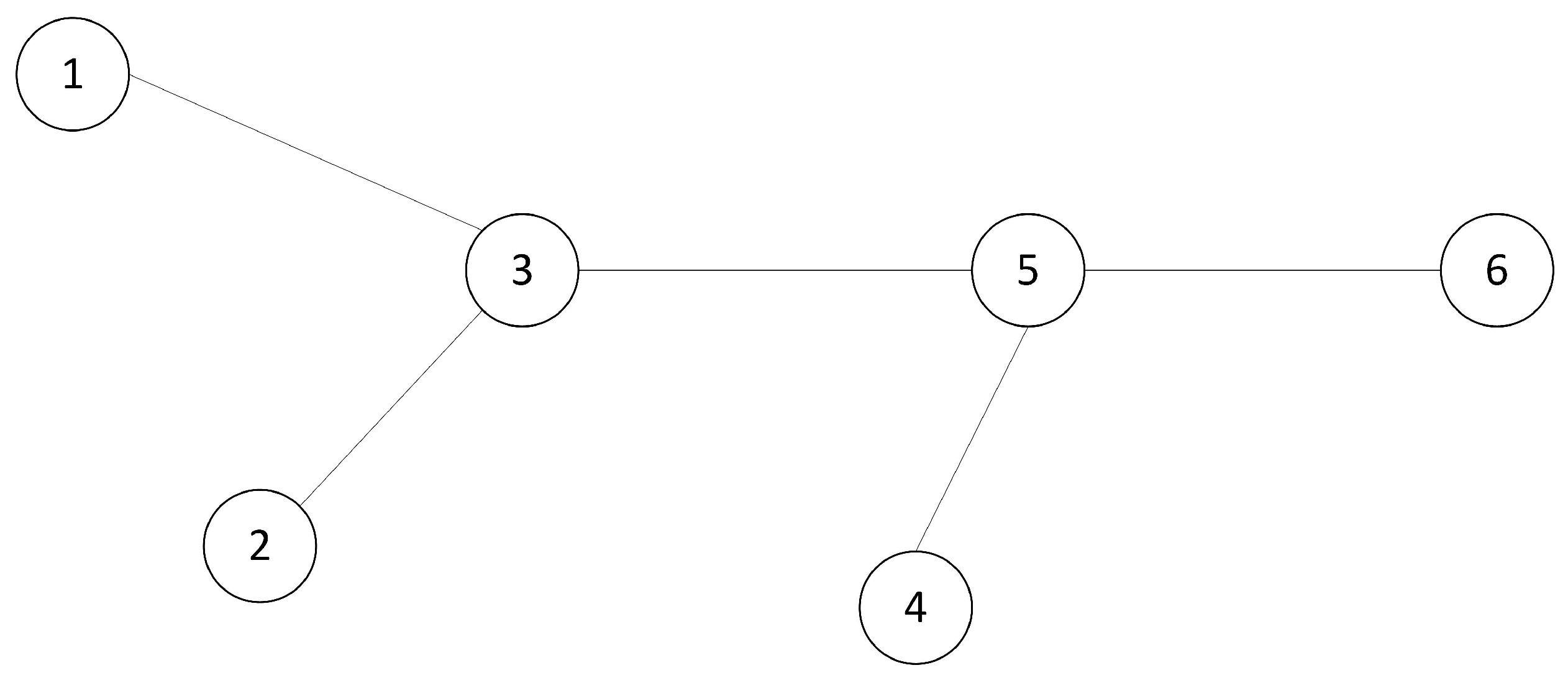
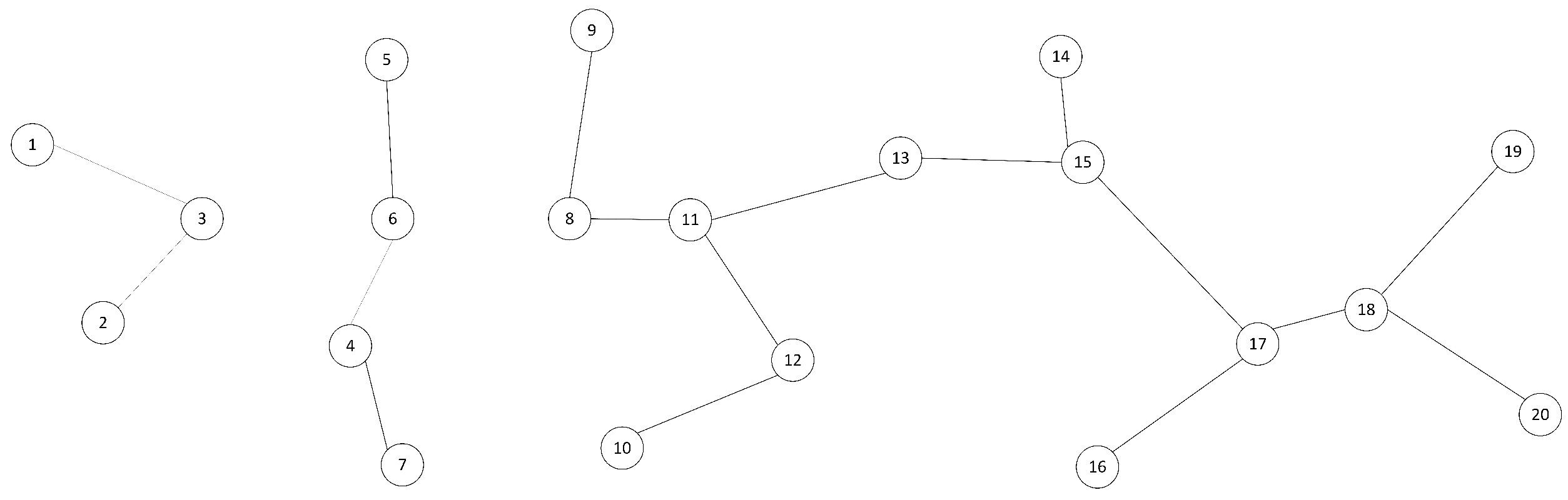
After following the guidelines outlined in Section 3, we consider a topology of an undirected graph with low connectivity, as depicted in Figure 4.

The number of receivers is denoted as $n=6$, and we assume a finite identification framework $\Omega =\left\{e_1,e_2,e_3,e_4,e_5\right\}$, representing five different emitters. The mass functions of the evidence are derived from the independent radar signal sorting results obtained by each receiver, as presented in

Table 1. The mass functions of the evidence.

	$\left\{{\mathit{e}}_1\right\}$	$\left\{{\mathit{e}}_2\right\}$	$\left\{{\mathit{e}}_3\right\}$	$\left\{{\mathit{e}}_4\right\}$	$\left\{{\mathit{e}}_5\right\}$
$m_1$	0.7	0.2	0	0.1	0
$m_2$	0.6	0.1	0.2	0	0.1
$m_3$	0.8	0	0	0	0.2
$m_4$	0.7	0	0.2	0	0.1
$m_5$	0	0.2	0.7	0	0.1
$m_6$	0	0.1	0.1	0.6	0.2

.

According to Equations (10) and (11), the mass functions of the evidence in Table 1 is transformed into weights of the evidence, as shown in

Table 2. The weights of the evidence.

	$\left\{{\mathit{e}}_1\right\}$	$\left\{{\mathit{e}}_2\right\}$	$\left\{{\mathit{e}}_3\right\}$	$\left\{{\mathit{e}}_4\right\}$	$\left\{{\mathit{e}}_5\right\}$
${\omega }_1$	1.2	0.2	0	0.1	0
${\omega }_2$	0.9	0.1	0.2	0	0.1
${\omega }_3$	1.6	0	0	0	0.2
${\omega }_4$	1.2	0	0.2	0	0.1
${\omega }_5$	0	0.2	1.2	0	0.1
${\omega }_6$	0	0.1	0.1	0.9	0.2

. The data in Table 2 provides further support for the subsequent calculation of fusion rules.

4.1.1. Combination by the Cautious Conjunctive Rule

By employing Equation (21) to update the weights of the evidence in Table 2, the weights converge in three iterations to the weight vector ${\omega }_{\vee }=(1.6,0.2,1.2,0.9,0.2)$, which corresponds to the following mass function:

$$m_{\vee }={\left\{e_1\right\}}^{1.6}\oplus {\left\{e_2\right\}}^{0.2}\oplus {\left\{e_3\right\}}^{1.2}\oplus {\left\{e_4\right\}}^{0.9}\oplus {\left\{e_5\right\}}^{0.2}$$

Further calculation gives

$$\begin{array}{cc}& m_{\vee }\left\{e_1\right\}=0.48713,m_{\vee }\left\{e_2\right\}=0.03838,m_{\vee }\left\{e_3\right\}=0.33830,m_{\vee }\left\{e_4\right\}=0.17953,\hfill \\ & m_{\vee }\left\{e_5\right\}=0.02673.\hfill \end{array}$$

In $m_{\vee }={\left\{e_1\right\}}^{1.6}\oplus {\left\{e_2\right\}}^{0.2}\oplus {\left\{e_3\right\}}^{1.2}\oplus {\left\{e_4\right\}}^{0.9}\oplus {\left\{e_5\right\}}^{0.2}$, there are five subsets that require four orthogonal sum operations. For example, let us consider the first orthogonal sum calculation step:

$$\begin{array}{cc}& m_1\left\{e_1\right\}=1-e^{-1.6}\approx 0.80,m_2\left\{e_2\right\}=1-e^{-0.2}\approx 0.18\hfill \\ & m_1\{\Omega \}=-e^{-1.6}\approx 0.20,m_2\{\Omega \}=-e^{-0.2}\approx 0.82\hfill \end{array}$$

$$\begin{array}{cc}& \therefore m_{1\oplus 2}\left\{e_1\right\}=\frac{0.80\times 0.82}{1-0.80\times 0.18}\approx 0.77,m_{1\oplus 2}\left\{e_2\right\}=\frac{0.20\times 0.18}{1-0.80\times 0.18}\approx 0.04,\hfill \\ & m_{1\oplus 2}\{\Omega \}=\frac{0.20\times 0.82}{1-0.80\times 0.18}\approx 0.19\hfill \end{array}$$

4.1.2. Combination by Dempster’s Combination Rule

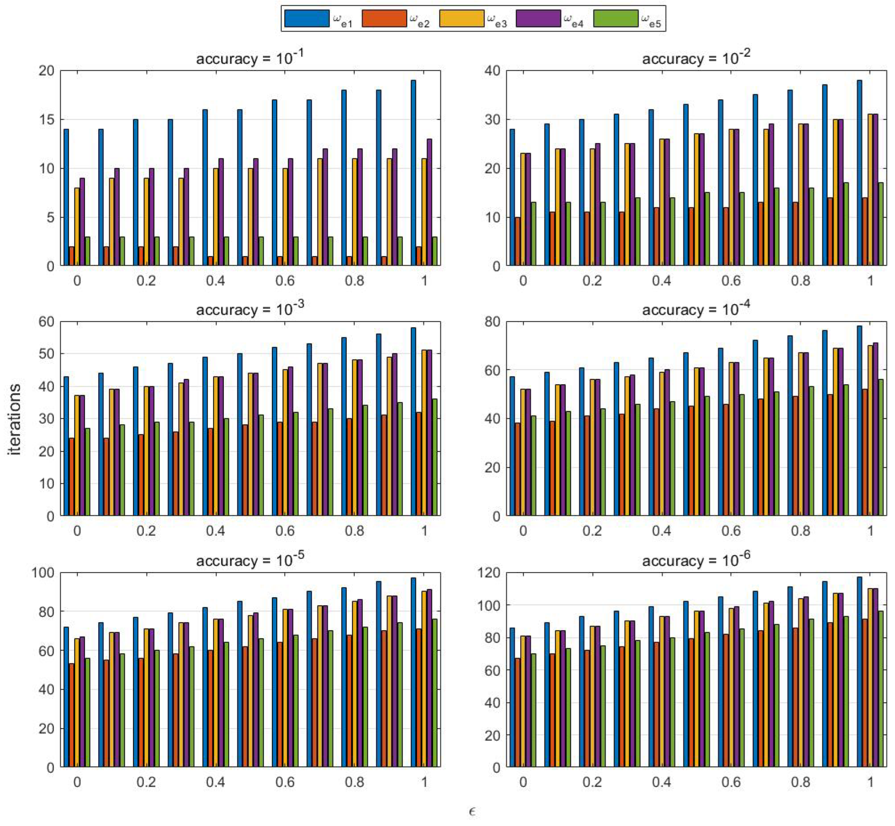
The effects of convergence accuracy and parameter $ϵ$ on convergence speed in Equation (20) are considered here. The convergence accuracy is set to [${10}^{-1}$, ${10}^{-2}$, ${10}^{-3}$, ${10}^{-4}$, ${10}^{-5}$, ${10}^{-6}$], and the parameter $ϵ$ ranges from 0 to 1 with a scale of 0.1. The convergence speeds for different combinations are shown below.

Figure 5 illustrates the impact of convergence accuracy, parameter $ϵ$, and the numerical difference in the initial values on the convergence speed of the algorithm. With $ϵ=0$, the algorithm achieves the fastest convergence speed. As the parameter $ϵ$ increases, the number of iterations required for convergence gradually increases. Additionally, the convergence speed is fastest when the convergence accuracy is set to ${10}^{-1}$, and it gradually decreases as the convergence accuracy becomes higher. Furthermore, the initial values of convergence also play a role in the convergence speed. When the initial values differ significantly, such as in the case of ${\omega }_{e1}$, the convergence speed is notably slower compared to cases with smaller initial value differences, such as ${\omega }_{e2}$ and ${\omega }_{e5}$. Although not explicitly shown in Figure 5, it is worth noting that the number of vertices in the graph topology also impacts the convergence speed. Generally, a larger number of vertices results in a slower convergence speed.

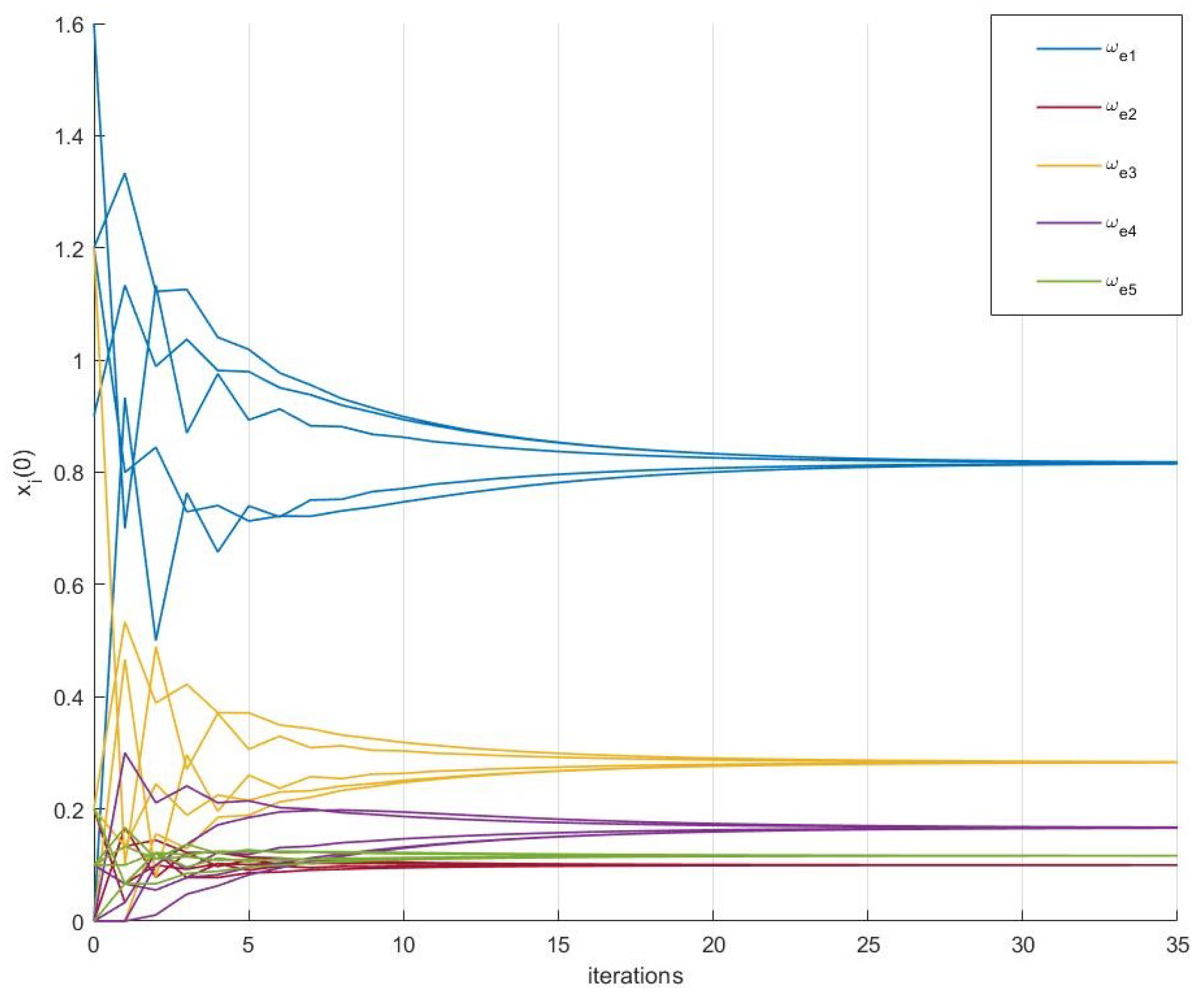
Based on the chosen parameters $ϵ=0$ and the convergence accuracy of ${10}^{-2}$, the results of the average consensus algorithm are shown in Figure 6. The average consensus algorithm using Equations (16) and (17) gives the average weight value ${\overline{\omega }}_{\sum }=(0.8213,0.1048,0.2789,0.1621,0.1124)$ for the evidence in Table 2. The convergence result of the vertices’ estimation method described in Section 3.4 is 0.1716. Thus, the number of reconnaissance receivers can be calculated as $n=round\left(\frac{1}{0.1716}\right)=6$, which matches the actual number. Finally, the sum of the weights is computed as ${\omega }_{\sum }={\overline{\omega }}_{\sum }\times n=(4.9,0.6,1.7,1.0,0.7)$, which corresponds to the following mass function:

$$m_{\oplus }={\left\{e_1\right\}}^{4.9}\oplus {\left\{e_2\right\}}^{0.6}\oplus {\left\{e_3\right\}}^{1.7}\oplus {\left\{e_4\right\}}^{1.0}\oplus {\left\{e_5\right\}}^{0.7}$$

further calculation gives

$$\begin{array}{cc}& m_{\oplus }\left\{e_1\right\}=0.92457,m_{\oplus }\left\{e_2\right\}=0.00799,m_{\oplus }\left\{e_3\right\}=0.04323,m_{\oplus }\left\{e_4\right\}=0.01605,\hfill \\ & m_{\oplus }\left\{e_5\right\}=0.00934.\hfill \end{array}$$

By calculating the two combination rules mentioned above, it becomes evident that Dempster’s combination rule provides higher support for the correct emitter compared to the cautious conjunctive rule. However, the cautious conjunctive rule may be more effective for fusion involving multiple subsets (i.e., $\left|A\right|\ge 2$), but it exhibits caution when dealing with high-conflict single subset fusion (i.e., $\left|A\right|=1$). Additionally, the cautious conjunctive rule achieves convergence in just a few iterations, whereas Dempster’s combination rule requires a minimum of 27 iterations to converge.

4.2. Method Comparison and Analysis

The performance of the proposed outlier detection algorithm is analyzed based on the topology of the undirected graph depicted in Figure 7. The graph consists of 20 receivers, and the identification framework is represented by $\Omega =\left\{e_1,e_2,e_3,e_4,e_5\right\}$.

4.2.1. Influence of Outlier Detection Algorithm’s Parameters

To observe the effect of parameter selection on the algorithm, the single reconnaissance receiver sorting accuracy is set to 50%. This implies that there are n multiple accuracy reconnaissance receivers, where the maximum value of the mass function corresponds to the correct emitter, and the remaining values correspond to incorrect emitters. In each experiment, 500 Monte Carlo experiments were conducted with k = 20, and the mass functions of all reconnaissance receivers were randomized. The instances where reconnaissance receiver sorting appears incorrect and the sorting result of erroneous emitters are both determined randomly.

The effects of ${\tau }_{\mathrm{COF}}$ and ${\tau }_{dist}$ on the false positive rate and false negative rate were investigated. We considered the values of ${\tau }_{\mathrm{COF}}\in \left\{0.1,0.2,0.3,0.4,0.5,0.6,0.7,0.8,0.9\right\}$ and ${\tau }_{dist}\in \left\{0.1,0.2,0.3,0.4,0.5,0.6,0.7,0.8,0.9\right\}$.

Table 3. False positive rates (a) and false negative rates (b) in % of the outlier detection algorithm with different values of parameters ${\tau }_{\mathrm{COF}}$ and ${\tau }_{dist}$.

(a) False positive rate
		${\tau }_{dist}$
		0.1	0.2	0.3	0.4	0.5	0.6	0.7	0.8	0.9
${\tau }_{\mathrm{COF}}$	0.1	47.17	42.05	36.97	35.74	26.91	17.85	6.7	1.87	0.72
	0.2	46.98	38.39	33.39	31.59	28.59	21.74	8.47	1.74	0.13
	0.3	47.03	37.08	31.43	29.28	28.15	22.53	8.92	1.45	0.15
	0.4	44.34	24.19	11.7	10.07	8.52	7.1	3.99	1.83	0.97
	0.5	44.31	22.12	9.27	5.19	5.97	4.11	2.99	1.64	0.79
	0.6	44.35	22.79	9.22	5.44	4.79	4.75	3.89	2.46	1.33
	0.7	43.91	21.16	7.37	4.3	4.76	3.92	2.65	1.53	0.99
	0.8	43.9	22.19	7.82	4.06	4.29	3.68	2.59	2.18	1.62
	0.9	42.96	20.13	8.09	3.47	4.39	3.82	2.23	1.45	1.62
(b) False negative rate
		${\tau }_{dist}$
		0.1	0.2	0.3	0.4	0.5	0.6	0.7	0.8	0.9
${\tau }_{\mathrm{COF}}$	0.1	0	0	0	0	0.1	0.28	2.22	7.71	15.85
	0.2	0.02	0	0	0	0.13	0.23	2.21	8.83	18.69
	0.3	0	0	0.08	0.09	0	0.44	2.31	9.39	19.1
	0.4	0.07	0.21	0.16	0.48	0.75	1.02	1.91	3.38	4.06
	0.5	0.02	0.12	0.39	0.32	0.59	0.85	1.71	2.54	3.1
	0.6	0.03	0.31	0.48	0.34	0.79	1.53	1.85	3.17	2.69
	0.7	0.06	0.16	0.46	0.54	0.81	1.28	1.47	1.89	2.89
	0.8	0.04	0.39	0.53	0.31	0.96	0.77	1.72	2.64	3.07
	0.9	0.03	0.29	0.61	0.7	0.8	1.32	1.16	1.63	2.09

presents the average percentage of the false positive rate (proportion of inliers incorrectly marked as outliers, Table 3a) and false negative rate (proportion of outliers incorrectly marked as inliers, Table 3b) based on the 500 Monte Carlo experiments.

As the parameter ${\tau }_{dist}$ increases, the false positive rate decreases while the false negative rate increases. On the other hand, the effect of the parameter ${\tau }_{\mathrm{COF}}$ on program performance was divided into two bands [0.1, 0.3] and [0.4, 0.9]. Within these ranges, there was little change in performance, but there was a significant decrease in performance between [0.3, 0.4]. Parameters ${\tau }_{\mathrm{COF}}$ and ${\tau }_{dist}$ with values in the [0.4, 0.9] and [0.4, 0.7] ranges appear to yield good results.

4.2.2. Influence of Sorting Accuracy of Single Reconnaissance Receiver

The single reconnaissance receiver sorting accuracies were set to 90%, 80%, 70%, 60%, and 50%, respectively. A total of 500 Monte Carlo experiments were conducted with $k=20$, ${\tau }_{\mathrm{COF}}=0.5$, and ${\tau }_{dist}=0.4$. The sorting accuracies of the fusion process, both with and without the outlier detection algorithm, were evaluated under different single reconnaissance receiver sorting accuracies. The results are presented in

Table 4. The sorting accuracy of the fusion process using outlier detection algorithm under different sorting accuracies of a single reconnaissance receiver.

		Sorting Accuracy of a Single Reconnaissance Receiver
		90%	80%	70%	60%	50%
Fusion rule	C	100%	100%	100%	100%	97.40%
	D	100%	100%	100%	100%	97.60%

and

Table 5. The sorting accuracy of the fusion process without using an outlier detection algorithm under different sorting accuracies of a single reconnaissance receiver.

		Sorting Accuracy of a Single Reconnaissance Receiver
		90%	80%	70%	60%	50%
Fusion rule	C	69.00%	44.60%	32.00%	24.60%	14.40%
	D	92.40%	56.80%	17.20%	0.80%	0%

, where the cautious conjunctive rule is abbreviated as C, and Dempster’s combination rule is abbreviated as D.

After the individual reconnaissance receivers perform signal sorting independently, their preliminary decisions are fused. In this analysis, outlier detection algorithms are employed during the fusion process. The results indicate that when the sorting accuracy of a single reconnaissance receiver is equal to or higher than 60%, both fusion rules achieve a sorting accuracy of 100%. Even when the sorting accuracy of a single reconnaissance receiver is as low as 50%, the fused result still maintains a sorting accuracy of over 97%. On the other hand, without the use of outlier detection algorithms during the fusion process, sorting failures are more common, mainly attributed to unhandled conflicting information in the data.

The utilization of outlier detection algorithms during the fusion process proves to be effective in mitigating sorting errors that may arise due to the low sorting accuracy of individual reconnaissance receivers. This approach significantly enhances the overall accuracy of radar signal sorting. By identifying and excluding outliers, the fusion process can effectively filter out erroneous or conflicting information, leading to more reliable and accurate results.

Due to the limited number of published studies on distributed fusion algorithms at present, three typical centralized fusion algorithms were selected to facilitate a comparative analysis with the proposed algorithm in this paper. The sorting accuracy achieved after applying these three typical fusion algorithms under the same simulation conditions is presented in

Table 6. The sorting accuracy of the fusion process using typical fusion algorithms under different sorting accuracies of a single reconnaissance receiver.

		Sorting Accuracy of a Single Reconnaissance Receiver
		90%	80%	70%	60%	50%
Fusion rule	Dempster [28]	38.60%	15.00%	5.80%	2.50%	1.00%
	Murphy [37]	100%	100%	100%	100%	97.00%
	Deng [38]	100%	100%	100%	100%	97.20%

.

Based on the comparison between Table 4 and Table 6, it can be observed that the proposed method achieves the highest sorting accuracy under different sorting accuracies of a single reconnaissance receiver. Although the improvement of the proposed method over the Murphy algorithm and the Deng algorithm is only 0.6% and 0.4%, respectively, when the sorting accuracies of a single reconnaissance receiver is 50%, it should be noted that the proposed method is implemented through distributed fusion, while both the Murphy algorithm and the Deng algorithm are centralized fusion algorithms that require significant communication requirements among the receivers. This contributes to the enhanced effectiveness and superiority of the proposed method.

5. Conclusions

To overcome the distance limitations associated with centralized fusion and to address concerns related to the security and reliability of the fusion process, we propose a novel distributed information fusion method for radar signal sorting with distributed reconnaissance receivers. Furthermore, we propose a novel outlier detection algorithm within the fusion process to enhance its robustness. Experimental results demonstrate that even if the sorting accuracy of a single receiver is as low as 50%, the proposed distributed information fusion method can significantly improve the accuracy of radar signal sorting. It is worth noting that in this paper, our focus is solely on the issue of synchronous fusion. Further research can explore how to design fusion algorithms that can adapt to asynchronous environments in order to achieve accurate results. In such cases, fusion algorithms need to handle time differences between receiver data and communication instability. Additionally, we also consider the potential integration of intelligent methods into the fusion process to further enhance its robustness. For example, machine learning models can be employed to model and predict data, thereby improving the performance of fusion algorithms. Furthermore, the application of reinforcement learning methods in the fusion process can enable the system to make optimized decisions based on real-time environmental conditions and task requirements.

References

- Coluccia, A.; Fascista, A.; Ricci, G. Design of Customized Adaptive Radar Detectors in the CFAR Feature Plane. IEEE Trans. Signal Process. 2022, 70, 5133–5147. [Google Scholar] [CrossRef]
- Pietkiewicz, T. Removal of conflicts in fusion of identification information from ELINT-ESM sensors. In Proceedings of the XII Conference on Reconnaissance and Electronic Warfare Systems, Ołtarzew, Poland, 19–21 November 2018; SPIE: Bellingham, WA, USA, 2019; Volume 11055. [Google Scholar] [CrossRef]
- Wan, L.; Liu, R.; Sun, L.; Nie, H.; Wang, X. UAV swarm based radar signal sorting via multi-source data fusion: A deep transfer learning framework. Inf. Fusion 2022, 78, 90–101. [Google Scholar] [CrossRef]
- Zhang, L.; Xie, Y.; Xidao, L.; Zhang, X. Multi-source heterogeneous data fusion. In Proceedings of the 2018 International Conference on Artificial Intelligence and Big Data, ICAIBD 2018, Chengdu, China, 26–28 May 2018; Institute of Electrical and Electronics Engineers Inc.: New York, NY, USA, 2018; pp. 47–51. [Google Scholar] [CrossRef]
- Ge, J.; Wang, H.; Liu, G.; Lv, W. The Design and Implementation of Multi-radar Signal-level Cooperative Detection System. In Proceedings of the 2021 CIE International Conference on Radar (Radar), Haikou, China, 15–19 December 2021; pp. 2636–2640. [Google Scholar] [CrossRef]
- He, K.; Liu, X.; Liu, Y.; Guo, R.; Guo, K. A Joint Radar Signal Sorting Method For Multi-radar Reconnaissance Station. In Proceedings of the 3rd International Conference on Electrical, Mechanical and Computer Engineering, Guizhou, China, 9–11 August 2019; IOP Publishing: Bristol, UK, 2019; Volume 1314. [Google Scholar] [CrossRef]
- Liu, K.; He, M.; Han, J.; Feng, M.; Du, X. Data fusion algorithm for radar countermeasures and reconnaissance based on multi-sensor. Xi Tong Gong Cheng Yu Dian Zi Ji Shu/Syst. Eng. Electron. 2023, 45, 101–107. [Google Scholar] [CrossRef]
- Tortora, S.; Sindico, A.; Severino, G. A data fusion architecture for an Electronic Warfare multi-sensor suite. In Proceedings of the 2010 2nd International Workshop on Cognitive Information Processing, CIP2010, Elba Island, Italy, 14–16 June 2010; IEEE Computer Society: Washington, DC, USA, 2010; pp. 29–34. [Google Scholar] [CrossRef]
- Wang, D.; Zhang, J.; Zheng, S. Multi-source Information Data Fusion Method under Complex Battlefield Situation. In Proceedings of the 2nd International Conference on Artificial Intelligence and Computer Science, AICS 2020, Hangzhou, China, 25–26 July 2020; IOP Publishing Ltd.: Bristol, UK, 2020; Volume 1631. [Google Scholar] [CrossRef]
- Wang, J.; Wang, X.; Zhou, Y.; Chen, Y. Radar Emitter Classification Based on a Multiperspective Collaborative Clustering Method and Radar Characteristic Spectrum. Int. J. Aerosp. Eng. 2022, 2022, 1297735. [Google Scholar] [CrossRef]
- Zihao, Z.; Huaguo, Z.; Lu, G. A multi-station signal sorting method based on TDOA grid clustering. In Proceedings of the 2021 IEEE 6th International Conference on Signal and Image Processing (ICSIP), Nanjing, China, 22–24 October 2021; pp. 773–778. [Google Scholar] [CrossRef]
- Fuyuan, X. Multi-sensor data fusion based on the belief divergence measure of evidences and the belief entropy. Inf. Fusion 2019, 46, 23–32. [Google Scholar] [CrossRef]
- Braca, P.; Goldhahn, R.; Ferri, G.; LePage, K.D. Distributed Information Fusion in Multistatic Sensor Networks for Underwater Surveillance. IEEE Sens. J. 2016, 16, 4003–4014. [Google Scholar] [CrossRef]
- Chalise, B.K.; Wong, D.M.; Amin, M.G.; Martone, A.F.; Kirk, B.H. Detection, Mode Selection, and Parameter Estimation in Distributed Radar Networks: Algorithms and Implementation Challenges. IEEE Aerosp. Electron. Syst. Mag. 2022, 37, 4–22. [Google Scholar] [CrossRef]
- Denux, T. Distributed combination of belief functions. Inf. Fusion 2021, 65, 179–191. [Google Scholar] [CrossRef]
- Hao, Z.; Xue, Z.; Zhuping, W.; Huaicheng, Y.; Jian, S. Adaptive consensus-based distributed target tracking with dynamic cluster in sensor networks. IEEE Trans. Cybern. 2019, 49, 1580–1591. [Google Scholar] [CrossRef]
- Tiancheng, L.; Xiaoxu, W.; Yan, L.; Quan, P. On Arithmetic Average Fusion and Its Application for Distributed Multi-Bernoulli Multitarget Tracking. IEEE Trans. Signal Process. 2020, 68, 2883–2896. [Google Scholar] [CrossRef]
- Fan, Y.C.; Chen, A.L.P. Efficient and Robust Schemes for Sensor Data Aggregation Based on Linear Counting. IEEE Trans. Parallel Distrib. Syst. 2010, 21, 1675–1691. [Google Scholar] [CrossRef]
- Madden, S.; Franklin, M.J.; Hellerstein, J.M.; Hong, W. TAG: A Tiny AGgregation service for ad-hoc sensor networks. ACM SIGOPS Oper. Syst. Rev. 2003, 2003. 36, 131–146. [Google Scholar] [CrossRef]
- Garin, F.; Schenato, L. A survey on distributed estimation and control applications using linear consensus algorithms. Lect. Notes Control Inf. Sci. 2010, 406, 75–107. [Google Scholar] [CrossRef]
- Lamport, L. The part-time parliament. Acm Trans. Comput. Syst. 1998, 16, 133–169. [Google Scholar] [CrossRef]
- Yu-Chee, T.; Sze-Yao, N.; Yuh-Shyan, C.; Jang-Ping, S. The broadcast storm problem in a mobile ad hoc network. In Proceedings of the 5th Annual Joint ACM/IEEE International Conference on Mobile Computing and Networking (MOBICOM’99), Seattle, WA, USA, 15–20 August 1999; Kluwer Academic Publishers: Dordrecht, The Netherlands, 2002; Volume 8, pp. 153–167. [Google Scholar] [CrossRef]
- Boyd, S.; Ghosh, A.; Prabhakar, B.; Shah, D. Randomized gossip algorithms. IEEE Trans. Inf. Theory 2006, 52, 2508–2530. [Google Scholar] [CrossRef] [Green Version]
- Demers, A.; Greene, D.; Hauser, C.; Irish, W.; Larson, J.; Shenker, S.; Sturgis, H.; Swinehart, D.; Terry, D. Epidemic algorithms for replicated database maintenance. In Proceedings of the Sixth Annual ACM Symposium on Principles of Distributed Computing, Vancouver, BC, Canada, 10–12 August 1987; Association for Computing Machinery: New York, NY, USA, 1987; pp. 1–12. [Google Scholar] [CrossRef]
- Shin, H.S.; He, S.; Tsourdos, A. Sample greedy gossip distributed Kalman filter. Inf. Fusion 2020, 64, 259–269. [Google Scholar] [CrossRef]
- Chen, W.; Mei, J.; Ma, G.; Wu, W. A Cooperative Kalman Consensus Filter via Indirectly State Vector Fusion. In Proceedings of the 2021 40th Chinese Control Conference (CCC), Shanghai, China, 26–28 July 2021; pp. 5466–5471. [Google Scholar] [CrossRef]
- Feng, Z.; Wang, G.; Peng, B.; He, J.; Zhang, K. Distributed minimum error entropy Kalman filter. Inf. Fusion 2023, 91, 556–565. [Google Scholar] [CrossRef]
- Shafer, G. A Mathematical Theory of Evidence; Princeton University Press: Princeton, NJ, USA, 1976. [Google Scholar]
- Nowak-Brzezinska, A.; Horyn, C. Outliers in rules - The comparision of LOF, COF and KMEANS algorithms. In Proceedings of the 24th KES International Conference on Knowledge-Based and Intelligent Information and Engineering Systems, KES 2020, Virtual Event, 16–18 September 2020; Elsevier B.V.: Amsterdam, The Netherlands, 2020; Volume 176, pp. 1420–1429. [Google Scholar] [CrossRef]
- Denoeux, T. Conjunctive and disjunctive combination of belief functions induced by nondistinct bodies of evidence. Artif. Intell. 2008, 172, 234–264. [Google Scholar] [CrossRef] [Green Version]
- Kia, S.S.; Van Scoy, B.; Cortes, J.; Freeman, R.A.; Lynch, K.M.; Martinez, S. Tutorial on Dynamic Average Consensus: The Problem, Its Applications, and the Algorithms. IEEE Control Syst. 2019, 39, 40–72. [Google Scholar] [CrossRef] [Green Version]
- Kenyeres, M.; Kenyeres, J. Applicability of Generalized Metropolis-Hastings Algorithm in Wireless Sensor Networks. In Proceedings of the IEEE EUROCON 2019 -18th International Conference on Smart Technologies, Novi Sad, Serbia, 8–11 July 2019; pp. 1–5. [Google Scholar] [CrossRef]
- Payne, R.D.; Mallick, B.K. Two-Stage Metropolis-Hastings for Tall Data. J. Classif. 2018, 35, 29–51. [Google Scholar] [CrossRef]
- Wang, Z.; Ling, C. On the geometric ergodicity of metropolis-hastings algorithms for lattice Gaussian sampling. IEEE Trans. Inf. Theory 2018, 64, 738–751. [Google Scholar] [CrossRef] [Green Version]
- Hastings, W.K. Monte Carlo sampling methods using Markov chains and their applications. Biometrika 1970, 57, 97–109. [Google Scholar] [CrossRef]
- Schwarz, V.; Hannak, G.; Matz, G. On the convergence of average consensus with generalized metropolis-hasting weights. In Proceedings of the 2014 IEEE International Conference on Acoustics, Speech, and Signal Processing, ICASSP 2014, Florence, Italy, 4–9 May 2014; Institute of Electrical and Electronics Engineers Inc.: New York, NY, USA, 2014; pp. 5442–5446. [Google Scholar] [CrossRef]
- Murphy, C.K. Combining belief functions when evidence conflicts. Decis. Support Syst. 2000, 29, 1–9. [Google Scholar] [CrossRef]
- Yong, D.; WenKang, S.; ZhenFu, Z.; Qi, L. Combining belief functions based on distance of evidence. Decis. Support Syst. 2004, 38, 489–493. [Google Scholar] [CrossRef]
Figure 1.
Multi-receiver collaborative reconnaissance scene.
Figure 2.
Distributed fusion flowchart.
Figure 3.
Distributed outlier detection algorithm.
Figure 4.
The topology of an undirected graph with six receivers.