Article

An Improved UAV Bi-SAR Imaging Algorithm with Two-Dimensional Spatial Variant Range Cell Migration Correction and Azimuth Non-Linear Phase Equalization

School of Information and Electronics, Beijing Institute of Technology, Beijing 100081, China
*
Author to whom correspondence should be addressed.
Remote Sens. 2023, 15(15), 3734; https://doi.org/10.3390/rs15153734
Submission received: 28 April 2023 / Revised: 18 July 2023 / Accepted: 23 July 2023 / Published: 27 July 2023
(This article belongs to the Special Issue Advances in SAR: Sensors, Methodologies, and Applications II)

Abstract

:
The transmitter and receiver of unmanned aerial vehicle (UAV) bistatic synthetic aperture radar (Bi-SAR) are respectively carried on different UAV platforms, which has the advantages of flexible movement and strong concealment, and has broad application prospects in remote sensing fields. However, the range cell migration (RCM) and azimuth non-linear phase (ANP) of UAV Bi-SAR are seriously spatially variant along the range and azimuth directions, while the UAV Bi-SAR has a short operating range, complex trajectory and wide azimuth beam. Aiming at the problem that the RCM and ANP of UAV Bi-SAR in spotlight mode are difficult to correct and equalize due to the severe two-dimensional (2D) spatial variation, an RCM correction (RCMC) and ANP equalization (ANPE) method based on Doppler domain blocking is proposed. First, the azimuth spatial variance of RCM is eliminated by Doppler blocking, and the range spatial variant RCMC is realized by RNCS. Second, by combining Doppler blocking with azimuth nonlinear chirp scaling (ANCS), this method can adapt to ANPE with larger width and more severe spatial variation. At last, the criteria of Doppler blocking are given in detail, and the effectiveness of the proposed method is verified by UAV Bi-SAR real data and computer simulation.

1. Introduction

UAV Bi-SAR operates on distributed platforms [1,2,3] which provides four advantages over monostatic SAR (Mo-SAR), that is: (1) it breaks through the limitation that Mo-SAR cannot image in forward-looking mode [4]; (2) it enables the acquisition of multi-angle scattering information [5] of targets and has benefits for detecting single-angle invisible targets and target classification [6]; (3) the configuration allows the transmitter and receiver to be placed separately, which provides an important guarantee for military security [7]; (4) UAVs are small, flexible, cost-effective, and easy to deploy, making them a popular SAR carrier platform today.
However, there are two problems caused by UAV Bi-SAR system, that is: (1) the unique shift-variant configuration of Bi-SAR and spotlight mode results in the azimuth variation of azimuth-focusing parameters (AFP); (2) the small size of the antenna carried by the UAV results in an azimuth wide beam, which leads to the severe azimuth spatial variation of the AFP. These problems make the design of the SAR imaging algorithm more difficult.
Currently, there are three kinds of imaging algorithms for Bi-SAR: time domain, wave number domain and frequency domain algorithm. Back-projection algorithm (BPA) is a time domain algorithm with strong robustness and high accuracy; that is, it has a simple processing procedure and is not affected by Bi-SAR distributed configuration. But it is too computational to apply in a real-time processing system when the range of the imaging scene is large. For the fast time domain algorithm [8,9] of Bi-SAR, Xie proposed fast factorized back-projection algorithm (FFBPA) [10,11,12] based on the elliptic model, which greatly reduces the computational complexity and has a small loss of algorithm accuracy. However, for large scene imaging, the amount of computation is still too large to accept, so the time-domain imaging algorithm is difficult to apply in real-time image processing [13].
Wave number domain algorithms are represented by the polar format algorithm (PFA) and ω -k algorithm. The PFA [14,15,16,17] can adapt to the curved track, and has high computational efficiency. However, due to the influence of wavefront curvature, the imaging scene of the polar format algorithm is limited. In order to solve the problem of defocusing caused by wavefront curvature of objects on the edge of the scene, scholars proposed the azimuth spatial variant filtering method to eliminate the wavefront curvature of UAV Bi-SAR PFA [18,19]. However, obtaining the wavefront curvature phase compensation filter requires point-by-point interpolation, which greatly increases the computational complexity of the algorithm. The ω -k algorithm [20,21,22] cannot adapt to the non-linear track, and it requires the stolt interpolation, which requires a large amount of computation and cannot adapt to large scene applications. Although there are some improved algorithms for the stolt interpolation, they will correspondingly lose some accuracy and are difficult to adapt to the imaging needs of UAV Bi-SAR configurations. Therefore, the existing wave number domain imaging algorithms still have the limitations of small imaging scene and low computational efficiency.
Compared to time domain and wave number domain algorithms, frequency-domain imaging algorithms have relatively low computational complexity and high accuracy [23], and can be effectively combined with the motion compensation algorithm, which is suitable for real-time imaging processing. But there are two difficulties in imaging algorithm design of UAV Bi-SAR: (1) the RCM and ANP of Bi-SAR in shift-variant configuration and spotlight mode have 2D spatial variation; (2) the antenna of UAV Bi-SAR has a wide beamwidth, which makes the azimuth variation of RCM and ANP more severe.
To solve the problem of 2D spatial variant RCM and ANP, many scholars have conducted research. Frank H. Wong [24] proposed a Bi-SAR ANCS algorithm. This algorithm removes the linear term of RCM, which effectively reducing the range–azimuth coupling and then uses ANCS for ANPE. However, this algorithm does not consider the 2D spatial variation of range curving and RCM high-order terms, and can only adapt to the imaging requirements of low-range resolution systems. Qiu Xiaolan [25] used range nonlinear chirp scaling (RNCS) to remove the range variation of Bi-SAR RCM, and then used ANCS [26,27,28,29] to solve the 2D spatial variation of ANP. Without considering the azimuth spatial variation of RCM, this method struggles to adapt to the imaging scene with severe azimuth spatial variation. Wu Junjie [30] put forward the ANCS imaging algorithm based on keystone transform, which uses keystone transform to remove 2D spatial variant range cell walking (RCW), and then uses ANCS for azimuth focusing. This algorithm improves the focusing effect of shift-variant Bi-SAR, while it still does not consider the azimuth spatial variant range curving and RCM high-order terms. Wang Zhanze [31] proposed an extended 2D non-linear chirp scaling (NLCS) method to solve the problem of the range spatial variant of RCM and the azimuth spatial variant of ANP. However, the algorithm ignores the azimuth spatial variation of RCM curving and high-order terms and the AFP spatial variant model errors of ANCS under strong azimuth spatial variation of ANP. None of the above methods can solve the imaging problem of UAV Bi-SAR with a large scene in the shift-variant configuration and spotlight mode.
In this paper, an imaging algorithm based on Doppler blocking and 2D NLCS is proposed. Firstly, the keystone transform is applied to range walking correction (RWC) to remove the strong coupling between range and azimuth direction, making it more convenient for subsequent processing in the Doppler domain. Then, Doppler blocking is performed. Under the reasonable blocking case, the azimuth variation of the range curving and RCM high-order terms within the block can be ignored, and the accuracy of the azimuth spatial variant AFP model is sufficient. Three Doppler blocking criteria are given in detail. Based on three criteria, we can theoretically calculate the most reasonable number of blocks. RNCS and ANCS are performed in the block to remove the range spatial variation of RCM and the azimuth spatial variation of ANP, respectively. Finally, after azimuth deramp, a well-focused sub-block image is obtained. Then, sub-block fusion is performed to obtain a complete image result. In general, the imaging algorithm can effectively correct the azimuth variation of RCM and avoid the accuracy degradation of ANCS, large positional distortion and defocusing caused by support area movement after ANCS under strong spatial variation of ANP.
This paper is arranged as follows. Section 2 establishes the slant range model, echo model and spatial variant AFP model for UAV Bi-SAR. Section 3 proposes a imaging algorithm combined with Doppler blocking and 2D NLCS, and the criteria of Doppler blocking are given in detail. Section 4 shows the processing results of the simulation and real data of UAV Bi-SAR to validate the proposed algorithm. Finally, Section 5 draws the conclusions.

2. Models

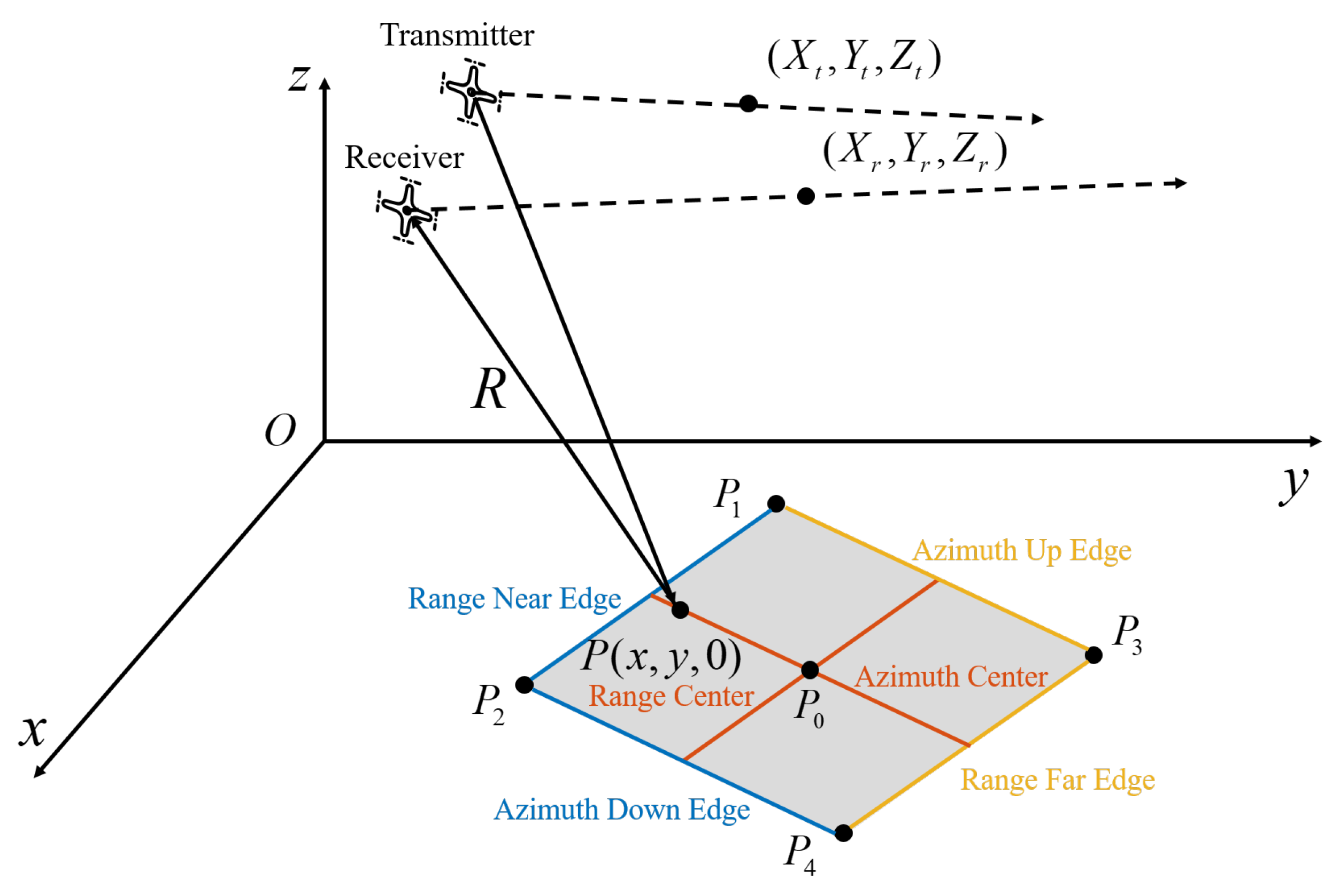
2.1. Slant Range Model

The transmitter and receiver both contribute to the slant range history of UAV Bi-SAR, which is the sum of radicals. Unlike the Mo-SAR, whose derivation of the signal spectrum is based on the single radical model, the form of the Bi-SAR slant range history model is complex double radicals, so it is difficult to use the phase of stationary principle (POSP) to solve the stationary phase point directly. Usually, Taylor expansion and series inversion [32] are combined to solve the stationary phase point and derive the spectrum of the Bi-SAR echo.
Consider an imaging scene of UAV Bi-SAR, as shown in Figure 1. P 1 , P 2 , which are distributed at the same range position, are close-range targets. Meanwhile, P 3 , P 4 are far-range targets, which are also distributed at the same range position. P 1 , P 3 are distributed at the same azimuth position, and so are P 2 , P 4 . P 0 represents the center point target of the scene, and P ( x , y , 0 ) represents any position’s target in the scene, whose slant history is expressed as
R ( t a ; x , y ) = X t + V t x t a x 2 + Y t + V t y t a y 2 + Z t + V t z t a 2 + X t + V t x t a x 2 + Y t + V t y t a y 2 + Z t + V t z t a 2
where X t , Y t , Z t is the coordinate position of transmitter at azimuth zero time, and X r , Y r , Z r is the one of the receivers. It can be obtained by sorting the Equation (1) according to the power of azimuth time as
R ( t a ; x , y ) = R t 0 2 + u t 1 t a + u t 2 t a 2 + R r 0 2 + u r 1 t a + u r 2 t a 2
where
R t 0 = X t x 2 + Y t y 2 + Z t z 2 u t 1 = 2 X t x V t x + 2 Y t y V t y + 2 Z t z V t z u t 2 = V t x 2 + V t y 2 + V t z 2 R r 0 = X r x 2 + Y r y 2 + Z r z 2 u t 1 = 2 X r x V r x + 2 Y r y V r y + 2 Z r z V r z u t 2 = V r x 2 + V r y 2 + V r z 2
It is difficult to solve the stationary phase point since the form of double radicals, so the Formula (2) can be expressed using Taylor expansion and kept in the fourth-order as follows:
R T a y l o r ( t a ; x , y ) = R b i s ( x , y ) + k 1 ( x , y ) t a + k 2 ( x , y ) t a 2 + k 3 ( x , y ) t a 3 + k 4 ( x , y ) t a 4
where
R b i s = R t 0 + R r 0 , f d c = k 1 λ k 1 = u t 1 2 R t + u r 1 2 R r k 2 = u t 2 2 R t + u r 2 2 R r u t 1 2 8 R t 3 u r 1 2 8 R r 3 k 3 = u t 1 u t 2 4 R t 3 u r 1 u r 2 4 R r 3 + u t 1 3 16 R t 5 + u r 1 3 16 R r 5 k 4 = u t 1 u t 2 4 R t 3 u r 1 u r 2 4 R r 3 + u t 1 3 16 R t 5 + u r 1 3 16 R r 5
The coefficients of the Taylor expansion have their own meanings. Specifically, R b i s represents the range position of the target after 2D focusing in RD plane, and the sum of all quantities in formula (4) except for R b i s means RCM. λ means the wave length of the RF signal. k 1 contains the information of range walking term and Doppler center f d c , that is, the azimuth position of target in RD plane. k 2 , k 3 and k 4 are collectively referred to as AFP, because they contain the information of azimuth non-linear phase, which cause large bandwidth in the Doppler domain. Also, they include the message of range curving and high-order RCM terms.
The difference between Formulas (2) and (4) is the slant range model error, which depends on the order of Taylor expansion. Generally, the higher order expansion we use, the higher accuracy we obtain. UAV Mo-SAR usually uses the second-order slant range model. However, the second-order slant range model cannot meet the imaging requirements of Bi-SAR. The slant range history errors corresponding to the second-order, third-order and fourth-order slant range models for scene edge points P 1 , P 2 , P 3 , P 4 and center point P 0 are shown in Figure 2.
It is generally agreed that the RCM error should not exceed half the range unit, and the phase error should not exceed pi/4. In the Ku band, the wavelength is 0.02 m and the range unit is 0.25 m in this article. Under the condition of precisely meeting the RCM error requirement, the phase error can reach approximately 40 radians, far exceeding the phase error requirement. Therefore, the phase error requirement is stricter than the RCM error requirement, and the model that meets the phase error requirement must meet the RCM error requirement. In the synthetic aperture time of 6 s, the maximum phase error caused by the second-order slant model is close to 62.8 radians, which is far from meeting the imaging requirements, and the phase error of the third-order model is about 2.5 radians, which is still not satisfy the requirement. While the phase error of the fourth-order model is less than 0.07 radians, which has sufficient precision. Therefore, in this paper, the slant range model is a fourth-order model.

2.2. UAV Bi-SAR Echo Model

The 2D time domain demodulated UAV Bi-SAR echo of target P ( x , y ) in spotlight mode is expressed as
s ( t a , t r ) = r e c t t r R t a ; x , y c T p r e c t t a T s × exp j π K r t r R t a ; x , y c 2 j 2 π λ R t a ; x , y
where t r and t a mean range time and azimuth time, T p and T s mean transmitting signal duration and sub-aperture duration, K r means range chirp rate, λ means the wavelength of radar system, c means the speed of light.
Then, we perform range-matching filtering on the echo, and approximate the slant range history to Taylor expansion model according to the discussion in Section 2.1. The result is as follows.
s ( t a , t r ) = s i n c t r R T a y l o r t a ; x , y c T p r e c t t a T s × exp j 2 π λ R T a y l o r t a ; x , y
where s i n c ( · ) and exp ( · ) represent the envelope and phase term of echo, respectively.

2.3. Spatial Variant AFP Model

Generally, in the SAR frequency domain imaging algorithm, the problem of spatial variation we discuss refers to the range-azimuth 2D spatial variation of RCM and ANP. In former analysis, we know that the spatial variation characteristics of AFP determine the spatial variation characteristics of RCM and ANP, that is, by modeling AFP, a unified spatial variation description of RCM and ANP can be achieved. The required model accuracy of AFP depends on the upper tolerance error limit of RCM and ANP.
Next, this article will analyze the 2D spatial variation modeling of AFP from the perspectives of RCM and ANP. In this article, we use NLCS to eliminate the variation of RCM and ANP. NLCS is a compensation method based on spatial variant AFP polynomial fitting models, so this method has errors whose size determines the quality of the imaging results. It is necessary to conduct error analysis on spatial variant AFP models, so as to design the most suitable spatial variant polynomial model for RCMC and ANPE.

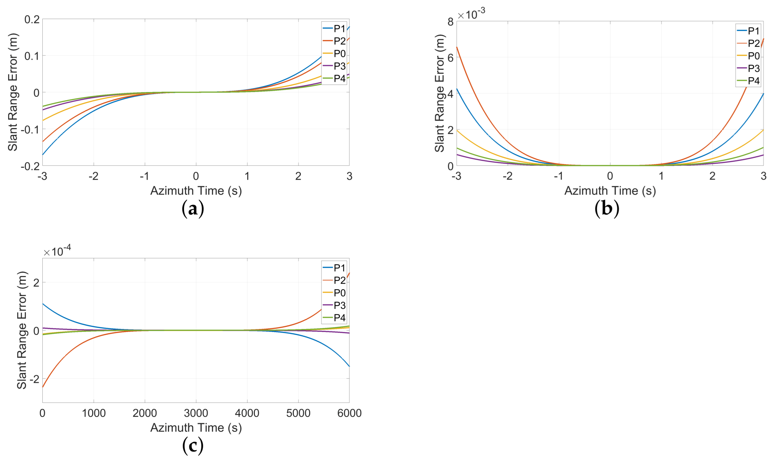
2.3.1. 2D Spatial Variant RCM

SAR imaging generally requires that the residual RCM after compensation should not exceed half of the range unit. According to Formulas (4) and (7), the RCM of the target P ( R b i s , f d c ) (he coordinates here are mapped from the ground plane to the range-Doppler plane) point can be expressed as
R r c m ( t a ; R b i s , f d c ) = k 1 ( f d c ) t a + k 2 ( R b i s , f d c ) t a 2 + k 3 ( R b i s , f d c ) t a 3 + k 4 ( R b i s , f d c ) t a 4
where the first term is the linear term of azimuth time t a , which is called the range-walking term; the second term is called the range-curving term; the third, fourth and other terms neglected in Formula (8) are referred to as the higher-order term of RCM.
The values of these terms change with R b i s , f d c , and we call it the 2D spatial variation of RCM. The value scaling of azimuth time t a is T s / 2 , T s / 2 . According to Formula (8), the spatial variation of RCM will be more serious with the increase of synthetic aperture time. As long as the maximum residual RCM corresponding to t a = ± T s / 2 is not more than half of the resolution unit, the spatial variant model is considered to meet the demand. In this paper, the spatial variation of RCM in 6 s synthetic aperture time is investigated.
Due to the use of RNCS, we should consider the order of AFP polynomial fitting along range direction, and the details about RNCS will be introduced later. Here, we use least squares (LS) method to estimate the coefficients of each order term of polynomial fitting. Distinguished with ANCS, because RCM of each order term is independent with range time t r , the AFP of each order can be fitted in the same order, that is
k 2 = k 20 r + k 21 r R b i s R b i s , c + k 22 r R b i s R b i s , c 2 k 3 = k 30 r + k 31 r R b i s R b i s , c + k 32 r R b i s R b i s , c 2 k 4 = k 40 r + k 41 r R b i s R b i s , c + k 42 r R b i s R b i s , c 2
where k i j r means the j t h order coefficient of i t h order of AFP, and R b i s , c means the reference range of whole scene. Then, we convert the AFP spatial variant model error to maximum RCM error.
First-order and second-order fitting of AFP along the range direction are considered here, and the corresponding fitting error results are shown in Figure 3. The maximum error of the first-order fitting is 0.3 m, while the second-order fitting is only about 0.05 m. Therefore, under the requirements of 0.25 m resolution imaging in this paper, second-order fitting is adequate. That is to say, the accuracy of the range spatial variant AFP model applied to RCNS is sufficient.

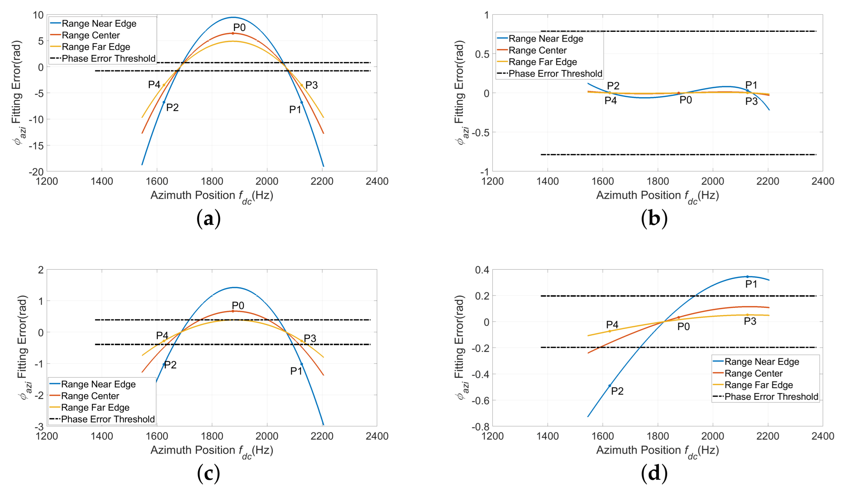
2.3.2. 2D Spatial Variant ANP

SAR imaging generally requires that the quadratic residual phase after azimuth focusing should not exceed π / 4 , the cubic residual phase should not exceed π / 8 , the quartic phase should not exceed π / 16 . According to Formulas (4) and (7), and ignoring linear and constant phase terms, the azimuth phase of target P ( R b i s , f d c , 0 ) can be expressed as
ϕ a z i ( t a ; R b i s , f d c ) = 2 π λ k 2 ( R b i s , f d c ) t a 2 2 π λ k 3 ( R b i s , f d c ) t a 3 2 π λ k 4 ( R b i s , f d c ) t a 4
where λ is the wavelength of the carrier, the quadratic term of t a corresponding to k 2 ( R b i s , f d c ) is called the quadratic phase, the cubic term of t a corresponding to k 3 ( R b i s , f d c ) is called the cubic phase and the quartic term of t a corresponding to k 4 ( R b i s , f d c ) is called the quartic phase.
In this paper, we use Ku band for high-resolution SAR imaging. It can be seen from Formulas (8) and (10) that the residual RCM will be magnified by hundreds of times on the phase because of the short wavelength. The spatial variation of the azimuth phase in a 6 s synthetic aperture time is investigated. Since the azimuth linear phase spatial variation contains the azimuth position information, it does not need compensation and removal. Here, only the quadratic, cubic and quartic phase spatial variations are discussed. According to the discussion in Section 2.3.1, as long as the corresponding maximum quadratic, cubic and quartic phase compensation error does not exceed π / 4 , π / 8 and π / 16 respectively, the spatial variant model is considered to meet the imaging requirements.
Similarly, we can model as follows.
k 2 = k 20 a + k 21 a f d c f d c , c + k 22 a f d c f d c , c 2 k 3 = k 30 a + k 31 a f d c f d c , c k 4 = k 40 a
where k i j a means the j t h order coefficient of i t h order of AFP in azimuth direction, and f d c , c means the azimuth position of the reference target in whole scene. Then, we convert the AFP spatial variant model error to maximum ANP error.
Also, because of the ANCS, like the consideration of RNCS, we should analyse the fitting polynomial of k 2 , k 3 and k 4 . The polynomial fitting of the quadratic phase is carried out in Figure 4, and the fitting error is up to 7 radians, exceeding π / 4 , while the second-order fitting error is not more than 0.025 radians. The first-order fitting maximum error of the cubic phase is about 1 radian, exceeding π / 8 . The zero-order fitting maximum error of quartic phase is about 0.5 radians, exceeding π / 16 . Therefore, under the requirements of SAR imaging, although we perform second-order fitting on the quadratic phase, first-order fitting on the cubic phase and zero-order fitting on the quartic phase, the accuracy of the azimuth spatial variant AFP is not enough. That is, the accuracy of ANCS will be challenged. So, we will introduce Doppler blocking to solve this problem in the following text.

3. Imaging Algorithm

A traditional frequency domain imaging algorithm for spotlight SAR is mainly divided into three steps: range compression, RCMC and azimuth deramp. In this article, on this basis, we propose an imaging algorithm based on Doppler blocking and 2D NLCS to eliminate the spatial variation of RCM and ANP effectively. And this method can adapt to severe azimuth spatial variation environment for UAV Bi-SAR while traditional methods and some contrast methods like [30,31] cannot. Specifically, we divide RCMC into two parts: RWC and residual RCMC. First, we compensate the bulk term of RCM and second range compression (SRC). Second, we use keystone transform to perform 2D spatial variant RWC. Third, Doppler blocking is carried on, and 2D NLCS is performed in Doppler blocks purposely to achieve two keys. The first key is to reduce azimuth spatial variation of residual RCM so that it can be neglected. And the second key is reducing the spatial variation model error of ANCS to meet the imaging requirements and solve image distortion and false targets problems caused by traditional ANCS by the way. In order to distinguish from traditional ANCS, we call this method frequency division ANCS. Then, in Doppler blocks, we use RNCS to eliminate range spatial variation of RCM as much as possible and use ANCS to remove azimuth spatial variation of ANP. Finally, azimuth deramp is performed to obtain a well-focused image.

3.1. RWC Based on Keystone Transform

Many articles have elaborated on the principle and processing of keystone transform to remove the range walking of 2D spatial variation, and this operation is not the innovation of this paper. So, we will briefly explain the principle and directly give processed results. Keystone transform is widely used because it can provide nonparametric RWC. Its essence is to scale azimuth time axis in range frequency domain to eliminate the coupling between range frequency and azimuth time, namely, keep azimuth time axis unchanged at the zero point of range frequency, stretch it where range frequency is positive, and shrink it where range frequency is negative.
The result of range Fourier transform and the bulk RWC of the demodulated echo signal is as follows
s ( t a , f r ) = r e c t f r K r T p r e c t t a T s × exp j π f r 2 K r j 2 π f c + f r c R b i s + k 1 k 1 r e f t a + k 2 t a 2 + k 3 t a 3 + k 4 t a 4
where f c and f r represent carrier frequency and range frequency, respectively. k 1 r e f means the first order coefficient of Taylor expansion of scene center reference target’s range history. K r means range chirp rate, and T p represents range signal duration. Keystone transform can be expressed as
t a = f c f c + f r t m
Substitute Formula (13) into Formula (12), and then perform Taylor expansion at the range frequency zero point, that is
s r w c ( t a , f r ) = r e c t f r K r T p r e c t t a T s f c f c + f r × exp { j π f r 2 K r j 2 π c R b i s f r j 2 π λ R b i s + k 1 t a + k 2 t a 2 + k 3 t a 3 + k 4 t a 4 j 2 π c k 2 t a 2 2 k 3 t a 3 3 k 4 t a 4 f r j 2 π f c c k 2 t a 2 + 3 k 3 t a 3 f r 2 }
It can be seen from Formula (14) that the third term (azimuth phase term) does not change after keystone transform, which is convenient for us to perform azimuth deramp. However, the residual RCM term has changed; in particular the coefficient of k 3 and k 4 have changed to not 1. And the spatial variation of fifth term (SRC term) can be ignored, so only the spatial variation of RCM needs to be considered. This shows that keystone transform can provide nonparametric RWC without changing the azimuth phase.

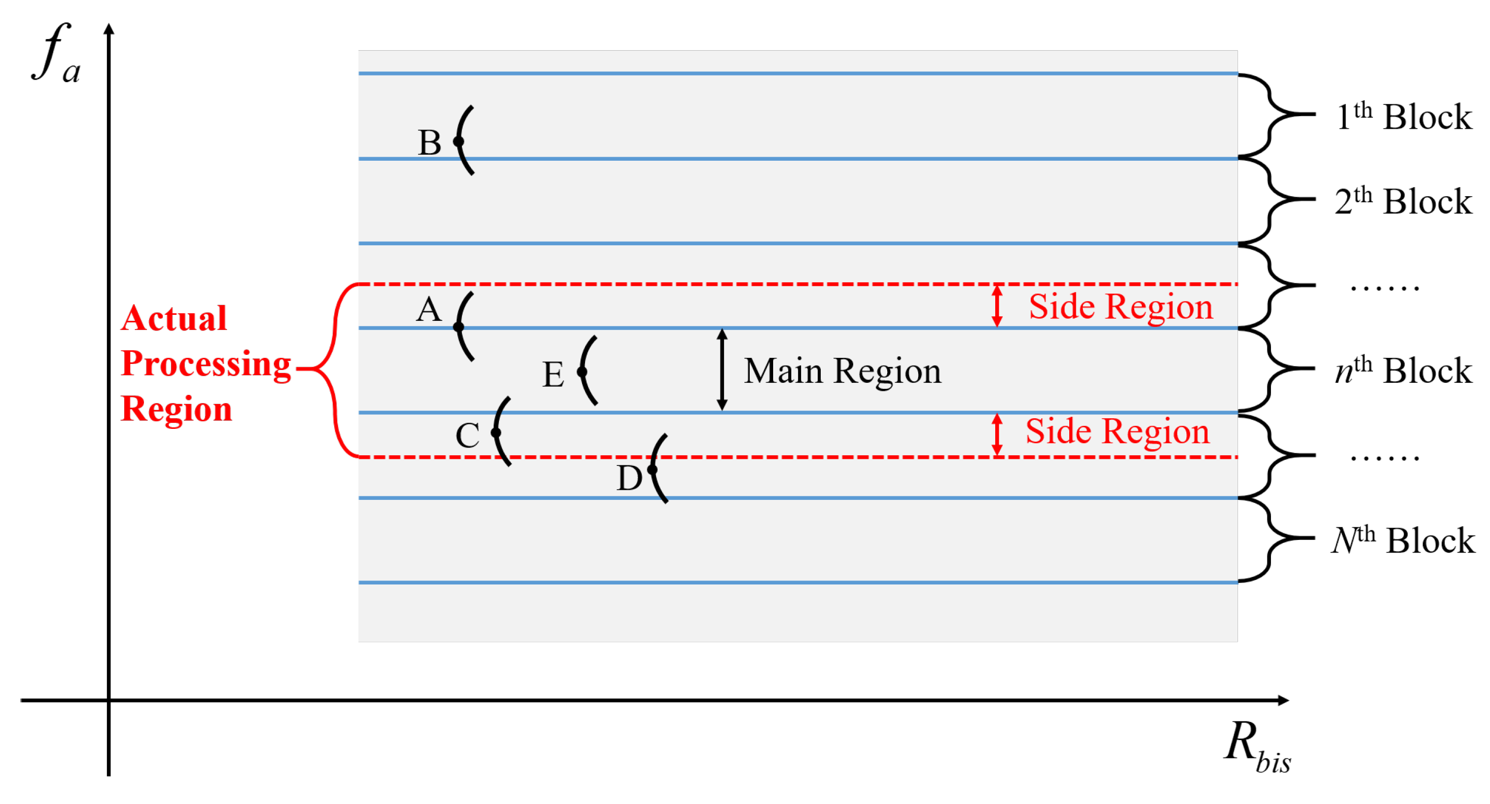
3.2. Azimuth Spatial Variant Residual RCMC Based on Doppler Blocking

The existing methods struggle to solve the 2D spatial variant problem of RCM. Thanks to the NLCS algorithm, we can use it to complete the range spatial variant RCMC. For the azimuth spatial variance, we proposed the method of azimuth spatial variant RCMC based on Doppler blocking.
This section will introduce the Doppler blocking operation. The echo after RWC is divided into several blocks, which reduces the scale of each block processing in Doppler domain, so as to reduce the azimuth spatial variation of RCM to be negligible, and then RCM of targets in the same block can be uniformly corrected. Doppler blocking can approximately distinguish the support domains of different targets based on the characteristics that targets in different azimuth positions have, such as different Doppler centers in spotlight mode. Taking a certain block as an example, since the blocking operation is carried out before azimuth deramp, the energy of targets will be dispersed to different Doppler units, so only part of the targets’ total energy will fall into the sub-block (i.e., the main region), like point E as shown in Figure 5. A large amount of targets fall incompletely in the main region, such as point A, B, C and D. In order to avoid these incomplete accumulation points, overlapping areas are added between blocks, which are called side regions compared with the main region, and each main region has two side regions above and below it. The size of side regions is set to half of the maximum Doppler bandwidth of all targets in the scene to ensure that all targets falling into the main region are complete accumulation points. The Doppler center of target A is located at the edge of the main region in the n t h block, and only half of its energy falls in the main area. Due to the side regions, its energy will all fall into the n t h block after the azimuth deramp. However, side regions will introduce the energy of targets whose azimuth positions are outside the main area, such as point C and D. But after azimuth focusing, the focused targets fall into the side region, so it is convenient to remove these side region points, just retaining the main area. Thereby, one main region and its adjacent two side regions are added together, which we call the actual processing region. Our algorithm works one-by-one with these actual processing regions, and finally discards the side regions, retains the main regions and splices the main regions together.
Next, we introduce the principle of removing the intra-region azimuth spatial variant residual RCM. First, the Doppler center of any point target in the scene must fall within a main region or on its edge. In Figure 6a, point A is located in the side region and point B is located in the main region. The whole energy of both targets is included in the actual processing region. Then, the residual RCMC is performed in the azimuth time domain as shown in Figure 6b. We assume the use of the AFP of the azimuth reference point will be at a certain range in the main region for RCMC (in fact, we will not perform the azimuth bulk RCMC in this way, as the bulk term will be compensated by range bulk RCMC and range spatial variant RCMC, and this assumption is only made for the convenience of illustration), then if the point target falls in the main region or on its edge, like point B, under the condition of reasonable Doppler blocking, it should meet the condition that the residual RCM can be ignored, compared as shown in Figure 6c. Under current assumptions, specifically, the residual RCM of targets can be expressed as
Δ r e s R C M = k 2 k 20 a t a 2 + 2 k 3 k 30 a t a 3 + 3 k 4 k 40 a t a 4 = Δ k 2 a t a 2 + 2 Δ k 3 a t a 3 + 3 Δ k 4 a t a 4
where k 2 , k 3 and k 4 mean the AFP of targets, k 20 a , k 30 a and k 40 a mean the AFP at the azimuth reference frequency f d c , c and a certain slant range R b i s and Δ k 2 a , Δ k 3 a and Δ k 4 a represent the azimuth spatial variation of AFP. As shown in Figure 6c, Δ r e s R C M A and Δ r e s R C M B mean the residual RCM of target A and B, respectively, after assumed azimuth bulk RCMC.
If the point target falls in the side region, like point A, the residual RCM cannot be ignored at this time as shown in Figure 6c,d, and it is just discarded due to falling in the side region after azimuth deramp. Therefore, the residual RCM after assumed azimuth bulk RCMC for all targets in the main region should not exceed the tolerable upper limit (the azimuth variations in different range units are different, and the azimuth residual RCM of all targets in all different range units should meet this condition). Usually, the upper limit is set to half of the range unit.
In summary, the first advantage of Doppler blocking is to solve the problem of azimuth spatial variation of RCM, so it is necessary to ensure that the azimuth spatial variation of RCM within every block can be ignored, that is, to meet the
Δ k 2 a , n T a 2 2 + 2 Δ k 3 a , n T a 2 3 + 3 Δ k 4 a , n T a 2 4 c 2 f s , n = 1 , 2 , , N
where Δ k 2 a , n , Δ k 3 a , n and Δ k 4 a , n means azimuth spatial variant components of k 2 , k 3 and k 4 relative to azimuth reference targets in all range units in the n t h block, T a means synthetic aperture time and f s means range sampling rate. N represents the number of Doppler blocks.
As we all know, the azimuth spatial variations of RCM between near and far range points are quite different. Further speaking, azimuth spatial variation of near range points is more serious. In order to ensure that the azimuth spatial variation of RCM within every block can be ignored, for convenient, only Δ k 2 a , n , Δ k 3 a , n and Δ k 4 a , n of near range targets should be considered in Formula (16). This ensures that Δ k 2 a , n , Δ k 3 a , n and Δ k 4 a , n of all targets in the scene meet Formula (16).

3.3. Range Spatial Variant Residual RCMC Based on RNCS

After Doppler blocking, the azimuth spatial variation of RCM within the block can be ignored, but the range spatial variation cannot be ignored. We use RNCS to remove the range spatial variation term of RCM. The following is a brief description of the RNCS operation in spotlight mode.
First, polynomial fitting is carried out at the reference point along the range direction for the spatial variant AFP in a block:
k 2 = k 20 r + k 21 r ( R b i s R b i s , c ) + k 22 r ( R b i s R b i s , c ) 2 k 3 = k 30 r + k 31 r ( R b i s R b i s , c ) + k 32 r ( R b i s R b i s , c ) 2 k 4 = k 40 r + k 41 r ( R b i s R b i s , c ) + k 42 r ( R b i s R b i s , c ) 2
where k 20 r , k 30 r and k 40 r mean the bulk term and also mean the value of k 2 , k 3 and k 4 at the reference point, respectively. k 21 r , k 31 r , k 41 r and k 22 r , k 32 r , k 42 r represent the coefficients of the linear and quadratic terms of the expansion. R b i s , c means the range position of the reference point.
Since the NLCS operation introduces additional range frequency linear term, quadratic term and additional azimuth phase, in order to eliminate the range spatial variation of RCM without introducing additional range frequency correlation term, it is necessary to introduce an additional cubic term to compensate the correlation term introduced by RNCS.
For the signal after keystone transform and Doppler blocking, we perform range Fourier transform firstly and then multiply the compensation phase by the following:
H r p = exp j π 2 3 Y r f r 3
where the additional cubic compensational factor Y r will be given in following text.
Then, we perform inverse Fourier transform in the range direction without considering the azimuth phase term, and the signal expression is as follows.
s r w c 1 ( t r , t a , s u b ) = r e c t t r R n / c T p r e c t t a , s u b T s × exp j π K r t r R n c 2 + j π 2 3 Y r K r 3 t r R n c 3
where R n means the RCM curve of targets after RWC, and its specific expression is given by
R n = R b i s k 2 t a , s u b 2 2 k 3 t a , s u b 3 3 k 4 t a , s u b 4
Secondly, we multiply the disturbance phase and the signal in Formula (19) in the range time domain, and the phase is given by
H r n c s = exp j π q 2 r t r R n , c c 2 + j π 2 3 q 3 r t r R n , c c 3
where R n , c represents the RCM curve of the range reference target after RWC, and its specific expression is like Formula (20) only if R b i s is substituted by R b i s , c and k 2 , k 3 and k 4 is replaced by k 20 r , k 30 r and k 40 r .
Based on the fact that the RCM spatial variation and the additional range frequency correlation be zero after perturbation, the coefficients of the perturbation phase and the additional cubic phase can be solved, which are given by
q 2 r = K r ( k 21 r t a 2 + 2 k 31 r t a 3 + 3 k 41 r t a 4 ) q 3 r c K r ( k 22 r t a 2 + 2 k 32 r t a 3 + k 42 r t a 4 ) Y r = q 3 r / ( q 2 r K r 2 )
After RNCS, the matched filter also needs to be adjusted accordingly, that is
H f = exp j π 2 3 Y r K r 3 + q 3 r K r + q 2 r 3 f r 3 + j π 1 K r + q 2 r f r 2
At the same time, the azimuth phase introduced by RNCS needs to be compensated before the azimuth phase processing. This step is completed in the azimuth time domain, that is, multiplied by
H r e s = exp j π K r q 2 r K r + q 2 r R n R n , c c 2 j π 2 q 3 r K r 3 Y r K r 3 q 2 r 3 3 K r + q 2 r 3 R n R n , c c 3

3.4. Azimuth Spatial Variant ANPE Based on ANCS Combined with Doppler Blocking

After RCMC, only the ANP needs to be considered. ANCS makes use of the characteristics of different support areas in Doppler domain of different targets, and compensates for the corresponding phases of different positions in the Doppler domain, so that all targets within the same range unit have the same AFP, which will be used to construct a unified deramp function. The following will introduce the process of ANCS combined with Doppler blocking in detail.
The signal after Doppler blocking and RCMC can be expressed as
s r c m c ( t r , t a , s u b ) = sin c t r R b i s c r e c t t a , s u b T a × exp j 2 π f d c , s u b t a , s u b j 2 π R b i s λ × exp j 2 π λ k 2 t a , s u b 2 k 3 t a , s u b 3 k 4 t a , s u b 4
where t a , s u b means the azimuth time in sub-blocks. In fact, the support area of t a , s u b is the same as t a . And f d c , s u b means the azimuth position of targets in sub-blocks, which is determined by the azimuth positions of targets before Doppler blocking and the center positions of sub-blocks.
First, we multiply the signal by the compensation phase, whose role is consistent with the compensation phase in Formula (18) of the above RNCS, and its expression is
H a p = exp j 2 π Y a λ t a , s u b 3
where the calculation method of Y a will be mentioned later.
Then, we carry out azimuth Fourier transform, and the processed signal in Doppler domain is expressed as
s r c m c 1 ( t r , f a , s u b ) = s i n c t r R b i s c r e c t f a , s u b f d c , s u b B a × exp j 2 π R b i s λ × exp j 2 π u 2 f a , s u b f d c , s u b 2 + u 3 f a , s u b f d c , s u b 3 + u 4 f a , s u b f d c , s u b 4
where f a , s u b means the azimuth frequency of sub-blocks, and its support area becomes shorter because of Doppler blocking. According to POSP and series reversion, the coefficients of quadratic, cubic and quartic phase in the Doppler domain can be determined by the following expression.
u 2 = λ 1 4 k 2 u 3 = λ 2 k 3 + Y a 8 k 2 3 u 4 = λ 3 4 k 4 k 2 + 9 k 3 + Y a 2 64 k 2 5
The polynomial fitting of u 2 , u 3 and u 4 along the azimuth direction is as follows:
u 2 = u 20 a + u 21 a f d c , s u b + u 22 a f d c , s u b 2 u 3 = u 30 a + u 31 a f d c , s u b u 4 = u 40 a
Next, the disturbance phase is multiplied in Doppler domain,
H a n c s = exp j 2 π q 3 a f a , s u b 3 + j 2 π q 4 a f a , s u b 4
where q 3 a , q 4 a represent the coefficients of disturbance phase.
According to the fact that the spatial variant ANP with the factor f d c , s u b be zero after perturbation, we can solve the coefficients of perturbation phase and addition cubic phase. Note that the function of Y a is to balance the equation: 4 q 4 a + u 31 a = 0 .
q 3 a = u 21 a 3 q 4 a = u 22 a 6 Y a = q 4 a + 2 u 20 a 3 k 31 a 6 u 20 a 2 u 21 a k 30 a
where
k 30 a = k 3 ( R b i s , f d c , s u b ) f d c , s u b = 0 k 31 a = d k 3 ( R b i s , f d c , s u b ) d f d c , s u b f d c , s u b = 0
After completing ANCS, the difference of targets’ AFP at different azimuth positions is eliminated, and the unified azimuth reference function can be used for azimuth compression. Since the ANCS introduces addtional cubic and quartic phases, the azimuth reference function is modified as follows.
H a = exp j 2 π λ k 20 a t a , s u b 2 + j 2 π λ k 30 a + 8 k 20 a 3 q 3 a λ 2 + Y a t a , s u b 3 + j 2 π λ k 40 a + 36 k 20 a 2 k 30 a + Y a q 3 a λ 2 16 k 20 a 4 q 4 a λ 3 + 144 k 20 a 5 q 3 a 2 λ 4 t a , s u b 4
where
k 20 a = k 2 ( R b i s , f d c , s u b ) f d c , s u b = 0 k 30 a = k 3 ( R b i s , f d c , s u b ) f d c , s u b = 0 k 40 a = k 4 ( R b i s , f d c , s u b ) f d c , s u b = 0
It is precisely because there are fitting errors in Formula (29), that is, there is accuracy issue with the azimuth spatial variance AFP model, that we need to apply Doppler blocking to solve it. And the upper limit of the tolerable error within the block will determine the lower limit of the number of blocks. We will analyze the impact of fitting errors within the sub-blocks on the azimuth deramp and provide the second criterion for Doppler blocking.
First, we rewrite the Formula (29) to the form with errors as
u 2 = u 20 a + u 21 a f d c , s u b + u 22 a f d c , s u b 2 + δ 1 ( f d c , s u b ) u 3 = u 30 a + u 31 a f d c , s u b + δ 2 ( f d c , s u b ) u 4 = u 40 a + δ 3 ( f d c , s u b )
where δ 1 ( f d c , s u b ) , δ 2 ( f d c , s u b ) and δ 3 ( f d c , s u b ) mean the polynomial fitting error of Doppler AFP u 2 , u 3 and u 4 for the target at a certain azimuth position f d c , s u b .
Combining Formulas (27), (29) and (31), we find that ANCS can accurately eliminate the first-order and second-order fitting coefficients of the quadratic phase u 21 a , u 22 a , but the first-order fitting coefficient of the cubic phase u 31 a is eliminated by Y a balancing equation, which will not be valid in the presence of model errors. Therefore, the first-order fitting coefficient of the cubic phase cannot be completely eliminated. Specifically, neglecting the signal envelope term and constant phase term, only focusing on the non-constant phase term, the phase of signal after ANCS in the case of existing errors is expressed as,
ϕ a n c s ( f a , s u b ) = exp j 2 π 4 q 4 a f d c , s u b 3 + 3 q 3 a f d c , s u b 2 f a , s u b f d c , s u b + u 20 a + δ 1 ( f d c , s u b ) f a , s u b f d c , s u b 2 + u 30 a + q 3 a + δ 2 ( f d c , s u b ) + 4 q 4 a f d c , s u b + u 31 a f d c , s u b f a , s u b f d c , s u b 3 + u 40 a + q 4 a + δ 3 ( f d c , s u b ) f a , s u b f d c , s u b 4
where the first term in the Formula (36) is the spatial variant linear phase introduced by ANCS, which can be eliminated in subsequent distortion correction (under appropriate Doppler blocking, this linear phase will be very small, thus eliminating the need for distortion correction in proposed algorithm); the second and fourth error terms are both introduced by the lack of azimuth spatial variant AFP model accuracy; the third error term is introduced by equation imbalance and lack of model accuracy.
Thus, the AFP errors in Doppler domain after ANCS can be obtained, as shown in Formula (37).
Δ u 2 a , n = δ 1 ( f d c , s u b ) Δ u 3 a , n = δ 2 ( f d c , s u b ) + 4 q 4 a + u 31 a f d c , s u b Δ u 4 a , n = δ 3 ( f d c , s u b )
where Δ u 2 a , n , Δ u 3 a , n and Δ u 4 a , n means the errors of spatial invariant AFP after ANCS and in n t h Doppler block.
Due to the time domain deramp imaging, we also need to convert the AFP errors in Doppler domain Δ u 2 a , n , Δ u 3 a , n , Δ u 4 a , n to time domain based on POSP. So, we transform the signal in Formula (36) into the azimuth time domain, and its expression is as follows.
ϕ a n c s ( t a , s u b ) = exp j 2 π f d c , s u b t a , s u b + Δ t a , s u b + k ^ 2 a , n + Δ k ^ 2 a , n t a , s u b + Δ t a , s u b 2 + k ^ 3 a , n + Δ k ^ 3 a , n t a , s u b + Δ t a , s u b 3 + k ^ 4 a , n + Δ k ^ 4 a , n t a , s u b + Δ t a , s u b 4
where Δ t a , s u b means the offset of time domain support area introduced by ANCS in Formula (36), that is Δ t a , s u b = 4 q 4 a f d c , s u b 3 + 3 q 3 a f d c , s u b 2 , and k ^ 2 a , n , k ^ 3 a , n and k ^ 4 a , n mean the time domain deramping function coefficients obtained from Doppler domain inverse calculation without considering spatial variant AFP model fitting errors. Δ k ^ 2 a , n , Δ k ^ 3 a , n and Δ k ^ 4 a , n mean the AFP errors before azimuth deramping (the superscript hat is used to distinguish them from the coefficients in Formula (16), unlike these coefficients, the ones with superscript hat represent the coefficients calculated through POSP inverse from the Doppler domain AFP errors Δ u 2 a , n , Δ u 3 a , n and Δ u 4 a , n ), as shown in Formula (37).
The azimuth deramping function is shown in Formula (33), and we find that due to the offset of signal support area Δ t a , s u b , the constructed uniform deramping function introduces new phase errors, specifically as shown in Formula (39).
Δ ϕ ( t a , s u b ) = exp { j 2 π f d c , s u b + 2 Δ t a , s u b k ^ 2 a , n + Δ k ^ 2 a , n + 3 Δ t a , s u b 2 k ^ 3 a , n + Δ k ^ 3 a , n + 4 Δ t a , s u b 3 k ^ 4 a , n + Δ k ^ 4 a , n t a , s u b Δ k ^ 2 a , n + 3 Δ t a , s u b k ^ 3 a , n + Δ k ^ 3 a , n + 6 Δ t a , s u b 2 k ^ 4 a , n + Δ k ^ 4 a , n t a , s u b 2 + Δ k ^ 3 a , n + 4 Δ t a , s u b k ^ 4 a , n + Δ k ^ 4 a , n t a , s u b 3 + Δ k ^ 4 a , n t a , s u b 4 }
So, according to the discussion in Section 2.3.2 we can provide the second Doppler blocking criterion, which can be expressed as
2 π λ Δ k ^ 2 a , n + 3 Δ t a , s u b k ^ 3 a , n + Δ k ^ 3 a , n + 6 Δ t a , s u b 2 k ^ 4 a , n + Δ k ^ 4 a , n T a 2 2 π 4 2 π λ Δ k ^ 3 a , n + 4 Δ t a , s u b k ^ 4 a , n + Δ k ^ 4 a , n T a 2 3 π 8 2 π λ Δ k ^ 4 a , n T a 2 4 π 16 , n = 1 , 2 , , N
Additionally, to avoid distortion correction, we require that the azimuth position distortion of targets caused by the support area offset introduced by ANCS should not exceed half of the azimuth unit, which is the third criterion for Doppler blocking.
2 Δ t a , s u b k ^ 2 a , n + Δ k ^ 2 a , n + 3 Δ t a , s u b 2 k ^ 3 a , n + Δ k ^ 3 a , n + 4 Δ t a , s u b 3 k ^ 4 a , n + Δ k ^ 4 a , n P R F 2 N a
The number of Doppler blocks depends on the three criteria mentioned in Formulas (16), (40) and (41). The minimum number of blocks N m i n that meet these three criteria is the appropriate numbers of Doppler blocks. The intra-block azimuth spatial variant RCM under this condition, the intra block azimuth spatial variant AFP model errors, the support area movement in time domain caused by ANCS (i.e., the azimuth position distortion in Doppler domain) and the ANP errors caused by the support area movement can be ignored.
Finally, the SAR image can be obtained by azimuth Fourier transform. The whole process of the imaging algorithm is shown in Figure 7. In actual scene SAR imaging, motion compensation is required before imaging, but motion compensation is not the key of this article. So, we use preprocessed data to describe the raw data after motion compensation.

4. Simulation and Verification
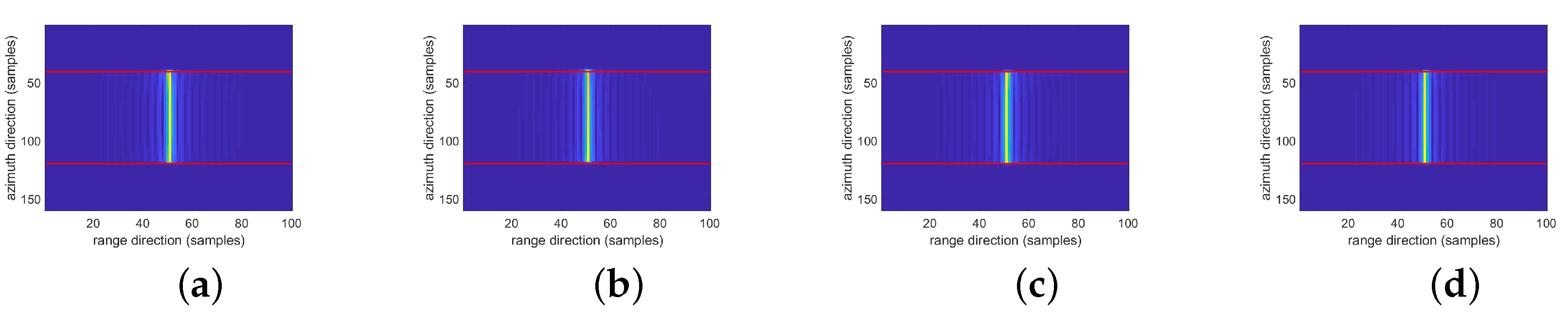
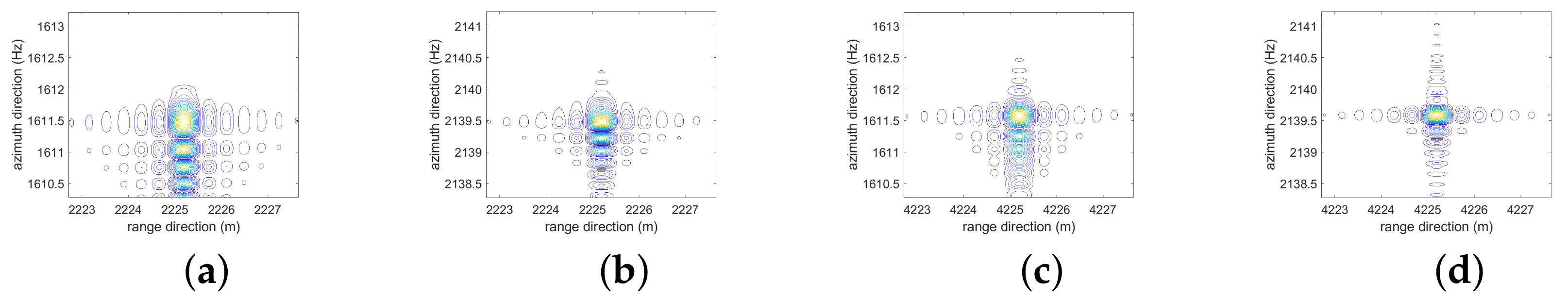
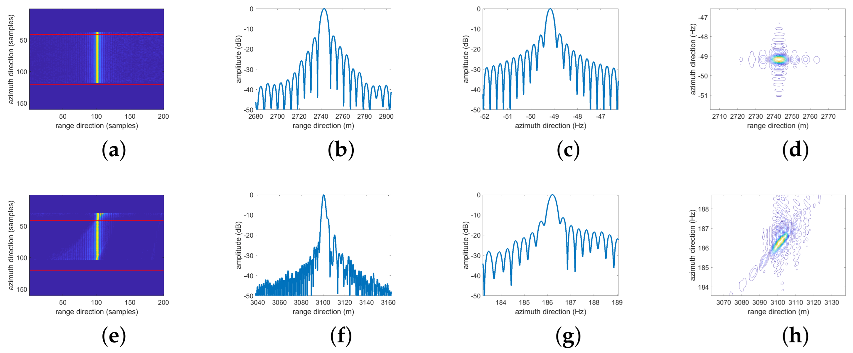
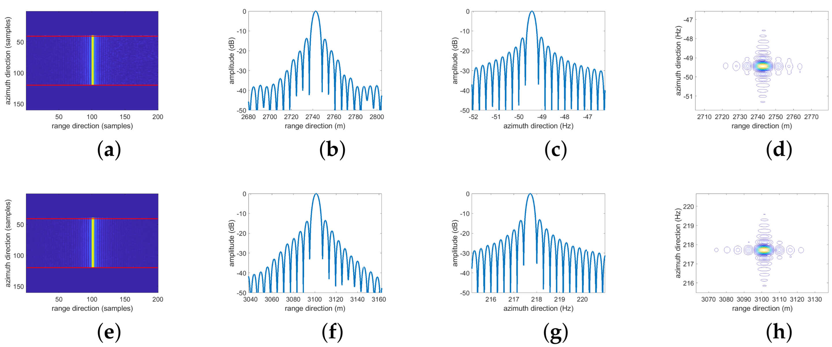
4.1. Simulation

The Bi-SAR echo data of targets array is simulated and processed to verify the effectiveness of the proposed algorithm. To verify the progressiveness of the proposed algorithm, we choose an algorithm [31] proposed in the published literature to compare the imaging performance. In echo simulation, the carrier frequency is 15 GHz, the bandwidth of the transmitted chirp is 800 MHz, and the sub-aperture duration is 6 s. The geometry of Bi-SAR and imaging scene is shown in Figure 8a. The transmitter and receiver fly along the y-axis at different speeds, and Bi-SAR works in shift-variant configuration and squint spotlight imaging mode. The size of imaging scene is 1000 m × 400 m as shown in Figure 8b (for the convenience of describing the scene width, the distribution of targets in Figure 8 is approximated as a rectangle, which is not the case in reality). There are nine targets in the simulated echo, with equal range and Doppler interval distribution in the range–Doppler plane. We only observe five of them, namely the scene center point P 0 and four range-azimuth edge points P 1 , P 2 , P 3 and P 4 . The center target of scene P 0 is at (2000, 500, 0) m. Specific simulation system parameters are shown in Table 1.
Figure 9 is the final processed image of the 3 × 3 points array with the proposed algorithm. We perform 16x upsampling on the 4 edge points of the whole scene, and their contour maps are shown in Figure 10 and Figure 11. There are two groups of up-sampling azimuth slice of point targets in Figure 12. The images in Figure 11 are processed according to the algorithm in [31], and these targets are defocused mainly in azimuth directions, which is caused by the residual azimuth spatial variant RCM and AFP. The images processed by the proposed algorithm are focused well, as shown in Figure 10. Table 2 shows the imaging evaluation results of the four edge points, which are in good agreement with the theoretical values, where the theoretical range and azimuth resolution values are 0.166125 m and 0.147667 Hz and the theoretical PSLR and ISLR values are −13.26 dB and −10.20 dB, respectively. The simulation results are reasonable, indicating that the imaging algorithm is effective.
To analyse the effect of Doppler blocking on azimuth spatial RCMC, the differences between the residual RCM of targets in different azimuth position after RCMC with Doppler blocking and without it are given in Figure 13 and Figure 14. In Figure 13, we find that the azimuth spatial variant range curving and RCM high-order terms are not compensated, which will seriously affect the target focusing. While in Figure 14, we know that with Doppler blocking, the residual RCM is not more than half a range unit length, that is, residual RCM is too small to be ignored. The area between the two red lines is the original time domain support area, and the area outside the red line is the newly support area after zeros-padding. The shift of support area in Figure 13 is due to linear phase introduced by ANCS. Due to significant movement of the support area in the time domain, false targets may occur in existing method. To eliminate this problem, the zeros-padding operation is required, which will also increase computational complexity. However, the proposed algorithm does not require zeros-padding as shown in Figure 14 (The zeros-padding in Figure 14 is for the convenience of observing the movement of its support domain, and there is no zeros-padding step in the actual proposed algorithm). That is to say, the proposed method only needs to perform Doppler blocking to solve the above pain points.
Considering the other advantage of Doppler blocking, we the simulate echo and process it with the RCMC part of the proposed method and the AFPE part of the existing method. The results are shown in Figure 15. From Figure 15, we find out that when the azimuth width is large, without Doppler blocking, the fitting errors of spatial variant AFP model will be significant, meaning that ANCS cannot completely eliminate them. Comparing this with Figure 10, with Doppler blocking, the spatial variant width of AFP in Doppler blocks is smaller, that is, the spatial variation of AFP is small enough, so the accuracy of spatial variant AFP model is high enough and ANCS can fully achieve its original purpose. The significant azimuth defocusing in the Figure 15 can prove this, while in Figure 10, the targets are well focused.

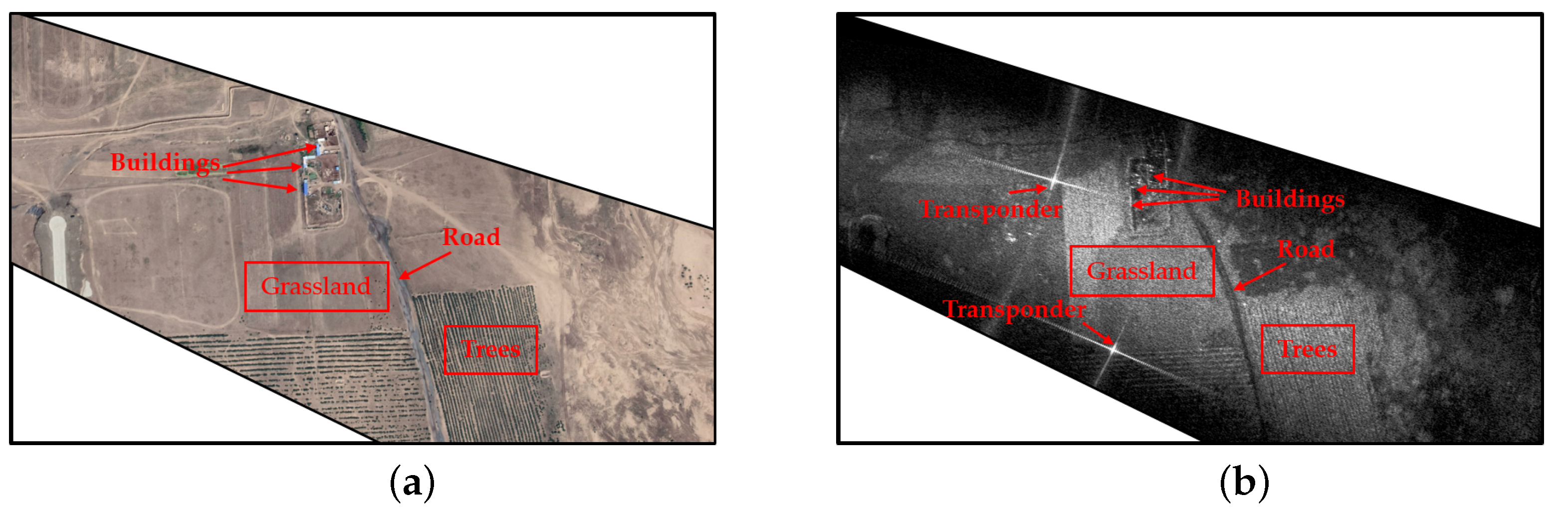
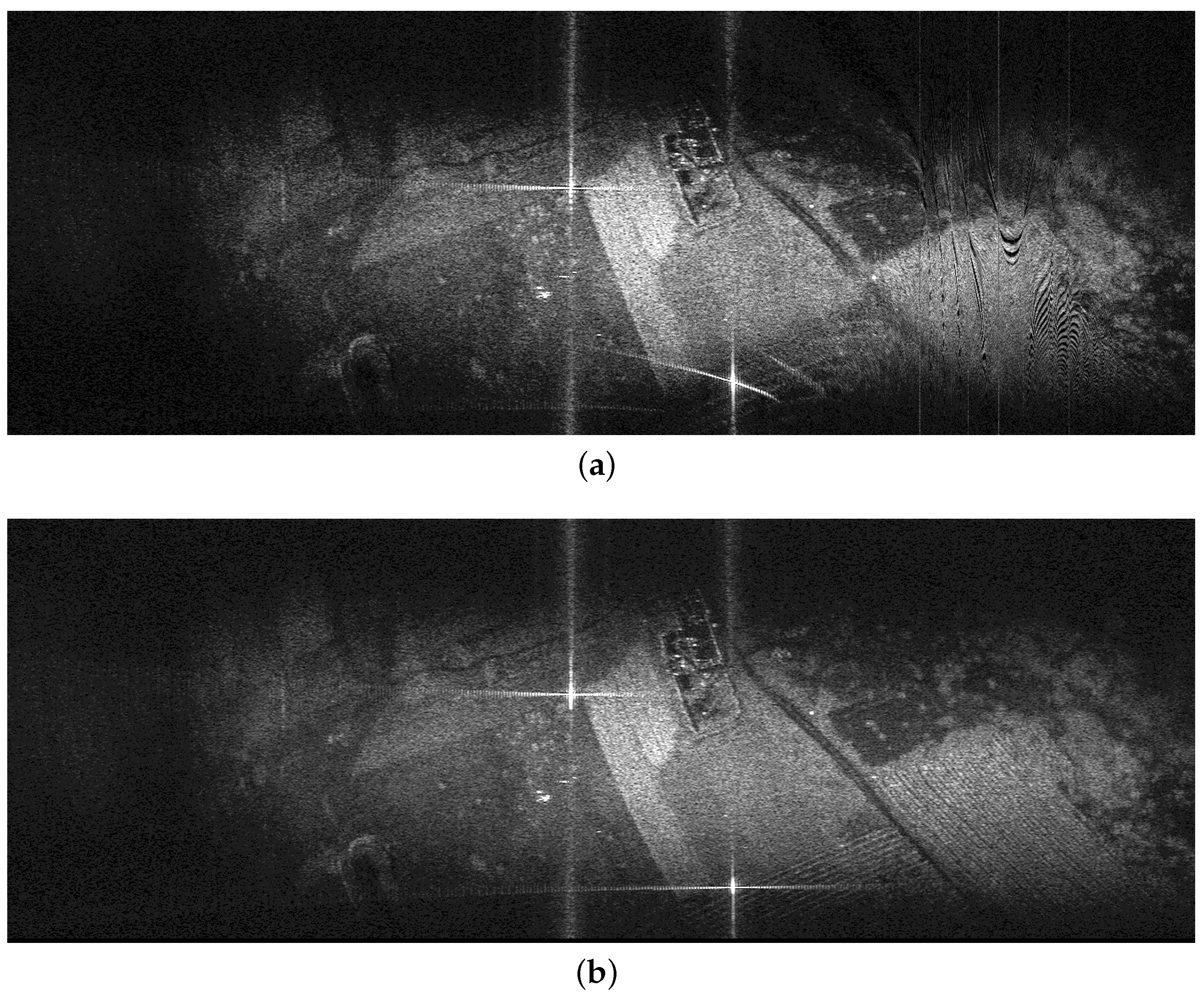
4.2. Raw Data Processing

We conducted the SAR flying experiment to obtain raw data for validation of the imaging algorithm. The raw data was obtained by UAV Bi-SAR spotlight system. The flight speeds of the transmitter and the receiver are 18 m/s and 20 m/s, respectively. The flight trajectory is approximately parallel, and the flight heights are 500 m and 400 m, respectively. The reference slant range of the scene center is 1500 m. Limited by system performance, the transmitting signal bandwidth is 50 MHz, the frequency band is Ku and the synthetic aperture time is about 3 s.
In the experimental scene as shown in Figure 16a, we can see natural scenes such as trees and grassland, as well as artificial scenes such as roads, buildings and transponders. In UAV Bi-SAR images as shown in Figure 16b, the RCS reflects the microwave characteristics of objects. Due to system limitations, the range resolution is low. SAR images of trees are very similar to optical images and are focused on point targets. Due to the presence of metal structures in buildings, their microwave reflection performance is excellent, and their RCS is high, making them strong point targets in Bi-SAR image. Roads have a strong ability to absorb radar signals, resulting in dark areas in Bi-SAR images. We placed two transponders at both ends of the grassland for imaging index evaluation. It can be seen that due to the extremely high RCS of the transponders, their response in the Bi-SAR image is the focused strong point target.
The processing results using the existing method in [31] and the proposed method in this article are shown in Figure 17a and Figure 17b respectively. Due to the instability of the UAV, limited inertial navigation system (INS) accuracy and large motion errors, phase gradient autofocusing (PGA) is used to enhance the image effect. In Figure 17b, it can be noted that the transponder targets are well focused, while the left and right road edges are very clear, in clear contrast to surrounding ground. While the image is defocused using existing method in Figure 17a, and the response results of the transponders are shown in Figure 18. The focusing effect of the transponders is shown in Figure 19. Figure 19d,h show the contour map of the transponder, and Figure 19b,f show the azimuth slice of the transponder. The transponders can be well focused using the proposed method and the evaluation results of their response are shown in Table 3. However, the comparison algorithm may encounter defocusing problems caused by large azimuth width and small time-bandwidth product caused by large motion errors in Figure 17a.
Under current parameters, due to weak azimuth spatial variability of AFP and low range resolution, defocusing and residual RCM will not occur in Figure 18. In actual processing, motion compensation and autofocusing are required, but this is not the key of this article, and specific methods will not be introduced here.

5. Conclusions

In this paper, an improved UAV Bi-SAR imaging algorithm with 2D spatial variant RCMC and ANPE is proposed. Comparing with the traditional UAV Bi-SAR frequency domain imaging algorithm, this method combines Doppler blocking with ANCS, enabling the algorithm to adapt to stronger azimuth spatial variance, thus enhancing the robustness of the algorithm, which is of great significance. Specifically, the main contribution is to combine Doppler blocking with ANCS, and to provide a detailed derivation and conclusion of the blocking criteria. Doppler blocking has the ability to correct the azimuth spatial variant range curving and RCM high-order terms. Combined with ANCS, it can eliminate the spatial variant AFP model errors, the distortion introduced by ANCS, and phase errors caused by distortion, so that the image can be well-focused in the scene with severe azimuth spatial variance. Results from simulations and UAV Bi-SAR real data processing are provided to validate the performance of the proposed algorithm. This method will support research on 3D imaging of distributed SAR systems in the future, mainly applied to 2D imaging.

Author Contributions

Conceptualization, J.Y.; methodology, J.Y. and M.K.; software, J.Y., L.L. and M.K.; validation, M.K.; formal analysis, J.Y. and M.K.; investigation, M.K.; resources, L.L.; data curation, J.Y. and M.K.; writing—original draft preparation, J.Y.; writing—review and editing, L.L., H.L., X.M. and X.S.; visualization, J.Y.; supervision, L.L. and H.L.; project administration, L.L.; funding acquisition, L.L. All authors have read and agreed to the published version of the manuscript.

Funding

This research was funded by China Postdoctoral Science Foundation (Grant No. 2022M720444) and Key Program of National Natural Science Foundation of China (Grant No. 11833001 and Grant No. 61931002).

Data Availability Statement

Not applicable.

Conflicts of Interest

The authors declare no conflict of interest.

References

  1. Auterman, J.L. Phase stability requirements for bistatic SAR. In Proceedings of the IEEE National Radar Conference, Atlanta, GE, USA, 13–14 March 1984; pp. 45–52. [Google Scholar]
  2. Wang, Y.; Ding, Z.; Li, L.; Liu, M.; Ma, X.; Sun, Y.; Zeng, T.; Long, T. First Demonstration of Single-Pass Distributed SAR Tomographic Imaging With a P-Band UAV SAR Prototype. IEEE Trans. Geosci. Remote Sens. 2022, 60, 5238618. [Google Scholar] [CrossRef]
  3. Yates, G.; Horne, A.; Blake, A.; Middleton, R. Bistatic SAR image formation. IEE Proc.-Radar Sonar Navig. 2006, 153, 208–213. [Google Scholar] [CrossRef] [Green Version]
  4. Loehner, A. Improved azimuthal resolution of forward looking SAR by sophisticated antenna illumination function design. IEE Proc.-Radar Sonar Navig. 1998, 145, 128–134. [Google Scholar] [CrossRef]
  5. Wu, J.; Yang, J.; Yang, H.; Huang, Y. Optimal geometry configuration of bistatic forward-looking SAR. In Proceedings of the 2009 IEEE International Conference on Acoustics, Speech and Signal Processing, Taipei, China, 19–24 April 2009; IEEE: Manhattan, NY, USA, 2009; pp. 1117–1120. [Google Scholar]
  6. Krieger, G.; Moreira, A. Spaceborne bi-and multistatic SAR: Potential and challenges. IEE Proc.-Radar Sonar Navig. 2006, 153, 184–198. [Google Scholar] [CrossRef] [Green Version]
  7. Cumming, I.; Bennett, J. Digital processing of Seasat SAR data. In Proceedings of the ICASSP’79—IEEE International Conference on Acoustics, Speech, and Signal Processing, Washington, DC, USA, 2–4 April 1979; Volume 4, pp. 710–718. [Google Scholar] [CrossRef]
  8. Xu, G.; Zhou, S.; Yang, L.; Deng, S.; Wang, Y.; Xing, M. Efficient Fast Time-Domain Processing Framework for Airborne Bistatic SAR Continuous Imaging Integrated With Data-Driven Motion Compensation. IEEE Trans. Geosci. Remote Sens. 2022, 60, 5208915. [Google Scholar] [CrossRef]
  9. Li, Y.; Xu, G.; Zhou, S.; Xing, M.; Song, X. A Novel CFFBP Algorithm With Noninterpolation Image Merging for Bistatic Forward-Looking SAR Focusing. IEEE Trans. Geosci. Remote Sens. 2022, 60, 5225916. [Google Scholar] [CrossRef]
  10. Xie, H.; Shi, S.; An, D.; Wang, G.; Wang, G.; Xiao, H.; Huang, X.; Zhou, Z.; Xie, C.; Wang, F.; et al. Fast factorized backprojection algorithm for one-stationary bistatic spotlight circular SAR image formation. IEEE J. Sel. Top. Appl. Earth Obs. Remote Sens. 2017, 10, 1494–1510. [Google Scholar] [CrossRef]
  11. Xie, H.; Shi, S.; Li, F.; An, D.; Xiao, H.; Xie, C.; Fang, Q.; Wang, G.; Wang, L.; Wang, F.; et al. Fast time domain approach for bistatic forward-looking SAR imaging based on subaperture processing and local beamforming. In Proceedings of the 2017 2nd International Conference on Frontiers of Sensors Technologies (ICFST), Shenzhen, China, 14–16 April 2017; IEEE: Manhattan, NY, USA, 2017; pp. 240–245. [Google Scholar]
  12. Feng, D.; Xie, H.; An, D.; Huang, X. Fast factorized back projection algorithm for spotlight bistatic forward-looking low frequency UWB SAR. In Proceedings of the IET International Radar Conference 2015, Hangzhou, China, 14–16 October 2015. [Google Scholar]
  13. Liang, Y.; Li, G.; Wen, J.; Zhang, G.; Dang, Y.; Xing, M. A fast time-domain SAR imaging and corresponding autofocus method based on hybrid coordinate system. IEEE Trans. Geosci. Remote Sens. 2019, 57, 8627–8640. [Google Scholar] [CrossRef]
  14. Tang, Y.; Xing, M.D.; Bao, Z. The polar format imaging algorithm based on double chirp-Z transforms. IEEE Geosci. Remote Sens. Lett. 2008, 5, 610–614. [Google Scholar] [CrossRef]
  15. Zhu, D.; Ye, S.; Zhu, Z. Polar format agorithm using chirp scaling for spotlight SAR image formation. IEEE Trans. Aerosp. Electron. Syst. 2008, 44, 1433–1448. [Google Scholar] [CrossRef]
  16. Rigling, B.D.; Moses, R.L. Polar format algorithm for bistatic SAR. IEEE Trans. Aerosp. Electron. Syst. 2004, 40, 1147–1159. [Google Scholar] [CrossRef]
  17. Miao, Y.; Wu, J.; Yang, J. Azimuth migration-corrected phase gradient autofocus for bistatic SAR polar format imaging. IEEE Geosci. Remote Sens. Lett. 2020, 18, 697–701. [Google Scholar] [CrossRef]
  18. Mao, X.; Zhu, D.; Zhu, Z. Polar format algorithm wavefront curvature compensation under arbitrary radar flight path. In Proceedings of the 2011 IEEE CIE International Conference on Radar, Chengdu, China, 24–27 October 2011; IEEE: Manhattan, NY, USA, 2011; Volume 2, pp. 1382–1385. [Google Scholar]
  19. Deng, H.; Li, Y.; Liu, M.; Mei, H.; Quan, Y. A space-variant phase filtering imaging algorithm for missile-borne BiSAR with arbitrary configuration and curved track. IEEE Sens. J. 2018, 18, 3311–3326. [Google Scholar] [CrossRef]
  20. Hu, C.; Zeng, T.; Long, T.; Yang, C. Forward-looking bistatic SAR range migration alogrithm. In Proceedings of the 2006 CIE International Conference on Radar, Shanghai, China, 16–19 October 2006; IEEE: Manhattan, NY, USA, 2006; pp. 1–4. [Google Scholar]
  21. Wu, J.; Huang, Y.; Xiong, J.; Yang, J. Range Migration Algorithm in Bistatic SAR Based on Squint Mode. In Proceedings of the 2007 IEEE Radar Conferenc, Waltham, MA, USA, 17–20 April 2007; IEEE: Manhattan, NY, USA, 2007; pp. 579–584. [Google Scholar]
  22. Li, Y.; Zhang, T.; Mei, H.; Quan, Y.; Xing, M. Focusing Translational-Variant Bistatic Forward- Looking SAR Data Using the Modified Omega-K Algorithm. IEEE Trans. Geosci. Remote Sens. 2022, 60, 5203916. [Google Scholar] [CrossRef]
  23. Li, C.; Zhang, H.; Deng, Y.; Wang, R.; Liu, K.; Liu, D.; Jin, G.; Zhang, Y. Focusing the L-Band Spaceborne Bistatic SAR Mission Data Using a Modified RD Algorithm. IEEE Trans. Geosci. Remote Sens. 2020, 58, 294–306. [Google Scholar] [CrossRef]
  24. Wong, F.H.; Cumming, I.G.; Neo, Y.L. Focusing bistatic SAR data using the nonlinear chirp scaling algorithm. IEEE Trans. Geosci. Remote Sens. 2008, 46, 2493–2505. [Google Scholar] [CrossRef] [Green Version]
  25. Xiaolan, Q.; Donghui, H.; Chibiao, D. Non-linear chirp scaling algorithm for one-stationary bistatic SAR. In Proceedings of the 2007 1st Asian and Pacific Conference on Synthetic Aperture Radar, Huangshan, China, 5–9 November 2007; pp. 111–114. [Google Scholar] [CrossRef]
  26. Zeng, T.; Li, Y.; Ding, Z.; Long, T.; Yao, D.; Sun, Y. Subaperture approach based on azimuth-dependent range cell migration correction and azimuth focusing parameter equalization for maneuvering high-squint-mode SAR. IEEE Trans. Geosci. Remote Sens. 2015, 53, 6718–6734. [Google Scholar] [CrossRef]
  27. Wang, Z.; Liu, M.; Ai, G.; Wang, P.; Lv, K. Focusing of Bistatic SAR with Curved Trajectory Based on Extended Azimuth Nonlinear Chirp Scaling. IEEE Trans. Geosci. Remote Sens. 2020, 58, 4160–4179. [Google Scholar] [CrossRef]
  28. Song, X.; Li, Y.; Zhang, T.; Li, L.; Gu, T. Focusing High-Maneuverability Bistatic Forward-Looking SAR Using Extended Azimuth Nonlinear Chirp Scaling Algorithm. IEEE Trans. Geosci. Remote Sens. 2022, 60, 5240814. [Google Scholar] [CrossRef]
  29. Li, S.; Zhong, H.; Yang, C.; Song, H.; Zhao, R.; Cao, J.; Xu, X. Focusing Nonparallel-Track Bistatic SAR Data Using Modified Frequency Extended Nonlinear Chirp Scaling. IEEE Geosci. Remote Sens. Lett. 2022, 19, 4007105. [Google Scholar] [CrossRef]
  30. Wu, J.; Li, Z.; Huang, Y.; Yang, J.; Yang, H.; Liu, Q.H. Focusing bistatic forward-looking SAR with stationary transmitter based on keystone transform and nonlinear chirp scaling. IEEE Geosci. Remote Sens. Lett. 2013, 11, 148–152. [Google Scholar] [CrossRef]
  31. Zeng, T.; Wang, Z.; Liu, F.; Wang, C. An improved frequency-domain image formation algorithm for mini-UAV-based forward-looking spotlight BiSAR systems. Remote Sens. 2020, 12, 2680. [Google Scholar] [CrossRef]
  32. Neo, Y.L.; Wong, F.; Cumming, I.G. A Two-Dimensional Spectrum for Bistatic SAR Processing Using Series Reversion. IEEE Geosci. Remote Sens. Lett. 2007, 4, 93–96. [Google Scholar] [CrossRef] [Green Version]
Figure 1. The relationship of UAV Bi-SAR imaging scene and slant range history.
Remotesensing 15 03734 g001
Figure 2. Taylor expansion error of slant range history of scene edge points P 1 , P 2 , P 3 , P 4 and center point P 0 using different order models. (a) Two-order model case. (b) Three-order model case. (c) Four-order model case.
Remotesensing 15 03734 g002
Figure 3. Polynomial fitting error of spatial variant RCM using different order models. (a) Polynomial fitting error of RCM using first-order model along range direction. (b) Polynomial fitting error of RCM using second-order model along range direction.
Remotesensing 15 03734 g003
Figure 4. Polynomial fitting error of spatial variant azimuth phase using different order models. (a) Polynomial fitting error of quadratic phase using first-order model along azimuth direction. (b) Polynomial fitting error of quadratic phase using second-order model along azimuth direction. (c) Polynomial fitting error of cubic phase using first-order model along azimuth direction. (d) Polynomial fitting error of quartic phase using zero-order model along azimuth direction.
Remotesensing 15 03734 g004
Figure 5. Schematic diagram of Doppler blocking.
Remotesensing 15 03734 g005
Figure 6. Azimuth spatial variant residual RCMC based on Doppler blocking. (a) RCM curve of targets in RD plane. (b) RCM curve of targets in 2D time domain plane. (c) RCM curve of targets in 2D time domain plane after the bulk RCMC. (d) RCM curve of targets in RD plane after the bulk RCMC.
Remotesensing 15 03734 g006
Figure 7. Flowchart of the proposed algorithm.
Remotesensing 15 03734 g007
Figure 8. Simulation geometry configuration. (a) The target array distribution and Bi-SAR geometry. (b) The relationship between radar beam radiation scene range and flight path is given.
Remotesensing 15 03734 g008
Figure 9. Slant range image of point targets array processed with proposed method.
Remotesensing 15 03734 g009
Figure 10. Contours of imaging scene edge targets using proposed method. (a) P 1 , (b) P 2 , (c) P 3 , (d) P 4 .
Remotesensing 15 03734 g010
Figure 11. Contours of imaging scene edge targets using existing method in [31]. (a) P 1 , (b) P 2 , (c) P 3 , (d) P 4 .
Remotesensing 15 03734 g011
Figure 12. Azimuth slice of the contour map of scene edge targets. (a) P 1 , (b) P 2 , (c) P 3 , (d) P 4 . Blue curves represent results processed using proposed method, red curves means results processed by existing method in [31].
Remotesensing 15 03734 g012
Figure 13. RCM curve of scene edge targets after RCMC using existing method in [31]. (a) P 1 , (b) P 2 , (c) P 3 , (d) P 4 .
Remotesensing 15 03734 g013
Figure 14. RCM curve of scene edge targets after RCMC using proposed method. (a) P 1 , (b) P 2 , (c) P 3 , (d) P 4 .
Remotesensing 15 03734 g014
Figure 15. Contours of imaging scene edge targets using existing method in [31] without RCM. (a) P 1 , (b) P 2 , (c) P 3 , (d) P 4 .
Remotesensing 15 03734 g015
Figure 16. Optical and UAV Bi-SAR image of observed scene. (a) Optical image, (b) UAV Bi-SAR ground image.
Remotesensing 15 03734 g016
Figure 17. UAV Bi-SAR real data imaging result. (a) Processed with existing method in [31]. (b) Processed with proposed method.
Remotesensing 15 03734 g017
Figure 18. Evaluation results of targets using existing method in [31]. (a) RCM curve of P 1 , (b) Range slice of contour map of P 1 , (c) Azimuth slice of contour map of P 1 , (d) 2D contour map of P 1 , (e) RCM curve of P 2 , (f) Range slice of contour map of P 2 , (g) Azimuth slice of contour map of P 1 , (h) 2D contour map of P 1 .
Remotesensing 15 03734 g018
Figure 19. Evaluation results of targets using proposed method. (a) RCM curve of P 1 , (b) Range slice of contour map of P 1 , (c) Azimuth slice of contour map of P 1 , (d) 2D contour map of P 1 , (e) RCM curve of P 2 , (f) Range slice of contour map of P 2 , (g) Azimuth slice of contour map of P 1 , (h) 2D contour map of P 1 .
Remotesensing 15 03734 g019
Table 1. Simulation system parameters of UAV Bi-SAR.
ParametersValuesUnits
Carrier frequency15GHz
Pulse duration3µs
Range bandwidth800MHz
Sampling frequency1200MHz
Pulse repetition frequency1000Hz
Synthetic aperture time6s
Scene center coordinate(2000, 500, 0)m
Transmitter coordinates(1050, −550, 600)m
Receiver coordinates(850, −650, 450)m
Transmitter velocity25m/s
Receiver velocity30m/s
Table 2. Evaluation results of imaging simulation index of point targets.
PointsRange Resolution (m)Azimuth Resolution (Hz)Range PSLR (dB)Azimuth PSLR (dB)Range ISLR (dB)Azimuth ISLR (dB)
P10.16410.1484−12.97/−13.98−13.32/−12.35−10.54−9.99
P20.17190.1458−13.14/−13.63−13.28/−13.11−10.37−10.18
P30.17190.1458−13.82/−13.06−13.12/−13.18−10.40−10.16
P40.16410.1484−13.61/−13.14−13.16/−13.28−10.33−10.20
Table 3. Evaluation results of UAV Bi-SAR real data imaging using proposed method.
PointsRange Resolution (m)Azimuth Resolution (Hz)Range PSLR (dB)Azimuth PSLR (dB)Range ISLR (dB)Azimuth ISLR (dB)
P12.63670.2051−13.64/−14.01−13.41/−13.04−11.97−10.15
P22.69530.2014−13.84/−13.44−13.39/−13.04−11.37−10.20
Disclaimer/Publisher’s Note: The statements, opinions and data contained in all publications are solely those of the individual author(s) and contributor(s) and not of MDPI and/or the editor(s). MDPI and/or the editor(s) disclaim responsibility for any injury to people or property resulting from any ideas, methods, instructions or products referred to in the content.

