
Comparison of Freshwater Content and Variability in the Arctic Ocean Using Observations and Model Simulations

1
School of the Earth, Ocean, and Environment, University of South Carolina, Columbia, SC 29208, USA
2
Naval Research Laboratory, Stennis Space Center, Kiln, MS 39556, USA
*
Author to whom correspondence should be addressed.
Remote Sens. 2023, 15(15), 3715; https://doi.org/10.3390/rs15153715
Submission received: 8 June 2023
/
Revised: 21 July 2023
/
Accepted: 23 July 2023
/
Published: 25 July 2023
(This article belongs to the Special Issue Advances in Remote Sensing of Ocean Salinity)
Abstract
:Freshwater content (FWC), generally characterized in the Arctic Ocean by salinities lower than 34.8 psu, has shifted in both quantity and distribution in recent decades in the Arctic Ocean. This has been largely driven by changes in the volume and salinity of freshwater sources and the direction and magnitude of major currents. In this study, we analyze the variability in FWC and other physical oceanographic variables from 1993 to 2021 in the Arctic Ocean and Beaufort Gyre (BG) using in situ and remote sensing observations and five ocean models and reanalysis products. Generally, ocean models and reanalysis products underestimate FWC in the BG when compared with observations. Modeled FWC and sea surface height (SSH) in the BG are well correlated during the time period and are similar to correlations of the observational data of these variables. ORAS5 compares best to EN4 salinity over the entire study period, although GLORYS12 agrees well pre-2007 and SODA post-2007. Outside the BG, consistency between modeled SSH, FWC, and limited observations varies between models. These comparisons help identify discrepancies in ocean model and reanalysis products while highlighting areas where future improvements are necessary to further our understanding of Arctic FWC. As observations are scarce in the Arctic, these products and their accuracy are important to studying this dynamic and vulnerable ocean.
1. Introduction
The Arctic Ocean’s stratification and vertical density distribution are primarily dependent on salinity due to the relatively homogenous low water temperatures and consequently low thermal expansion coefficient. The surface and halocline layers in particular are salt stratified with fresher, less dense waters on top [1]. These freshened waters, often defined as water with salinity less than 34.8 psu in the Arctic Ocean, play an important role in local circulation and preventing mixing. These waters separate the sea surface from relatively warm, salty Atlantic Water below, therefore influencing the sea-ice formation. The upper ocean also has a hand in linking the Arctic Ocean to the global circulation, potentially slowing Atlantic meridional overturning circulation if large volumes of freshened waters are released, and therefore potentially having far-reaching effects on the global climate [2]. Freshwater content (FWC), corresponding to the vertical integration of the salinity deficit relative to a reference salinity (here 34.8 psu), varies in the Arctic Ocean due to changes in both the amount of freshwater available and the uneven distribution of it across the Arctic [3]. Freshwater inputs include river runoff, glacial and sea-ice melt, Pacific water inflow, and net precipitation, while the distribution of these waters varies with winds, currents, and mixing processes.
The Beaufort Gyre (BG) in the Canadian Basin is a predominantly anticyclonic upper ocean feature in the mean circulation of the Arctic Ocean that includes an FWC maximum. On average, the BG holds ~23,000 ± 2000 km3 of the Arctic’s 100,000 km3 of FWC (~25%) [4,5], and FWC increased approximately 6400 km3 from 2003 to 2018 [3]. The gyre is driven by the Beaufort High, the mean atmospheric high-pressure pattern in the region, which causes anticyclonic wind stress and the Ekman convergence of surface low salinity water. This leads to the doming of the sea surface height (SSH) and deepening of the isopycnals in the center of the gyre. While the surface is ice-covered, the freshwater accumulation is largely equilibrated by feedback among Ekman forcing associated with the wind-driven spin-up of the ice and upper ocean, and spin-down by internal ice stress where friction slows the ice enough to reverse the direction of the ice-ocean stress and cause Ekman divergence [6]. This process was referred to as the ice-ocean governor (IOG) [7]. Additionally, eddy diffusion dissipates energy in the gyre on timescales of years to decades [8] and becomes the primary counter to Ekman-driven accumulation in the absence of ice cover. Changes in the BG FWC due to the IOG can be as much as five times stronger than those due to eddy fluxes [9], except in the presence of the continental slope where eddy dynamics dominate [10]. Understanding the balance between wind stress, eddies, and the IOG in the BG will become increasingly important as the sea-ice concentration and multi-year sea ice continue to decrease, reducing the effect of the IOG and therefore the response time of the BG equilibrium. FWC in the BG can also be affected by changes in its freshwater inputs, such as shifts in freshwater pathways, changes in the amount of Pacific Ocean inflow taken up, or anomalously warm years leading to increased sea-ice melt [11,12].
Variability in the BG FWC is also related to the Arctic Oscillation (AO). The AO is the leading empirical orthogonal function (EOF) of the Northern Hemisphere surface atmospheric pressure variation [13]. When the AO is in a positive phase, a low-pressure pattern over the east longitudes of the Arctic Ocean drives cyclonic winds and changes in near surface circulation, consistent with the cyclonic mode [14]. The cyclonic mode features strengthened cyclonic surface circulation on the Eurasian side of the Arctic Basin, which diverts Eurasian runoff to the Canada Basin where it expands the Beaufort Sea halocline and is partly responsible for strengthening the BG [15]. Related to this, the cyclonic mode includes an intensified BG along the Canadian margin of the ocean and a Transpolar Drift (TPD) that is rotated counterclockwise and shifted towards North America. The cyclonic mode is related to the winter (NDJFMA) AO with a 1-year lag and has become more prominent since 1990 due to a positive shift of one standard deviation in the AO [16]. The resulting more cyclonic and divergent circulation has resulted in increased sea-ice export during positive AO years [16,17].
In spite of the importance of salinity and FWC to Arctic Ocean dynamics, making in situ observations in the area remains a challenge, and remote sensing, ocean modeling, and ocean reanalysis products are thus increasingly important to studying the region as they can fill in spatial and temporal gaps in measurements. Ocean models and reanalyses have been validated for parameters such as temperature, salinity, and sea-ice in the Arctic for a variety of time scales and regions [18,19,20,21], but there are still limitations in their abilities and usefulness. Satellite salinity and altimetry have been used as mechanisms to estimate FWC remotely [15,22,23,24], although there are also limitations to those datasets. Satellite salinity retrievals are restricted to ice-free regions and have large uncertainties in cold water, for example [25]. Evaluating our simulations of SSS and SSH will therefore allow us to assess FWC and its relationships to other parameters more accurately in the Arctic Ocean and improve predictions. It should also be noted that access to in situ measurements in areas such as the Russian shelf is very limited relative to measurements in west longitudes [26]. This emphasizes the importance of model simulations for the region, but to the extent they depend on climatology, wide variations among model results are expected.
In this paper, we present a multi-product analysis comparing salinity and related variables among in situ observations, satellite data, ocean model simulations, and reanalysis products to explore our understanding of FWC, its changes, and related variables. Focus is placed on the well-studied BG region, as well as on the change in long-term trends of FWC pre- and post-2007 due to the AO. With this paper, we aim to evaluate different ocean model products in the Arctic, especially when analyzing long-term trends. Our study covers January 1993–December 2021 depending on the availability of the products used. The products have varying spatial and temporal scales, as described in Section 2, along with our methods. Section 3 outlines the research results which are then discussed in Section 4. A conclusion is provided in Section 5.
2. Materials and Methods
2.1. Observations
2.1.1. Satellite Data
Three satellite salinity products were utilized in this work in conjunction with the in situ, ocean model, and reanalysis data (Section 2.2). Soil Moisture and Ocean Salinity (SMOS) SSS Version 3.1 in the Arctic [27], provided by the Barcelona Expert Center (BEC), has a spatial resolution of 25 km on an Equal Area Scalable Earth-grid 2.0 and a temporal resolution of 3 days from 2011 to 2019. Soil Moisture Active Passive (SMAP) version 5.0 Level 3 SSS was also used [28]. SMAP salinity data are produced by Remote Sensing Systems and sponsored by the National Aeronautics and Space Administration’s (NASA) Ocean Salinity Science Team [29]. This product provides data from the period 2015–2021 with 0.25° (~28 km) spatial resolution and an 8-day running mean applied for full spatial coverage [28]. The final satellite salinity product used in this study is the Multi-Mission Optimally Interpolated Sea Surface Salinity (OISSS) Level 4 version 1.0, produced by the International Pacific Research Center (IPRC) of the University of Hawaii at Manoa [30] in collaboration with the Remote Sensing Systems (RSS), Santa Rosa, California. OISSS data are provided as weekly means of three satellite missions (NASA’s Aquarius, NASA’s SMAP, and BEC’s SMOS) optimally interpolated during the period 2011–2020 with a spatial resolution of 0.25° (~28 km) [31]. The SSS estimate is generated using the same optimal interpolation designed for salinity processes in the Upper Ocean Regional Study, but with an additional step to correct SSS retrievals for large-scale satellite biases with respect to in situ measurements [32].
Monthly Arctic Ocean dynamic ocean topography (DOT) from Armitage et al. [24] was analyzed during the period 2003–2014. This product was constructed by Armitage et al. from Envisat and CryoSat-2 data, with SSH relative to the WGS84 ellipsoid. DOT was computed by subtracting the GOCO03s geoid from the SSH. The GOCO03s geoid is a combined satellite-only geoid constructed from the Gravity Field and Steady-State Ocean Circulation Explorer and Gravity Recovery and Climate Experiment data, among others, but uses no altimetry data. The DOT dataset is on a 0.75° × 0.25° longitude/latitude grid, covering latitudes below 81.5°N, and the resulting grid is then smoothed with a Gaussian filter with a standard deviation of 100 km and a radius of three standard deviations. It was found by Armitage et al. [24] to agree well with both tide gauge and ITP data and has since been used in other analyses of the Arctic [33,34].
2.1.2. In Situ Data
The Met Office Hadley Centre’s “EN” series analysis product, version 4.2.2 (EN4), using Gouretski and Reseghetti [35] XBT corrections and Gouretski and Cheng [36] MBT corrections, provides monthly ocean salinity analyses which are produced using the optimal interpolation of data from Argo floats, Global Temperature and Salinity Profile Program, and the World Ocean Database’ 18 from 1900 to present [37]. EN4 also includes the Arctic Synoptic Basin-wide Oceanography, which is a compilation of other profiles, including the Beaufort Gyre Exploration Project, with the intention of improving data coverage in the Arctic [37]. The analyses are on a 1° horizontal resolution with 42 depth levels starting at 5 m depth. It is a product commonly used in ocean reanalysis products, including Ocean Reanalysis System 5 (ORAS5) and the Global Ocean Reanalysis and Simulations (GLORYS12), discussed below [38]. There are potential degradation issues in less sampled regions that could lead to inaccuracies in the EN4 product [38], though EN4 is commonly used as a reference to other ocean products [18]. EN4 provides a field of observation weights to inform users how much a value has been determined by observations (closer to 1) versus background fields (closer to 0). The mean weights on salinity values on the Russian Shelf indicate that they are primarily background field-based, with values between 0.2 and 0.3, while the average for the BG region is 0.5. The Nordic Seas, in contrast, have an average weight of 0.8.
2.1.3. Arctic Oscillation Index
The monthly mean AO index from the National Oceanic and Atmospheric Administration’s Climate Prediction Center was used in this paper (https://www.cpc.ncep.noaa.gov/products/precip/CWlink/daily_ao_index/monthly.ao.index.b50.current.ascii, accessed on 12 May 2022). The AO index is constructed by projecting the 1000 mb height anomalies poleward of 20°N onto the leading mode of EOF analysis of monthly mean 1000 mb height during the period of 1979–2000. To find the winter index of each year, the November and December values of the previous year were averaged with January through April values of the given year.
2.2. Ocean Model and Reanalysis Products
A summary of model and reanalysis product characteristics used in this work is provided in Table 1, with in depth descriptions in the following paragraphs.
NASA’s Estimating the Circulation and Climate of the Ocean (ECCO) version 4 release 4 (v4r4) estimates monthly salinity, SSH, and sea-ice data for 1992–2017 [39]. Version 4 is the first version of ECCO to include the Arctic in its model and has been used in several studies of the region [22,40,41]. The grid used in v4r4 is called the Lat-Lon-Cap 90 (LLC90) grid to avoid the limitations of the regular cubed-sphere grid and better include the Arctic [41], with the original horizontal resolution varying spatially from 22 km in the polar regions to 110 km at midlatitudes. The model has 50 depth levels starting at 5 m depth. ECCO is constrained by a variety of profiles and gridded datasets and uses Fekete et al., 2002 [42] as well as the seasonal climatology of river runoff data [40]. The ECCO estimate is one of few products with data over a long duration in the Arctic and has been shown to be approaching the observational accuracy at high latitudes and decadal time scales [18].
Daily Nucleus for European Modelling of the Ocean version 3.1 (NEMOv3.1) ocean modeling framework with the Louvain-la-Neuve Sea Ice Model (LIM2) salinity, SSH, and sea-ice data from the period 2016–2021 is used. The atmospheric forcings are from the European Centre for Medium-Range Weather Forecasts (ECMWF) Integrated Forecast System, and forcings also include updated monthly climatological river discharge from Dai et al., 2009 [43]. The output has an original resolution of 0.083° based on the tripolar ORCA grid with a horizontal resolution of 9 km at the equator, 7 km at mid-latitudes, and 2 km toward polar regions. The model has 50 vertical levels starting at 0.5 m [44]. The NEMO framework is widely used in oceanographic modeling and Arctic studies [11,45,46].
Data from the Polar Science Center of University of Washington’s Applied Physics Laboratory coupled ice-ocean model, Marginal Ice Zone Modeling and Assimilation System (MIZMAS), were also used in this work [47]. MIZMAS combines the Los Alamos National Laboratory’s Parallel Ocean Program model and a thickness and enthalpy distribution sea-ice model, adapted from the Pan-Arctic Ice-Ocean Modeling and Assimilation System (PIOMAS) [48]. The model’s forcings also includes a monthly climatology of river runoff to the Arctic Ocean and Bering Sea. MIZMAS produces the daily salinity, SSH, and sea-ice estimates from the period 2012–2017 on a grid based on a generalized orthogonal curvilinear coordinate system centered on Alaska. The MIZMAS data retrieved was limited to the region around the system’s center in the Beaufort Sea due to the size of the dataset and our focus on the BG region. The model has 40 vertical layers starting at 0.5 m depth. This model was designed to address marginal ice zone processes [49] with a unique emphasis on ice processes and is therefore valuable for analyzing the FWC in the Arctic Ocean.
We use monthly salinity, SSH, and sea ice data from the European Centre for Medium-Range Weather Forecasts’ (ECMWF) ORAS5 as well [50]. ORAS5 is an eddy-permitting ice-ocean ensemble reanalysis product which uses the NEMOv3.4 ocean model coupled to the LIM2 sea-ice model, and ERA-Interim atmospheric reanalysis forcing from 1979–2014, and ECMWF Numerical Wave Prediction using revised CORE bulk formulas after 2015 [51]. ORAS5 covers from 1979 to 2018 and is originally on an ORCA 0.25° grid. The product has 75 vertical layers starting at 0.5 m depth. ORAS5 is a product with nearly four decades of data available in the region and has been shown to be approaching observational accuracy at decadal timescales and high latitudes [18]. ORAS5 was also recently used to study the Arctic FWC by Hall et al. [21] and was demonstrated to be one of the better performing models in the region.
Mercator Ocean International’s GLORYS12 is a global eddy-resolving reanalysis product in the framework of Copernicus Marine Environment Monitoring Service (CMEMS) [52]. GLORYS12 also uses NEMO and LIM2 as its ocean and ice model components, driven at the surface with ERA-Interim atmospheric reanalysis, and satellite-based, large-scale corrections are applied to known flux biases. The product has daily salinity, SSH, and sea-ice data from 1993–2019 at 0.083° original horizontal resolution and 50 depth layers starting at 0.5 m depth. A variety of in situ and satellite data, including altimetry, are assimilated using a reduced-order Kalman filter, but no satellite salinity products are used [53]. This version is an improvement on previous versions in several areas, including an update of Dai et al., 2009 [43], runoff data with freshwater fluxes from polar ice sheets, and a better representation of the variability in salt content [54].
Also used was the University of Maryland’s Department of Computer, Mathematical, and Natural Science’s eddy-resolving reanalysis product, Simple Ocean Data Assimilation (SODA) version 3.12.2, based on the Modular Ocean Model, version 5 (MOM5.1) [55]. This version utilizes the ocean component of the Geophysical Fluid Dynamics Laboratory-coupled model (GFDL CM2.5), including the GFDL Sea Ice Simulator, and using Japanese 55-year flux corrected atmosphere reanalysis (JRA-55DO) forcing and COARE4 bulk formula. The JRA-55DO version was chosen as several other products in this study use ECMWF atmospheric forcings. As the choice of atmospheric reanalysis has strong effects, particularly on sea ice, we wanted to diversify the products represented in this study. Salinity, SSH, and sea-ice data are available as monthly averages from 1980 to 2017 and gridded onto a uniform 0.5° Mercator grid with 50 vertical levels starting at 5 m depth. SODA also uses the monthly climatological river discharge data from Dai et al., 2009 [43] among its forcings. SODA is a product with a long duration of data in the Arctic and is approaching observational accuracy at high latitudes and decadal time scales [18].
2.3. Methods
Sea surface salinity (SSS), SSH, and sea-ice data from all products except satellite salinity were interpolated using a natural neighbor interpolation method onto a 25 km polar stereographic grid for comparison. FWC was calculated on native grids and the resulting 2D values were also naturally interpolated onto the polar stereographic grid, as it saved more unique features between models. Salinity with depth was linearly interpolated, as natural interpolation is not a 3D method. In observations of FWC calculated from Ice-Tethered Profilers (ITPs) [3], an error resulting from extending the salinity at the depth of the shallowest measurement (approximately 7 m) to the surface was nonexistent in the winter due to the deeper mixed layer and only ~0.5 m in the summer melt season. Similarly, the differences in FWC between the models with salinities starting at 0.5 m versus 5 m should be negligible for our purposes. The salinity at the first depth level of each product was also used as SSS. Mixed layer depths calculated from over 21,000 measurements found the average summer minimum mixed layer depth in much of the Arctic, including the BG, to be ~8 m regardless of the ice cover [56]. While there are some shallower mixed layer depths, extending the model products’ salinities from 0.5 m or 5 m to the surface depending on the product should result in minimal error in the open ocean. Sea-ice extent was defined using the commonly used National Snow and Ice Data Center’s definition, where the ice covered area has a sea-ice concentration greater than 15% [57].
Liquid FWC quantifies the vertically integrated salinity anomaly from a reference salinity (Sref), chosen here as 34.8 psu. The choice of reference salinity can affect freshwater calculations, especially fluxes [58,59], and varies between studies. The salinity value of 34.8 psu was the climatological mean of the Arctic Ocean in 1983 and has been used as Sref in several other studies for FWC calculations [2,5]. To make our results more comparable to other studies, 34.8 psu is sufficient for our purposes. We calculated FWC (m) using the same method as Carmack et al. [60], Fuentes-Franco and Koenigk [61], and Dewey et al. [62], with the equation:
where S(z) is the salinity (psu) at a depth of z. We integrated FWC from the initial depth for each product (init) to the depth of the 34.8 psu isohaline (D). Integrating this value over a horizontal area yields the total freshwater volume (FWV; km3). FWV calculated for the BG (i.e., “BG box”, BG region) refers to the area from 70.5 to 80.5°N and 130 to 170°W, similar to other studies of the gyre [11,21,34,63,64].
Time series trends were found from the slope of the lines fitted to the data. Correlation was determined using Pearson’s linear correlation coefficient, with its significance determined by p values less than 0.01.
3. Results
3.1. Sea Surface Variability and Connection to Freshwater
SSS is compared to satellite SSS over September and April of 2017 to focus on general differences in the Arctic Ocean, and the BG region (Figure 1 and Figure 2) [56]. September (April) was chosen as it is the month of minimum (maximum) sea-ice extent on average. This provides the maximum satellite data for comparison in September, and large variability in SSS to compare to ice extent. The two years 2016 and 2017 were the only two covered by every product compared, and as 2016 was a year of anomalously low ice, 2017 was chosen to compare the SSS and sea-ice extent to contrast some capabilities of the models [65]. ECCO is the only model simulation used here that assimilates satellite-derived salinity and uses the Aquarius product [39].
In September 2017, the Canadian Basin tends to be fresher than 30 psu in products other than NEMO (Figure 1). The salinity of Pacific inflow in the Chukchi Sea shown here is generally between 31 and 33 psu, and the Atlantic side is typically more saline than 33 psu. The salinity and extent of the freshwater input from rivers on the Russian shelf varies. Much of the data in the central Arctic Ocean basin are lost to sea-ice cover in satellite products, and the resolution on EN4 is relatively coarse and unreliable due to there being virtually no in situ observations available in this area, so the fine details seen in the modeled salinity are difficult to compare to. For example, NEMO shows a tongue of high salinity values along the shelf north of the Laptev Sea, which is not seen in the observations. MIZMAS shows a very fresh signal in the southeast of the BG and is noticeably fresher than any other product in the northern Canadian Basin. ECCO also overestimates salinity on the Russian shelf compared to both satellites and other models, and its salinities in the BG region are not representative of the maximum (32 psu) through the Bering Strait nor the minimum (25 psu) near the BG center seen in observation-based products. NEMO and GLORYS12 only show a low-salinity signal immediately at the mouth of the Mackenzie River in the southeast of the BG box, and not the rest of the BG. ORAS5 and SODA show the lowest salinity limited to the BG and a high salinity in the Bering Strait, more closely agreeing with satellite observations and EN4.
Due to the greater ice cover, satellites are unable to represent most of the Arctic’s salinity in April, which further limits the ability to validate the models (Figure 2). All models and reanalyses show a much higher SSS, with Atlantic water reaching farther over the central basin. The BG region in April is saltier in all products as well, and particularly in MIZMAS. The fresh Russian Shelf waters also extend less far, especially in EN4, ORAS5, and SODA. In ECCO, the fresher water on the Russian Shelf nearly disappears in April compared to September, but the values in the BG region are closer to EN4 than in September. MIZMAS shows the saltiest Pacific Water inflow in April following the Russian coast west, differing from its September values and matching EN4 more closely. The differences between the April and September SSS values in our paper are also not consistent across the models with shallower or deeper initial depths. SODA shows a very similar SSS change to ORAS5, despite having a deeper initial depth, while ECCO changes a similar amount to NEMO and GLORYS12, even though the salinity values are fresher. In summary, many models show a 1–3 psu higher SSS in the BG than EN4, consistent with Hall et al. [21].
The sea-ice extent in September and April of 2017 is also compared between models (Figure 1 and Figure 2). In September, NEMO, MIZMAS, ORAS5, and GLORYS12 show very similar lines of sea-ice extent on the Pacific side of the Arctic, which follow with the patterns of data availability in the satellite salinity products due to sea-ice cover. ECCO shows a large tongue of melt toward the pole compared to the other products while still covering much of the BG. SODA shows a uniquely high amount of ice coverage in the BG. In ORAS5, SODA, and to a lesser extent MIZMAS, the low salinity in the center of the gyre follows the sea ice line across the BG as it does in the observations [62]. ECCO shows low salinity farther north past the ice edge. The ice extent lines are consistent on the Atlantic side, and although the salinity gradient across the edge differs between models, the ice edge generally straddles the line between the saltiest Atlantic waters and the fresher basin waters closely. This pattern on the Atlantic side of the Arctic also occurs in April, while the Pacific side is completely covered in sea ice.
FWC can be used as a measure of salinity anomaly with depth, and it shows changes in freshwater accumulation and release. FWC is calculated from all salinity products from a Sref of 34.8 psu, as described in the methods (Section 2), and are averaged over 2017 for each salinity product (Figure 3). Again, 2017 is chosen as 2016 and 2017 are the years of data availability for every product, but 2016 experienced anomalously low ice, and so would potentially have anomalously low salinity. Therefore, 2017 gives a good snapshot of recent salinity values across all products. As expected, FWC is high on the fresher, Pacific side of the Arctic, and lower on the Atlantic side. EN4 shows a strong FWC maximum in the BG region, as well as a secondary maximum to the west of the BG in the Chukchi Borderland-Eastern Makarov Basin region. There are also small amounts of FWC along the Russian shelf and in the Eurasian Basin. ECCO, shows 20 m of average FWC compared to EN4′s 23 m. NEMO has a similar maximum to EN4 [3]. MIZMAS has both a unique, Arctic-specific domain and a unique “L” shaped pattern of FWC with a southern edge farther from the Alaskan coast than other products. ORAS5 and SODA have maximums of 26 m, while GLORYS12′s maximum is only 21 m. EN4 is included in ORAS5′s forcings, so the agreement is expected. SODA also shows a uniquely high amount of FWC along the Russian Shelf, particularly near the Kolyma River in the East Siberia Sea and the Lena River in the Laptev Sea. ECCO and SODA also show large amounts of FWC on the Chukchi Borderland like EN4. GLORYS12 has the largest amount of FWC in the Eurasian Basin.
SSH changes are closely tied to salinity in the Arctic due to halosteric effects, and this relationship is well studied [15,23,24]. With the thermal component making a negligible contribution to steric SSH changes in the BG, the high SSH in the mean of each product spatially matches the mean FWC on the Pacific side of the Arctic very closely. The different model representations of this relationship are further explored here by mapping the correlation between FWC and SSH (Figure 4 and Figure 5). As EN4 is only a temperature and salinity product, the satellite DOT product from Armitage et al. [24] was used for comparison to EN4, although the coverage does not extend beyond 81.5°N (Figure 4a). This correlation was run from 2003 to 2014, matching the temporal extent of the DOT dataset. The correlation between EN4 and the DOT is very strong (0.8–0.85) in the center of the Beaufort Gyre (Figure 4a). However, the correlation is very low on the Russian Shelf. This is possibly due to the low number of salinity observations in EN4 in the region, although since a similar low correlation on the Russian Shelf is shown in several models, this may instead also be due to ocean dynamics in the region (Figure 5).
In the models and reanalyses, the expected correlation is strongest in the BG, but spatial patterns outside of the Canadian Basin vary. Many products have a high correlation between FWC and SSH beyond the extent of the DOT dataset in the Makarov and Eurasian Basins. As these correlations are based on each products’ respective data availabilities, the exact length of time the correlation is tested for variance. As such, the correlations values are representative of each product’s internal agreement, instead of a direct comparison between products. ECCO’s maximum correlation is lower than the other products, but still very high (0.9 compared to 0.95 in other products). ORAS5 and SODA (Figure 5g,k) have areas of lower correlation near the North Pole, while MIZMAS (Figure 5e) has a larger and more southern low correlation hole, continuing even into the northern BG. All products have a lower correlation between FWC and SSH around the East Siberian Sea, but ECCO, NEMO, ORAS5, and SODA show a tongue between the Laptev Sea and the Makarov Basin. Overall, the better agreement on the correlation between the model and observed SSH in the BG compared to other areas may reflect the greater number of in situ observations supporting the models in the BG than elsewhere [26].
SSS is also related to the freshwater accumulation of the Arctic, as the freshwater sources affecting the upper tens of meters of liquid FWC such as precipitation, runoff, and ice melt also alter SSS. Because of this, SSS was examined as a proxy for FWC using ECCO v4r3 by Fournier et al. [22]. The two variables were found to have a close inverse relationship, especially on the Russian Shelf due to the riverine input. A strong negative correlation (−0.95 to −0.8) on the Russian Shelf is also seen across all products in our work (Figure 4 and Figure 5). Most products also show a negative correlation in the Chukchi Sea where there is an input of relatively fresh Pacific water. GLORYS12, SODA, and to a lesser degree ORAS5 also show a defined area of negative correlation in the Eurasian Basin. EN4 (Figure 4b) has a shape of weak anticorrelation in the BG similar to the one of correlation between FWC and SSH, likely as sea ice diverted to the center of the gyre melts there. ECCO and SODA (Figure 5b,l) show a similar pattern, and MIZMAS and ORAS5 (Figure 5f,h) to a weaker extent. All products also have areas of little to no SSS correlation in the Canadian Basin, and especially on its edges. Fournier et al. [22] compared SSS to steric SSH, and noted a similar disagreement around the BG. They posited that it was due to the BG’s sea level changes being dominated by Ekman pumping fluctuating the halocline depth, which would not show up in the SSS signal. FWC also enters the BG at depth from deeper density contours shoaling in the Chukchi Sea and incorporating relatively fresh Pacific Water into the BG [66,67], so FWC can vary even without changes in SSS. NEMO (Figure 5d) is the least anticorrelated on the Pacific side of the Arctic. As NEMO is only run from 2016 to 2021, and Pacific water inflow has been both increasing and freshening from 1990 to 2019 [68], it is possible that the changes in FWC during the NEMO period were simply not represented by changes in SSS, particularly to the west of the BG where these waters enter.
3.2. Comparison of Beaufort Gyre Properties
The product comparisons of FWC differ greatly outside the BG, so the next section of analysis will focus on each product’s performance within the BG. Focus is given to FWV, as well as the sea-ice variability between models to compare the causes of freshwater accumulation. The FWC is integrated over the BG box in every month to obtain the FWV of each salinity product, and each month is compared to the same month’s FWV from EN4 (Figure 6). The data are also broken by different time periods. The first period is before July 2007, the second from July 2007 to December 2010, and the third after 2010. The exact length of these periods varies by data availability for each product. These periods were chosen to represent shifts in freshwater accumulation based on the AO Index and will be discussed more in the next section (Section 3.3).
All the models, with the exception of ORAS5, underestimate BG FWV relative to EN4 (Figure 6). Average deficits range from 2 to 4 × 10³ km3, consistent with modelled salinities being generally greater than EN4 climatology. Beyond the mean FWV deficiencies for each model, the correlation between the BG FWV of EN4 and other salinity products also varies. For ECCO, the post-2010 time period is a broader cluster than the pre-2007, although the correlation of 0.85 for the whole time period is significant. NEMO changes very little over its limited time period, while the FWV values in EN4 comparatively increase in 2018 and 2019, so NEMO is essentially uncorrelated with EN4. MIZMAS is slightly better in this regard, but behaves similarly, with a near horizontal trend line and a correlation that is not significant. These two models are likely poorly correlated due to the short amount of time being represented, as well as the limitations of the box-sum method for FWV, which will be discussed further in Section 4. ORAS5′s FWV is the closest to that of EN4′s of all products, with both a significant correlation of 0.90 and minimal FWV deficit. However, as mentioned previously, EN4 is included in its forcings, so closer agreement is expected, and may not strictly be indicative of ORAS5′s inherent accuracy. ORAS5 has been compared to another in situ salinity measurement in the BG by Hall et al. [21], however, and was found to be in good agreement with it as well. GLORYS12 is also highly correlated (0.88), although the FWV deficit is larger and worsens with time. The pre-2007 points cluster around the 1:1 line more closely. The 2007–2010 points are also well mixed with the post-2010 period’s, indicating that GLORYS12 did not show as much FWC accumulation in BG as EN4 during those two periods compared to ECCO or SODA, where each period is more distinctly plotted. SODA also has a high correlation of 0.82, but unlike GLORYS12, its performance improves with time. The pre-2007 points are clustered farther from the 1:1 line than the post-2010.
Time series of BG FWV and sea-ice volume from each model are also used to visualize these differences (Figure 7b,c). Again, with the possible exception of ORAS5, the modeled FWV results are less than those seen in EN4. SODA’s FWV values converge towards those of EN4 and ORAS5 over time, while GLORYS12 varies more after 2007. Strong seasonal variability is shown in ECCO and MIZMAS, with SODA and GLORYS12 showing smaller changes. ECCO, MIZMAS, and to a lesser extent NEMO consistently underestimate BG FWV throughout the records, although NEMO and MIZMAS have an FWC extending west or north beyond the BG box region, so the FWV shown here is an inexact estimation of their total FWV.
The volume of BG sea ice in each model was also compared (Figure 7c), and generally decreases with time across all products. While these values are likely 10–15% greater than the corresponding solid FWC due to sea-ice salinity, the values are close to those found in the BG region’s sea ice FWC equivalent in Proshutinsky et al. [3]. Furthermore, the seasonal variations in SIV are essentially the inverse of the seasonal variations in liquid FWC. The seasonal peaks are consistent with observations, with the minimum being in the summer, usually September, and the maximum being in April. This inverse character of the seasonal cycles of liquid FWC and SIV is consistent with the finding that, over the summer melt season, the freshening of the upper ocean in the BG Seasonal Ice Zone could be accounted for by the loss in sea ice during the ice edge retreat [62]. The residual SIV plus liquid FWC (Figure 7d) shows a smaller seasonal signal than the constituent components, with the largest in MIZMAS and the smallest in ECCO, with a maximum in winter to early spring consistent with winter spin up of the BG [60]. The SIV values are fairly consistent across products compared to FWV values, so the combined time series shows a similar spread across products to the FWV alone.
3.3. Influence of 2007 AO Event
The AO can have a large influence on the dynamics of FWC in the Arctic Ocean, as described in many previous works [15,69]. For our comparison, we divided the range from 1993 to 2021 into three main periods visible in the FWC data from EN4 that roughly align with changes in the AO: one period from 1993 to July 2007, where the FWV in the BG was relatively stable, a second period from July 2007 to December 2010, where FWV rapidly increases in the summer following a winter of positive AO and continues to slowly accumulate, and a third period where the increase slows following a winter of strong negative AO and then several winters of positive AO. To visualize this variability of BG characteristics with the changes in AO, the BG region’s FWV, sea-ice volume, and their combined values for each product are compared to the winter (November–April) AO index (Figure 7). The trend lines of each are broken on these periods of interest to better visualize the variability.
Accordingly, EN4 shows a large increase in FWV over the summer and fall of 2007 after a period of gradual freshwater release (Figure 7b), peaking in January of 2008. There is then a period of more gradual FWV accumulation before a slowing of the trend approximately at the end of 2010. EN4 is also more variable post-2010, with larger seasonal variability and more erratic interannual differences. The FWV post-2010 could be forced in large part by the sea-ice extent, with 2012, 2016, and 2019 being years of anomalously low sea extent (large sea-ice melt releasing FWC and little ice export), and 2013 and 2014 being years of anomalously high sea-ice extent compared to the 2010–2018 mean [65]. This larger variability is not seen in the model and reanalysis products, which show a more regular seasonal cycle. EN4 also shows two seasonal peaks of FWC, one in summer and one in the winter, while other products only show a summer peak with a sharp increase and more gradual decrease.
ECCO, ORAS5, and SODA represent the 2007 jump followed by the 2007–2010 period of increasing the FWV well, although ECCO lacks the post-2010 slowdown. GLORYS12 showed a small jump in 2007, while SODA underestimates FWV before 2007 but accumulates much more FWV and follows EN4 closely post-2010. The sea-ice volume also decreases more quickly following the 2007 positive AO event in ECCO, GLORYS12, and SODA (Figure 7c), following the idea that a positive AO correlates with the increased sea-ice export from the Arctic [16,17].
This change between pre- and post-2007 FWC is also evident spatially. Excluding MIZMAS and NEMO due to their shorter time periods, FWC pre- and post-2007 is mapped in the Arctic Ocean (Figure 8). Since 2000, FWC and SSH increases in the BG have been countered at least partially by decreases in the rest of the Arctic and particularly the Russian Shelf [34,63,70], according to the dipole nature of the cyclonic mode of Arctic [14,16]. This effect is seen in models compared here, although the amount varies. In EN4, the area of freshwater accumulation post-2007 clearly expands to the northwest, as well as increases in total FWC, the maximum increasing from around 18 m to 24 m between the two periods. There is also a slight decrease in FWC in the Eurasian Basin between the two time periods (Figure 8c). ECCO expands very little, and its change in FWC is similar, with the BG maximum increasing from 12 to 18 m. GLORYS12 expands northward to the central Arctic Ocean. ORAS5, GLORYS12, and SODA also show a decrease in FWC along the Russian shelf consistent with the transition to the cyclonic mode due to the increased AO in 2007 [15,16]. ORAS5 expands westward, and ORAS5′s shape resembles EN4′s shape and FWC values more closely. SODA pre-2007 was already an oblong shape oriented towards the northwest. Post-2007 SODA’s FWC primarily shifts northward and shows the greatest increases in maximum value from 15 m to 24 m. SODA also shows a high FWC in the East Siberian Sea pre-2007 which increases slightly by about a meter post-2007. There is also a small increase in FWC near the pole in SODA, similar in shape to the central Arctic increase in GLORYS12.
As mentioned previously, the spatial extent of FWC is closely reflected in the products’ SSH (Figure 9). The shape of the gyre visible in the DOT varies slightly compared to EN4′s FWC, but ORAS5, GLORYS12 and SODA show the near identical shapes of the BG. ECCO shows a higher SSH over the whole Arctic than the other models and reanalysis, especially compared to its relatively low FWC. The increase in SSH is also larger, extending farther north, than the change in FWC (Figure 8f and Figure 9f). All products both pre- and post-2007 show a high SSH along the eastern side of the Chukchi Sea feeding into the BG as seen in the DOT. DOT along the Russian Shelf decreases after 2012, consistent with the ICESat observations of the response to the AO maximum of 2007 [15]. This is matched by the change in Russian Shelf SSH in GLORYS12 and SODA. ECCO instead shows an increase in SSH on the Russian Shelf, and ORAS5 shows very little change except north of the Laptev Sea.
To investigate more of the fluctuations in FWC between periods, the mean salinity at depth was also compared pre- and post-2007. As the time period for comparison varies slightly between products, the intent is to primarily compare each model qualitatively to EN4, and not directly with each other, as some differences in salinity are likely a product of differing periods of analysis. At 75°N, all products except ORAS5 show an overestimation of salinity near the surface, although the general location of the halocline and deepening of isohalines post-2007 is agreed upon (Figure 10). ECCO has relatively flat isohalines, but the other products show the steepest halocline between 150 and 140°W. The asymmetrical isohalines in the BG have been observed in other works before, with steeper isohalines over continental slopes [34,71]. All products also show large freshening post-2007. EN4 freshens by over 1 psu over nearly the entire surface of the transect, and up to 50 m deep, as well as 0.5 psu at 200 m, near the base of the cold halocline and centered over 155°W. ECCO has surface freshening focused on the east side of the BG and obtains more saline at the surface over the Chukchi Plateau. ORAS5 and GLORYS12 show freshening at 200 m, which is most similar to EN4. GLORYS12 has less freshening at the surface, however, and instead shows the most freshening around 60 m. SODA shows the largest area of salinity decrease, extending over 100 m deep on the east side of the gyre as one layer, instead of the divided surface and 200 m layers of the other products.
At 150°W, the products behave similarly (Figure 11). The freshest layer at the surface of the BG varies in salinity between products but is generally centered near 75°N in all products. The isohalines are again asymmetrical due to bathymetry and are therefore steeper to the south. Surface freshening post-2007 in EN4 extends the deepest between 74°N and 76°N, and the freshening layer at 200 m shoals towards the north. ECCO shows a similar surface freshening as EN4, although it again increases in salinity, here at the southern edge of the BG. The freshening at 200 m in the center of the gyre is thicker than EN4 and does not shoal to the north, matching the flatter isohalines. ORAS5′s surface freshening extends deeper towards the south of the BG than EN4, and the 200 m layer is centered farther north. GLORYS12 again has less freshening than other products, with the greatest salinity decrease below the surface and focused on 74°N. SODA again shows the greatest freshening between pre- and post-2007, with a change greater than 1 psu extending past 100 m.
4. Discussion
NEMO, ORAS5, and MIZMAS compare well to EN4 FWC in the Arctic. Within the BG, ORAS5 consistently performs the best when compared to EN4, which was expected [18,21], especially as EN4 is included in ORAS5′s forcings. SODA and GLORYS12′s performances vary over time. EN4′s FWV from 2004 to 2018 varies from 17 × 103 to 25 × 103 km3, similarly to the values estimated from steric SSH and ITPs in the BG [3]. In ITP and mooring observations from 2003 to 2008, there were two seasonal maximums, one in June–July during the peak ice melt, and another in November–January during the peak winds [64]. These two seasonal maximums are seen in EN4, but most of the models and reanalysis show only one peak in October–December with a slower decrease over winter, or a much weaker maximum in January–February. In FWC estimates from satellite data between 2004 and 2014, the maximum FWC was seen in December and the minimum in April [3], which agrees better with the models.
There are, however, limitations to the method of BG FWV calculation used here and in other studies, as it is simply a sum of the BG box region. While it makes values comparable to other studies, it may be worth investigating a closed SSH contour definition of the BG for more flexibility [34]. The gyre expansion since the 1990s has led to freshwater accumulation farther north and west beyond the BG box in SSH and FWC in many models and EN4, indicating that the definition may be less useful when measuring the actual freshwater accumulation in the circulation feature of the gyre as its position fluctuates.
As clearly seen in this comparison, the models do not resolve FWC equally, nor some of the drivers of FWC. SSS in most products does not follow exactly with the spatial ice extent in September, for example, although the seasonal peaks of the integrated FWV do roughly align with the inverse of the seasonality of sea-ice volume as observed [62]. This is further emphasized by the differences in correlation between FWC, SSH, and SSS. With Ekman pumping, SSH increases at roughly the same time and place as FWC within the BG. In other basins, while the changes in FWC and SSH agree spatially in each model, they are only strongly positively correlated where they are both increasing, and those locations differ between products. The timeline for freshwater release in the Arctic is currently not well understood, but it does appear that FWC and SSH do not decrease at the same time, unlike their accumulation. On the eastern Arctic side, the products are even more inconsistent, as access to observations is limited, and observation datasets used in models vary. NEMO, GLORYS12, and SODA use the same river runoff dataset from Dai et al., 2009 [43], but a higher Russian Shelf FWC is seen in SODA than in other products, so the distribution of those waters within the models varies as well as the data input. ECCO also has a relatively unique relationship between FWC and SSH, as it tends to underestimate FWC and the doming of the BG compared to other products, while its FWC and SSH correlation is the closest spatially to EN4. On the Atlantic side of the Arctic, ECCO also has a much higher SSH than other products.
There have been recent attempts to quantify the amount of freshwater accumulation that the AO is directly responsible for [72]; however, as seen in the mixed performances of the models and reanalysis products compared herein, our ability to represent what is seen in EN4 varies, even in the BG. The responses of the gyre to AO can be complicated, as increases in Ekman pumping, ice export, or changes in freshwater pathways may all affect BG FWC. Although there is evidence of the stabilization of the gyre in the last decade and an increase in DOT and FWC to the southeast of the Canadian Basin [48,73], this change is not seen in the comparison of pre- and post-2007 FWC and SSH here. The increase in both terms is predominantly to the north and west in all models. The expected decrease in SSH [16] and FWC [63] on the Russian side of the Arctic Ocean is more widespread in FWC than SSH (Figure 8 and Figure 9). Although the strength and spatial extent of this dipole action varies between products, most products do show changes that are consistent with the cyclonic mode when comparing pre- and post-2007 FWC and SSH. Positive AO is linked to the BG being forced to the southeast of the Canadian Basin and extending northward to the Makarov Basin, and negative AO to westward epxansion [38]. In the long-term spatial mean, however, the period of accumulation post-2007 following a positive AO winter is balanced by the stabilization after 2011, such that the mean shows expansion to both the west and north. While the long-term means of several of the products compared here may be approaching observational accuracy [18], work is clearly needed in their accuracy over time.
In the products’ salinity with depth, the steepness of the isohalines also varies in the BG between products, likely in part due to differences in how the models represent eddy diffusivity [74]. SODA also accumulates a larger amount of FWC post-2007 compared to the other models. EN4, ORAS5, and GLORYS12 show a freshening of the halocline layer of the BG to the northwest after 2007, which was noted in another model [71] and mooring observations [75] due to changes in the distribution of Pacific waters from a deepened halocline, which agrees with the model results herein. The freshening in the middle of the halocline is also consistent with the diverted Eurasian runoff of the cyclonic mode [15]. These changes in freshwater pathways to the BG are worth further exploration in modeled FWC as secondary responses to the AO.
As EN4 is strictly an analysis product, its accuracy is limited by the number of observations available, and the Arctic is chronically under sampled, especially in areas such as the Russian Shelf, leading to the degradation of the quality in EN4 [26,76]. In the relatively well-studied BG, observations are sporadic in both time and space, but models show a general agreement in long-term changes. Agreement outside the BG is much less consistent, but regions such as the Makarov Basin and Russian Shelf regions are important to the causes behind BG FWC changes. Improvements made to models are hindered by this dearth of observations. This problem may start to be alleviated as decreasing sea ice improves access to some of the Arctic. This increases the amount of the Arctic Ocean visible to satellites, for example, therefore increasing the accuracy of satellite products such as skin salinity and altimetry, which is going to be vital to future research in the Arctic Ocean.
5. Conclusions
The focus of this study was to compare both the FWC and drivers of freshwater, primarily SSS, SSH, and sea ice, between several ocean models and reanalysis products commonly used to analyze the Arctic Ocean. Most products represent previously defined BG characteristics, such as freshwater accumulation since the 1990s and the extension of the gyre to the northwest during that period, but the results of products outside the BG vary significantly. As satellite altimetry and salinity are used to estimate FWC where in situ observations are scarce, exploring our ability to predict relationships between these variables is a necessary step in furthering the study of FWC in the Arctic.
Among the products compared, ORAS5 tended to be the most accurate at replicating EN4 FWC, and, in more recent years, SODA as well, due to the uniquely large salinity decrease at depth. ORAS5 also closely matches known ice dynamics in the BG, showing fresh surface waters following the sea-ice retreat in 2017. SODA uniquely represents river input on the Russian Shelf, which could be useful for questions of FWC and salinity in the Arctic as a whole but underestimates the sea-ice volume compared to other models, which could in part be due to this version’s different atmospheric reanalysis. ECCO’s correlation between FWC and SSH most closely matched those of EN4 and satellite DOT, likely related to the strong seasonal variability in FWV seen in the BG, although it also underestimates the sea-ice volume. NEMO overestimates salinity to the largest degree amongst the models compared here, and therefore underestimates FWC. MIZMAS has the largest underestimation of BG FWV, likely due to its maximum extending outside of the BG box. Long-term trends and products’ responses to observed changes in the Arctic Ocean attributed to the AO highlight the variability in model performance; however, with little consistency across much of the study. ORAS5, GLORYS12, and SODA showed potential to be useful tools for analyzing the AO and its interannual effects, showing changes in the FWC and SSH over time that correspond with the cyclonic mode of the Arctic Ocean. Some of the discrepancies in areas such as the Russian Shelf are likely due to a lack of in situ observations and can hopefully be improved with remote sensing observations moving forward.
Author Contributions
Conceptualization, B.S.; methodology, E.L.H., C.B.T. and S.B.H.; software, E.L.H., C.B.T. and S.B.H.; validation, E.L.H., C.B.T. and S.B.H.; formal analysis, E.L.H., C.B.T., B.S. and S.B.H.; investigation, E.L.H., B.S., C.B.T., and S.B.H.; resources, B.S.; data curation, E.L.H. and S.B.H.; writing—original draft preparation, E.L.H.; writing—review and editing, E.L.H., B.S., C.B.T. and S.B.H.; visualization, E.L.H., B.S., C.B.T. and S.B.H.; supervision, B.S.; project administration, B.S.; funding acquisition, B.S. All authors have read and agreed to the published version of the manuscript.
Funding
This research was funded by the United States Office of Naval Research Arctic and Global Prediction Program Award #N00014-20-1-2680 to B.S. NRL contribution number JA-7320-23-5943. Approved for public release, distribution is unlimited.
Data Availability Statement
SMOS BEC V3.1 3 day data at 25 km resolution were produced by the Barcelona Expert Center (https://bec.icm.csic.es/, accessed on 4 April 2021) and their production was funded by ESA under project Arctic+ salinity (contract 4000125590/18/I-BG). Data are available through a secure FTP server: sftp://becftp.icm.csic.es:27500, accessed on 23 July 2023, doi:10.20350/digitalCSIC/12620. SMAP SSS V4.0 Level 3 is a 0.25° gridded product with 8-day running mean salinity data produced by remote sensing systems and sponsored by the NASA Ocean Salinity Science Team: www.remss.com/missions/smap/salinity/, accessed on 3 April 2021. DOI: 10.5067/SMP40-3SPCS. Multi-mission OISSS 7day 0.25° L4v1 gridded salinity data were downloaded from the JPL/PO.DAAC drive (https://podaac.jpl.nasa.gov/dataset/OISSS_L4_multimission_7day_v1, accessed on 10 September 2021). Arctic dynamic topography data were provided by the Centre for Polar Observation and Modelling, University College London from www.cpom.ucl.ac.uk/dynamic_topography, and accessed on 21 October 2022. EN.4.2.2 monthly salinity data at a 1° horizontal resolution with 42 vertical layers since 1900 were obtained from https://www.metoffice.gov.uk/hadobs/en4/, accessed on 8 December 2022, and are © British Crown Copyright, Met Office, provided under a Non-Commercial Government License (http://www.nationalarchives.gov.uk/doc/non-commercial-government-licence/version/2/, accessed on 8 December 2022). ECCO v4r4 monthly data with an LLC90 grid special resolution between 22 km and 110 km were downloaded from the JPL/PODAAC ECCO drive (https://ecco.jpl.nasa.gov/drive/files/Version4/Release4/nctiles_monthly), accessed on 22 February 2021. NEMO v3.1 from E.U. Copernicus Marine Science Information (https://doi.org/10.48670/moi-00016) was acquired from ftp://nrt.cmems-du.eu/Core/GLOBAL_ANALYSIS_FORECAST_PHY_001_024/global-analysis-forecast-phy-001-024, accessed on 23 February 2022. MIZMAS daily 3D data with 40 depth layers were provided through a private server with a horizontal resolution of about 20 km, salinity accessed on 23 July 2021, and sea surface height on 22 July 2022. Daily data from GLORYS12 version 1 with a 1/12° horizontal resolution and 50 vertical depth levels are available by the CMEMS server from 1993–2019 (ftp://my.cmems-du.eu/Core/GLOBAL_REANALYSIS_PHY_001_030/global-reanalysis-phy-001-030-daily), accessed on 3 April 2021. Monthly data from SODA 3.12.2 available from https://www2.atmos.umd.edu/~ocean/index_files/soda3.12.2_mn_download.htm, accessed on 15 July 2022. Monthly mean AO indices from the National Oceanic and Atmospheric Administration’s Climate Prediction Center is available from https://www.cpc.ncep.noaa.gov/products/precip/CWlink/daily_ao_index/monthly.ao.index.b50.current.ascii, accessed on 12 May 2022.
Conflicts of Interest
The authors declare no conflict of interest.
References
- Aagaard, K.; Carmack, E.C. The Role of Sea Ice and Other Fresh Water in the Arctic Circulation. J. Geophys. Res. 1989, 94, 14485. [Google Scholar] [CrossRef]
- Aagaard, K.; Swift, J.H.; Carmack, E.C. Thermohaline Circulation in the Arctic Mediterranean Seas. J. Geophys. Res. 1985, 90, 4833. [Google Scholar] [CrossRef]
- Proshutinsky, A.; Krishfield, R.; Toole, J.M.; Timmermans, M.L.; Williams, W.; Zimmermann, S.; Yamamoto-Kawai, M.; Armitage, T.W.K.; Dukhovskoy, D.; Golubeva, E.; et al. Analysis of the Beaufort Gyre Freshwater Content in 2003–2018. J. Geophys. Res. Ocean. 2019, 124, 9658–9689. [Google Scholar] [CrossRef] [PubMed] [Green Version]
- Carmack, E.C.; Yamamoto-Kawai, M.; Haine, T.W.N.; Bacon, S.; Bluhm, B.A.; Lique, C.; Melling, H.; Polyakov, I.V.; Straneo, F.; Timmermans, M.-L.; et al. Freshwater and Its Role in the Arctic Marine System: Sources, Disposition, Storage, Export, and Physical and Biogeochemical Consequences in the Arctic and Global Oceans. J. Geophys. Res. Biogeosci. 2016, 121, 675–717. [Google Scholar] [CrossRef] [Green Version]
- Haine, T.W.N.; Curry, B.; Gerdes, R.; Hansen, E.; Karcher, M.; Lee, C.; Rudels, B.; Spreen, G.; de Steur, L.; Stewart, K.D.; et al. Arctic Freshwater Export: Status, Mechanisms, and Prospects. Glob. Planet. Chang. 2015, 125, 13–35. [Google Scholar] [CrossRef] [Green Version]
- Dewey, S.; Morison, J.; Kwok, R.; Dickinson, S.; Morison, D.; Andersen, R. Arctic Ice-Ocean Coupling and Gyre Equilibration Observed With Remote Sensing. Geophys. Res. Lett. 2018, 45, 1499–1508. [Google Scholar] [CrossRef]
- Doddridge, E.W.; Meneghello, G.; Marshall, J.; Scott, J.; Lique, C. A Three-Way Balance in the Beaufort Gyre: The Ice-Ocean Governor, Wind Stress, and Eddy Diffusivity. J. Geophys. Res. Ocean. 2019, 124, 3107–3124. [Google Scholar] [CrossRef] [Green Version]
- Lique, C.; Johnson, H.L.; Davis, P.E.D. On the Interplay between the Circulation in the Surface and the Intermediate Layers of the Arctic Ocean. J. Phys. Oceanogr. 2015, 45, 1393–1409. [Google Scholar] [CrossRef]
- Meneghello, G.; Doddridge, E.W.; Marshall, J.; Scott, J.; Campin, J.M. Exploring the Role of the “Ice-Ocean Governor” and Mesoscale Eddies in the Equilibration of the Beaufort Gyre: Lessons from Observations. J. Phys. Oceanogr. 2019, 49, 269–277. [Google Scholar] [CrossRef]
- Manucharyan, G.E.; Isachsen, P.E. Critical Role of Continental Slopes in Halocline and Eddy Dynamics of the Ekman-Driven Beaufort Gyre. J. Geophys. Res. Ocean. 2019, 124, 2679–2696. [Google Scholar] [CrossRef]
- Kelly, S.J.; Proshutinsky, A.; Popova, E.K.; Aksenov, Y.K.; Yool, A. On the Origin of Water Masses in the Beaufort Gyre. J. Geophys. Res. Ocean. 2019, 124, 4696–4709. [Google Scholar] [CrossRef] [Green Version]
- Wang, Q.; Wekerle, C.; Danilov, S.; Koldunov, N.; Sidorenko, D.; Sein, D.; Rabe, B.; Jung, T. Arctic Sea Ice Decline Significantly Contributed to the Unprecedented Liquid Freshwater Accumulation in the Beaufort Gyre of the Arctic Ocean. Geophys. Res. Lett. 2018, 45, 4956–4964. [Google Scholar] [CrossRef]
- Thompson, D.W.J.; Wallace, J.M. The Arctic Oscillation Signature in the Wintertime Geopotential Height and Temperature Fields. Geophys. Res. Lett. 1998, 25, 1297–1300. [Google Scholar] [CrossRef] [Green Version]
- Sokolov, A.L. Drift of Ice in the Arctic Basin and Changes in Ice Conditions over the Northern Sea Route. Probl. Arct. Antarct. 1962, 11, 1–20. [Google Scholar]
- Morison, J.; Kwok, R.; Peralta-Ferriz, C.; Alkire, M.; Rigor, I.; Andersen, R.; Steele, M. Changing Arctic Ocean Freshwater Pathways. Nature 2012, 481, 66–70. [Google Scholar] [CrossRef]
- Morison, J.; Kwok, R.; Dickinson, S.; Andersen, R.; Peralta-Ferriz, C.; Morison, D.; Rigor, I.; Dewey, S.; Guthrie, J. The Cyclonic Mode of Arctic Ocean Circulation. J. Phys. Oceanogr. 2021, 51, 1053–1075. [Google Scholar] [CrossRef]
- Kwok, R. Outflow of Arctic Ocean Sea Ice into the Greenland and Barent Seas: 1979-2007. J. Clim. 2009, 22, 2438–2457. [Google Scholar] [CrossRef] [Green Version]
- Carton, J.A.; Penny, S.G.; Kalnay, E. Temperature and Salinity Variability in the SODA3, ECCO4r3, and ORAS5 Ocean Reanalyses, 1993–2015. J. Clim. 2019, 32, 2277–2293. [Google Scholar] [CrossRef]
- Proshutinsky, A.; Steele, M.; Timmermans, M.L. Forum for Arctic Modeling and Observational Synthesis (FAMOS): Past, Current, and Future Activities. J. Geophys. Res. Ocean. 2016, 121, 3803–3819. [Google Scholar] [CrossRef] [Green Version]
- Wang, Q.; Ilicak, M.; Gerdes, R.; Drange, H.; Aksenov, Y.; Bailey, D.A.; Bentsen, M.; Biastoch, A.; Bozec, A.; Böning, C.; et al. An Assessment of the Arctic Ocean in a Suite of Interannual CORE-II Simulations. Part I: Sea Ice and Solid Freshwater. Ocean. Model. Oxf. 2016, 99, 110–132. [Google Scholar] [CrossRef] [Green Version]
- Hall, S.B.; Subrahmanyam, B.; Morison, J.H. Intercomparison of Salinity Products in the Beaufort Gyre and Arctic Ocean. Remote Sens. 2022, 14, 71. [Google Scholar] [CrossRef]
- Fournier, S.; Lee, T.; Wang, X.; Armitage, T.W.K.; Wang, O.; Fukumori, I.; Kwok, R. Sea Surface Salinity as a Proxy for Arctic Ocean Freshwater Changes. J. Geophys. Res. Ocean. 2020, 125, e2020JC016110. [Google Scholar] [CrossRef]
- Giles, K.A.; Laxon, S.W.; Ridout, A.L.; Wingham, D.J.; Bacon, S. Western Arctic Ocean Freshwater Storage Increased by Wind-Driven Spin-up of the Beaufort Gyre. Nat. Geosci. 2012, 5, 194–197. [Google Scholar] [CrossRef]
- Armitage, T.W.K.; Bacon, S.; Ridout, A.L.; Thomas, S.F.; Aksenov, Y.K.; Wingham, D.J. Arctic Sea Surface Height Variability and Change from Satellite Radar Altimetry and GRACE, 2003–2014. J. Geophys. Res. Ocean. 2016, 121, 4303–4322. [Google Scholar] [CrossRef] [Green Version]
- Fournier, S.; Lee, T.; Tang, W.; Steele, M.; Olmedo, E. Evaluation and Intercomparison of SMOS, Aquarius, and SMAP Sea Surface Salinity Products in the Arctic Ocean. Remote. Sens. 2019, 11, 3043. [Google Scholar] [CrossRef] [Green Version]
- Morison, J.; Kwok, R.; Rigor, I. SIDEBAR Changes in Arctic Ocean Circulation from In Situ and Remotely Sensed Observations SYNERGIES AND SAMPLING CHALLENGES. Oceanography 2022, 35, 222–223. [Google Scholar] [CrossRef]
- Martínez, J.; Gabarró, C.; Turiel, A.; González-Gambau, V.; Umbert, M.; Hoareau, N.; González-Haro, C.; Olmedo, E.; Arias, M.; Catany, R.; et al. Improved BEC SMOS Arctic Sea Surface Salinity Product v3.1. Earth Syst. Sci. Data 2022, 14, 307–323. [Google Scholar] [CrossRef]
- Meissner, T.; Wentz, F.J. Remote Sensing Systems SMAP Ocean Surface Salinities [Level 2C, Level 3 Running 8-Day, Level 3 Monthly], Version 4.0 Validated Release; Remote Sensing Systems: Santa Rosa, CA, USA, 2019. [Google Scholar]
- Vazquez-Cuervo, J.; Gentemann, C.; Tang, W.; Carroll, D.; Zhang, H.; Menemenlis, D.; Gomez-Valdes, J.; Bouali, M.; Steele, M. Using Saildrones to Validate Arctic Sea-Surface Salinity from the Smap Satellite and from Ocean Models. Remote Sens. 2021, 13, 831. [Google Scholar] [CrossRef]
- Melnichenko, O.; Hacker, P.; Potemra, J.; Meissner, T.; Wentz, F. Aquarius/SMAP Sea Surface Salinity Optimum Interpolation Analysis. IPRC Tech. Note No. 7 2021. Available online: https://podaac-tools.jpl.nasa.gov/drive/files/allData/smap/docs/OISSS_V1 (accessed on 10 September 2021).
- IPRC/SOEST University of Hawaii Manoa Multi-Mission Optimally Interpolated Sea Surface Salinity Global Monthly Dataset V1. Ver. 1.0. PO.DAAC, CA, USA. 2022. Available online: https://podaac.jpl.nasa.gov/dataset/OISSS_L4_multimission_monthly_v1 (accessed on 10 September 2021).
- Melnichenko, O.; Hacker, P.; Maximenko, N.; Lagerloef, G.; Potemra, J. Optimum Interpolation Analysis of Aquarius Sea Surface Salinity. J. Geophys. Res. Ocean. 2016, 121, 602–615. [Google Scholar] [CrossRef] [Green Version]
- Meneghello, G.; Marshall, J.; Timmermans, M.L.; Scott, J. Observations of Seasonal Upwelling and Downwelling in the Beaufort Sea Mediated by Sea Ice. J. Phys. Oceanogr. 2018, 48, 795–805. [Google Scholar] [CrossRef]
- Regan, H.C.; Lique, C.; Armitage, T.W.K. The Beaufort Gyre Extent, Shape, and Location Between 2003 and 2014 From Satellite Observations. J. Geophys. Res. Ocean. 2019, 124, 844–862. [Google Scholar] [CrossRef]
- Gouretski, V.; Reseghetti, F. On Depth and Temperature Biases in Bathythermograph Data: Development of a New Correction Scheme Based on Analysis of a Global Ocean Database. Deep Sea Res. 1 Oceanogr. Res. Pap. 2010, 57, 812–833. [Google Scholar] [CrossRef]
- Gouretski, V.; Cheng, L. Correction for Systematic Errors in the Global Dataset of Temperature Profiles from Mechanical Bathythermographs. J. Atmos. Ocean. Technol. 2020, 37, 841–855. [Google Scholar] [CrossRef] [Green Version]
- Good, S.A.; Martin, M.J.; Rayner, N.A. EN4: Quality Controlled Ocean Temperature and Salinity Profiles and Monthly Objective Analyses with Uncertainty Estimates. J. Geophys. Res. Ocean. 2013, 118, 6704–6716. [Google Scholar] [CrossRef]
- Bertosio, C.; Provost, C.; Athanase, M.; Sennéchael, N.; Garric, G.; Lellouche, J.M.; Bricaud, C.; Kim, J.H.; Cho, K.H.; Park, T. Changes in Freshwater Distribution and Pathways in the Arctic Ocean Since 2007 in the Mercator Ocean Global Operational System. J. Geophys. Res. Ocean. 2022, 127, e2021JC017701. [Google Scholar] [CrossRef]
- Fukumori, I.; Wang, O.; Fenty, I.; Forget, G.; Heimbach, P.; Ponte, R.M. Synopsis of the ECCO Central Production Global Ocean and Sea-Ice State Estimate, Version 4 Release 4 (Version 4 Release 4). Zenodo 2021, 3, 1–17. [Google Scholar]
- Forget, G.; Campin, J.M.; Heimbach, P.; Hill, C.N.; Ponte, R.M.; Wunsch, C. ECCO Version 4: An Integrated Framework for Non-Linear Inverse Modeling and Global Ocean State Estimation. Geosci. Model. Dev. 2015, 8, 3071–3104. [Google Scholar] [CrossRef] [Green Version]
- Fukumori, I.; Wang, O.; Fenty, I. Causal Mechanisms of Sea Level and Freshwater Content Change in the Beaufort Sea. J. Phys. Oceanogr. 2021, 51, 3217–3234. [Google Scholar] [CrossRef]
- Fekete, B.M.; Vörösmarty, C.J.; Grabs, W. High-Resolution Fields of Global Runoff Combining Observed River Discharge and Simulated Water Balances. Glob. Biogeochem. Cycles 2002, 16, 15-1–15-10. [Google Scholar] [CrossRef]
- Dai, A.; Qian, T.; Trenberth, K.E.; Milliman, J.D. Changes in Continental Freshwater Discharge from 1948 to 2004. J. Clim. 2009, 22, 2773–2792. [Google Scholar] [CrossRef]
- Madec, G.; NEMO team. NEMO Ocean Note du Pôle de Modelisation; Institut Pierre-Simon Laplace (IPSL): Guyancourt, France, 2008. [Google Scholar]
- Hu, X.; Myers, P.G.; Lu, Y. Pacific Water Pathway in the Arctic Ocean and Beaufort Gyre in Two Simulations With Different Horizontal Resolutions. J. Geophys. Res. Ocean. 2019, 124, 6414–6432. [Google Scholar] [CrossRef]
- Bacon, S.; Aksenov, Y.; Fawcett, S.; Madec, G. Arctic Mass, Freshwater and Heat Fluxes: Methods and Modelled Seasonal Variability. Philos. Trans. R. Soc. A Math. Phys. Eng. Sci. 2015, 373, 2052. [Google Scholar] [CrossRef] [PubMed]
- Zhang, J.; Woodgate, R.; Moritz, R. Sea Ice Response to Atmospheric and Oceanic Forcing in the Bering Sea. J. Phys. Oceanogr. 2010, 40, 1729–1747. [Google Scholar] [CrossRef] [Green Version]
- Zhang, J.; Steele, M.; Runciman, K.; Dewey, S.; Morison, J.; Lee, C.; Rainville, L.; Cole, S.; Krishfield, R.; Timmermans, M.L.; et al. The Beaufort Gyre Intensification and Stabilization: A Model-Observation Synthesis. J. Geophys. Res. Ocean. 2016, 121, 7933–7952. [Google Scholar] [CrossRef]
- Zhang, J.; Schweiger, A.; Steele, M. MIZMAS: Modeling the Evolution of Ice Thickness and Floe Size Distributions in the Marginal Ice Zone of the Chukchi and Beaufort Seas. Distrib. Statement A 2023. Available online: https://apps.dtic.mil/sti/tr/pdf/ADA601248.pdf (accessed on 29 November 2021).
- Zuo, H.; Balmaseda, M.A.; Tietsche, S.; Mogensen, K.; Mayer, M. The ECMWF Operational Ensemble Reanalysis-Analysis System for Ocean and Sea Ice: A Description of the System and Assessment. Ocean. Sci. 2019, 15, 779–808. [Google Scholar] [CrossRef] [Green Version]
- Zuo, H.; Alonso-Balmaseda, M.; Mogensen, K.; Tietsche, S. OCEAN5: The ECMWF Ocean Reanalysis System and Its Real-Time Analysis Component; European Centre for Medium Range Weather Forecasts: Reading, UK, 2018. [Google Scholar]
- Lellouche, J.; Greiner, E.; Bourdallé-Badie, R.; Garric, G.; Melet, A.; Drévillon, M.; Bricaud, C.; Hamon, M.; Le Galloudec, O.; Regnier, C.; et al. The Copernicus Global 1/12 Oceanic and Sea Ice GLORYS12 Reanalysis. Front. Earth Sci. 2021, 9, 698876. [Google Scholar] [CrossRef]
- Verezemskaya, P.; Barnier, B.; Gulev, S.K.; Gladyshev, S.; Molines, J.M.; Gladyshev, V.; Lellouche, J.M.; Gavrikov, A. Assessing Eddying (1/12) Ocean Reanalysis GLORYS12 Using the 14-Yr Instrumental Record From 59.5°N Section in the Atlantic. J. Geophys. Res. Ocean. 2021, 126, e2020JC016317. [Google Scholar] [CrossRef]
- Garric, G.; Parent, L.; Greiner, E.; Drévillon, M.; Hamon, M.; Lellouche, J.-M.; Régnier, C.; Desportes, C.; Le Galloudec, O.; Bricaud, C.; et al. Performance and Quality Assessment of the Global Ocean Eddy-Permitting Physical Reanalysis GLORYS2V4. Eguga 2017, 19, 18776. [Google Scholar]
- Carton, J.A.; Chepurin, G.A.; Chen, L. SODA3: A New Ocean Climate Reanalysis. J. Clim. 2018, 31, 6967–6983. [Google Scholar] [CrossRef]
- Peralta-Ferriz, C.; Woodgate, R.A. Seasonal and Interannual Variability of Pan-Arctic Surface Mixed Layer Properties from 1979 to 2012 from Hydrographic Data, and the Dominance of Stratification for Multiyear Mixed Layer Depth Shoaling. Prog. Oceanogr. 2015, 134, 19–53. [Google Scholar] [CrossRef]
- Matthews, J.L.; Peng, G.; Meier, W.N.; Brown, O. Sensitivity of Arctic Sea Ice Extent to Sea Ice Concentration Threshold Choice and Its Implication to Ice Coverage Decadal Trends and Statistical Projections. Remote Sens. 2020, 12, 807. [Google Scholar] [CrossRef] [Green Version]
- Tsubouchi, T.; Bacon, S.; Naveira Garabato, A.C.; Aksenov, Y.; Laxon, S.W.; Fahrbach, E.; Beszczynska-Möller, A.; Hansen, E.; Lee, C.M.; Ingvaldsen, R.B. The Arctic Ocean in Summer: A Quasi-Synoptic Inverse Estimate of Boundary Fluxes and Water Mass Transformation. J. Geophys. Res. Ocean. 2012, 117, C1. [Google Scholar] [CrossRef]
- Schauer, U.; Losch, M. Freshwater in the Ocean Is Not a Useful Parameter in Climate Research. J. Phys. Oceanogr. 2019, 49, 2309–2321. [Google Scholar] [CrossRef] [Green Version]
- Carmack, E.; McLaughlin, F.; Yamamoto-Kawai, M.; Itoh, M.; Shimada, K.; Krishfield, R.; Proshutinsky, A. Freshwater Storage in the Northern Ocean and the Special Role of the Beaufort Gyre. In Arctic-Subarctic Ocean Fluxes: Defining the Role of the Northern Seas in Climate; Springer: Dordrecht, The Netherlands, 2008; pp. 145–169. ISBN 9781402067730. [Google Scholar]
- Fuentes-Franco, R.; Koenigk, T. Sensitivity of the Arctic Freshwater Content and Transport to Model Resolution. Clim. Dyn. 2019, 53, 1765–1781. [Google Scholar] [CrossRef] [Green Version]
- Dewey, S.R.; Morison, J.H.; Zhang, J. An Edge-Referenced Surface Fresh Layer in the Beaufort Sea Seasonal Ice Zone. J. Phys. Oceanogr. 2017, 47, 1125–1144. [Google Scholar] [CrossRef]
- Hall, S.B.; Subrahmanyam, B.; Steele, M. The Role of the Russian Shelf in Seasonal and Interannual Variability of Arctic Sea Surface Salinity and Freshwater Content. J. Geophys. Res. Ocean. 2023, 128, e2022JC019247. [Google Scholar] [CrossRef]
- Proshutinsky, A.; Krishfield, R.A.; Timmermans, M.-L.; Toole, J.M.; Carmack, E.C.; McLaughlin, F.; Williams, W.J.; Zimmermann, S.; Itoh, M.; Shimada, K. Beaufort Gyre Freshwater Reservoir: State and Variability from Observations. J. Geophys. Res. 2009, 114, C1. [Google Scholar] [CrossRef] [Green Version]
- Hall, S.B.; Subrahmanyam, B.; Nyadjro, E.S.; Samuelsen, A. Surface Freshwater Fluxes in the Arctic and Subarctic Seas during Contrasting Years of High and Low Summer Sea Ice Extent. Remote Sens. 2021, 13, 1570. [Google Scholar] [CrossRef]
- Timmermans, M.L.; Marshall, J.; Proshutinsky, A.; Scott, J. Seasonally Derived Components of the Canada Basin Halocline. Geophys. Res. Lett. 2017, 44, 5008–5015. [Google Scholar] [CrossRef]
- Timmermans, M.L.; Proshutinsky, A.; Golubeva, E.; Jackson, J.M.; Krishfield, R.; McCall, M.; Platov, G.; Toole, J.; Williams, W.; Kikuchi, T.; et al. Mechanisms of Pacific Summer Water Variability in the Arctic’s Central Canada Basin. J. Geophys. Res. Ocean. 2014, 119, 7523–7548. [Google Scholar] [CrossRef] [Green Version]
- Woodgate, R.A.; Peralta-Ferriz, C. Warming and Freshening of the Pacific Inflow to the Arctic From 1990-2019 Implying Dramatic Shoaling in Pacific Winter Water Ventilation of the Arctic Water Column. Geophys. Res. Lett. 2021, 48, e2021GL092528. [Google Scholar] [CrossRef]
- Armitage, T.W.K.; Bacon, S.; Kwok, R. Arctic Sea Level and Surface Circulation Response to the Arctic Oscillation. Geophys. Res. Lett. 2018, 45, 6576–6584. [Google Scholar] [CrossRef]
- Solomon, A.; Heuzé, C.; Rabe, B.; Bacon, S.; Bertino, L.; Heimbach, P.; Inoue, J.; Iovino, D.; Mottram, R.; Zhang, X.; et al. Freshwater in the Arctic Ocean 2010-2019. Ocean. Sci. 2021, 17, 1081–1102. [Google Scholar] [CrossRef]
- Zhang, J.; Cheng, W.; Steele, M.; Weijer, W. Asymmetrically Stratified Beaufort Gyre: Mean State and Response to Decadal Forcing. Geophys. Res. Lett. 2023, 50, e2022GL100457. [Google Scholar] [CrossRef]
- Wang, Q.; Danilov, S. A Synthesis of the Upper Arctic Ocean Circulation During 2000–2019: Understanding the Roles of Wind Forcing and Sea Ice Decline. Front. Mar. Sci. 2022, 9. [Google Scholar] [CrossRef]
- Lin, P.; Pickart, R.S.; Heorton, H.; Tsamados, M.; Itoh, M.; Kikuchi, T. Recent State Transition of the Arctic Ocean’s Beaufort Gyre. Nat. Geosci. 2023, 16, 485–491. [Google Scholar] [CrossRef]
- Kenigson, J.S.; Gelderloos, R.; Manucharyan, G.E. Vertical Structure of the Beaufort Gyre Halocline and the Crucial Role of the Depth-Dependent Eddy Diffusivity. J. Phys. Oceanogr. 2020, 51, 845–860. [Google Scholar] [CrossRef]
- Zhong, W.; Steele, M.; Zhang, J.; Cole, S.T. Circulation of Pacific Winter Water in the Western Arctic Ocean. J. Geophys. Res. Ocean. 2019, 124, 863–881. [Google Scholar] [CrossRef]
- Carton, J.A.; Chepurin, G.A. RARE: The Regional Arctic Reanalysis. J. Clim. 2023, 36, 2333–2348. [Google Scholar] [CrossRef]
Figure 1.
Sea surface salinity (SSS; psu) averaged over September of 2017 in the Arctic Ocean from (a) SMOS, (b) SMAP, (c) OISSS, (d) EN4, I ECCO, (f) NEMO, (g) MIZMAS, (h) ORAS5, (i) GLORYS12, and (j) SODA. The black box denotes the BG region, the star is the north pole, and the dashed black line in (e–j) is the average sea-ice extent from each model.

Figure 2.
Sea surface salinity (SSS; psu) averaged over April of 2017 in the Arctic Ocean from (a) SMOS, (b) SMAP, (c) OISSS, (d) EN4, I ECCO, (f) NEMO, (g) MIZMAS, (h) ORAS5, (i) GLORYS12, and (j) SODA. The black box denotes the BG region, the star is the north pole, and the dashed white line in (e–j) is the average sea-ice extent from each model.

Figure 3.
Averaged FWC (m) of the Arctic Ocean in 2017 for (a) EN4, (b) ECCO, (c) NEMO, (d) MIZMAS, (e) ORAS5, (f) GLORYS12, and (g) SODA. The Beaufort Gyre region is denoted with a black box in (a). Contours are every 2 m.
Figure 3.
Averaged FWC (m) of the Arctic Ocean in 2017 for (a) EN4, (b) ECCO, (c) NEMO, (d) MIZMAS, (e) ORAS5, (f) GLORYS12, and (g) SODA. The Beaufort Gyre region is denoted with a black box in (a). Contours are every 2 m.

Figure 4.
Correlation between (a) monthly EN4 FWC (m) and satellite DOT (m) and (b) monthly EN4 FWC and SSS (psu). Correlations between FWC and DOT range from 0 to 1, and correlations between FWC and SSS range from −1 to 0. The BG is denoted by a black box in (a). Significance (p value = 0.01) is indicated with black contour lines.

Figure 5.
Correlation between monthly FWC (m) and SSH (m) or SSS (psu) for (a,b) ECCO, (c,d) NEMO, (e,f) MIZMAS, (g,h) ORAS5, (i,j) GLORYS12, and (k,l) SODA. The BG is denoted by a black box in (a). Significance (p value = 0.01) is indicated with black contour lines.
Figure 5.
Correlation between monthly FWC (m) and SSH (m) or SSS (psu) for (a,b) ECCO, (c,d) NEMO, (e,f) MIZMAS, (g,h) ORAS5, (i,j) GLORYS12, and (k,l) SODA. The BG is denoted by a black box in (a). Significance (p value = 0.01) is indicated with black contour lines.

Figure 6.
Scatter diagram of monthly FWV summed over the BG box region (103 km3) of EN4 compared to (a) ECCO, (b) NEMO, (c) MIZMAS, (d) ORAS5, (e) GLORYS12, and (f) SODA. Black lines represent an equivalent FWC (1:1 ratio). Grey lines are the lines of best fit to the scattered data. Correlation coefficients and p–values for each product comparison are also shown. Plotted points are broken into different time periods by color and shape as shown in the legends.

Figure 7.
Timeseries of (a) the winter (NDJFMA) mean of the Arctic Oscillation index, and the box sum of the BG region’s (b) liquid freshwater volume (LFWV; km3), (c) the sea-ice volume (SIV; km3), and (d) the sum of the FWV and SIV, from 1993 to 2021, for the respective products’ data availabilities. Trend lines are broken on July 2007 and December 2010.

Figure 8.
Average FWC (m) of the Arctic Ocean before July 2007, after July 2007, and the difference between the time periods for (a–c) EN4, (d–f) ECCO, (g–i) ORAS5, (j–l) GLORYS12, and (m–o) SODA. The Beaufort Gyre is denoted with a black box in (a). The zero contour is indicated with a black line in the difference panels.

Figure 9.
Average SSH (m) of the Arctic Ocean before July 2007, after July 2007, and the difference between the time periods for (a–c) satellite DOT, (d–f) ECCO, (g–i) ORAS5, (j–l) GLORYS12, and (m–o) SODA. The Beaufort Gyre is denoted by a black box in (a). The satellite DOT differs in domain from the other products and has its own color bar. The zero contour is indicated with a black line in the difference panels.

Figure 10.
Depth profiles of salinity at 75°N between 170°W and 130°W, averaged from 1993 to 2007 and from 2007 to the end of each product’s data availability, and the difference between the two periods, for (a–c) EN4, (d–f) ECCO, (g–i) ORAS5, (j–l) GLORYS12, and (m–o) SODA.
Figure 10.
Depth profiles of salinity at 75°N between 170°W and 130°W, averaged from 1993 to 2007 and from 2007 to the end of each product’s data availability, and the difference between the two periods, for (a–c) EN4, (d–f) ECCO, (g–i) ORAS5, (j–l) GLORYS12, and (m–o) SODA.

Figure 11.
Depth profiles of salinity at 150°W between 70.5°N and 80.5°N, averaged from 1993 to 2007 and from 2007 to the end of each product’s data availability, and the difference between the two periods, for (a–c) EN4, (d–f) ECCO, (g–i) ORAS5, (j–l) GLORYS12, and (m–o) SODA.
Figure 11.
Depth profiles of salinity at 150°W between 70.5°N and 80.5°N, averaged from 1993 to 2007 and from 2007 to the end of each product’s data availability, and the difference between the two periods, for (a–c) EN4, (d–f) ECCO, (g–i) ORAS5, (j–l) GLORYS12, and (m–o) SODA.


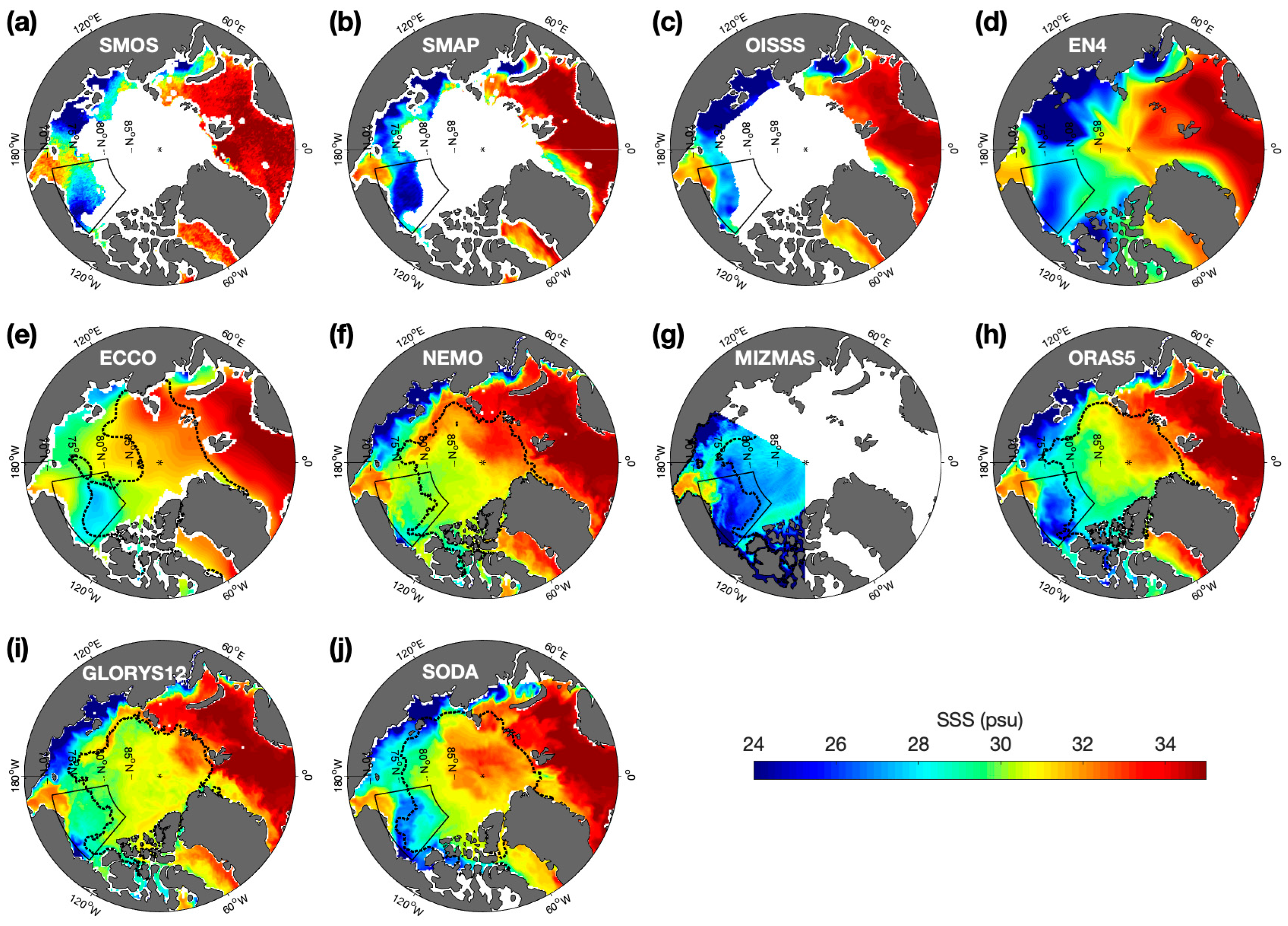
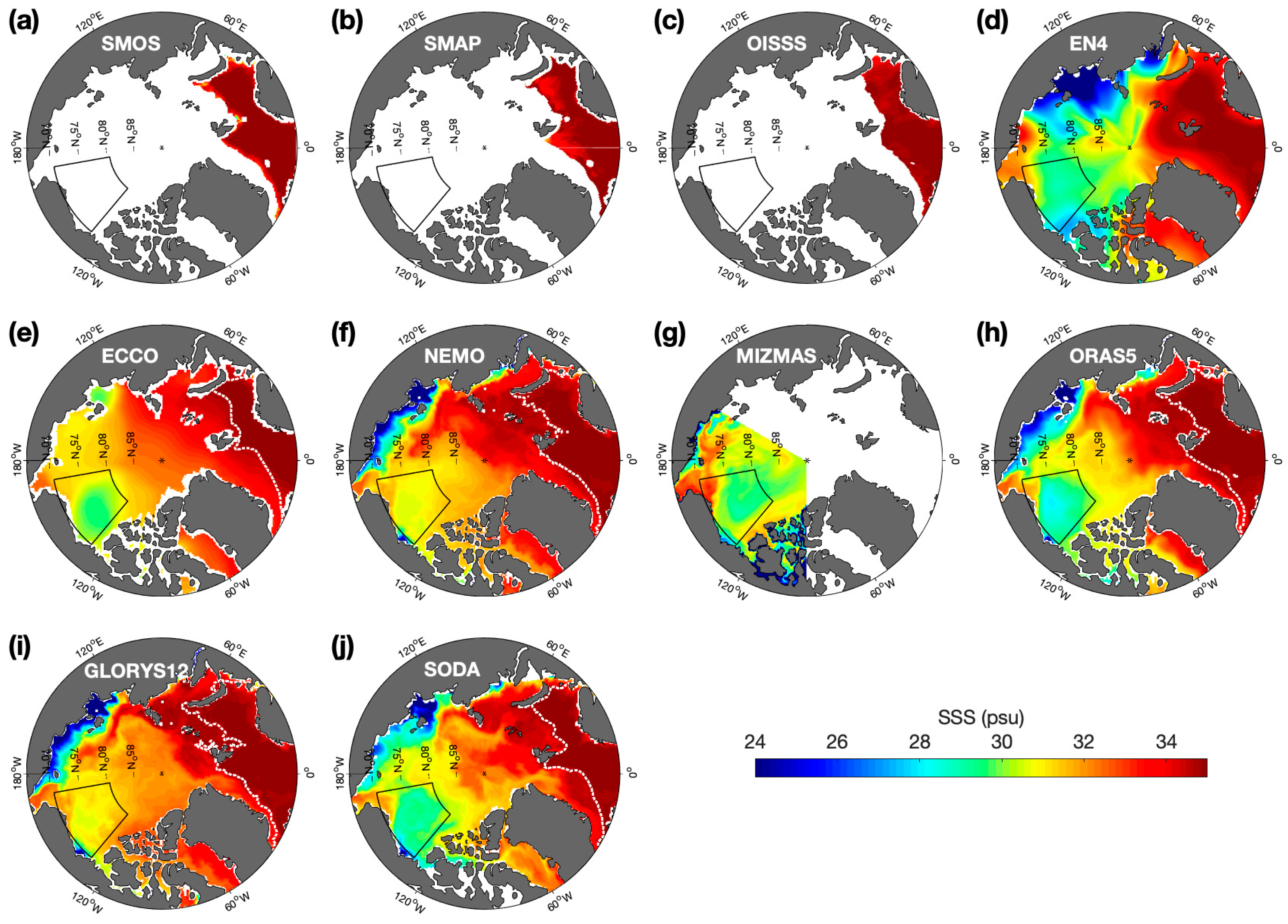
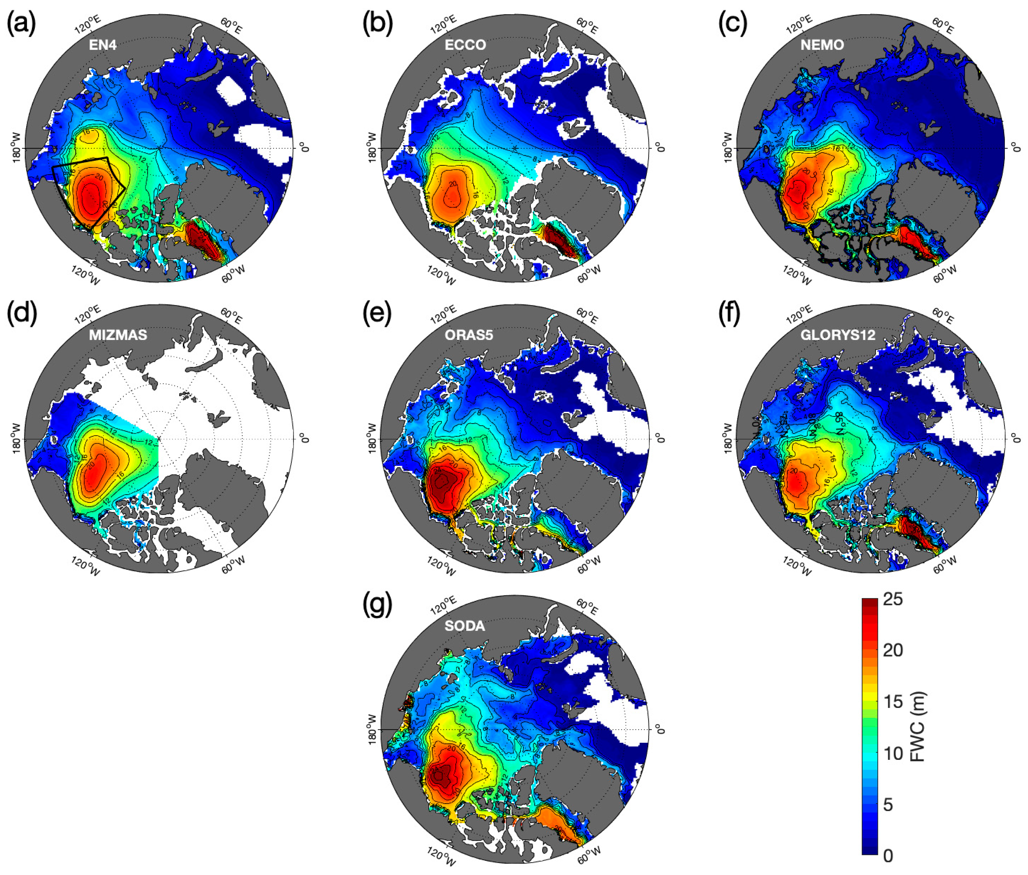
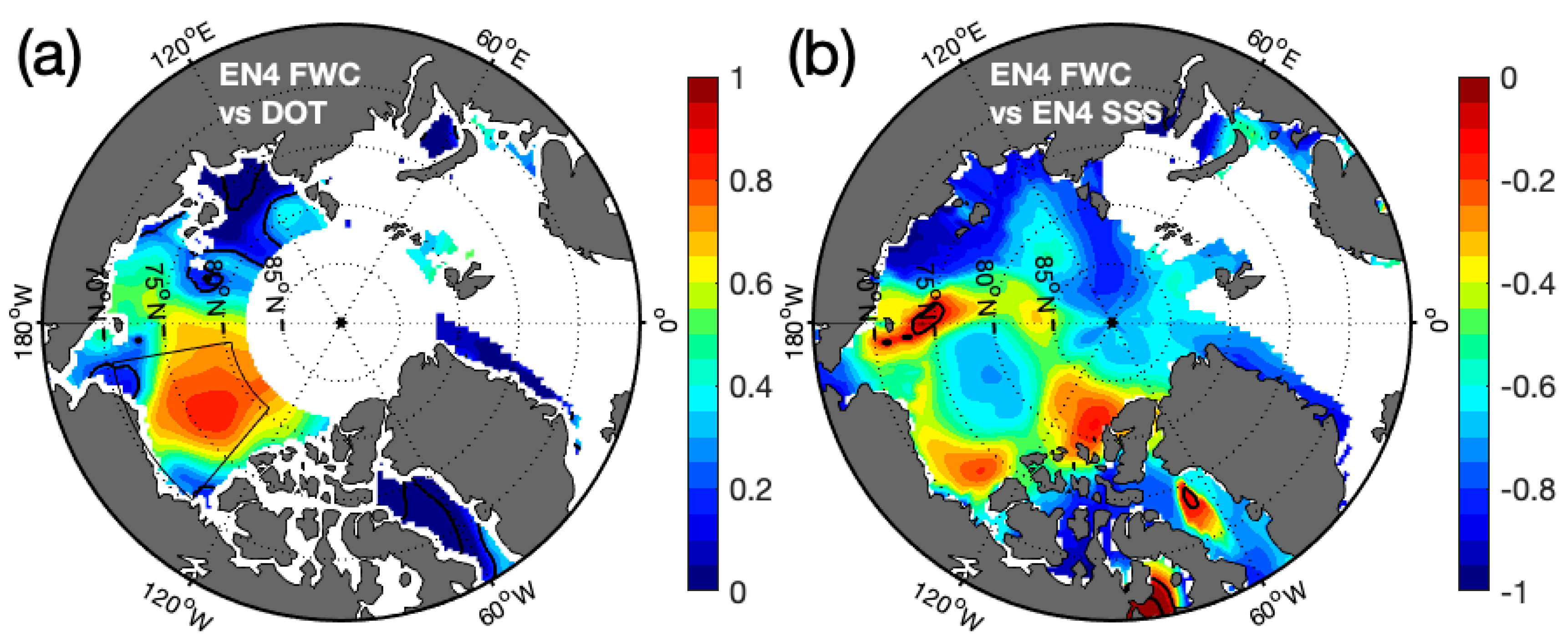
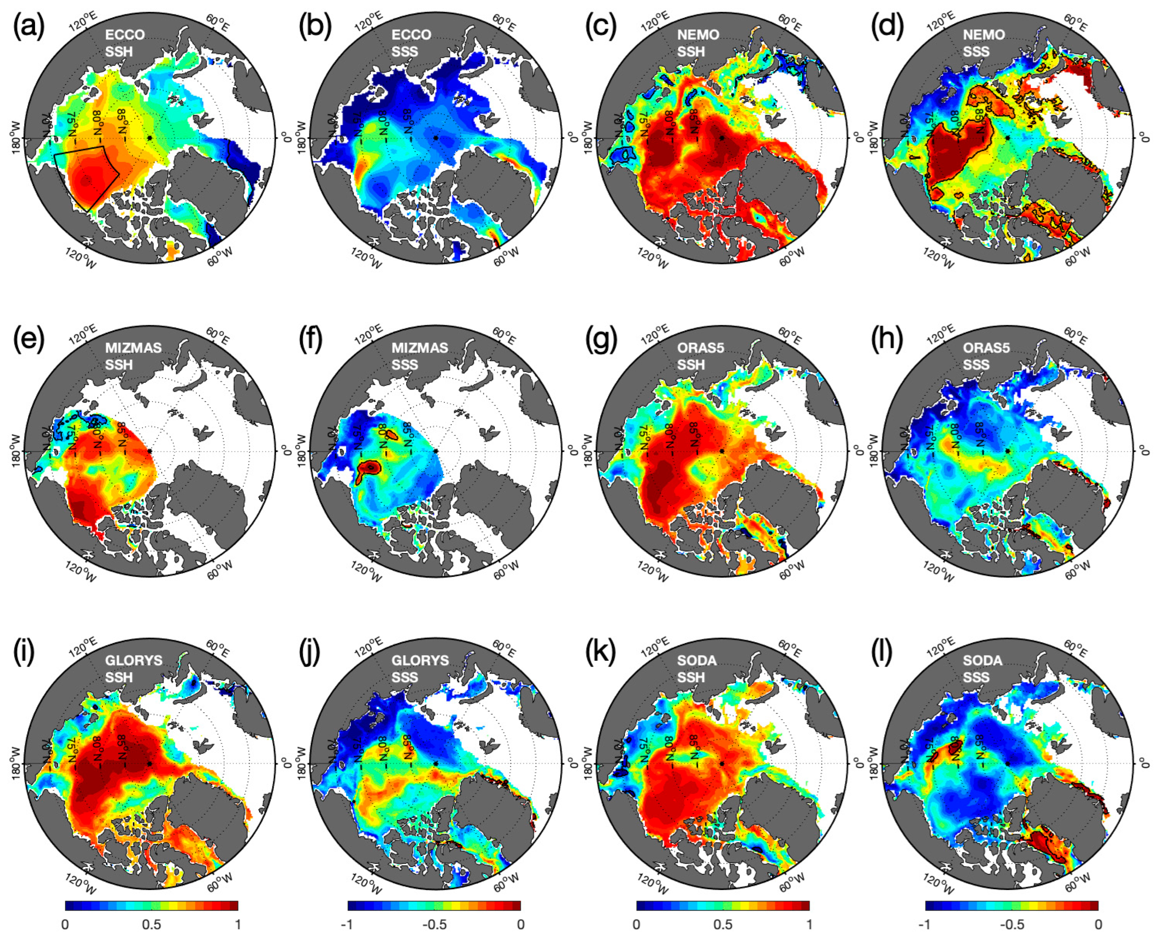
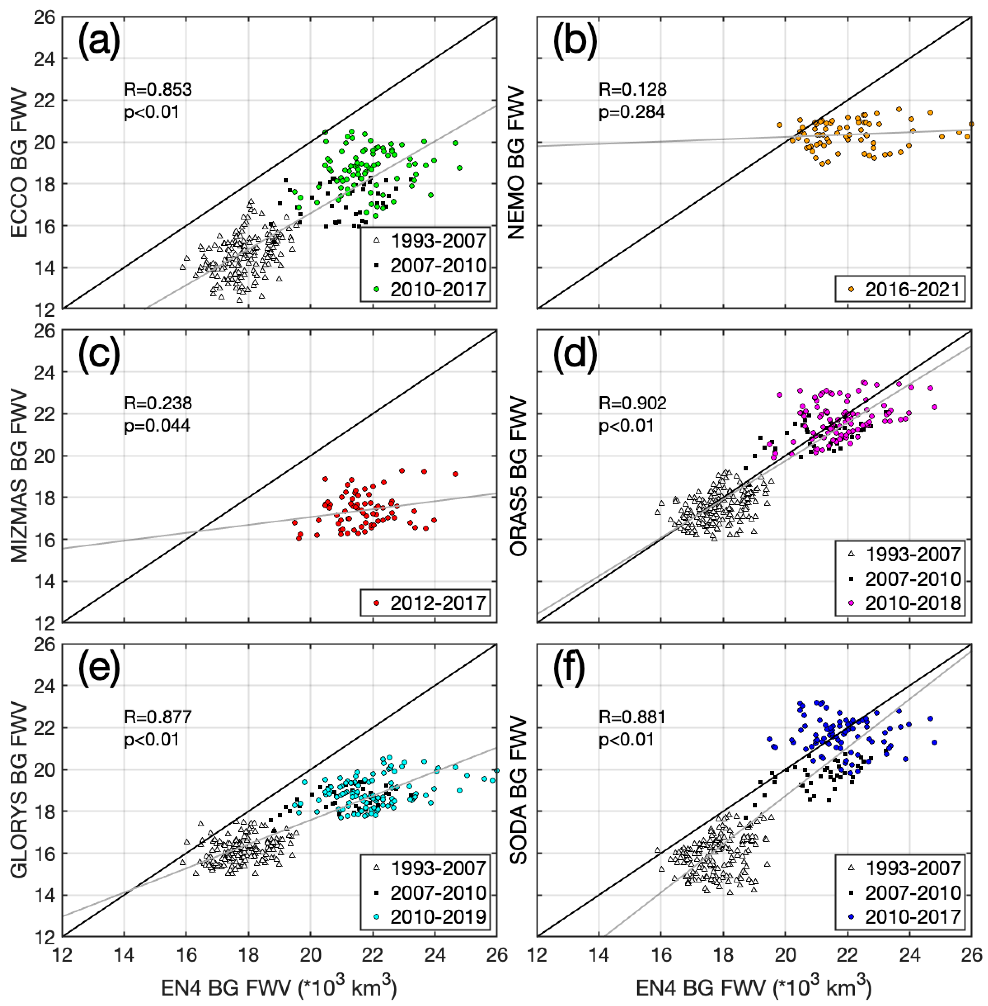
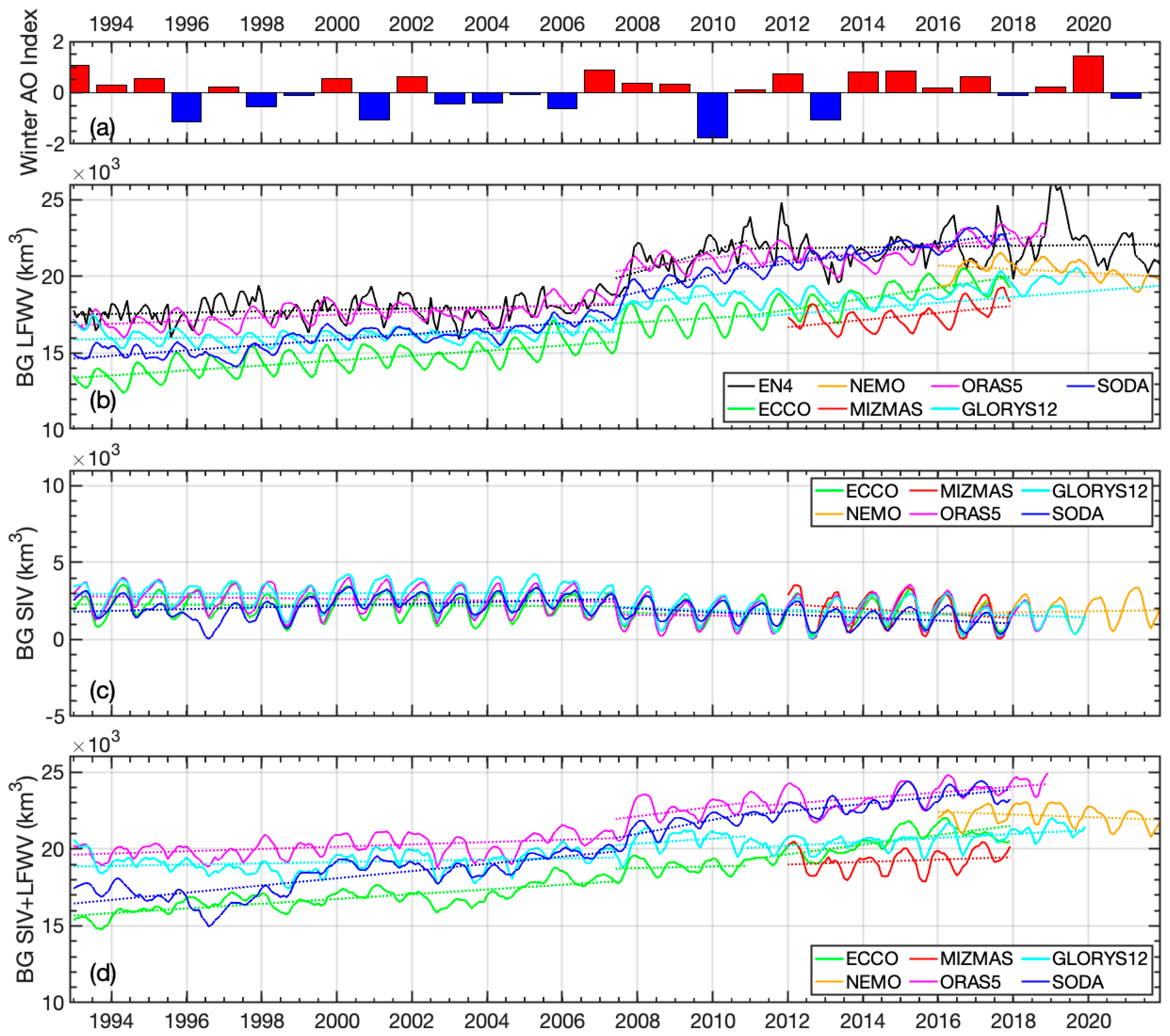
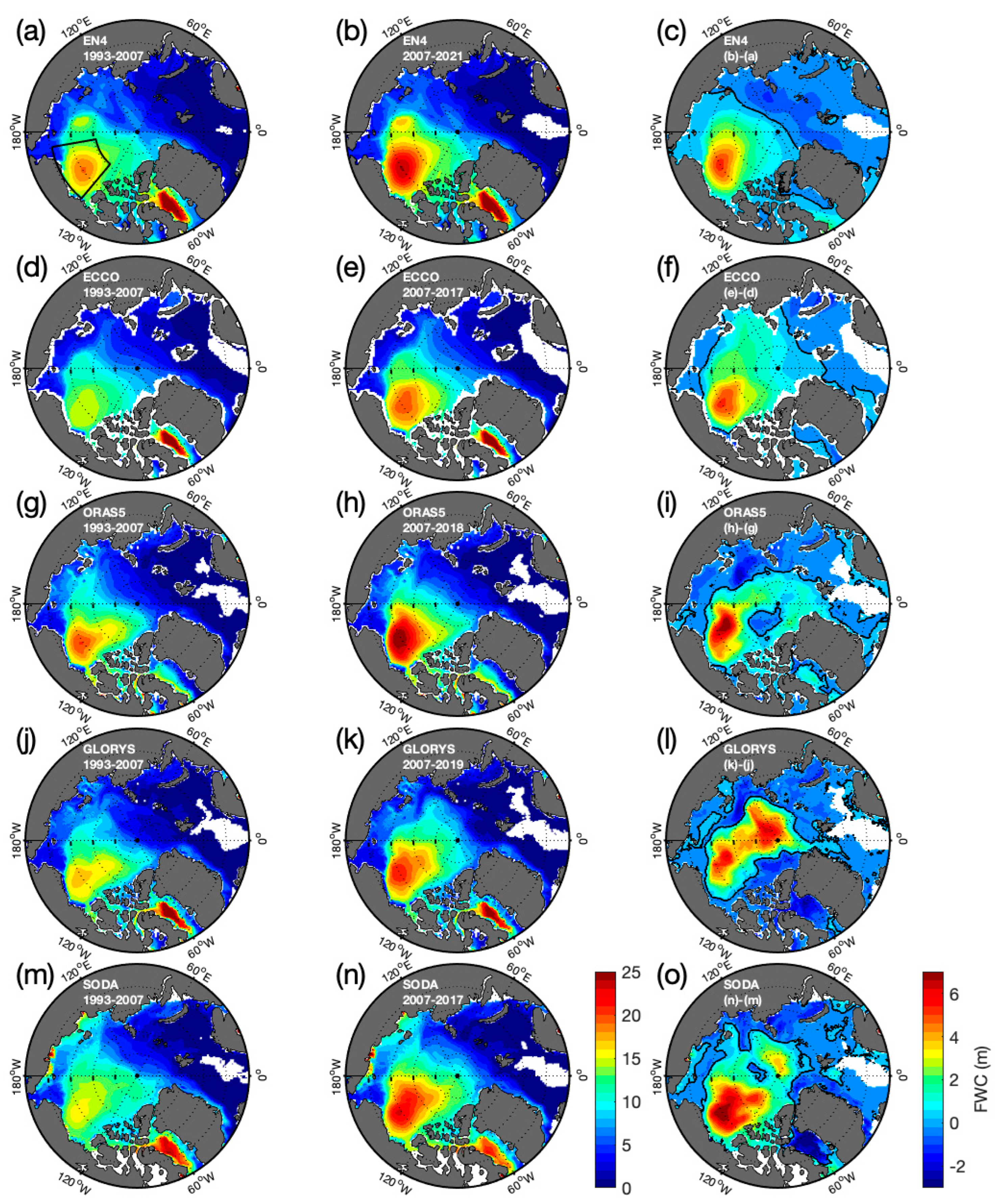
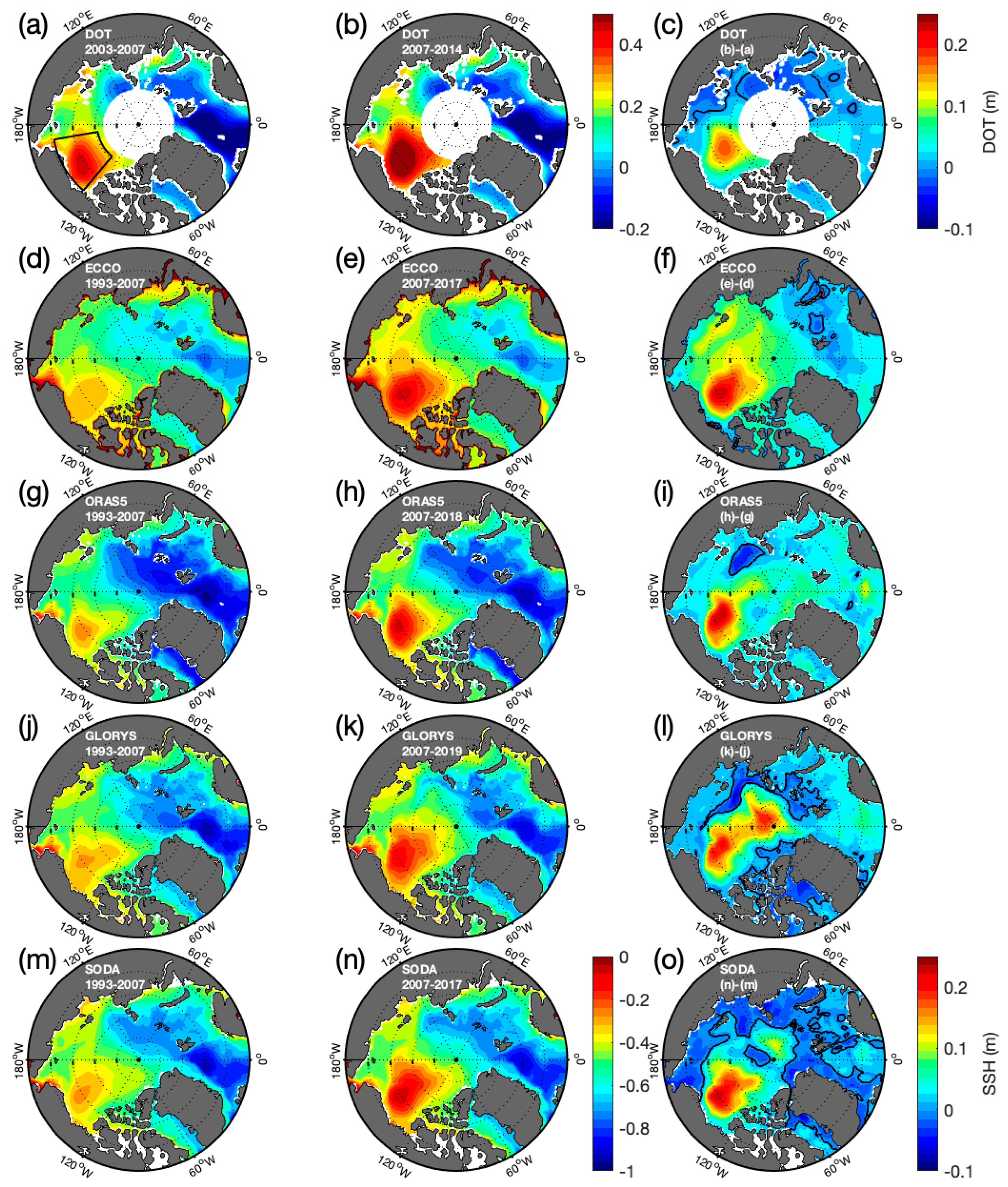
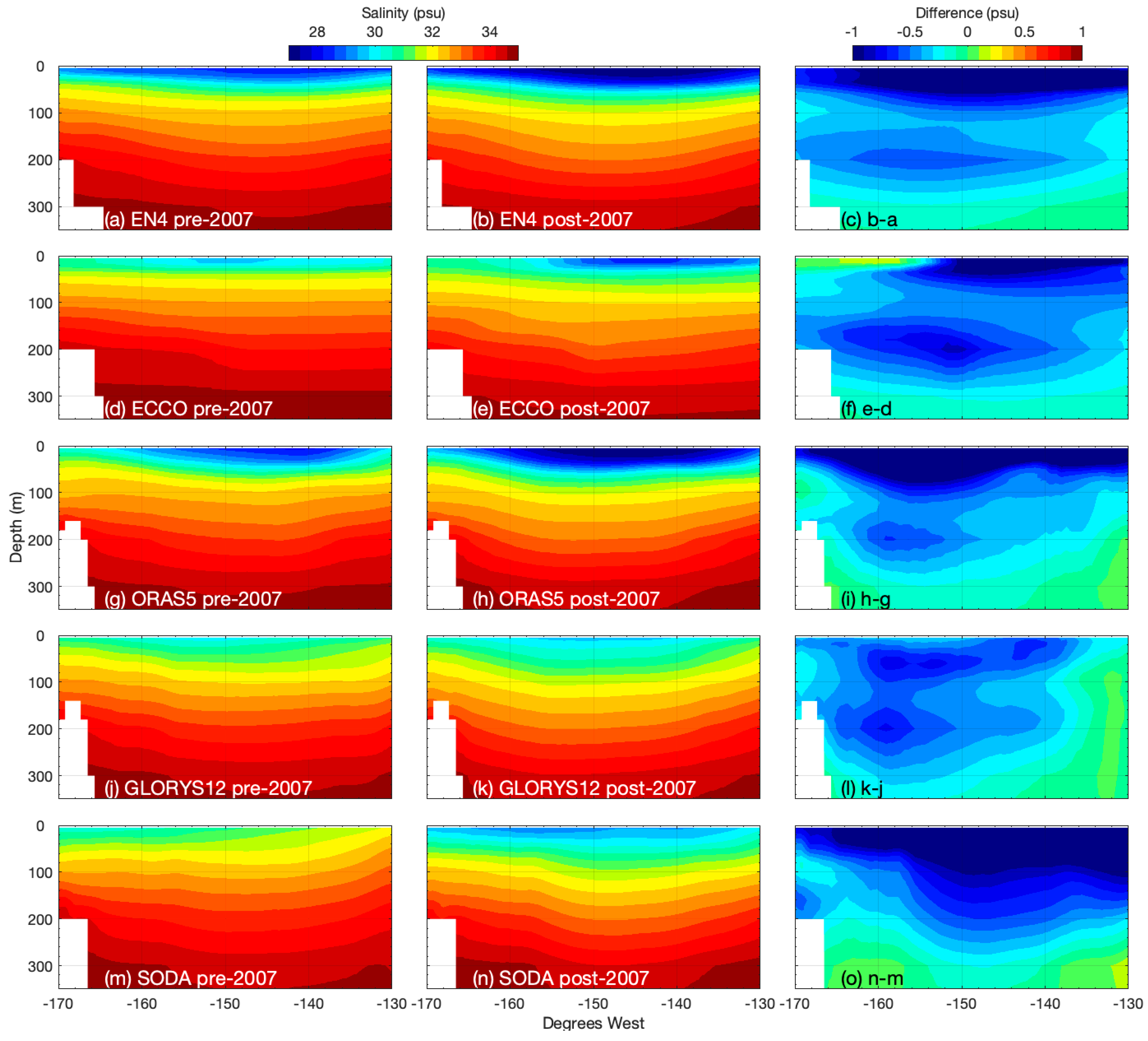
Table 1.
Summary of descriptions for the model and reanalysis products used in this study.
| Product | ECCO | NEMO | MIZMAS | ORAS5 | GLORYS12 | SODA3 |
|---|---|---|---|---|---|---|
| Version | Version 4, release 4 | Version 3.1 | Version 1 | Version 5 | Version 1 Level 4 | Version 3.12 |
| Origin | NASA | ECMWF | APL/PSC | ECMWF/ICDC | CMEMS | UofMD |
| Horizontal Resolution | 1-1/5°; LLC90 grid | 1/12° gridded (ORCA) | 1/5° gridded | 1/4° gridded | 1/12° gridded | 1/2° gridded |
| Temporal Resolution | Daily and monthly; January 1992–December 2017 | Daily; January 2016–December 2021 | Daily; January 2012–December 2017 | Monthly; January 1979–December 2018 | Daily; January 1993–December 2019 | Monthly; January 1980–December 2017 |
| Vertical Layers | 50; 5 m–5.9 km | 50; 0.5 m–5.7 km | 40; 0.5 m–4.3 km | 75; 0.5 m–5.9 km | 50; 0.5 m–5.7 km | 50; 5 m–5.4 km |
| Ocean and Ice Data | Aquarius SSS constrained; Argo floats, WOA09 CTDs, APB gliders, ITPs, moorings, Fekete et al., 2002 river discharge assimilated | Altimeter data, CMEMS in situ temperature and salinity vertical profiles, SIC, SLA, satellite SST, Dai et al., 2009 river discharge assimilated | Parallel Ocean Program model + TED sea ice model; polar profiling floats, ITPs, autonomous glider data assimilated | NEMOv3.4 + LIM2 sea ice model; HadISST2 SST, OSTIA SIC, EN4 in situ, AVISO DT2014 SLA assimilated | NEMOv3.4 and ORCA12; CMEMS SLA, AVHRR SST data, CORA in situ database, Dai et al., 2009 river discharge assimilated | Modular Ocean Model v5.1 + Sea Ice Simulator, WOD13 and ICOADS v5r2, Dai et al., 2009 river discharge assimilated |
| Atmospheric Data | ECMWF ERA-Interim | ECMWF forecast, bulk CORE formulas | NCEP CFSv2, NCAR reanalysis data | ERA-Interim (1979–2014), ECMWF NWP (2015–2018), WAVE forcing | ERA-Interim | JRA-55DO atmospheric reanalysis with CORE4 bulk formula |
Disclaimer/Publisher’s Note: The statements, opinions and data contained in all publications are solely those of the individual author(s) and contributor(s) and not of MDPI and/or the editor(s). MDPI and/or the editor(s) disclaim responsibility for any injury to people or property resulting from any ideas, methods, instructions or products referred to in the content. |
© 2023 by the authors. Licensee MDPI, Basel, Switzerland. This article is an open access article distributed under the terms and conditions of the Creative Commons Attribution (CC BY) license (https://creativecommons.org/licenses/by/4.0/).
Share and Cite
MDPI and ACS Style
Hoffman, E.L.; Subrahmanyam, B.; Trott, C.B.; Hall, S.B. Comparison of Freshwater Content and Variability in the Arctic Ocean Using Observations and Model Simulations. Remote Sens. 2023, 15, 3715. https://doi.org/10.3390/rs15153715
AMA Style
Hoffman EL, Subrahmanyam B, Trott CB, Hall SB. Comparison of Freshwater Content and Variability in the Arctic Ocean Using Observations and Model Simulations. Remote Sensing. 2023; 15(15):3715. https://doi.org/10.3390/rs15153715
Chicago/Turabian StyleHoffman, Emma L., Bulusu Subrahmanyam, Corinne B. Trott, and Sarah B. Hall. 2023. "Comparison of Freshwater Content and Variability in the Arctic Ocean Using Observations and Model Simulations" Remote Sensing 15, no. 15: 3715. https://doi.org/10.3390/rs15153715
Note that from the first issue of 2016, this journal uses article numbers instead of page numbers. See further details here.