
Uncertainty Evaluation on Temperature Detection of Middle Atmosphere by Rayleigh Lidar
 , ,
, ,
Abstract
:1. Introduction
2. Atmospheric Temperature Measurement Models
2.1. Lidar Equation
2.2. Chanin-Hauchecorne Method for Atmospheric Temperature Retrieval
3. Atmospheric Temperature Uncertainty Evaluation with Simulation Data
3.1. Temperature Uncertainty Evaluation by GUM
3.1.1. The Law of Uncertainty Propagation
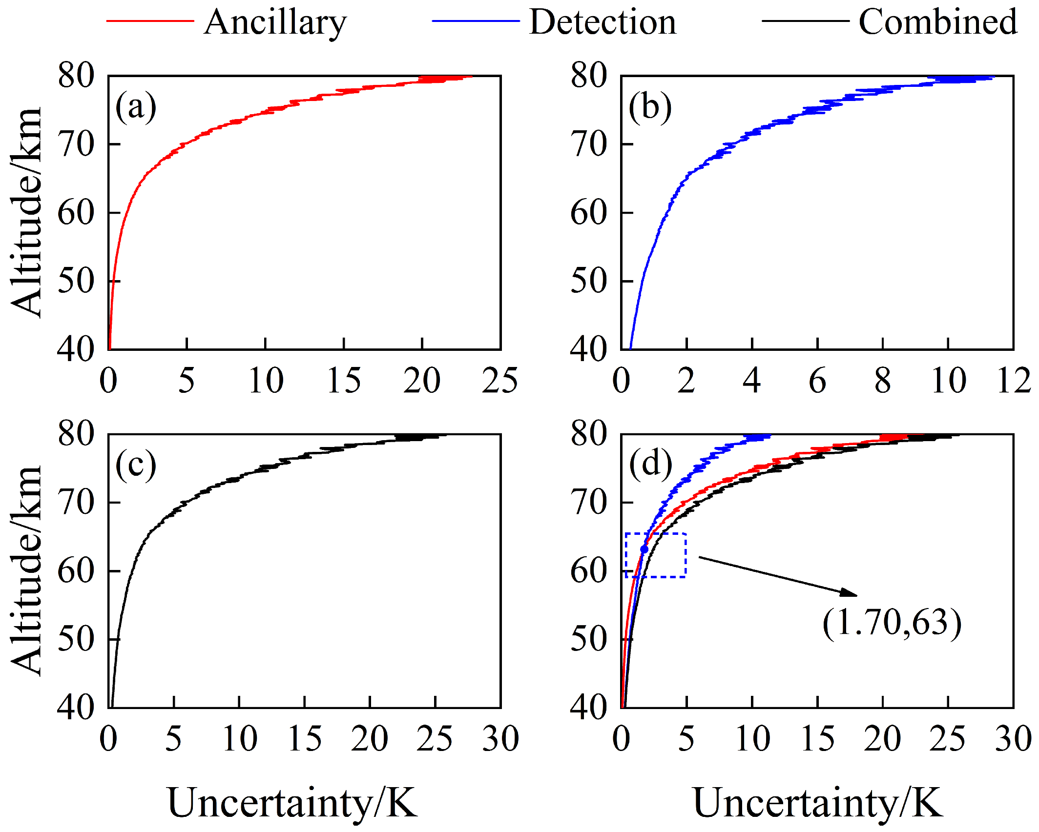
3.1.2. Temperature Uncertainty Owing to Auxiliary Temperature Uncertainty
3.1.3. Temperature Uncertainty Owing to Detection Noise
3.1.4. Combined Standard Uncertainty
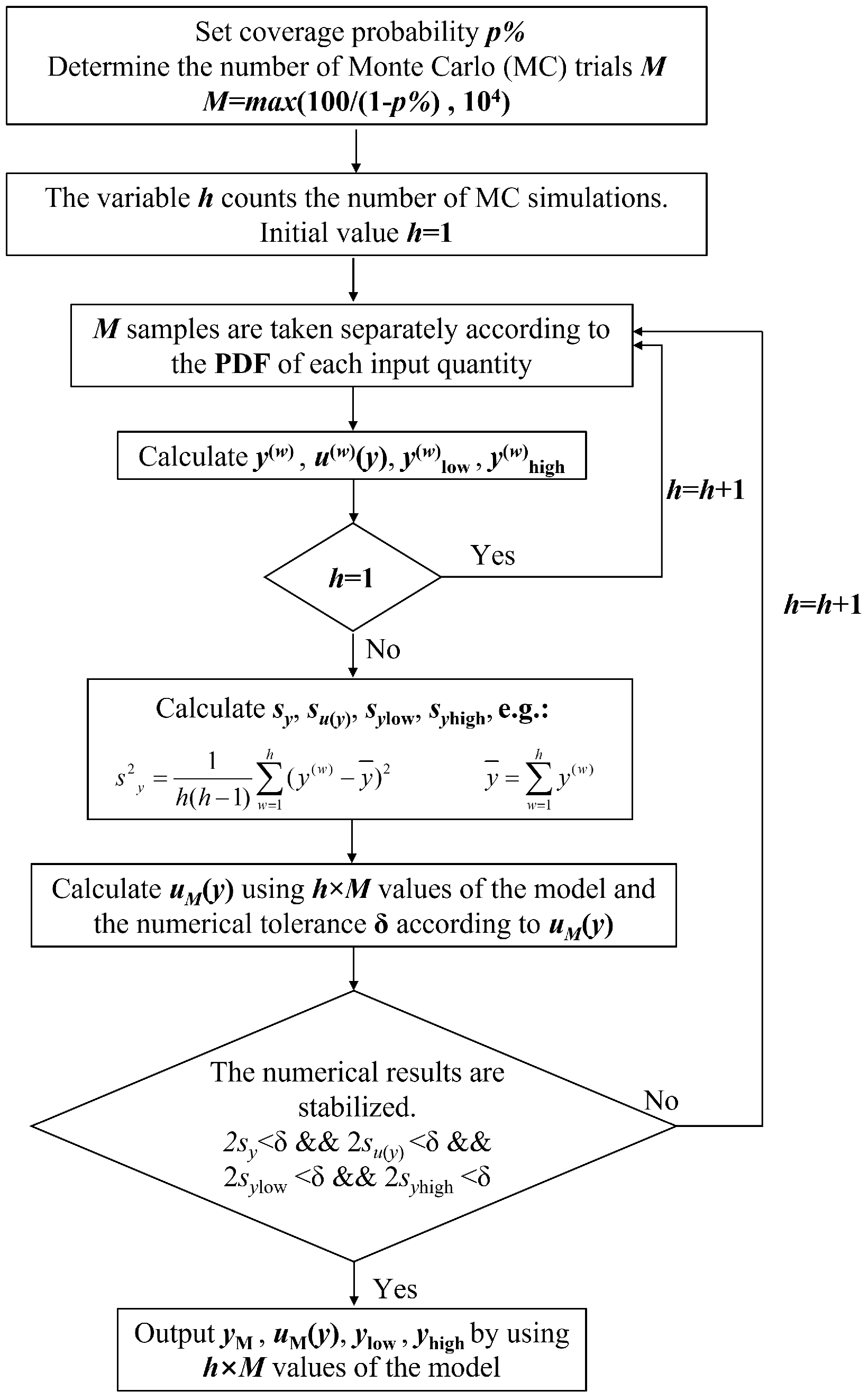
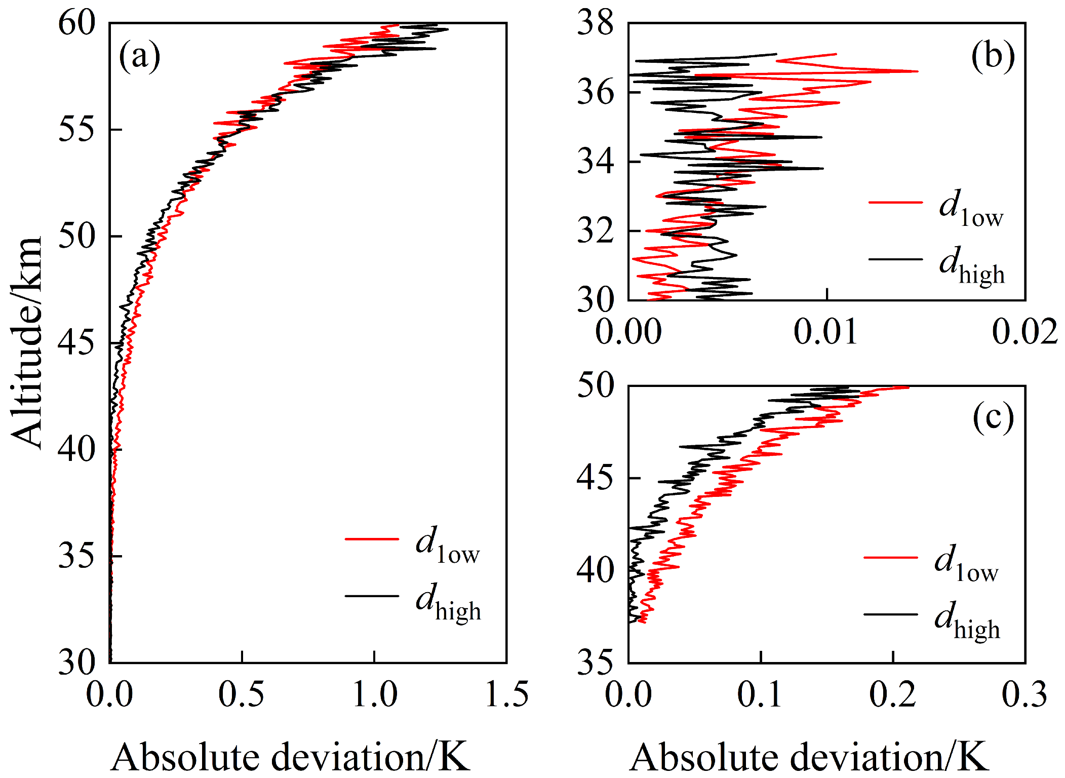
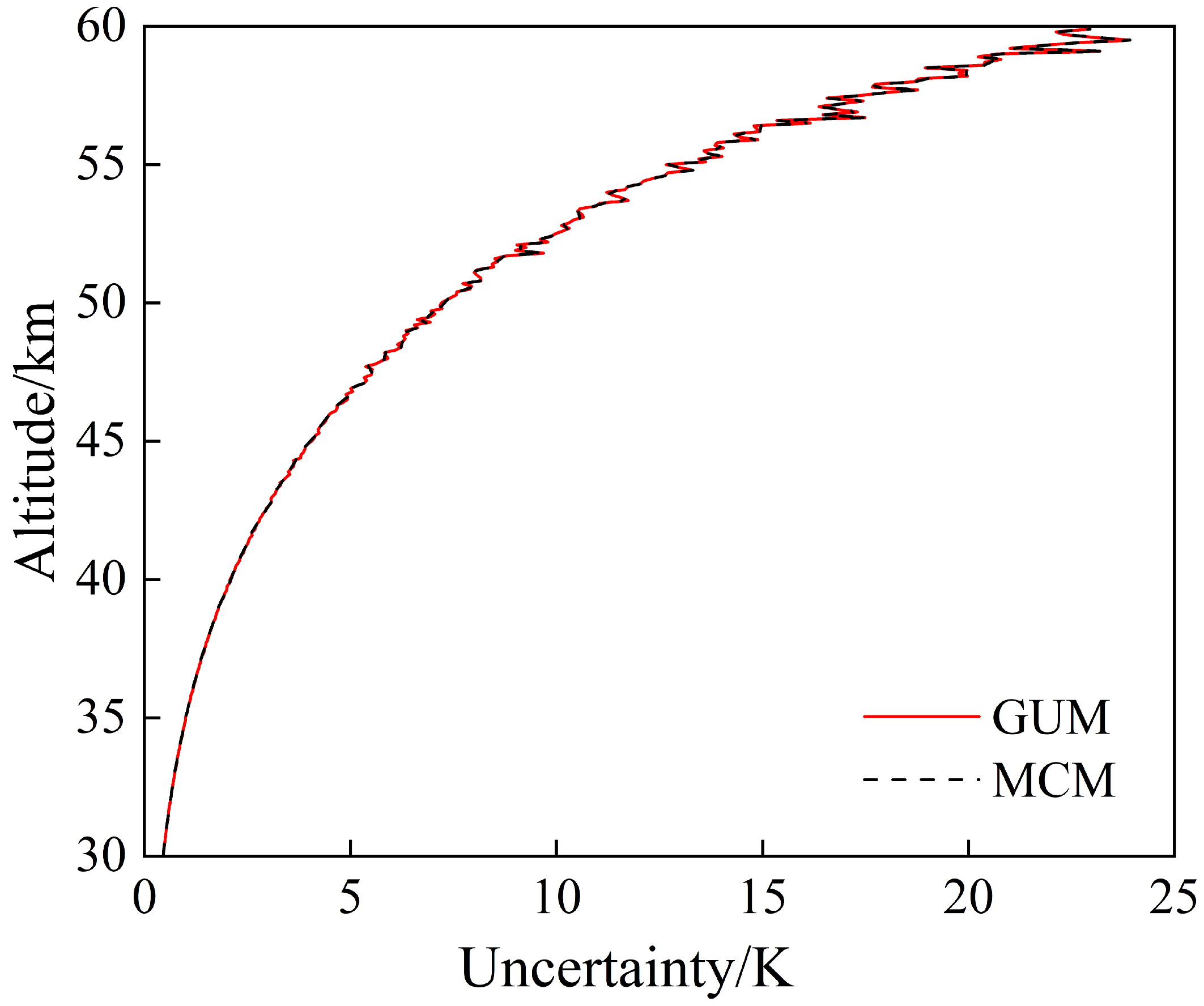
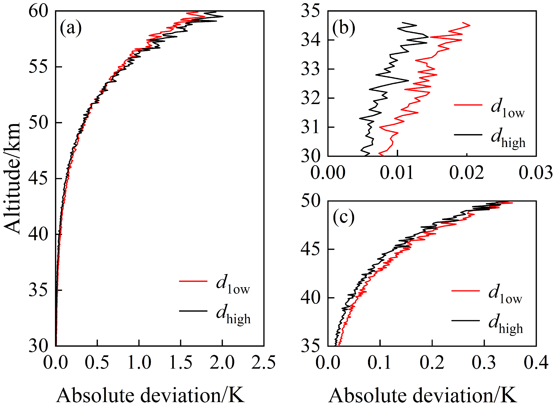
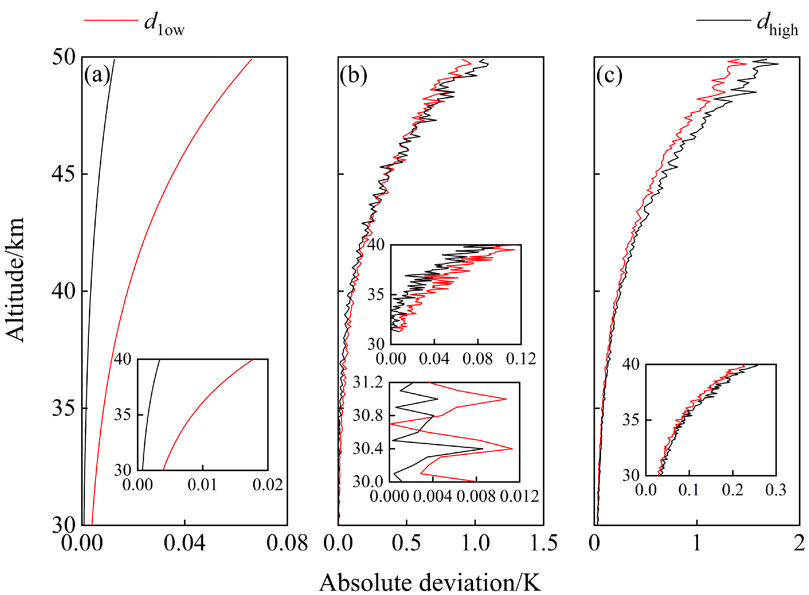
3.2. Temperature Uncertainty Evaluation by MCM
3.2.1. Temperature Uncertainty Owing to Auxiliary Temperature Uncertainty
3.2.2. Temperature Uncertainty Owing to Detection Noise
3.2.3. Combined Standard Uncertainty
4. Calculation Example of the Temperature Uncertainty with Measured Data
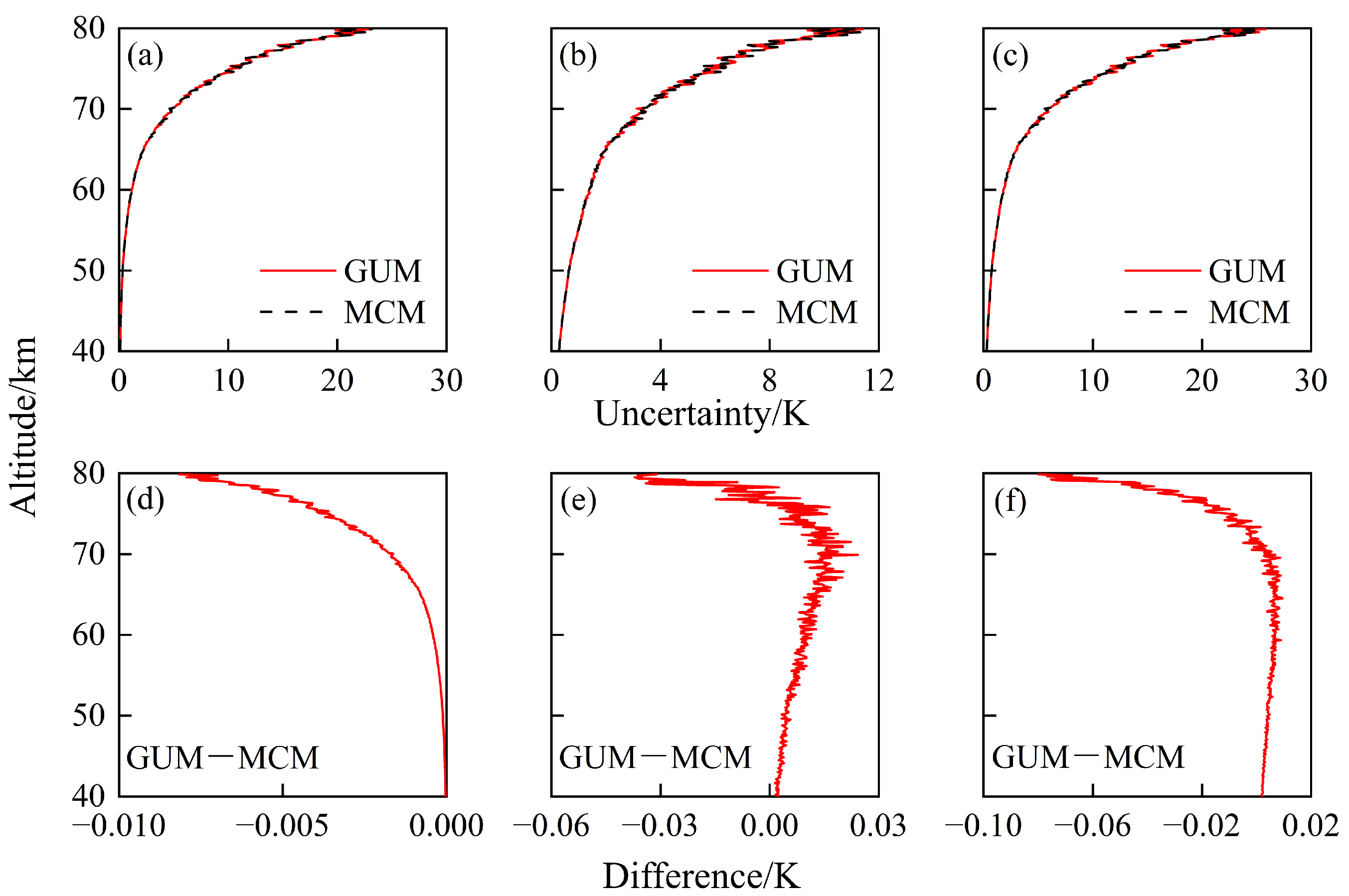
4.1. Temperature Uncertainty Evaluation by GUM
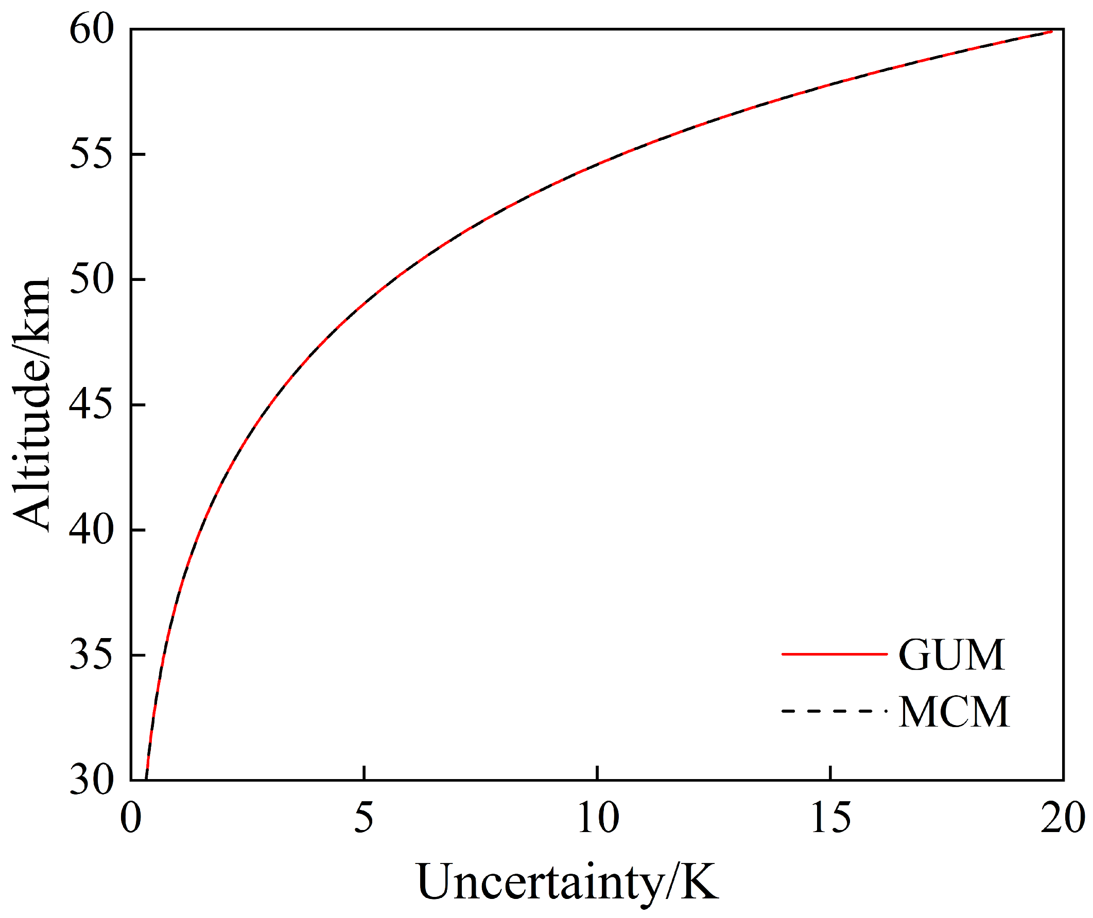
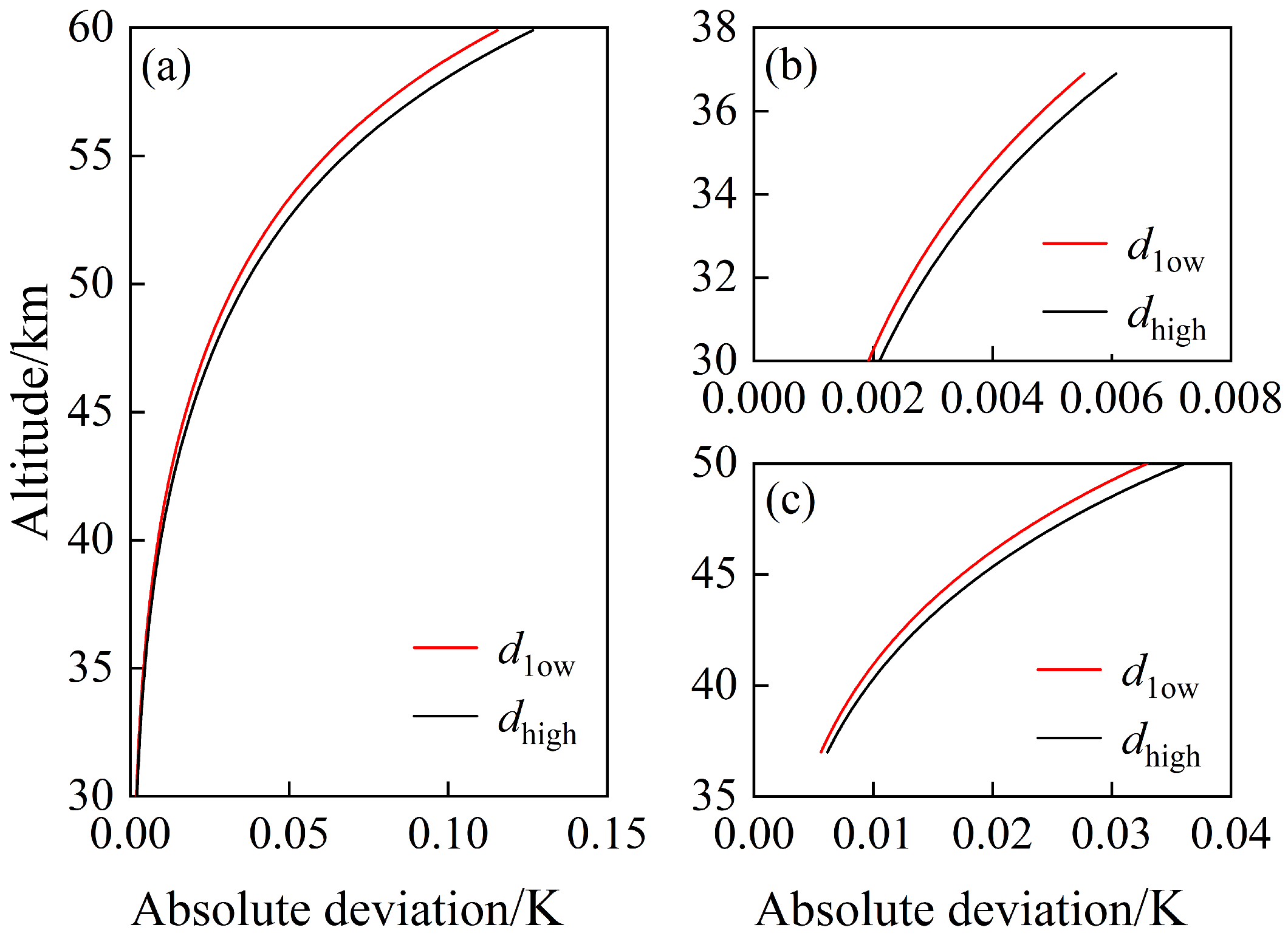
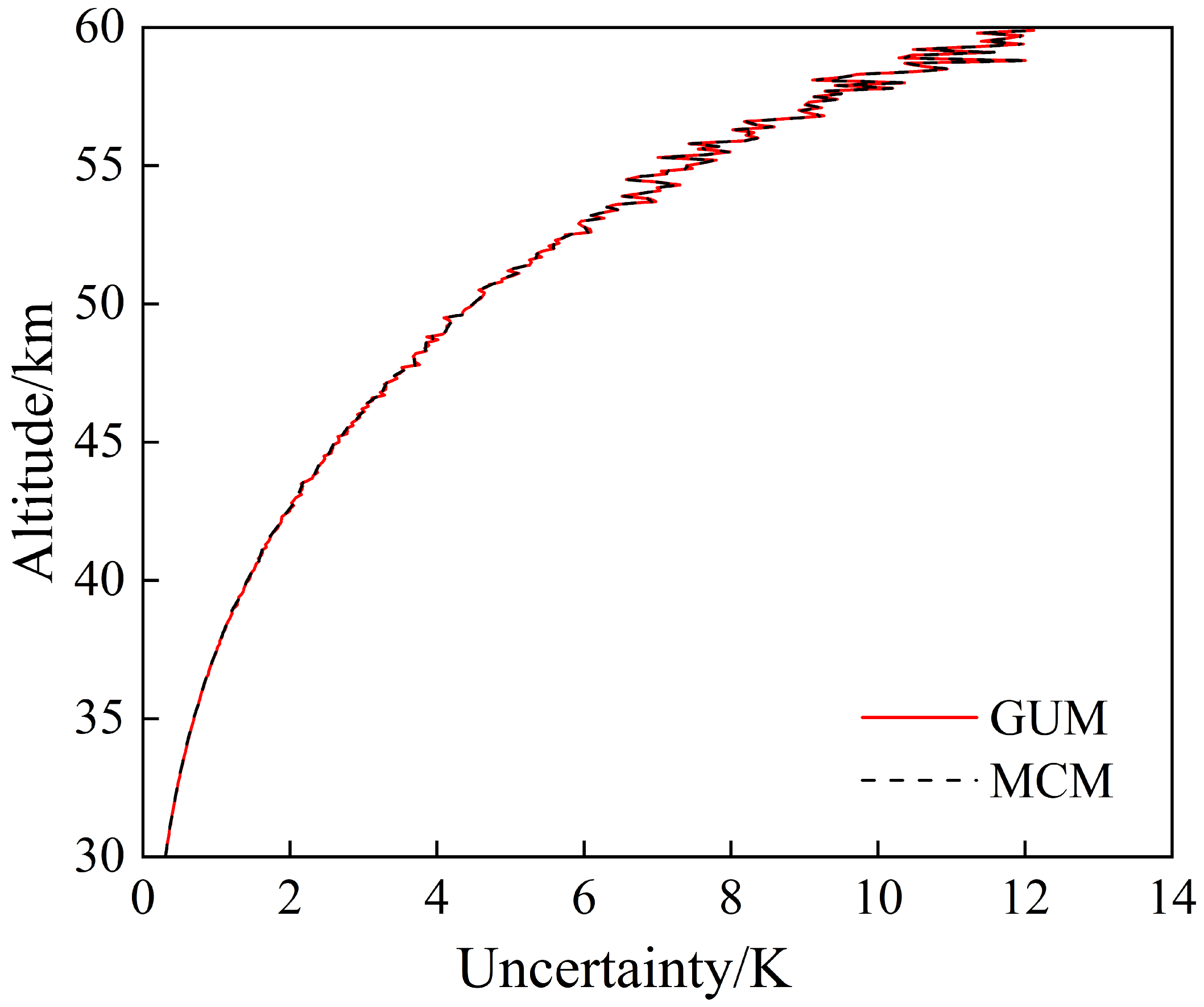
4.2. Comparison between GUM and MCM
5. Conclusions
Author Contributions
Funding
Data Availability Statement
Conflicts of Interest
References
- Deng, P. Observing and Studying the near Space Atmosphere by Ground-Based Lidar. Ph.D. Thesis, University of Science and Technology of China, Hefei, China, 2018. [Google Scholar]
- Schmidlin, F. Temperature inversions near 75 km. Geophys. Res. Lett. 1976, 3, 173–176. [Google Scholar] [CrossRef]
- Sharma, S.; Kumar, P.; Vaishnav, R.; Jethva, C.; Bencherif, H. Evaluation of Inter-Hemispheric Characteristics of the Tropopause–Stratopause–Mesopause Over Sub-Tropical Regions. Pure Appl. Geophys. 2018, 175, 1123–1137. [Google Scholar] [CrossRef]
- Kaifler, B.; Kaifler, N. A Compact Rayleigh Autonomous Lidar (CORAL) for the middle atmosphere. Atmos. Meas. Tech. 2021, 14, 1715–1732. [Google Scholar] [CrossRef]
- Wing, R.; Martic, M.; Triplett, C.; Hauchecorne, A.; Porteneuve, J.; Keckhut, P.; Courcoux, Y.; Yung, L.; Retailleau, P.; Cocuron, D. Gravity Wave Breaking Associated with Mesospheric Inversion Layers as Measured by the Ship-Borne BEM Monge Lidar and ICON-MIGHTI. Atmosphere 2021, 12, 1386. [Google Scholar] [CrossRef]
- Rapp, M.; Kaifler, B.; Dörnbrack, A.; Gisinger, S.; Mixa, T.; Reichert, R.; Kaifler, N.; Knobloch, S.; Eckert, R.; Wildmann, N.; et al. SOUTHTRAC-GW: An airborne field campaign to explore gravity wave dynamics at the world’s strongest hotspot. Bull. Am. Meteorol. Soc. 2021, 102, E871–E893. [Google Scholar] [CrossRef]
- Kaifler, B.; Rempel, D.; Roßi, P.; Büdenbender, C.; Kaifler, N.; Baturkin, V. A technical description of the Balloon Lidar Experiment (BOLIDE). Atmos. Meas. Tech. 2020, 13, 5681–5695. [Google Scholar] [CrossRef]
- De Mazière, M.; Thompson, A.M.; Kurylo, M.J.; Wild, J.D.; Bernhard, G.; Blumenstock, T.; Braathen, G.O.; Hannigan, J.W.; Lambert, J.C.; Leblanc, T.; et al. The Network for the Detection of Atmospheric Composition Change (NDACC): History, status and perspectives. Atmos. Chem. Phys. 2018, 18, 4935–4964. [Google Scholar] [CrossRef] [Green Version]
- Hauchecorne, A.; Chanin, M.L. Density and temperature profiles obtained by lidar between 35 and 70 km. Geophys. Res. Lett. 1980, 7, 565–568. [Google Scholar] [CrossRef]
- Deng, P.; Zhang, T.S.; Chen, W.; Liu, Y. Lidar measurement for atmospheric density and temperature in middle atmosphere over Hefei. Infrared Laser Eng. 2017, 46, 70–75. [Google Scholar]
- David, C.; Haefele, A.; Keckhut, P.; Marchand, M.; Jumelet, J.; Leblanc, T.; Cénac, C.; Laqui, C.; Porteneuve, J.; Haeffelin, M.; et al. Evaluation of stratospheric ozone, temperature, and aerosol profiles from the LOANA lidar in Antarctica. Polar Sci. 2012, 6, 209–225. [Google Scholar] [CrossRef]
- Liu, X. The Algorithm for Retrieval of Middle Atmospheric Temperature Using Rayleigh Lidar. Master’s Thesis, National Space Science Center, The Chinese Academy of Sciences, Beijing, China, 2018. [Google Scholar]
- Gu, Y.Y.; Gardner, C.S.; Castleberg, P.A.; Papen, G.C.; Kelley, M.C. Validation of the Lidar In-Space Technology Experiment: Stratospheric temperature and aerosol measurements. Appl. Opt. 1997, 36, 5148–5157. [Google Scholar] [CrossRef] [PubMed]
- Chen, W.; Tsao, C.; Nee, J. Rayleigh lidar temperature measurements in the upper troposphere and lower stratosphere. J. Atmos. Sol. Terr. Phys. 2004, 66, 39–49. [Google Scholar] [CrossRef]
- Herron, J.P. Rayleigh-Scatter Lidar Observations at USU’s Atmospheric Lidar Observatory (Logan, Utah): Temperature Climatology, Temperature Comparisons with MSIS, and Noctilucent Clouds. Ph.D. Thesis, Utah State University, Logan, UT, USA, 2007. [Google Scholar]
- Sica, R.; Sargoytchev, S.; Argall, P.; Borra, E.; Girard, L.; Sparrow, C.; Flatt, S. Lidar measurements taken with a large-aperture liquid mirror. 1. Rayleigh-scatter system. Appl. Opt. 1995, 34, 6925–6936. [Google Scholar] [CrossRef] [PubMed]
- Wu, Y.H.; Hu, H.L.; Hu, S.X. Temperature measurement with Rayleigh scattering lidar in the mid and upper stratosphere. Chin. J. Lasers 2001, 28, 137–140. [Google Scholar]
- Chang, Q.H. By Rayleigh Lidar Observing and Studying the Middle Atmosphere over Wuhan. Ph.D. Thesis, Wuhan Institute of Physics and Mathematics, The Chinese Academy of Science, Wuhan, China, 2005. [Google Scholar]
- Knobloch, S.; Kaifler, B.; Rapp, M. Estimating the uncertainty of middle-atmospheric temperatures retrieved from airborne Rayleigh lidar measurements. Atmos. Meas. Tech. Discuss. 2022. preprint. [Google Scholar] [CrossRef]
- Chen, A.; Chen, C. Comparison of GUM and Monte Carlo methods for evaluating measurement uncertainty of perspiration measurement systems. Measurement 2016, 87, 27–37. [Google Scholar] [CrossRef]
- Chen, Y.; Li, X.; Huang, L.; Wang, X.; Liu, C.; Zhao, F.; Hua, Y.; Feng, P. GUM method for evaluation of measurement uncertainty: BPL long wave time service monitoring. Measurement 2022, 189, 110459. [Google Scholar] [CrossRef]
- Ferreira, R.; Silva, B.; Teixeira, G.; Andrade, R.; Porto, M. Uncertainty analysis applied to electrical components diagnosis by infrared thermography. Measurement 2019, 132, 263–271. [Google Scholar] [CrossRef]
- Leblanc, T.; Sica, R.J.; van Gijsel, J.A.; Haefele, A.; Payen, G.; Liberti, G. Proposed standardized definitions for vertical resolution and uncertainty in the NDACC lidar ozone and temperature algorithms–Part 3: Temperature uncertainty budget. Atmos. Meas. Tech. 2016, 9, 4079–4101. [Google Scholar] [CrossRef] [Green Version]
- JCGM. Evaluation of measurement data—Guide to the expression of uncertainty in measurement. Int. Bur. Weight. Meas. BIPM 2008, 100, 1–116. [Google Scholar]
- JCGM. Evaluation of Measurement Data-Supplement 1 to the “Guide to the Expression of Uncertainty in Measurement”—Propagation of Distributions Using a Monte Carlo Method; International Bureau of Weights and Measures (BIPM): Sèvres, France, 2008. [Google Scholar]
- Picone, J.; Hedin, A.; Drob, D.P.; Aikin, A. NRLMSISE-00 empirical model of the atmosphere: Statistical comparisons and scientific issues. J. Geophys. Res. 2002, 107, SIA-15. [Google Scholar] [CrossRef]
- Donovan, D.; Whiteway, J.; Carswell, A.I. Correction for nonlinear photon-counting effects in lidar systems. Appl. Opt. 1993, 32, 6742–6753. [Google Scholar] [CrossRef] [PubMed]
- Khanna, J.; Bandoro, J.; Sica, R.; McElroy, C.T. New technique for retrieval of atmospheric temperature profiles from Rayleigh-scatter lidar measurements using nonlinear inversion. Appl. Opt. 2012, 51, 7945–7952. [Google Scholar] [CrossRef] [PubMed]
- Leblanc, T.; Sica, R.J.; van Gijsel, E.J.A.; Godin-Beekmann, S.; Haefele, A.; Trickl, T.; Payen, G.; Liberti, G. Standardized Definition and Reporting of Vertical Resolution and Uncertainty in the NDACC Lidar Ozone and Temperature Algorithms, ISSI Team on NDACC Lidar Algorithms Report. Available online: http://www.issibern.ch/teams/ndacc/ISSI_Team_Report.htm (accessed on 2 May 2023).


| System Parameter | Value |
|---|---|
| Laser wavelength/nm | 532 |
| Repetition frequency/Hz | 50 |
| Pulse energy/mJ | 40 |
| System efficiency | 0.191 |
| Range resolution/m | 100 |
| Receiver diameter/m | 0.35 |
| Field of view/rad | 165 |
| Dark counts | 50 |
| Filter bandwidth/nm | 0.25 |
| Lidar-site altitude/km | 20 |
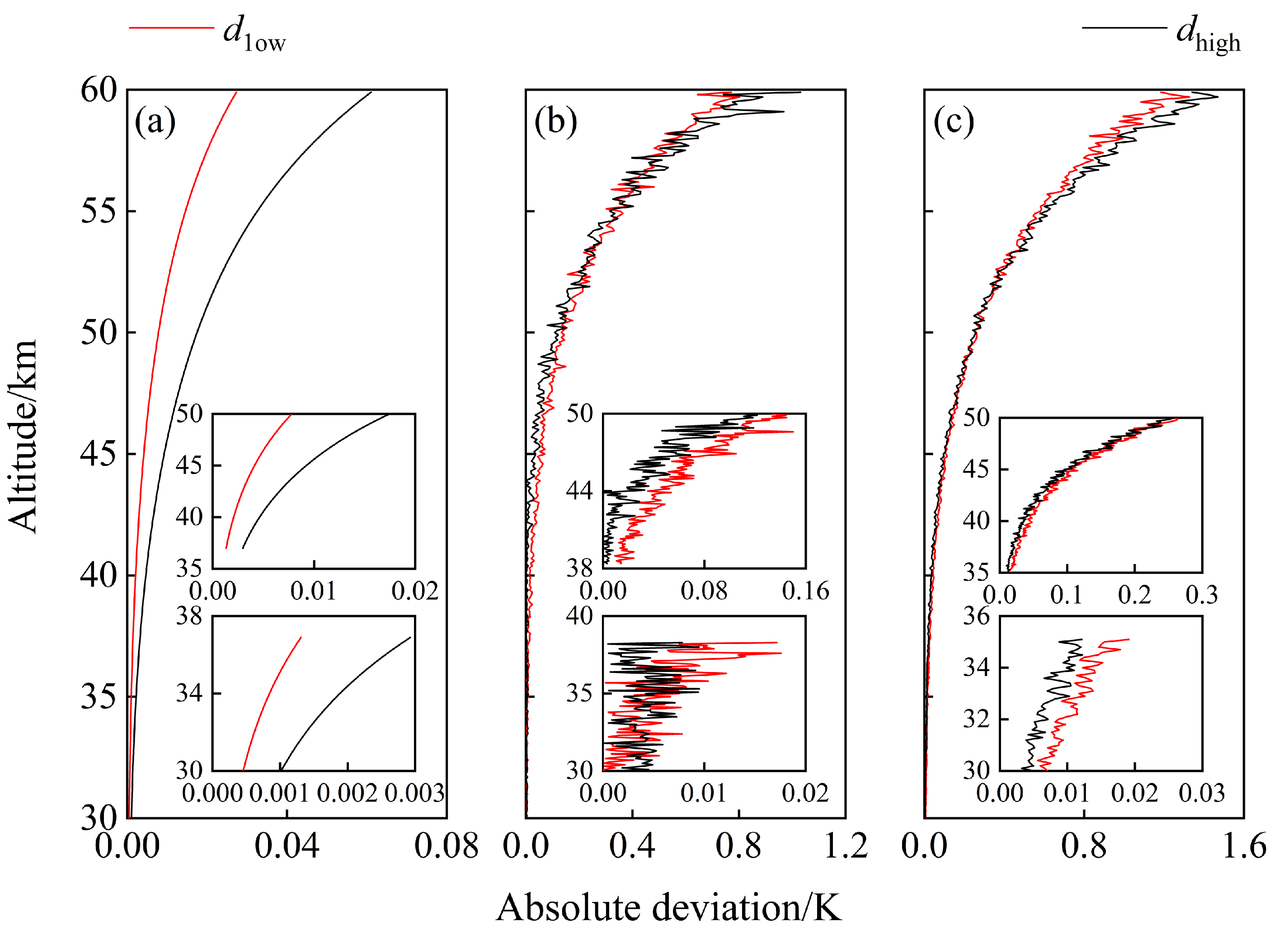
| Altitude Range (km) | Integration Time (s) | Component | Altitude Section (km) | Significant Digit | Numerical Tolerance |
|---|---|---|---|---|---|
| 30–50 | 60 | Auxiliary | 30–40 | 1 | 0.5 |
| Detection | 30–31.2 | 1 | 0.05 | ||
| 31.3–40 | 1 | 0.5 | |||
| Combined | 30–40 | 1 | 0.5 | ||
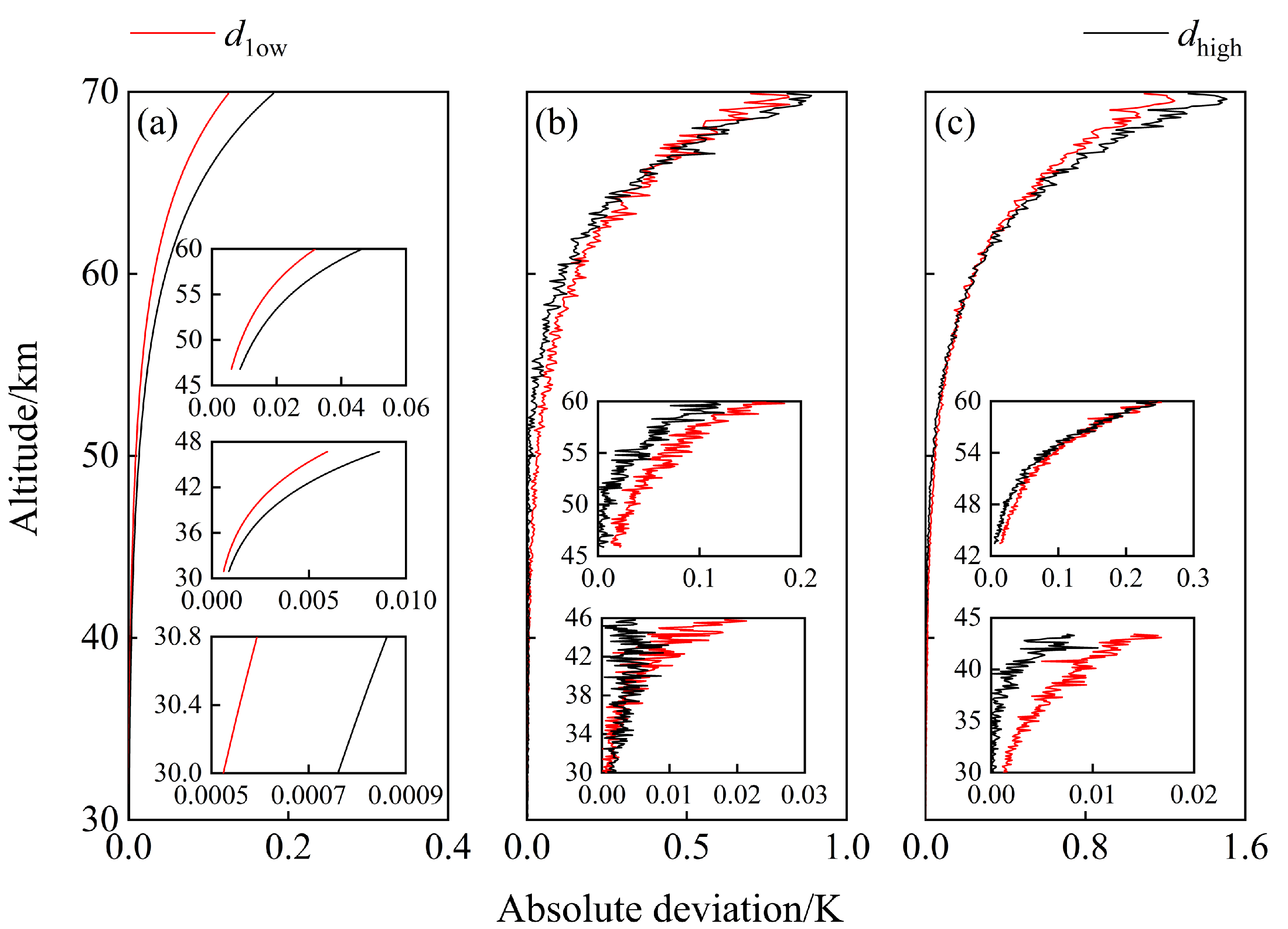
| 30–60 | 420 | Auxiliary | 30–36.9 | 1 | 0.05 |
| 37–50 | 1 | 0.5 | |||
| Detection | 30–38.3 | 1 | 0.05 | ||
| 38.4–50 | 1 | 0.5 | |||
| Combined | 30–35.1 | 1 | 0.05 | ||
| 35.2–50 | 1 | 0.5 | |||
| 30–70 | 2400 | Auxiliary | 30–30.8 | 2 | 0.005 |
| 30.9–46.7 | 1 | 0.05 | |||
| 46.8–60 | 1 | 0.5 | |||
| Detection | 30–45.8 | 1 | 0.05 | ||
| 45.9–60 | 1 | 0.5 | |||
| Combined | 30–43.4 | 1 | 0.05 | ||
| 43.5–60 | 1 | 0.5 |
Disclaimer/Publisher’s Note: The statements, opinions and data contained in all publications are solely those of the individual author(s) and contributor(s) and not of MDPI and/or the editor(s). MDPI and/or the editor(s) disclaim responsibility for any injury to people or property resulting from any ideas, methods, instructions or products referred to in the content. |
© 2023 by the authors. Licensee MDPI, Basel, Switzerland. This article is an open access article distributed under the terms and conditions of the Creative Commons Attribution (CC BY) license (https://creativecommons.org/licenses/by/4.0/).
Share and Cite
Li, X.; Zhong, K.; Zhang, X.; Wu, T.; Zhang, Y.; Wang, Y.; Li, S.; Yan, Z.; Xu, D.; Yao, J. Uncertainty Evaluation on Temperature Detection of Middle Atmosphere by Rayleigh Lidar. Remote Sens. 2023, 15, 3688. https://doi.org/10.3390/rs15143688
Li X, Zhong K, Zhang X, Wu T, Zhang Y, Wang Y, Li S, Yan Z, Xu D, Yao J. Uncertainty Evaluation on Temperature Detection of Middle Atmosphere by Rayleigh Lidar. Remote Sensing. 2023; 15(14):3688. https://doi.org/10.3390/rs15143688
Chicago/Turabian StyleLi, Xinqi, Kai Zhong, Xianzhong Zhang, Tong Wu, Yijian Zhang, Yu Wang, Shijie Li, Zhaoai Yan, Degang Xu, and Jianquan Yao. 2023. "Uncertainty Evaluation on Temperature Detection of Middle Atmosphere by Rayleigh Lidar" Remote Sensing 15, no. 14: 3688. https://doi.org/10.3390/rs15143688