Article

Enhancing Wheat Above-Ground Biomass Estimation Using UAV RGB Images and Machine Learning: Multi-Feature Combinations, Flight Height, and Algorithm Implications

1
Institute of Farmland Irrigation, Chinese Academy of Agricultural Sciences, Xinxiang 453002, China
2
School of Surveying and Land Information Engineering, Henan Polytechnic University, Jiaozuo 454003, China
3
Key Laboratory of Water-Saving Irrigation Engineering, Ministry of Agriculture & Rural Affairs, Xinxiang 453002, China
4
Key Laboratory of Water-Saving Agriculture of Henan Province, Xinxiang 453002, China
5
College of Land Science and Technology, China Agricultural University, Beijing 100193, China
*
Author to whom correspondence should be addressed.
Remote Sens. 2023, 15(14), 3653; https://doi.org/10.3390/rs15143653
Submission received: 5 June 2023 / Revised: 30 June 2023 / Accepted: 20 July 2023 / Published: 21 July 2023
(This article belongs to the Section Remote Sensing in Agriculture and Vegetation)

Abstract

:
Above-ground biomass (AGB) serves as an indicator of crop growth status, and acquiring timely AGB information is crucial for estimating crop yield and determining appropriate water and fertilizer inputs. Unmanned Aerial Vehicles (UAVs) equipped with RGB cameras offer an affordable and practical solution for efficiently obtaining crop AGB. However, traditional vegetation indices (VIs) alone are insufficient in capturing crop canopy structure, leading to poor estimation accuracy. Moreover, different flight heights and machine learning algorithms can impact estimation accuracy. Therefore, this study aims to enhance wheat AGB estimation accuracy by combining VIs, crop height, and texture features while investigating the influence of flight height and machine learning algorithms on estimation. During the heading and grain-filling stages of wheat, wheat AGB data and UAV RGB images were collected at flight heights of 30 m, 60 m, and 90 m. Machine learning algorithms, including Random Forest Regression (RFR), Gradient Boosting Regression Trees (GBRT), Ridge Regression (RR), Least Absolute Shrinkage and Selection Operator (Lasso) and Support Vector Regression (SVR), were utilized to construct wheat AGB estimation models. The research findings are as follows: (1) Estimation accuracy using VIs alone is relatively low, with R2 values ranging from 0.519 to 0.695. However, combining VIs with crop height and texture features improves estimation accuracy, with R2 values reaching 0.845 to 0.852. (2) Estimation accuracy gradually decreases with increasing flight height, resulting in R2 values of 0.519–0.852, 0.438–0.837, and 0.445–0.827 for flight heights of 30 m, 60 m, and 90 m, respectively. (3) The choice of machine learning algorithm significantly influences estimation accuracy, with RFR outperforming other machine learnings. In conclusion, UAV RGB images contain valuable crop canopy information, and effectively utilizing this information in conjunction with machine learning algorithms enables accurate wheat AGB estimation, providing a new approach for precision agriculture management using UAV remote sensing technology.

Graphical Abstract

1. Introduction

Crop above-ground biomass (AGB) refers to the organic matter fixed in crops during their growth process, which is closely influenced by factors such as photosynthesis, nutrient absorption, and climate [1]. Measuring crop AGB plays a crucial role in assessing crop growth status, determining fertilization requirements, promptly detecting pests and diseases, and predicting crop yield [2]. However, traditional manual sampling methods for measuring crop AGB are reliable but expensive, destructive, and limited in terms of the number of sampling points. Consequently, they are only suitable for small-scale agricultural areas and fail to meet the demand for quantitative monitoring of crop AGB over larger regions [3]. Hence, there is a need to explore more efficient, cost-effective, and dependable methods for acquiring timely crop AGB information.
Remote sensing technology enables the collection of crop canopy reflectance information from a distance, without direct contact. Analyzing and processing this reflectance information allows for non-destructive monitoring of crop growth [4]. In comparison to ground surveys, remote sensing technology offers real-time, non-destructive, and large-scale estimation of crop AGB [5]. Unmanned Aerial Vehicles (UAVs) remote sensing technology has proven effective in crop growth monitoring due to its affordability, ease of use, and high temporal and spatial resolution [6]. The primary sensors used in UAVs include RGB digital cameras, multispectral sensors, hyperspectral sensors, and LiDAR sensors [7,8]. Although multispectral, hyperspectral, and LiDAR sensors provide superior accuracy and versatility, their high cost and complexity limit their widespread application [9]. In contrast, RGB digital cameras are preferred for crop growth monitoring due to their cost-effectiveness, lightweight nature, high spatial resolution, and simplified data processing [10,11].
Numerous studies have demonstrated the effectiveness of estimating the AGB of wheat, maize, and rice by calculating vegetation indices (VIs) from UAV RGB images [12,13,14]. However, VIs alone are limited in capturing internal information of vertically growing crop organs, leading to lower accuracy in estimation [15]. To address this limitation, some studies have explored the combination of VIs with crop height (CH) [16]. CH provides insights into the vertical structure of crops and its variations reflect the health and nutritional status of crops, thereby aiding in AGB estimation [17]. UAV RGB images can be stitched together to generate a digital surface model (DSM), which, in turn, enables the derivation of crop height models for obtaining CH information [18]. Crop height models based on UAV remote sensing technology can provide accurate CH. When combined with VIs, they provide a novel approach for in-field estimation of crop AGB.
While VIs are commonly used indicators for estimating crop AGB, their accuracy can be influenced by various factors such as soil background, lighting conditions, and weather [19]. Moreover, VIs tend to lose sensitivity during the reproductive growth stage, limiting their effectiveness as standalone estimators of crop AGB. On the other hand, texture features are less susceptible to these factors and can provide valuable high-frequency information about crop growth status, including leaf morphology, distribution density, and leaf arrangement [20]. Texture features refer to the variations in grayscale distribution of pixels within their neighboring area, enabling them to reflect the spatial distribution of vegetation in the image and its relationship with the surrounding environment [21]. Therefore, combining VIs with texture features shows great potential in enhancing the accuracy of crop AGB estimation.
In UAV remote sensing, flight height is a crucial factor that influences image resolution and quality [22]. Currently, in studies aimed at estimating crop growth parameters, flight heights typically range from 30 to 100 m, corresponding to image resolutions of 1 to 10 cm [5,23]. However, the selection of flight heights and corresponding image resolutions in current research is subjective and arbitrary, lacking unified standards and guidelines. This lack of standardization poses challenges for the application and dissemination of crop growth parameter inversion models based on UAV remote sensing technology. Therefore, evaluating the impact of different flight height images on crop AGB estimation holds significant importance in formulating standardized guidelines for UAV image acquisition.
The continuous progress in artificial intelligence and computer science has propelled the development of machine learning algorithms, leading to their widespread application in agricultural remote sensing data analysis [24]. As a branch of machine learning, deep learning has experienced rapid growth. For instance, artificial neural networks (ANN) and convolutional neural networks (CNN) are two renowned deep learning algorithms that possess unique advantages and have been successfully applied in various fields. ANN excels in capturing complex nonlinear relationships within data and can generalize well to unseen samples with appropriate training [25]. It is effective in handling high-dimensional datasets, making it suitable for tasks such as image recognition and natural language processing. On the other hand, CNN is specifically designed for image processing tasks and is highly efficient in extracting spatial features from images [26]. It utilizes convolutional layers to automatically detect patterns and structures, exhibiting remarkable performance in object detection and image classification tasks. However, it is important to note that while ANN and CNN demonstrate promise in many applications, they also have limitations. Compared to traditional machine learning algorithms, deep learning algorithms typically require a large amount of labeled training data and longer training times. Additionally, the complex network architecture and hyperparameter tuning in deep learning models can pose challenges in terms of interpretability and computational resources [7]. Traditional machine learning algorithms, on the other hand, have certain advantages in interpretability, training speed, handling small-sample data, data requirements, and parameter optimization. Currently, traditional machine learning algorithms such as Random Forest Regression (RFR), Gradient Boosting Regression Trees (GBRT), and Support Vector Regression (SVR) are widely used for estimating various crop growth parameters, including monitoring corn leaf area index, estimating soybean yield, and assessing wheat nitrogen nutrition status [7,27,28]. It is worth noting that each machine learning algorithm operates based on its unique principles; therefore, when applied to the same dataset, they may yield different results. By understanding their distinct working principles, researchers can significantly improve the accuracy and reliability of crop growth parameter estimation. In addition to selecting suitable machine learning algorithms, feature importance analysis and hyperparameter tuning are of significant importance in the field of machine learning. Feature importance analysis helps us understand the essence of the data and enhance the model’s interpretability by determining the contribution of input features to the model’s prediction results [29]. On the other hand, reasonable selection of hyperparameters can enhance the accuracy and stability of the model, avoiding overfitting or underfitting and optimizing the utilization of computational resources [18]. Both of these processes are critical steps in optimizing the performance and interpretability of machine learning models, playing crucial roles in improving model performance and facilitating the practical application of machine learning.
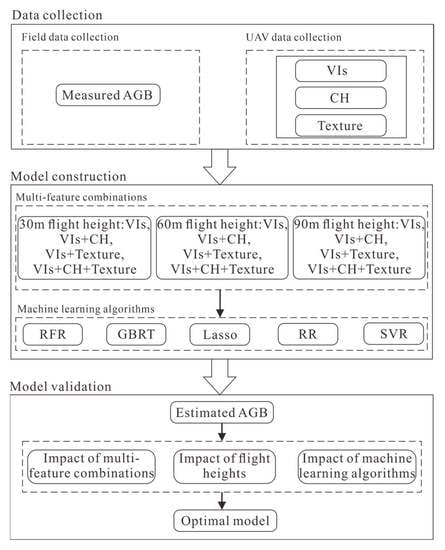
In summary, previous studies on wheat AGB estimation have solely relied on simple indicators such as VIs, making it difficult to accurately capture crop canopy structure and resulting in low estimation accuracy. Additionally, different flight altitudes and machine learning algorithms can also influence the estimation results. To address these issues, this study adopted the following approaches. Firstly, a comprehensive feature-based estimation method was proposed, integrating traditional VIs with CH and texture features to more accurately reflect wheat AGB. Secondly, the study explored the impact of different flight altitudes and multiple machine learning algorithms on estimation accuracy, thereby broadening the choice of UAV flight altitudes and methods for wheat AGB estimation. Therefore, the study puts forward the following hypotheses: (1) integrating VIs, CH, and texture features can more accurately reflect the growth status of wheat, hypothesizing that combining multiple features can improve estimation accuracy; (2) different flight altitudes may lead to variations in observing wheat canopy structure, hypothesizing that estimation accuracy decreases with increasing flight altitude; (3) different machine learning algorithms have different implementation principles, hypothesizing that the choice of different machine learning algorithms significantly affects wheat yield estimation accuracy. By validating these innovative methods and hypotheses, this study aims to provide new approaches and insights for accurately estimating wheat AGB and to offer new avenues for precision agricultural management based on unmanned aerial vehicle remote sensing technology.

2. Materials and Methods

2.1. Study Area and Experimental Design

The experiment was conducted at the Xinxiang Comprehensive Experimental Base of the Chinese Academy of Agricultural Sciences (Figure 1). Ten commonly cultivated wheat varieties were selected and planted on 25 October 2022. Six nitrogen fertilizer gradient treatments were applied (N1: 300 kg·hm−2, N2: 240 kg·hm−2, N3: 180 kg·hm−2, N4: 120 kg·hm−2, N5: 60 kg·hm−2, N6: 0 kg·hm−2), with each treatment consisting of 30 plots, resulting in a total of 180 plots. Each plot had dimensions of 4 × 1.2 m. Field irrigation management and pest control were carried out following the recommended local practices. To facilitate the subsequent processing of UAV images, 21 ground control points were established within the study area, and their accurate coordinates were obtained using Global Navigation Satellite System technology.

2.2. Field Data Acquisition

Wheat AGB data were collected at the heading and grain filling stages of wheat. The collection method was as follows: 10 uniformly growing wheat plants were randomly selected in each plot, sampled, and placed in sealed bags. The samples were then dried in a blast drying oven until the sample weight was stable and weighed. The AGB per unit area was calculated based on the planting density, and the AGB data for the heading (19 April) and grain filling (12 May) stages are shown in Table 1.

2.3. UAV Data Acquisition and Preprocessing

The UAV data acquisition part of this study used a DJI MAVIC 3M (SZ DJI Technology Co., Shenzhen, China) equipped with a high-definition digital camera including red, green, and blue colors with 5472 × 3468 pixels (Figure 2). The data collection was carried out on the same day as the wheat AGB collection. DJI Pilot 2 software version 6.1.1 (SZ DJI Technology Co., Shenzhen, China) was employed for flight route planning, with a flight height set at 30 m and both frontal and side overlap set at 80% to ensure data accuracy and reliability. To minimize variations in crop reflectance caused by uneven lighting conditions, the flights were conducted under clear and calm weather conditions, with consistent takeoff locations and flight routes for each flight. Furthermore, to investigate the impact of different flight heights on AGB estimation, UAV RGB image acquisition was also performed at 60 m and 90 m. Finally, the acquired RGB images were processed and stitched using Pix4D software version 4.4.12 (Pix4D, Lausanne, Switzerland). This involved tasks such as image import, ground control point tagging, image matching, point cloud generation, and the generation of digital orthophoto model and DSM.

2.4. Feature Extraction

2.4.1. Spectral Feature Extraction

The digital number (DN) values of the R, G, and B channels quantitatively reflect the radiation characteristics of the crop canopy in the visible spectrum. To minimize the impact of external environmental factors on crop reflectance, a normalization method was applied to normalize the DN values of the R, G, and B channels for each pixel. This normalization was conducted by dividing the DN values by the total DN values of the R, G, and B bands. In ArcMap software version 10.8 (Environmental Systems Research Institute, Inc., Redlands, CA, USA), a .shp file was created to delineate the boundaries of each plot, and the zonal statistics tool was utilized to extract the normalized DN values of the R, G, and B channels for each plot. These normalized DN values from the three channels were used to calculate VIs. Ten VIs closely associated with crop growth status were selected based on previous studies, as presented in Table 2 [10].
VIs are influenced by collinearity, and Principal Component Analysis (PCA) can extract the most representative principal components, reducing redundancy and mitigating the effects of multicollinearity among indices. PCA calculates the variance explained ratio of each feature, which indicates the contribution of each principal component to the total variance. Table 3 presents the variance explained ratio of the selected VIs in this study. From the results, it can be observed that EXG explains approximately 91.13% of the total variance, VARI explains approximately 8.38% of the total variance, and so on. In our results, the cumulative variance explained ratio of EXG, VARI, and EXGR has already exceeded 99.9%. This means that by retaining EXG, VARI, and EXGR, we can capture almost all of the variance information of the VIs, while the additional VIs provide relatively little information. Therefore, in this study, EXG, VARI, and EXGR were selected as inputs, as these VIs can effectively estimate wheat AGB.

2.4.2. CH Extraction

The RGB images of the bare soil period before wheat emergence, the heading stage, and the grain filling stage of wheat were used to create Digital Surface Models (DSMs) using Pix4D software. Next, the raster calculation tool in ArcMap software was employed to determine the difference between the DSMs at the heading and grain filling stages of wheat and the DSM at the bare soil period [18]. This calculation enabled the derivation of the corresponding CH at the heading stage, and the grain filling stage. Subsequently, the average CH for each plot was obtained using the mean method. This approach, based on DSMs, facilitated the acquisition of CH information, which formed a robust basis for subsequent wheat AGB estimation.

2.4.3. Texture Feature Extraction

In this study, the ENVI software version 5.3 (Harris Geospatial Solutions, Inc., Boulder, CO, USA) utilized used to compute gray-level co-occurrence matrix (GLCM), and the GLCM was utilized to extract texture features from the R, G, and B bands of the original images [27]. A total of seven texture features, including variance (Var), homogeneity (Hom), contrast (Con), dissimilarity (Dis), entropy (Ent), second moment (Sec), and correlation (Cor), were extracted [28]. Consequently, a total of 21 texture features were obtained from the R, G, and B channels for each growth stage. These extracted texture features provide valuable insights into the crop canopy information within the images and serve as a foundational component for subsequent wheat AGB estimation.

2.5. Machine Learning Algorithms

2.5.1. SVR

The objective of SVR is to construct a regression model that fits the data distribution by finding the solution to an optimization problem [18,28]. In SVR, data are mapped to a high-dimensional feature space, and an optimal hyperplane is found in that space to accommodate the target values to the maximum extent and minimize the gap between predicted and actual values. The parameters that need to be adjusted in SVR include the kernel function, which can be a linear, polynomial (poly), or radial basis function (rbf). The choice of an appropriate kernel function depends on the data’s characteristics and the nature of non-linear relationships. The C parameter is the regularization parameter that controls the model’s complexity and tolerance. Smaller C values result in a smoother model, while larger C values allow more training errors. In this study, the adjustment range for C is from 0.1 to 1, with a step size of 0.01. The gamma parameter is the width parameter for the rbf kernel. A smaller gamma value represents a broader basis function, while a larger gamma value makes the basis function narrower. In this study, the adjustment range for gamma is from 0.1 to 1, with a step size of 0.01. All machine learning algorithms in this study use grid search to try out different combinations of parameters and select the best performing ones.

2.5.2. Ridge Regression

Ridge Regression (RR) is a classical linear regression method used for handling regression data with collinearity [18]. It controls the complexity of the model by introducing an L2 regularization term, thereby reducing the risk of overfitting. The objective of Ridge Regression is to minimize the loss function, which is composed of the sum of squared residuals and the regularization term. The regularization term is the product of the sum of squared coefficients and a tuning parameter, alpha. When performing Ridge Regression, the parameter that needs to be adjusted is alpha. A smaller alpha value indicates weaker regularization, which may result in overfitting. On the other hand, a larger alpha value increases the strength of regularization, which may lead to underfitting. In this study, the range for adjusting alpha is from 0 to 0.03, with a step size of 0.001.

2.5.3. Least Absolute Shrinkage and Selection Operator

Least Absolute Shrinkage and Selection Operator (Lasso) is a linear regression method used for handling regression data with collinearity (i.e., high correlation among features) [33]. Compared to traditional linear regression methods, Lasso regression introduces an L1 regularization term that sets some feature coefficients to zero, effectively reducing the complexity of the model and the influence of features. When performing Lasso regression, the parameter that needs to be adjusted is alpha. In this study, the range for adjusting the alpha parameter in Lasso regression is from 0 to 0.03, with a step size of 0.001.

2.5.4. RFR

RFR is an ensemble learning algorithm that utilizes the predictions of multiple decision trees to make accurate estimations. It constructs each decision tree by randomly selecting a subset of features and samples from the dataset. The final prediction is obtained by averaging the predictions of these individual trees [5,34]. RFR offers several advantages, such as its ability to handle high-dimensional feature spaces, robustness, and reduction of overfitting risks [18]. Consequently, it is well-suited for various regression problems. The parameters that need to be adjusted in Random Forest Regression (RFR) include the number of decision trees (n_estimators) and the maximum depth of the trees (max_depth). The number of decision trees is crucial in RFR. Too few trees may result in underfitting, where the model lacks the ability to capture complex relationships in the data; on the other hand, having too many trees may lead to overfitting, where the model becomes overly complex and excessively fits the training data, resulting in poor generalization to new samples. In this study, the range for adjusting the number of decision trees is set from 50 to 1000, with a step size of 10. The maximum depth of the trees is another important parameter. A small tree depth limits the complexity of the model, potentially causing underfitting and the inadequate fitting of complex relationships in the data. Conversely, a large tree depth may lead to overfitting, where the decision trees become overly complex and overfit the training data, resulting in poor generalization. In this study, the range for adjusting the tree depth is set from 3 to 30, with a step size of 1.

2.5.5. GBRT

GBRT is a robust machine learning algorithm that combines decision trees with gradient boosting techniques, making it capable of handling nonlinear relationships, high-dimensional features, and complex datasets effectively. The fundamental concept behind GBRT is to train a sequence of decision tree models iteratively, where each model is trained based on the residuals of the previous model. During each iteration, GBRT optimizes the loss function using gradient descent, gradually minimizing the difference between predicted values and actual values to enhance the model’s accuracy [35]. The parameters that need to be adjusted for GBRT include the number of decision trees, the tree depth, and the learning rate. The adjustment range for the number of decision trees and tree depth is the same as for RFR. The learning rate is an important parameter for tuning the GBRT model. A smaller learning rate requires more decision trees to build the model, resulting in a better fit to the training data, but it may require longer training time. A larger learning rate can speed up the training process but may lead to overfitting, making the model overly sensitive to the training data and reducing its generalization ability. In this study, the learning rate for GBRT ranges from 0.01 to 0.1, with a step size of 0.01.

2.6. Accuracy Evaluation

In this study, a 5-fold cross-validation method was employed to evaluate the performance of machine learning algorithms, aiming to mitigate errors caused by random dataset splits [36]. The basic idea of this method is to randomly divide the dataset into 5 different subsets, with each subset taking turns as the test set while the remaining parts serve as the training set. This process is repeated 5 times to ensure that each subset is used as both training and test data. Finally, the average of the evaluation metrics obtained from the 5 test sets is used as an indicator to assess the model’s performance. The determination coefficient (R2) and relative root mean square error (rRMSE) were utilized as evaluation metrics in this study, and their calculation formulae are as follows [37]:
R 2 = 1 i = 1 n ( x i y i ) 2 i = 1 n ( x i y ¯ ) 2
rRMSE = i = 1 n ( x i y i ) 2 n y ¯ × 100 % ,
where xi is the measured AGB, yi is the estimated AGB, y ¯ is the mean of the measured AGB, and n is the number of samples in the test set.
Figure 3 illustrates the main workflow of this study, depicting the process from data acquisition to model construction and validation. First, various features are extracted from UAV RGB images at different heights (30 m, 60 m, and 90 m), including VIs, CH, and texture features. Concurrently, in-field wheat AGB data are collected as the target variable for the models. Subsequently, using these extracted features as inputs, machine learning algorithms such as RFR, GBRT, RR, Lasso, and SVR are employed to construct the wheat AGB estimation models. The primary focus of this study is to investigate the impact of feature combinations, UAV flight height, and the selection of machine learning algorithms on wheat AGB estimation. The findings aim to provide valuable technical support for precision agriculture management using UAVs.

3. Results

3.1. AGB Estimation by the Combination of VIs, CH, and Texture Features

The estimation of wheat AGB was performed using VIs and different feature combinations, as illustrated in Figure 4 and Table 4 (at a flight height of 30 m). Initially, the estimation was conducted solely using VIs, resulting in R2 values of 0.519–0.695 and rRMSE values of 17.00–21.31%. These values suggest that VI alone can only account for a portion of the variability in the estimation results. However, when VI was combined with CH, the estimated performance significantly improved. The R2 values increased to 0.830–0.850, and the rRMSE values decreased to 11.94–12.71%. These findings indicate that CH contributes to the estimation of wheat AGB, enhancing the model’s estimate capability. Furthermore, the incorporation of texture features alongside VI further enhanced the results. The R2 values improved to 0.772–0.835, and the rRMSE values decreased to 12.57–14.85%. This suggests that the inclusion of texture features positively influenced the estimation of wheat AGB, enhancing the accuracy of the model. Finally, the comprehensive fusion of VI, CH, and texture features demonstrated a significant improvement in estimating wheat AGB. The R2 values reached 0.845–0.852, and the rRMSE values were 11.84–12.17%. These results indicate that this multi-feature combinations approach can better capture the variability of wheat AGB and provide more accurate estimation results.
Figure 5 and Figure 6 present scatter plots depicting the estimation of AGB using VIs alone and the combination of VI with CH and texture features, respectively. Upon observing Figure 5 and Figure 6, it is evident that when AGB estimation is performed solely using VI, the scatter plot exhibits significant dispersion. This dispersion indicates a high level of uncertainty in the estimation results when relying solely on VIs. However, when VI is combined with CH and texture features (VIs + CH + Texture), a noticeable improvement is observed in the scatter plot. The scatter plot for VIs + CH + Texture demonstrates a trend closer to the 1:1 solid line, indicating a stronger alignment between the estimated AGB and the measured AGB. The results highlight that the combination of multi-features can improve the accuracy of AGB estimation for wheat and reduce bias in the estimation results.
After further research, this study analyzed the importance of each input feature using the built-in algorithm of RFR. The specific results are shown in Figure 7. The analysis results indicate that among the VIs, EXG has the highest importance score, reaching 14.47%. VARI comes next with an importance score of 2.28%, followed by EXGR with an importance score of 0.93%. This result is consistent with the results of PCA, where EXG explains 91.13% of the variance and also obtains the highest score in the feature importance analysis of VIs. For the texture features, regardless of the spectral band, the features Cor, Ent, Hom, and Sec all have relatively high importance scores, all over 1%. Among them, Cor has the highest importance score, exceeding 5% in all cases. Regarding the CH, the results show that it has an importance score of 12.12%, indicating its significant role in estimating AGB of wheat.

3.2. AGB Estimation at Different Flight Heights

In this study, AGB estimation for wheat was conducted using UAV RGB images captured at flight heights of 30 m, 60 m, and 90 m, as depicted in Figure 8 and Table 5. By way of the comprehensive Table 4 and Table 5, along with Figure 8, it becomes apparent that the estimation accuracy gradually decreases with increasing flight height. At a flight height of 30 m, the R2 values range from 0.519 to 0.852, and rRMSE ranges from 11.84% to 21.31%. These results indicate that the images captured at a flight height of 30 m provide relatively high accuracy and estimate ability, demonstrating excellent performance in AGB estimation for wheat. However, at a flight height of 60 m, the estimated R2 values range from 0.438 to 0.837, and rRMSE ranges from 12.41% to 23.35%. In comparison to the 30 m flight height, there is a slight decrease in estimation accuracy. Furthermore, at a flight height of 90 m, the estimated R2 values range from 0.445 to 0.827, and rRMSE ranges from 12.73% to 23.41%. It is evident that at higher flight heights, the AGB estimation results for wheat become less reliable, leading to a further decrease in estimation accuracy.

3.3. AGB Estimation Using Different Machine Learning Algorithms

Figure 9 illustrates the accuracy of various machine learning algorithms for estimating wheat AGB. The figure clearly demonstrates that RFR outperforms other machine learning processes of estimating wheat AGB. Furthermore, RFR exhibits a slightly better performance compared to GBRT.

4. Discussion

4.1. AGB Estimation Using VIs, CH, and Texture Feature Combination

VIs extracted from RGB images are simple and widely used spectral features for analyzing crop phenotypes. However, this study found that relying solely on VIs from RGB images may not accurately estimate wheat AGB. Similar findings were reported by Liu et al. [10], indicating the underestimation of crop AGB when using VIs from RGB images alone. This suggests that VIs from RGB images may not effectively capture the photosynthetic products stored in reproductive organs. The main reason for this limitation is that VIs from RGB images lacks the red-edge and near-infrared bands, which are sensitive to vegetation and have the potential to enhance vegetation vigor contrast [23,38]. Therefore, in this study, the estimation capability of VIs was found to be limited. However, it was observed that combining VIs with CH and texture features can significantly improve the estimation accuracy of wheat AGB. This finding is consistent with the results reported by Mao et al. [39], which also highlight the importance of combining multiple features to enhance crop AGB estimation accuracy. This is because different features can reflect crop information from different aspects, and the combination of multiple features can complement each other and effectively improve the accuracy of crop AGB estimation [25]. For example, VIs can quantitatively describe crop growth based on the reflectance of vegetation, but they are unable to capture detailed information about vegetation structure and composition [40]. In contrast, texture features can provide detailed information on vegetation characteristics, such as shape, size, and orientation, representing the high-frequency information of the crop [41]. Additionally, CH information can offer insights into the vertical structural information of vegetation, better reflecting the plant’s growth status [16]. Therefore, the combination of VIs, CH, and texture features allows for the utilization of different types of features, leading to improved estimation accuracy [18].
Additionally, this study analyzed the importance of each feature in estimating the AGB of wheat. Among the VIs, EXG obtained the highest importance score, reaching 14.47%. This could be attributed to EXG’s ability to effectively capture the differences between the green and red components in wheat images, providing crucial information about vegetation growth conditions [30]. Among the texture features, Cor exhibited higher importance scores compared to other features, all exceeding 5%. This may be because Cor is used to describe the degree of correlation between pixels in an image, representing pixel value similarity [21]. In wheat images, highly correlated pixels may indicate regions with similar colors and textures, which are related to the morphology and structure of wheat plants. For CH, it serves as an important indicator for assessing factors such as plant growth status and biomass accumulation [16]. Therefore, CH still maintains a substantial importance score of 12.12% in AGB estimation. In conclusion, all types of features have relatively high importance scores. This suggests that VIs, texture features, and crop height play important roles in estimating AGB in wheat.

4.2. Influence of Flight Height on Estimation Accuracy

In UAV remote sensing applications, flight height is a crucial parameter that affects several aspects, including spatial resolution, signal-to-noise ratio, and data acquisition cost [22]. The choice of flight height also has an impact on the estimation results for wheat AGB. This study suggests that a flight height of 30 m outperforms 60 m and 90 m, and this superiority can be attributed to several factors. Firstly, as shown in Figure 10, a flight height of 30 m provides a higher spatial resolution (0.81 cm/pixel) compared to 60 m (1.61 cm/pixel) and 90 m (2.42 cm/pixel). This higher resolution allows for more detailed information and greater accuracy in capturing the growth status and structural characteristics of wheat [4]. In contrast, higher flight heights result in decreased spatial resolution, making it challenging to detect subtle variations in AGB and reducing the accuracy of estimation. Secondly, the choice of flight height also affects the signal-to-noise ratio of the images. At lower flight heights, the camera captures clearer images, minimizing the impact of noise. Additionally, flying at a lower height reduces the distance between the ground and the sensor, mitigating the influence of atmospheric disturbances and enhancing the overall image quality [42]. This study focuses on the common flight altitudes of 30 m, 60 m, and 90 m to cover the range commonly used in practical UAV operations. Based on the results of this study, we have reason to believe that lower flight altitudes will result in higher estimation accuracy. However, it is important to consider the practical aspect of acquiring UAV remote sensing data, which involves cost considerations. Table 6 presents various costs required to complete the flight missions in this study. It is evident that a flight height of 30 m requires more flight time, waypoints, flight path length, and photo storage, thereby increasing the data acquisition cost. The selection of the optimal flight altitude should take into account data requirements, cost-effectiveness, feasibility, and mission objectives to ensure satisfactory results. For example, in crop breeding research, lower flight altitudes (e.g., 10–30 m) can provide higher image resolution and stronger capabilities in capturing crop details and spatial structures. This is crucial for breeders as they can analyze crop phenotypic features, genetic traits, and growth dynamics more accurately, thereby evaluating crop performance and selecting suitable varieties. In this case, higher estimation accuracy is necessary as even small differences can have a significant impact on crop breeding. However, for large-scale crop monitoring on farms, higher flight altitudes (e.g., 90 m or higher) may be more suitable. Although such altitudes may result in decreased image resolution, the impact of differences may be acceptable for crop monitoring across the entire farm. In this scenario, even with slightly reduced estimation accuracy, it is still possible to assess crop health, fertilization, irrigation needs, and take timely management measures. Therefore, within limited budgets and time frames, choosing higher flight altitudes may be more economical and feasible, while lower flight altitudes may be required for breeding research that demands higher accuracy.

4.3. Comparison of Different Machine Learning Algorithms

This study employed three different machine learning algorithms—RFR, GBRT, RR, Lasso and SVR—for estimating wheat AGB. The experimental results demonstrated that both RFR methods outperformed other machine learning methods in estimating wheat AGB, with RFR slightly outperforming GBRT in terms of overall performance. These findings indicate that RFR and GBRT methods effectively utilize information from UAV RGB images, thereby improving the accuracy of wheat AGB estimation. The superiority of RFR and GBRT methods can be attributed to their utilization of ensemble learning based on decision trees, which helps mitigate noise effects by aggregating multiple decision trees [43,44]. Notably, the slight advantage of RFR over GBRT may stem from the additional randomness introduced in the decision tree construction process, which reduces the risk of overfitting [45]. In comparison, SVR has the lowest estimation accuracy in this study, which may be because SVR is more sensitive to data volume and data quality. If there is insufficient data or outliers in the sample, the SVR model may not be able to accurately capture the pattern and trend of the data, resulting in a decrease in estimation accuracy [28]. In addition, the RR and Lasso methods exhibited lower performance in this experiment. This could be attributed to the complex nonlinear relationships between wheat AGB and various environmental factors and remote sensing indices [46,47]. RR and Lasso are based on linear relationships and perform poorly in regression analysis of nonlinear data [18,33]. In contrast, RFR and GBRT methods are capable of capturing relevant information from UAV RGB images through nonlinear modeling, enabling better estimation of wheat AGB. Furthermore, both RFR and GBRT methods possess advantages in estimating wheat AGB. For instance, they can handle large-scale datasets and exhibit robustness in handling outliers and noise, making them reliable and stable in practical applications [44,45,48].

4.4. Implications and Limitations of the Study

By utilizing a UAV equipped with an RGB camera, this study presents an economical and practical solution for efficiently obtaining wheat AGB information. The flexibility and adaptability of the UAVs allow data collection at different time points and locations, providing timely support for agricultural management decisions [5]. This study effectively improves the accuracy of wheat AGB estimation by combining VIs, CH, and texture features. Compared to methods that solely rely on VIs, the comprehensive analysis combining multiple features enhances the R2 value of the estimation results to 0.810–0.856, thereby more accurately reflecting the wheat AGB situation. Figure 11 illustrates the spatial distribution of wheat AGB estimated by the optimal model. Based on the spatial distribution map, it can be observed that wheat AGB shows an increasing trend with nitrogen application levels. This observation aligns with the mechanism of nitrogen promoting plant growth and nutrient uptake [26]. However, the impact of nitrogen application on biomass is still regulated by various factors. Therefore, in practical production, it is necessary to consider multiple factors comprehensively to improve the efficiency of farmland resource utilization and reduce costs and environmental impacts [22]. Furthermore, this study explores the influence of flight altitude and machine learning algorithms on estimation results. The results indicate that an increase in flight altitude gradually decreases the estimation accuracy, and different machine learning algorithms also have significant effects on estimation precision. This research not only provides estimation results but also offers valuable references for future research and applications.
However, this study only conducted data collection during the heading and grain filling stages of wheat, without covering other growth stages. This may lead to a partial understanding of wheat AGB variations. Future research should consider incorporating data from other growth stages to improve the model’s applicability and gain a more comprehensive understanding of changes in wheat AGB. Furthermore, this study was conducted only in Xinxing County, Henan Province. Different regions may have varying soil types and climate conditions, which play a crucial role in estimating AGB of crops. Firstly, different soil types possess distinct nutrient content, texture, and water retention capacity, directly influencing crop growth and AGB accumulation. Secondly, climate factors such as rainfall distribution, temperature variations, and sunshine hours are closely associated with crop growth and development. Therefore, when extrapolating this research method to actual farmland, it is essential to acknowledge the influence of these factors on estimation results and make corresponding adjustments and corrections. By collecting more extensive data and conducting field validation in diverse soil types and climate conditions, the applicability and accuracy of this research method can be further evaluated. This will provide more specific and accurate guidance for practical agricultural decision-making.

5. Conclusions

This study aimed to estimate wheat AGB using UAV RGB images and investigate the impact of various factors, including the combination of VIs with CH and texture features, flight height, and machine learning algorithms, on the accuracy of AGB estimation. The following conclusions can be drawn from the study:
  • Combining VIs with either CH or texture features improves the accuracy of AGB estimation compared to using VI alone. The highest accuracy was achieved when combining VI, CH, and texture features (VI + CH + texture) for wheat AGB estimation.
  • Flight height has a significant influence on the accuracy of AGB estimation. A flight height of 30 m resulted in higher accuracy. However, flight heights of 60 or 90 m can significantly reduce the acquisition costs of the flight mission. The choice of flight height should be based on specific mission requirements.
  • The selection of machine learning algorithms is crucial for wheat AGB estimation. In this study, the RFR algorithm outperformed other machine learning algorithms, leading to higher accuracy in AGB estimation.
In summary, the multi-feature combinations, appropriate flight height selection, and the use of effective machine learning algorithms can significantly enhance the accuracy of UAV remote sensing technology for estimating wheat AGB. These findings provide valuable insights and guidance for the application of UAV remote sensing technology in agricultural practices.

Author Contributions

Conceptualization, W.Z., Z.C. and C.L.; methodology, W.Z. and Z.C.; software, Q.C.; validation, W.Z., Y.L. and B.M.; formal analysis, W.Z.; investigation, S.F.; resources, F.D.; data curation, W.Z.; writing—original draft preparation, W.Z.; writing—review and editing, Q.C.; visualization, Z.L.; supervision, W.Z.; project administration, Z.C. and S.Q.; funding acquisition, Z.C. and S.Q. All authors have read and agreed to the published version of the manuscript.

Funding

This research was funded by Central Public-Interest Scientific Institution Basal Research Fund (No. IFI2023-29), the Intelligent Irrigation Water and Fertilizer Digital Decision System and Regulation Equipment (2022YFD1900404), the Key Grant Technology Project of Henan (221100110700), the National Innovation and Entrepreneurship Training Program for College Students (202210460019), and the Key Project of Science and Technology of the Henan Province (222102110038).

Data Availability Statement

Data available on request from the correspondence authors.

Acknowledgments

The authors would like to thank the anonymous reviewers for their kind suggestions and constructive comments.

Conflicts of Interest

The authors declare no conflict of interest.

References

  1. Geng, L.; Che, T.; Ma, M.; Tan, J.; Wang, H. Corn biomass estimation by integrating remote sensing and long-term observation data based on machine learning techniques. Remote Sens. 2021, 13, 2352. [Google Scholar] [CrossRef]
  2. Li, Z.; Zhao, Y.; Taylor, J.; Gaulton, R.; Jin, X.; Song, X.; Li, Z.; Meng, Y.; Chen, P.; Feng, H.; et al. Comparison and transferability of thermal, temporal and phenological-based in-season predictions of above-ground biomass in wheat crops from proximal crop reflectance data. Remote Sens. Environ. 2022, 273, 112967. [Google Scholar] [CrossRef]
  3. Kumar, A.; Tewari, S.; Singh, H.; Kumar, P.; Kumar, N.; Bisht, S.; Devi, S.; Nidhi; Kaushal, R. Biomass accumulation and carbon stock in different agroforestry systems prevalent in the Himalayan foothills, India. Curr. Sci. 2021, 120, 1083–1088. [Google Scholar] [CrossRef]
  4. Yue, J.; Yang, G.; Tian, Q.; Feng, H.; Xu, K.; Zhou, C. Estimate of winter-wheat above-ground biomass based on UAV ultrahigh-ground-resolution image textures and vegetation indices. ISPRS-J. Photogramm. Remote Sens. 2019, 150, 226–244. [Google Scholar] [CrossRef]
  5. Han, S.; Zhao, Y.; Cheng, J.; Zhao, F.; Yang, H.; Feng, H.; Li, Z.; Ma, X.; Zhao, C.; Yang, G. Monitoring Key Wheat Growth Variables by Integrating Phenology and UAV Multispectral Imagery Data into Random Forest Model. Remote Sens. 2022, 14, 3723. [Google Scholar] [CrossRef]
  6. Jin, X.; Zarco-Tejada, P.J.; Schmidhalter, U.; Reynolds, M.P.; Hawkesford, M.J.; Varshney, R.K.; Yang, T.; Nie, C.; Li, Z.; Ming, B.; et al. High-throughput estimation of crop traits: A review of ground and aerial phenotyping platforms. IEEE Geosci. Remote Sens. Mag. 2020, 9, 200–231. [Google Scholar] [CrossRef]
  7. Liu, S.; Jin, X.; Nie, C.; Wang, S.; Yu, X.; Cheng, M.; Shao, M.; Wang, Z.; Tuohuti, N.; Bai, Y.; et al. Estimating leaf area index using unmanned aerial vehicle data: Shallow vs. deep machine learning algorithms. Plant Physiol. 2021, 187, 1551–1576. [Google Scholar] [CrossRef]
  8. Zhang, Y.; Yang, Y.; Zhang, Q.; Duan, R.; Liu, J.; Qin, Y.; Wang, X. Toward Multi-Stage Phenotyping of Soybean with Multimodal UAV Sensor Data: A Comparison of Machine Learning Approaches for Leaf Area Index Estimation. Remote Sens. 2022, 15, 7. [Google Scholar] [CrossRef]
  9. Zhu, W.; Sun, Z.; Huang, Y.; Yang, T.; Li, J.; Zhu, K.; Zhang, J.; Yang, B.; Shao, C.; Peng, J.; et al. Optimization of multi-source UAV RS agro-monitoring schemes designed for field-scale crop phenotyping. Precis. Agric. 2021, 22, 1768–1802. [Google Scholar] [CrossRef]
  10. Liu, Y.; Feng, H.; Yue, J.; Li, Z.; Yang, G.; Song, X.; Yang, X.; Zhao, Y. Remote-sensing estimation of potato above-ground biomass based on spectral and spatial features extracted from high-definition digital camera images. Comput. Electron. Agric. 2022, 198, 107089. [Google Scholar] [CrossRef]
  11. Guo, Z.-C.; Wang, T.; Liu, S.-L.; Kang, W.-P.; Chen, X.; Feng, K.; Zhang, X.-Q.; Zhi, Y. Biomass and vegetation coverage survey in the Mu Us sandy land-based on unmanned aerial vehicle RGB images. Int. J. Appl. Earth Obs. Geoinf. 2021, 94, 102239. [Google Scholar] [CrossRef]
  12. Gée, C.; Denimal, E. RGB image-derived indicators for spatial assessment of the impact of broadleaf weeds on wheat biomass. Remote Sens. 2020, 12, 2982. [Google Scholar] [CrossRef]
  13. Guo, Y.; Fu, Y.H.; Chen, S.; Bryant, C.R.; Li, X.; Senthilnath, J.; Sun, H.; Wang, S.; Wu, Z.; de Beurs, K. Integrating spectral and textural information for identifying the tasseling date of summer maize using UAV based RGB images. Int. J. Appl. Earth Obs. Geoinf. 2021, 102, 102435. [Google Scholar] [CrossRef]
  14. Duan, B.; Fang, S.; Gong, Y.; Peng, Y.; Wu, X.; Zhu, R. Remote estimation of grain yield based on UAV data in different rice cultivars under contrasting climatic zone. Field Crop. Res. 2021, 267, 108148. [Google Scholar] [CrossRef]
  15. Fu, Y.; Yang, G.; Li, Z.; Song, X.; Li, Z.; Xu, X.; Wang, P.; Zhao, C. Winter wheat nitrogen status estimation using UAV-based RGB imagery and gaussian processes regression. Remote Sens. 2020, 12, 3778. [Google Scholar] [CrossRef]
  16. Yue, J.; Feng, H.; Jin, X.; Yuan, H.; Li, Z.; Zhou, C.; Yang, G.; Tian, Q. A comparison of crop parameters estimation using images from UAV-mounted snapshot hyperspectral sensor and high-definition digital camera. Remote Sens. 2018, 10, 1138. [Google Scholar] [CrossRef] [Green Version]
  17. Pipatsitee, P.; Eiumnoh, A.; Tisarum, R.; Taota, K.; Kongpugdee, S.; Sakulleerungroj, K.; Suriyan, C.-U. Above-ground vegetation indices and yield attributes of rice crop using unmanned aerial vehicle combined with ground truth measurements. Not. Bot. Horti Agrobot. Cluj-Napoca 2020, 48, 2385–2398. [Google Scholar] [CrossRef]
  18. Fei, S.; Hassan, M.A.; Xiao, Y.; Su, X.; Chen, Z.; Cheng, Q.; Duan, F.; Chen, R.; Ma, Y. UAV-based multi-sensor data fusion and machine learning algorithm for yield prediction in wheat. Precis. Agric. 2023, 24, 187–212. [Google Scholar] [CrossRef]
  19. Zhang, M.; Zhou, J.; Sudduth, K.A.; Kitchen, N.R. Estimation of maize yield and effects of variable-rate nitrogen application using UAV-based RGB imagery. Biosyst. Eng. 2020, 189, 24–35. [Google Scholar] [CrossRef]
  20. Luo, H.-X.; Dai, S.-P.; Li, M.-F.; Liu, E.-P.; Zheng, Q.; Hu, Y.-Y.; Yi, X.-P. Comparison of machine learning algorithms for mapping mango plantations based on Gaofen-1 imagery. J. Integr. Agric. 2020, 19, 2815–2828. [Google Scholar] [CrossRef]
  21. Haralick, R.M.; Shanmugam, K.; Dinstein, I.H. Textural features for image classification. IEEE Trans. Syst. Man Cybern. 1973, 610–621. [Google Scholar] [CrossRef] [Green Version]
  22. Qiao, L.; Gao, D.; Zhao, R.; Tang, W.; An, L.; Li, M.; Sun, H. Improving estimation of LAI dynamic by fusion of morphological and vegetation indices based on UAV imagery. Comput. Electron. Agric. 2022, 192, 106603. [Google Scholar] [CrossRef]
  23. Liang, Y.; Kou, W.; Lai, H.; Wang, J.; Wang, Q.; Xu, W.; Wang, H.; Lu, N. Improved estimation of aboveground biomass in rubber plantations by fusing spectral and textural information from UAV-based RGB imagery. Ecol. Indic. 2022, 142, 109286. [Google Scholar] [CrossRef]
  24. Zhang, X.; Zhang, K.; Sun, Y.; Zhao, Y.; Zhuang, H.; Ban, W.; Chen, Y.; Fu, E.; Chen, S.; Liu, J.; et al. Combining spectral and texture features of UAS-based multispectral images for maize leaf area index estimation. Remote Sens. 2022, 14, 331. [Google Scholar] [CrossRef]
  25. Kheir, A.M.; Ammar, K.A.; Amer, A.; Ali, M.G.; Ding, Z.; Elnashar, A. Machine learning-based cloud computing improved wheat yield simulation in arid regions. Comput. Electron. Agric. 2022, 203, 107457. [Google Scholar] [CrossRef]
  26. Yu, D.; Zha, Y.; Sun, Z.; Li, J.; Jin, X.; Zhu, W.; Bian, J.; Ma, L.; Zeng, Y.; Su, Z. Deep convolutional neural networks for estimating maize above-ground biomass using multi-source UAV images: A comparison with traditional machine learning algorithms. Precis. Agric. 2023, 24, 92–113. [Google Scholar] [CrossRef]
  27. Maimaitijiang, M.; Sagan, V.; Sidike, P.; Hartling, S.; Esposito, F.; Fritschi, F.B. Soybean yield prediction from UAV using multimodal data fusion and deep learning. Remote Sens. Environ. 2020, 237, 111599. [Google Scholar] [CrossRef]
  28. Ding, F.; Li, C.; Zhai, W.; Fei, S.; Cheng, Q.; Chen, Z. Estimation of Nitrogen Content in Winter Wheat Based on Multi-Source Data Fusion and Machine Learning. Agriculture 2022, 12, 1752. [Google Scholar] [CrossRef]
  29. Meng, S.; Zhong, Y.; Luo, C.; Hu, X.; Wang, X.; Huang, S. Optimal temporal window selection for winter wheat and rapeseed mapping with Sentinel-2 images: A case study of Zhongxiang in China. Remote Sens. 2020, 12, 226. [Google Scholar] [CrossRef] [Green Version]
  30. Woebbecke, D.M.; Meyer, G.E.; Von Bargen, K.; Mortensen, D.A. Color indices for weed identification under various soil, residue, and lighting conditions. Trans. ASAE 1995, 38, 259–269. [Google Scholar] [CrossRef]
  31. Meyer, G.E.; Neto, J.C. Verification of color vegetation indices for automated crop imaging applications. Comput. Electron. Agric. 2008, 63, 282–293. [Google Scholar] [CrossRef]
  32. Bendig, J.; Yu, K.; Aasen, H.; Bolten, A.; Bennertz, S.; Broscheit, J.; Gnyp, M.L.; Bareth, G. Combining UAV-based plant height from crop surface models, visible, and near infrared vegetation indices for biomass monitoring in barley. Int. J. Appl. Earth Obs. Geoinf. 2015, 39, 79–87. [Google Scholar] [CrossRef]
  33. Tibshirani, R. Regression shrinkage and selection via the lasso. J. R. Stat. Soc. Ser. B-Stat. Methodol. 1996, 58, 267–288. [Google Scholar] [CrossRef]
  34. Wang, X.; Wang, Y.; Zhou, C.; Yin, L.; Feng, X. Urban forest monitoring based on multiple features at the single tree scale by UAV. Urban For. Urban Green. 2021, 58, 126958. [Google Scholar] [CrossRef]
  35. Yang, L.; Zhang, X.; Liang, S.; Yao, Y.; Jia, K.; Jia, A. Estimating surface downward shortwave radiation over china based on the gradient boosting decision tree method. Remote Sens. 2018, 10, 185. [Google Scholar] [CrossRef] [Green Version]
  36. Cheng, M.; Jiao, X.; Liu, Y.; Shao, M.; Yu, X.; Bai, Y.; Wang, Z.; Wang, S.; Tuohuti, N.; Liu, S.; et al. Estimation of soil moisture content under high maize canopy coverage from UAV multimodal data and machine learning. Agric. Water Manag. 2022, 264, 107530. [Google Scholar] [CrossRef]
  37. Jin, X.; Li, Z.; Feng, H.; Ren, Z.; Li, S. Deep neural network algorithm for estimating maize biomass based on simulated Sentinel 2A vegetation indices and leaf area index. Crop J. 2020, 8, 87–97. [Google Scholar] [CrossRef]
  38. Li, W.; Niu, Z.; Chen, H.; Li, D.; Wu, M.; Zhao, W. Remote estimation of canopy height and aboveground biomass of maize using high-resolution stereo images from a low-cost unmanned aerial vehicle system. Ecol. Indic. 2016, 67, 637–648. [Google Scholar] [CrossRef]
  39. Mao, P.; Qin, L.; Hao, M.; Zhao, W.; Luo, J.; Qiu, X.; Xu, L.; Xiong, Y.; Ran, Y.; Yan, C.; et al. An improved approach to estimate above-ground volume and biomass of desert shrub communities based on UAV RGB images. Ecol. Indic. 2021, 125, 107494. [Google Scholar] [CrossRef]
  40. Li, M.; Wu, J.; Song, C.; He, Y.; Niu, B.; Fu, G.; Tarolli, P.; Tietjen, B.; Zhang, X. Temporal variability of precipitation and biomass of alpine grasslands on the northern Tibetan plateau. Remote Sens. 2019, 11, 360. [Google Scholar] [CrossRef] [Green Version]
  41. Zhang, C.; Huang, C.; Li, H.; Liu, Q.; Li, J.; Bridhikitti, A.; Liu, G. Effect of textural features in remote sensed data on rubber plantation extraction at different levels of spatial resolution. Forests 2020, 11, 399. [Google Scholar] [CrossRef] [Green Version]
  42. Li, M.; Yang, Q.; Yuan, Q.; Zhu, L. Estimation of high spatial resolution ground-level ozone concentrations based on Landsat 8 TIR bands with deep forest model. Chemosphere 2022, 301, 134817. [Google Scholar] [CrossRef] [PubMed]
  43. Feng, P.; Wang, B.; Liu, D.L.; Waters, C.; Xiao, D.; Shi, L.; Yu, Q. Dynamic wheat yield forecasts are improved by a hybrid approach using a biophysical model and machine learning technique. Agric. For. Meteorol. 2020, 285–286, 107922. [Google Scholar] [CrossRef]
  44. Wei, Z.; Meng, Y.; Zhang, W.; Peng, J.; Meng, L. Downscaling SMAP soil moisture estimation with gradient boosting decision tree regression over the Tibetan Plateau. Remote Sens. Environ. 2019, 225, 30–44. [Google Scholar] [CrossRef]
  45. Cheng, M.; Penuelas, J.; McCabe, M.F.; Atzberger, C.; Jiao, X.; Wu, W.; Jin, X. Combining multi-indicators with machine-learning algorithms for maize yield early prediction at the county-level in China. Agric. For. Meteorol. 2022, 323, 109057. [Google Scholar] [CrossRef]
  46. Fu, Y.; Yang, G.; Song, X.; Li, Z.; Xu, X.; Feng, H.; Zhao, C. Improved estimation of winter wheat aboveground biomass using multiscale textures extracted from UAV-based digital images and hyperspectral feature analysis. Remote Sens. 2021, 13, 581. [Google Scholar] [CrossRef]
  47. Tian, Y.; Huang, H.; Zhou, G.; Zhang, Q.; Tao, J.; Zhang, Y.; Lin, J. Aboveground mangrove biomass estimation in Beibu Gulf using machine learning and UAV remote sensing. Sci. Total Environ. 2021, 781, 146816. [Google Scholar] [CrossRef]
  48. Zha, H.; Miao, Y.; Wang, T.; Li, Y.; Zhang, J.; Sun, W.; Feng, Z.; Kusnierek, K. Improving unmanned aerial vehicle remote sensing-based rice nitrogen nutrition index prediction with machine learning. Remote Sens. 2020, 12, 215. [Google Scholar] [CrossRef] [Green Version]
Figure 1. Study area overview and experimental design: (a) boundaries of Henan Province, China; (b) boundaries of Xinxiang County; (c) RGB image of the study area.
Remotesensing 15 03653 g001
Figure 2. UAV system: (a) DJI MAVIC 3M; (b,c) wheat growth status at heading and grain filling stages.
Remotesensing 15 03653 g002
Figure 3. Workflow diagram.
Remotesensing 15 03653 g003
Figure 4. AGB estimation accuracy with different feature combinations: (a) R2; (b) rRMSE.
Remotesensing 15 03653 g004
Figure 5. Scatter plots of AGB estimation using Vis: (a) SVR; (b) RR; (c) Lasso; (d) GBRT; and (e) RFR.
Remotesensing 15 03653 g005
Figure 6. Scatter plots of AGB estimation using VIs + CH + Texture: (a) SVR; (b) RR; (c) Lasso; (d) GBRT; and (e) RFR.
Remotesensing 15 03653 g006
Figure 7. Feature importance of VIs, texture features, and CH.
Remotesensing 15 03653 g007
Figure 8. AGB estimation accuracy at different flight heights (30 m, 60 m, and 90 m): (a) R2; (b) rRMSE.
Remotesensing 15 03653 g008
Figure 9. AGB estimation accuracy using different machine learning algorithms: (a) R2; (b) rRMSE.
Remotesensing 15 03653 g009
Figure 10. RGB images at different flight heights (30 m, 60 m, and 90 m): (a) 30 m; (b) 60 m; (c) 90 m.
Remotesensing 15 03653 g010
Figure 11. Estimated spatial distribution of wheat AGB: (a) heading stages; (b) grain filling stages.
Remotesensing 15 03653 g011
Table 1. Wheat AGB statistics at heading and grain filling stages.
Growth StagesSample SizeMax (kg·hm−2)Min (kg·hm−2)Mean (kg·hm−2)SD (kg·hm−2)CV (%)
Heading1807012.02180.04958.71071.821.61
Grain filling18010,800.04480.08254.21280.315.51
SD: standard deviation; CV: coefficient of variation.
Table 2. Ten selected VIs in the study.
VIFormulationReference
Excess Green Index (EXG)2G − R − B[30]
Excess Blue Index (EXB)1.4B − G[15]
Green Leaf Index (GLI)(2G − R − B)/(2G + R + B)[15]
Visible Atmospherically Resistant Index (VARI)(G − R)/(G + R − B)[15]
Excess Green minus Red Index (EXGR)3G − 2.4R − B[31]
Red Green Blue Vegetation Index (RGBVI)(G2 − BR)/(G2 + BR)[31]
Modified Green Red Vegetation Index (MGRVI)(G2 − R2)/(G2 + R2)[32]
Normalized Green Red Difference Index (NGRDI)(G − R)/(G + R)[15]
Green Red Ratio Index (GRRI)R/G[15]
Normalized Difference Index (NDI)(R − G)/(R + G + 0.01)[31]
“R” represents the DN value of the red color band, “G” represents the DN value of the green color band, and “B” represents the DN value of the blue color band.
Table 3. Variance explained ratio of the ten VIs.
VIEXGVARIEXGRNGBDIEXRRGBVIMGRVIGLINGRDIEXB
variance explained ratio91.13%8.38%0.49%3.46 × 10⁻⁵%3.16 × 10⁻⁶%2.23 × 10⁻⁷%4.19 × 10⁻⁸%1.85 × 10⁻⁹%3.81 × 10⁻¹⁰%8.87 × 10⁻¹⁹%
Table 4. AGB estimation accuracy with different feature combinations.
Feature CombinationSVRRRLassoGBRTRFR
R2rRMSE (%)R2rRMSE (%)R2rRMSE (%)R2rRMSE (%)R2rRMSE (%)
VIs0.51921.310.52321.200.55220.580.66917.720.69517.00
VIs + CH0.84912.110.85011.940.85011.950.83012.710.84112.30
VIs + Texture0.77214.850.79713.950.83112.690.82512.980.83512.57
VIs + CH + Texture0.84912.040.85111.920.85011.940.84512.170.85211.84
Table 5. AGB estimation accuracy at different flight heights (60 m and 90 m).
Flight HeightsFeature CombinationSVRRRLassoGBRTRFR
R2rRMSE (%)R2rRMSE (%)R2rRMSE (%)R2rRMSE (%)R2rRMSE (%)
60 mVIs0.43823.350.44623.060.49521.990.64718.250.63718.56
VIs + CH0.82613.150.81312.920.81312.930.83012.700.83312.58
VIs + GLCM0.61419.320.69816.940.75015.480.83012.720.83712.43
VI + CH + GLCM0.82813.050.82712.420.83212.280.83812.420.83712.41
90 mVIs0.44523.410.50721.780.53721.180.62318.990.62918.84
VIs + CH0.51322.220.79713.780.79713.790.82113.090.82612.88
VIs + GLCM0.50822.030.68517.350.74915.460.76714.880.76514.98
VIs + CH + GLCM0.55421.130.80913.340.81413.180.81813.130.82712.73
Table 6. Acquisition cost required to complete the flight mission at different flight heights (30 m, 60 m, and 90 m).
Flight HeightsResolution (cm/pixel)Flight TimeWaypointsFlight Path Length (m)Photo Storage
30 m0.8112 m 53 s12783122
60 m1.616 m 39 s740431
90 m2.424 m 27 s427214
Disclaimer/Publisher’s Note: The statements, opinions and data contained in all publications are solely those of the individual author(s) and contributor(s) and not of MDPI and/or the editor(s). MDPI and/or the editor(s) disclaim responsibility for any injury to people or property resulting from any ideas, methods, instructions or products referred to in the content.

