
Application of a Randomized Algorithm for Extracting a Shallow Low-Rank Structure in Low-Frequency Reverberation

School of Marine Technology, Ocean University of China, Qingdao 266100, China
*
Author to whom correspondence should be addressed.
†
These authors contributed equally to this work.
Remote Sens. 2023, 15(14), 3648; https://doi.org/10.3390/rs15143648
Submission received: 19 June 2023
/
Revised: 20 July 2023
/
Accepted: 20 July 2023
/
Published: 21 July 2023
(This article belongs to the Special Issue Advanced Techniques for Water-Related Remote Sensing)
Abstract
:The detection performance of active sonar is often hindered by the presence of seabed reverberation in shallow water. Separating the reverberations from the target echo and noise in the received signal is a crucial challenge in the field of underwater acoustic signal processing. To address this issue, an improved Go-SOR decomposition method is proposed based on the subspace-orbit-randomized singular value decomposition (SOR-SVD). This method successfully extracts the low-rank structure with a certain striation pattern. The results demonstrate that the proposed algorithm outperforms both the original Go algorithm and the current state-of-the-art (SOTA) algorithm in terms of the definition index of the low-rank structure and computational efficiency. Based on the monostatic reverberation theory of the normal mode, it is established that the low-rank structure is consistent with the low-frequency reverberation interference striation. This study examines the interference characteristics of the low-rank structure in the experimental sea area and suggests that the interferences of the fifth and seventh modes mainly control the low-rank structure. The findings of this study can be applied to seafloor exploration, reverberation waveguide invariant (RWI) extraction, and data-driven reverberation suppression methods.
1. Introduction
The study of shallow-water active detection requires careful consideration of seabed reverberation, which poses significant challenges and is of utmost importance [1]. In shallow water, seafloor reverberation presents a significant obstacle to active sonar performance, as weak target echoes can easily be overwhelmed by reverberation interference. Reverberation clutter, which is caused by the inhomogeneity of the water column, discrete scatters on the seafloor, non-discrete seabed structures [2], and fish schools [3], exacerbates the undesired constant false alarm rate (CFAR) of active sonar.
To address these challenges, researchers have developed reverberation suppression and signal separation technologies. However, as seabed reverberation and transmitted signals are inseparable in the Fourier domain, processing methods in the wavelet domain [4] and fractional Fourier domain [5,6,7] have become increasingly significant. To enhance data quality, singular value decomposition (SVD) [8] and mode decomposition (MD) [9,10,11,12,13,14] techniques can be implemented at different stages of processing. Some studies suggest that the reverberation waveguide invariant (RWI) , calculated by reverberation interference striation (RIS) that represents the regular structure in the time–frequency domain, can be used to develop RWI-based methods for CFAR and estimating the reverberation level (RL) [15,16]. However, these methods focus on a single measurement, ignoring the internal relationship between multiple measurements and resulting in difficulties with data-driven requirements.
In the processing of reverberation data using optimization and matrix computation-based theories, the structural properties of multi-ping data matrices are of significant importance due to their inherent low-rank features. In [17], a unitary transformation is applied to the block Toeplitz matrix of received signals, and a fast approximate algorithm is devised for the approximation of the reverberation low-rank subspace. For the localization problem of receiver failure in reverberant environments, a matrix completion algorithm that relies on the low-rank characteristic is developed for the Hankel matrices of received signals [18]. The non-negative matrix factorization (NMF) algorithm is utilized to calculate the low-rank structure based on the non-negative multiplier criterion and has been demonstrated to be effective for underwater blind-separation cases of linear frequency modulation (LFM) signals [19,20]. Background separation algorithms, such as robust principal component analysis (RPCA) [21] and Go decomposition [22], have been introduced to separate reverberation, target echo, and noise in multi-ping received signals [23,24] when reverberation signals are viewed as interference backgrounds. Furthermore, a combination method of NMF and Go decomposition is presented to detect underwater targets [25].
However, the current multi-ping methods of reverberation separation [23,24,25] face three significant challenges. Firstly, the method’s application is restricted to high-frequency, short-range reverberation, while cases of low-frequency distant reverberation have not been validated. In contrast to high-frequency short-range reverberation, low-frequency distant reverberation, which can be regarded as a two-way long-range propagation process, is more susceptible to the environmental factors of water velocity disturbance [26], geoacoustics [27], waveguide effects [28,29], and environmental uncertainty [30], resulting in more intricate reverberation pings. Consequently, the low-rank structure of reverberation obtained from multi-ping reverberation will exhibit distinct characteristics due to the impact of frequency and propagation distance. Secondly, although the low-rank structure between different reverberation pings is naturally introduced, a strictly physical explanation in specific scenarios has not been observed, resulting in the inability to guarantee the accuracy and effectiveness of the algorithm’s applicability and separation results. Thirdly, the existing methods mainly achieve signal separation through simulation and only a few have been validated at the level of experimental data, which may lead to uncertainties in the practical application of the algorithms.
To tackle the aforementioned issues, an efficient Go-SOR decomposition algorithm is proposed for separating reverberation signals. The algorithm is demonstrated to be effective for low-frequency and distant cases in underwater reverberant environments. Additionally, the results indicate that the proposed algorithm outperforms both the original Go algorithm and the state-of-the-art (SOTA) algorithm in terms of the definition index of the low-rank structure and computational efficiency. Furthermore, the physical significance of the low-rank structure obtained by the algorithm for low-frequency reverberation in shallow water is explicated as follows: under the monostatic reverberation model of the normal mode, the low-rank structure reverberation aligns with the theoretically predicted RIS. The experimental findings in the South China Sea reveal that the low-rank structure reverberation is primarily formed by the interference of the fifth and seventh modes, thereby ensuring the existence of a low-rank structure in shallow seabed reverberation.
1.1. Notations
- c, : minimum sound velocity in the water column, the sound velocity of seabed sediment.
- , , : width of the elliptical ring, area increment of bottom scattering, increment of polar angle.
- e: base of the natural logarithm.
- : distribution of RWI.
- : expectation of .
- f, : frequency point, interference frequency of mode m and .
- , : scattering amplitude of mode m and n at polar angle , scattering amplitude of mode m and n.
- i: square root of .
- , , : reverberation intensity, reverberation intensity matrix, mean value of reverberation intensity matrix.
- , , , : q-th ping of reverberation intensity, low-rank structure, sparse signal, and residual signal.
- j: iteration index in the algorithms.
- , , , : horizontal wavenumbers (eigenvalues) of different modes.
- : focal length of an ellipse.
- : low-rank matrix without the ping number (each ping is the same).
- m, , n, : mode numbers.
- , : maximum value of , minimum value of .
- N: total number of modes.
- p: oversampling the dimension parameter.
- , : reverberation pressure at polar angle , total reverberation pressure.
- , : retain the first k-largest absolute entries of a matrix and set other entries to zero (k-largest non-negative projection on matrix domain), hard threshold operator with threshold on the entries of a matrix .
- q, : index of the power scheme in the paper, index of reverberation pings.
- Q: total number of reverberation pings.
- ,: unitary\orthogonal matrix of QR decomposition.
- r, , , : rank of a matrix, the horizontal distance of monostatic reverberation, the horizontal distance from scatters to the receiver of bistatic reverberation, the horizontal distance from the source to the scatters of bistatic reverberation.
- : real field.
- , : upper triangular matrix of QR decomposition.
- : element of random amplitude in the scattering matrix.
- , : rank of a matrix , number of non-zero elements in a matrix .
- : soft threshold operator for with threshold .
- t, : reverberation time, maximum iterations.
- : element of the random scattering matrix without area term.
- , , , , , : unitary\orthogonal matrix of SVD.
- , : vectorization of a matrix , matricization of a vector .
- , , , : input matrix, low-rank matrix, sparse matrix, residual matrix.
- , , : depth of the source, depth of the receiver, depth of the bottom.
- : random variable with uniform distribution in at reverberation time t.
- , , : constants of Lambert amplitude.
- : sound absorption coefficient.
- : value of RWI.
- , : circular similarity of the ellipse at polar angle , bottom density.
- , , : polar angle, grazing angle of mode m, grazing angle of mode n.
- : hard threshold parameter.
- , , : diagonal matrix of SVD.
- : width of the transmitted pulse.
- : error margin.
- , , , : eigenfunctions of different depths and mode numbers.
- : Frobenius norm of a matrix .
- , , , : complex conjugation of , transpose\Hermitian transpose of a real\complex matrix , inverse of , Moore–Penrose inverse of a matrix .
- : ensemble operation.
2. Theoretical Basis of Seabed Distant Reverberation
2.1. Reverberation Model
A depth-projection schematic of the bistatic bottom reverberation model in shallow water is shown in Figure 1a. The black solid and cyan circles represent the source and receiver, respectively. The geometric prior yields an elliptical ring of width for the received reverberation at time t, with a fixed focal length . An area element on the elliptical ring is shown as a red square, and the solid blue line with an arrow indicates the projected path from the source to the receiver. Then, it is shown
Based on the normal mode reverberation theory [31,32], the seabed reverberation field corresponding to the unit scattering area can be expressed as
For simplicity, we omit the index of the polar angle in the scattering amplitude :
where the bottom scattering amplitude can be a empirical constant in the Lambert scattering case [33], or follows a Rayleigh or K distribution in the stochastic scattering case [34]; is a random variable with uniform distribution in and is the grazing angle of the m-th mode. More information can be found in the Notations section (Section 1.1). Integrating along angle in Equation (2), the reverberation field can be expressed as follows:
According to the geometric properties of an ellipse, and can be written as follows:
The bistatic seabed reverberation in shallow water can be deduced from Equations (4) and (5). We define the circular similarity as
When the ratio of the focal length to the length of the scattering path approaches zero, , and Equation (5) can be approximated as
which means that the scattering elliptic ring of bistatic reverberation can be regarded as the scattering circle ring of the monostatic case. Substituting Equation (7) into (4) yields the monostatic reverberation field
The corresponding schematic of monostatic reverberation is shown in Figure 1b, and the legends remain the same as in Figure 1a.
Figure 1.
Schematic of the shallow seabed reverberation. (a) Projection of the in-depth direction of the bistatic reverberation: elliptic ring. (b) Monostatic reverberation: circle ring.
Figure 1.
Schematic of the shallow seabed reverberation. (a) Projection of the in-depth direction of the bistatic reverberation: elliptic ring. (b) Monostatic reverberation: circle ring.

2.2. Simulations of Low-Frequency Bottom Reverberation
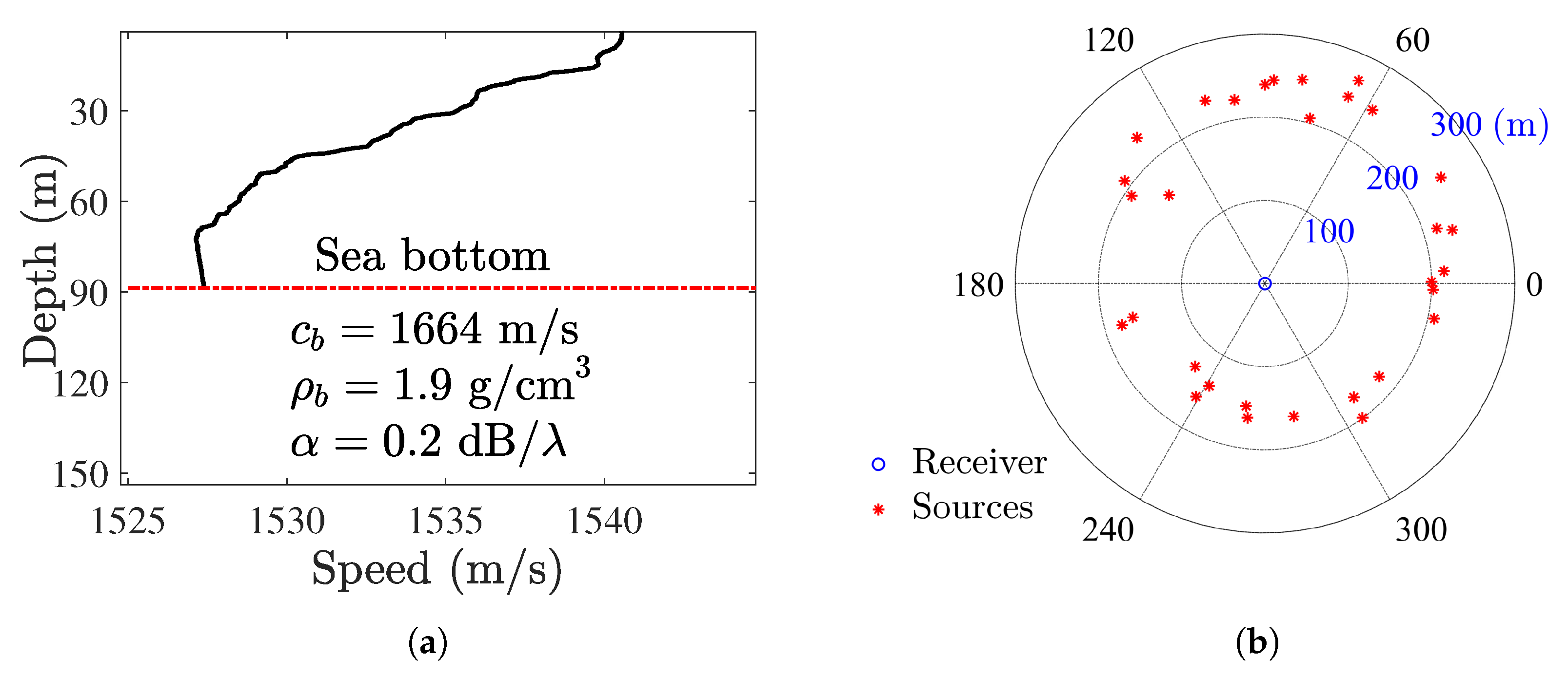
A sound speed profile (SSP) of the South China Sea is shown in Figure 2a. The SSP represents a negative gradient structure with a water depth of m. The bottom velocity , density , and absorption coefficients are 1664 m/s, 1.9 g/cm, and 0.2 dB/, respectively. The depths of the source and of the receiver are 50 m and 65 m, and the reverberation time and frequency bands are 2–6 s and 300–555 Hz, respectively. For the bistatic reverberation case, the focal length is set to 200 m.
Considering the reverberation field , the reverberation intensity can be expressed as follows:
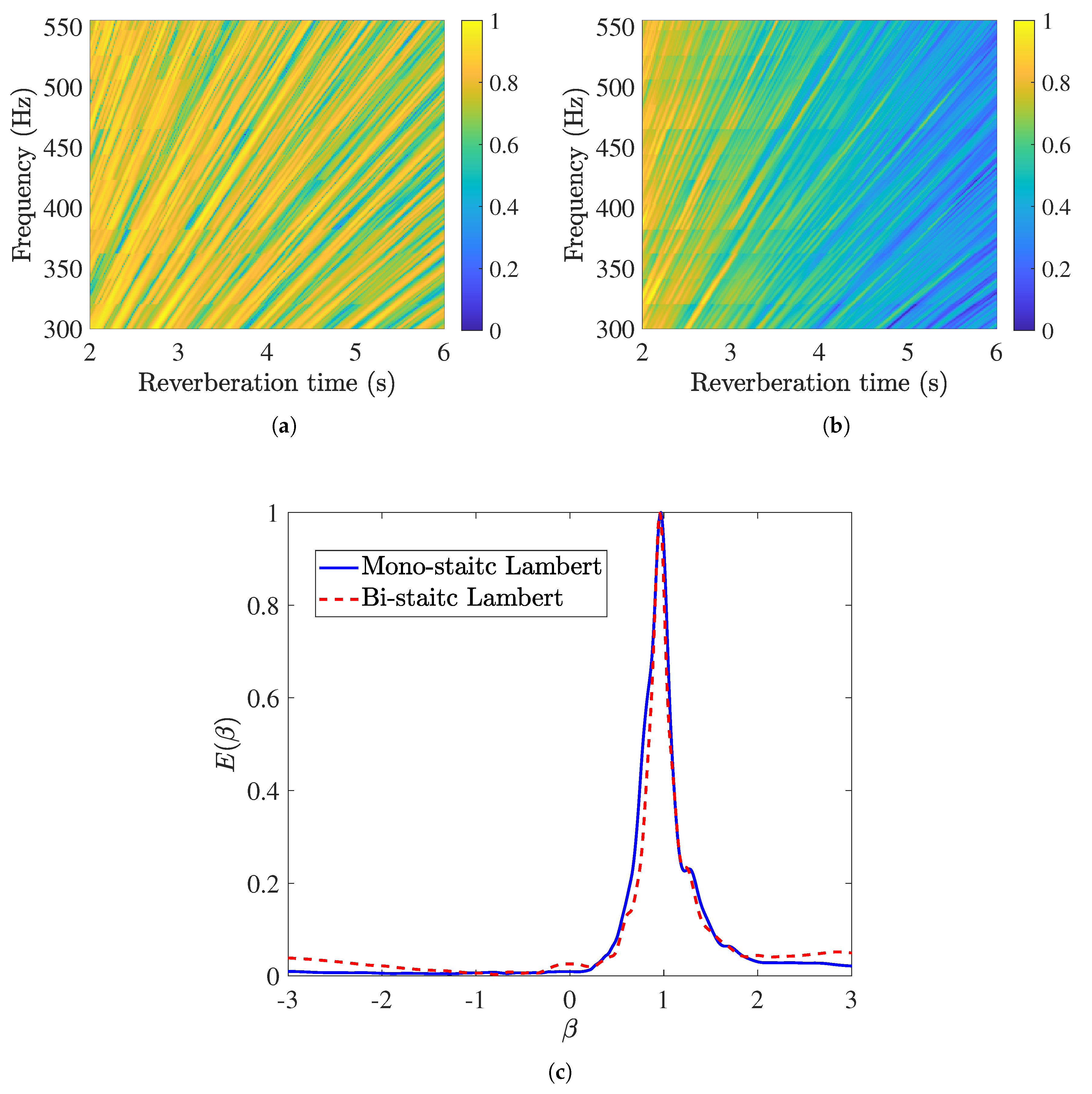
Simulated by Equations (8) and (9), the Lambert RIS for the monostatic case is shown in Figure 3a. By Equations (4) and (9), the Lambert RIS for the bistatic case is shown in Figure 3b. It can be seen that the slope information of the bistatic RIS is nearly the same as that of the monostatic RIS, but the intensity information differs. To measure the RISs, a two-dimensional Fourier transform method [35] (see Appendix A) is applied to calculate the distribution of RWI. The results are presented in Figure 3c, where the blue solid line and the red dashed line represent of the monostatic Lambert RIS in Figure 3a and bistatic Lambert RIS in Figure 3b, respectively, and are in good agreement with the peaks and trends. The peak distribution is conventionally defined as the real value of RWI, i.e., . Furthermore, when the simulating condition satisfies the reverberation time s, the circular similarity in Equation (8) satisfies . Thus, the bistatic bottom reverberation can be well-depicted by a much simpler monostatic bottom reverberation model in both theoretical and simulated bases under the given conditions.
3. Randomized Algorithms and Signal Separation
3.1. Randomized Form of Low-Rank Approximation
The Eckart–Young theorem [36] states that the optimal solution for low-rank approximation can be achieved through SVD under the constraint of the minimum Frobenius norm or spectral norm. However, the efficiency of SVD is limited by the size of the data matrix, and it is computationally expensive for large-dimensional matrices. To overcome this limitation, randomized algorithms based on the Johnson–Lindenstrauss theorem [37] have been introduced into SVD or low-rank approximation methods. Randomized SVD (RSVD) was first proposed by Halko et al. [38], then some researchers developed the subspace-orbit RSVD (SOR-SVD) [39,40] and theoretically provided the approximate error. Additionally, the low-rank approximation derived directly by the bilateral random projection (BRP) approach was first described in Equation (8) in [41], and optimized to the tight rank-r form by Zhou et al. [42], with a theoretical analysis of the approximate error under the constraint of the spectral norm.
The pseudocode implementations of the two randomized low-rank approximation methods, BRP and SOR-SVD, are presented in Algorithms 1 and 2, respectively. BRP and SOR-SVD are demonstrated to be strictly equivalent when and approximately equivalent when (refer to Appendix B). However, the efficiency of SOR-SVD is proved much better than that of BRP in the following content, especially when the power scheme parameter q increases.
| Algorithm 1 BRP with the power scheme |
| Input: , standard Gaussian matrix , r, q Output: low-rank matrix of rank r
|
| Algorithm 2 SOR-SVD with power scheme |
| Input: , standard Gaussian matrix , p, r, q Output: low-rank matrix of rank p, rank-r approximate SVD of
|
3.2. Algorithms of Signal Separation
As shown in Algorithm 3, the original Go decomposition is a signal separation algorithm based on alternating projection and the BRP–low-rank approximation [22]. For the following optimization problem:
the solution of the Go decomposition yields the low-rank background , sparse target signal , and residual noise corresponding to the input matrix .
As discussed in Section 3.1, the efficiency of BRP in the Go decomposition is lower than to that of SOR-SVD. Therefore, replacing BRP with SOR-SVD can reduce the computing time without sacrificing approximate precision. An improved algorithm, named Go-SOR, is presented in Algorithm 4. The SOTA randomized-separation algorithm, ALM-SOR-SVD RPCA [40], is also introduced in Algorithm 5 for comparison.
| Algorithm 3 Original Go decomposition |
| Input: , standard Gaussian matrix , r, q, k, , Output: low-rank matrix , sparse matrix , residual matrix
|
| Algorithm 4 Go-SOR decomposition |
| Input: , standard Gaussian matrix , r, q, k, , Output: low-rank matrix , sparse matrix , residual matrix
|
| Algorithm 5 ALM-SOR-SVD RPCA |
| Input: , standard Gaussian matrix , p, r, q, , Output: low-rank matrix , sparse-plus-noise matrix
|
Note that the output matrix of the ALM-SOR-SVD RPCA differs from that of the Go-SOR decomposition. Alternatively, the sparse matrix and residual matrix can be separated from the sparse-plus-noise matrix by applying a k-largest non-negative projection as follows:
where the subscript “” and the operation “max” with a parameter “l” indicates the index of elements and the l-th maximum in the matrix, respectively. Similarly, the element-wise hard threshold operator with a threshold on is applied in Go-SOR and is defined as follows:
4. Results
4.1. Low-Rank Structure of the Shallow Reverberation Experiment
Experimental data of shallow seabed reverberation were obtained from the 2015 reverberation experiment in the South China Sea. The SSP of the sea area is shown in Figure 2a, and the geoacoustic parameters are the same as those used in the simulation. The receiver was fixed at a depth of 65 m, and 31 explosive sources were released at a depth of 50 m around the receiver. The relative positions of the sources and the receiver are shown in Figure 2b, where the symbols of the blue circle and red asterisks indicate the receiver and sources, respectively. The distances between the sources and receiver are approximately 200 m. According to the results in Section 2, it is reasonable to simplify the experimental bistatic reverberation by monostatic reverberation when the reverberation time is s and the focal length is m.
The moving signal was not predetermined during the sea trial. Low-frequency analysis and recording (LOFAR) spectra of the experimental reverberation data were obtained by short-time Fourier transform (STFT) and labeled LOFARgram. LOFARgrams , , , and of ping numbers 1, 11, 21, and 31 are displayed in Figure 4a, Figure 4b, Figure 4c, and Figure 4d, respectively. It can be observed that these spectrograms vary with different pings, and there is no obvious regularity for the environmental uncertainty and difference in positions. The structural similarity index measure (SSIM) values of every two pings are shown in Table 1, and the results are concentrated around 0.1, which indicates the non-correlation of different reverberation pings.
The input matrix is obtained by the vectorization of different LOFARgrams
The initialization of Go-SOR (found in Algorithm 4), Go (found in Algorithm 3), and ALM-SOR-SVD RPCA (found in Algorithm 5) are , , and . Because there is no preset target for the experiment, the values of k and are meaningless. The low-rank matrix , sparse matrix , and residual matrix of q-th ping LOFARgram are obtained by the matricization of the output
The computing times of the three algorithms are listed in Table 2. These algorithms ran on a personal desktop computer equipped with an Intel i7 10700 CPU and 64 GB RAM, using Matlab 2022b software for implementations. It can be seen that the proposed Go-SOR algorithm (computing time 0.44 s) has a certain improvement compared to the SOTA performance of ALM-SOR-SVD RPCA (computing time 0.76 s). However, the original Go algorithm has the poorest performance (computing time 55.20 s) and takes two orders of magnitude longer than the other two algorithms. The improvement in efficiency of the proposed Go-SOR algorithm can be attributed to two factors: (a) the use of SOR-SVD instead of BRP in the low-rank approximation, and (b) the use of the hard threshold operator instead of the non-negative projection operator in each iteration [43]. The first factor was explained in detail earlier, and the second factor will be briefly discussed below. The non-negative projection operator involves time-consuming element-sorting, while the hard threshold operator is a more efficient operator that involves element subtraction. Additionally, the parameters of ALM-SOR-SVD RPCA are difficult to determine, whereas those of Go-SOR are relatively simple, which is a significant advantage in practical applications.
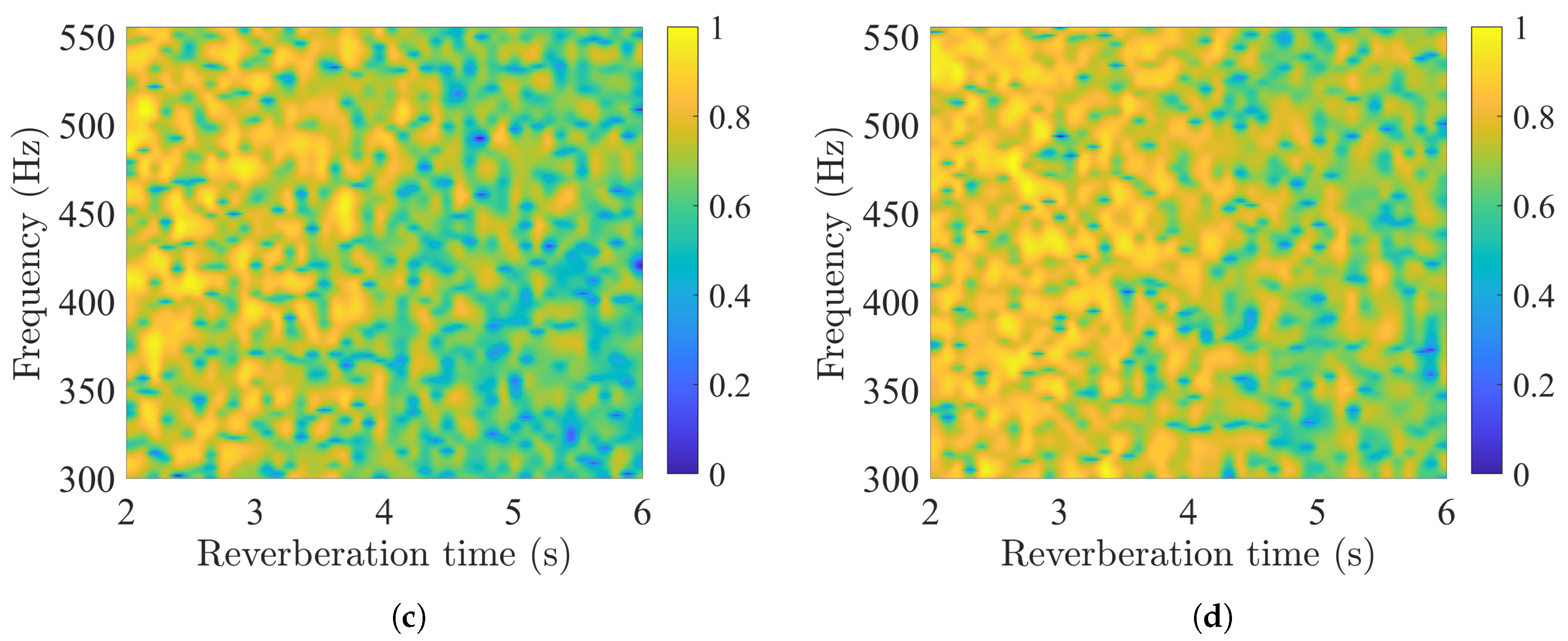
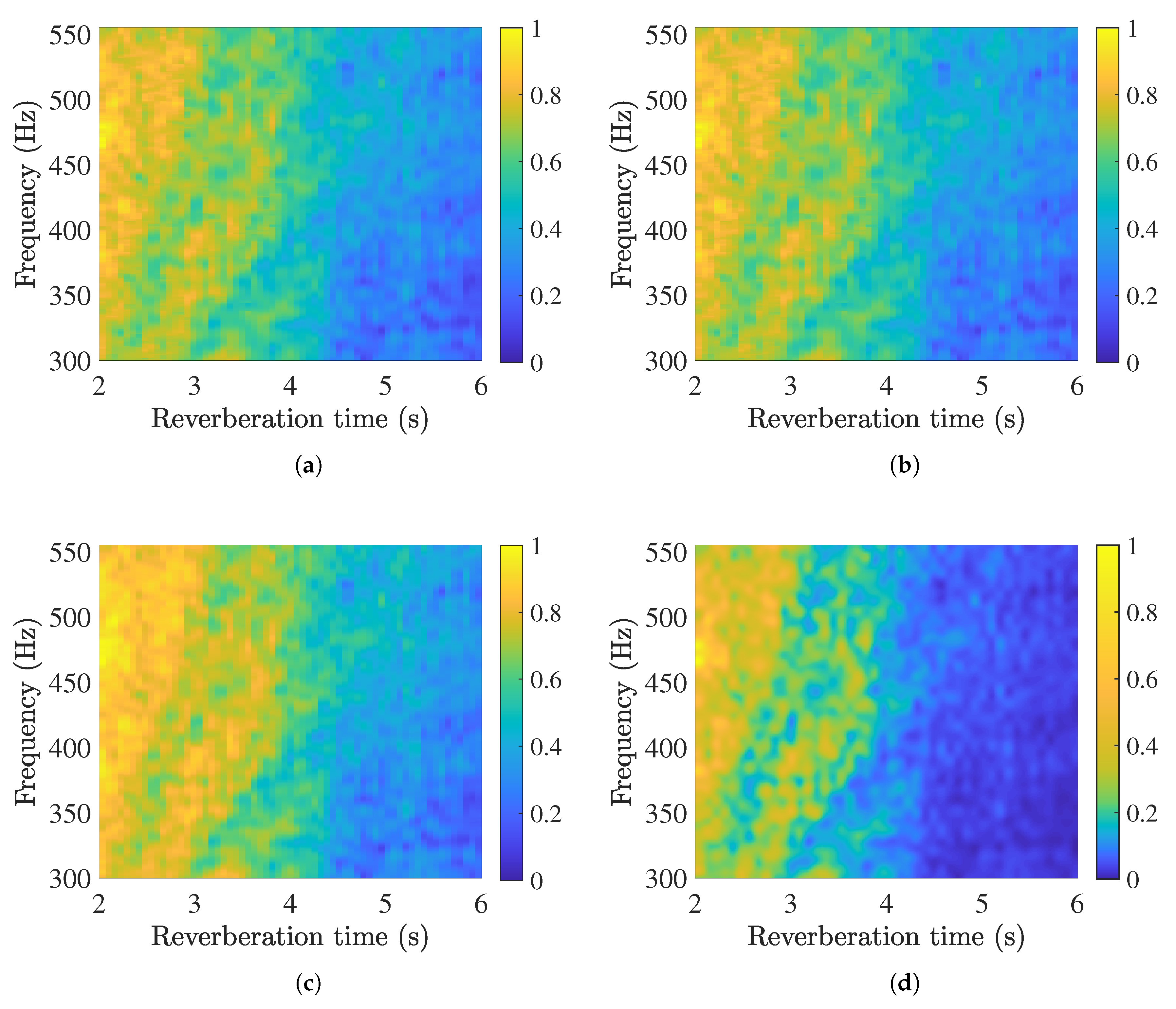
The low-rank structures for the three algorithms are shown in Figure 5. Figure 5a–c represent the results of Go-SOR, original Go, and ALM-SOR-SVD RPCA, respectively. The graph in Figure 5d symbolizes the mean LOFARgram of 31 reverberation pings. Although all four graphs show similar interference striation patterns around 2 s to 4.5 s, the low-rank structure of Go-SOR is the most distinct. The definition index, which is commonly used in optical image quality assessment, is calculated using four different matrix gradient methods: Energy of gradient (EOG), Tenengrad, Brenner, and Laplacian [44,45]. The results in Table 3 demonstrate that the proposed Go-SOR algorithm outperforms the other two algorithms in all four gradient methods, with the definition indices normalized to 1 for ease of understanding and comparison. Therefore, the proposed Go-SOR algorithm achieves the best performance in terms of both the image quality of the generated low-rank structure and computing efficiency.
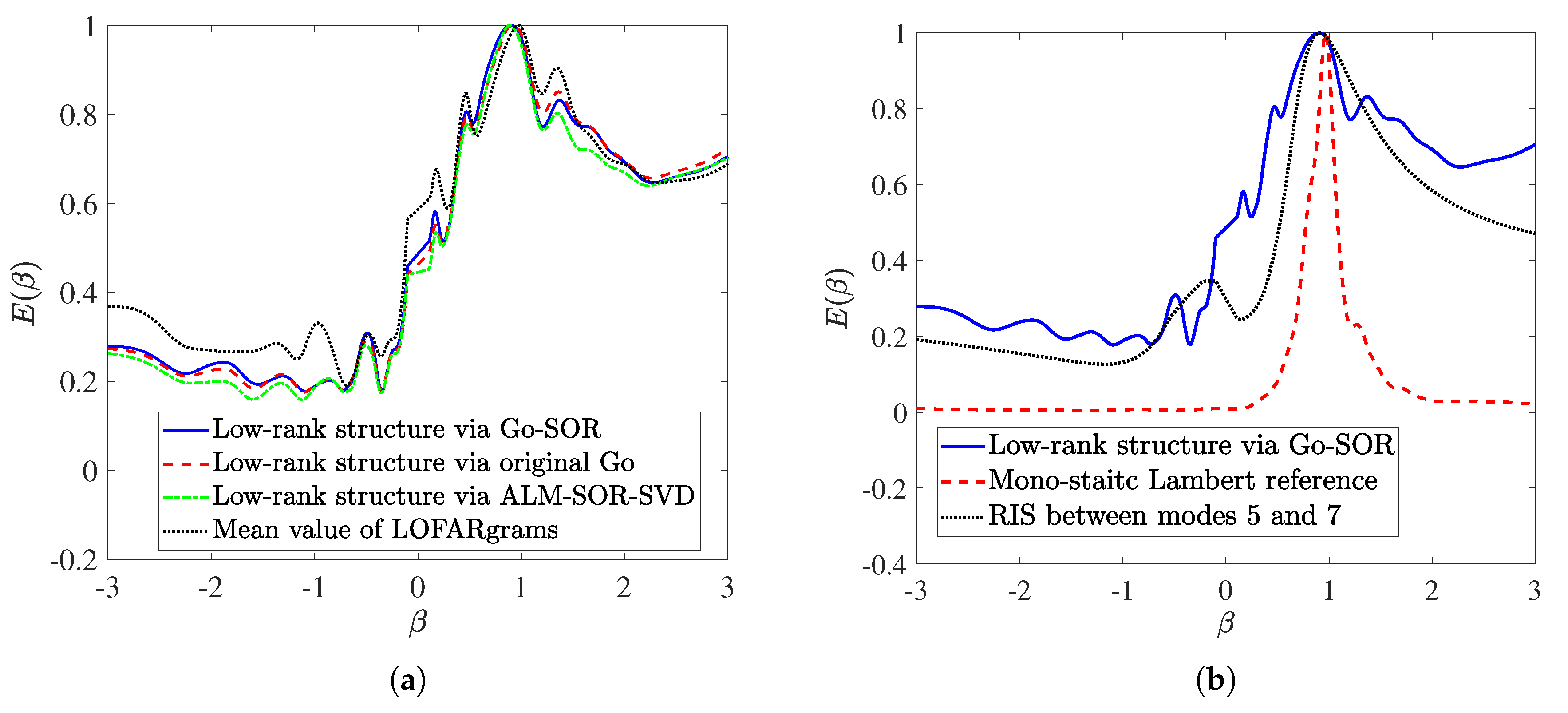
The corresponding distributions of RWIs in Figure 5 are shown in Figure 6a. The blue solid, red dashed, green dashed, and black dotted lines represent for the low-rank structure in Figure 5a (via Go-SOR), Figure 5b (via Go), Figure 5c (via ALM-SOR-SVD RPCA), and mean LOFARgram in Figure 5d, respectively. The curves show similar distributions of RWIs, indicating that the striation features of the four subfigures in Figure 5 are almost consistent. The coincidence of the peaks demonstrates the close values, making the processing of low-rank structure reverberations reliable.
4.2. Uniformity of RIS, Mean LOFARgram, and Low-Rank Structure
The contents in Figure 5 and Figure 6a illustrate the relationship between the RIS, mean LOFARgram, and low-rank structure, highlighting their uniformity.
For a simplified monostatic reverberation case in the experimental environment, the stochastic scattering amplitude in Equation (3) is assumed to be stationary, and the first and second moments exist [46]
Using Equation (8), the ensemble reverberation intensity element of intensity matrix with frequency index f and time index t can be expressed as follows:
where
Equations (16) and (17) show that the ensemble expression of stochastic reverberation loses randomness and is theoretically consistent with a certain Lambert reverberation with parameters and . In the experimental data treatment, the ensemble reverberation intensity is approximated by the mean LOFARgram of the Q () pings. Thus, we naturally obtain the following equation:
Therefore, the uniformity of the RIS (symbolizing the Lambert reverberation ) and mean LOFARgram is demonstrated. When considering a low-rank structure, the initialized condition in Go-SOR leads to the following relation:
which means that the low-rank structures of different ping numbers and are consistent. Another condition of the non-existence of a moving target implies
where is the zero matrix. Meanwhile, each ping of the reverberation intensity matrix can be written as
It can be observed that factorized terms and on the right-hand side (RHS) of Equation (21), which satisfy Equations (19) and (20), respectively, are unique. It is demonstrated that the low-rank structure obtained by the proposed algorithm is exactly the unique solution of the ensemble form of experimental RIS (mean LOFARgram ) under specific prior conditions. By combining these equations, the consistency between the low-rank structure and Lambert RIS can be theoretically established. Therefore, the RIS , mean LOFARgram , and low-rank structure are related by the following expressions:
4.3. Interference Properties of the Low-Rank Structure
Due to the influence of the time-varying environment, the interference properties of single-ping reverberation change sharply. As shown in Figure 5, obvious periodic interference phenomena can be observed in the low-rank matrices for multi-ping reverberation from 2 s to 4.5 s. By the uniformity of RIS and the low-rank structure, the interference frequency f of experimental data can be theoretically analyzed through Equation (16), which is the simplified monostatic model for shallow seabed reverberation.
The concept of interference frequency between modes m-th and -th is introduced to analyze the one-way process of bottom reverberation interference patterns:
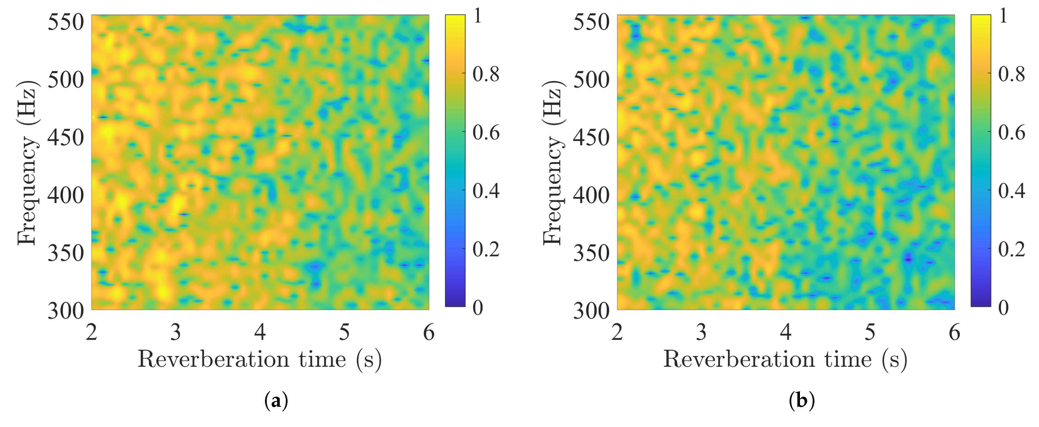
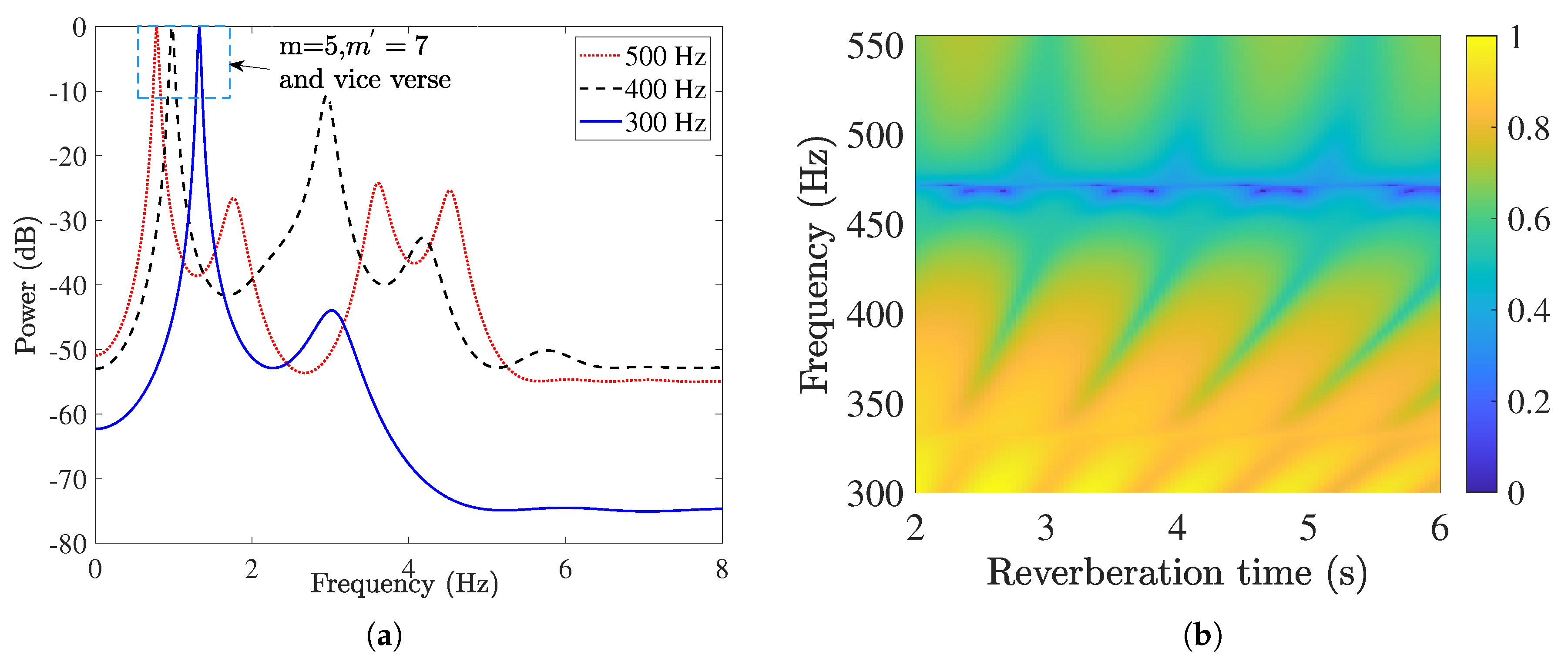
The dominant interference frequencies for the reverberation experimental data are determined through spectral analysis of the low-rank structure shown in Figure 5. For accurate frequency estimation, the reverberation intensity curves at different frequencies are detrended during pretreatment. We use the multiple signal classification (MUSIC) method to improve the resolution of estimated results [47]. The estimation of interference frequencies for the low-rank structure is shown in Figure 7a, where the blue solid line, black dashed line, and red dotted line represent the results of 300, 400, and 500 Hz, respectively. The frequencies corresponding to the highest peaks match the direct calculations of the fifth and seventh modes by Equation (23) under all three different frequencies.
The simulated fifth-and-seventh-only RIS, which is similar to the low-rank structure shown in Figure 5a between 2 s to 4.5 s, is described in Figure 7b. For comparison, distributions of the fifth-and-seventh-only RIS, monostatic Lambert RIS in Figure 3a, and low-rank structure in Figure 5a are described in Figure 6b, with the black dotted line, red dashed line, and blue solid line, respectively. We find that of the simulated fifth-and-seventh-only RIS matches well with the experimental low-rank structure. Because of the difference in the mode number in the simulation, the monostatic Lambert RIS, which is calculated under all modes, presents a more complex pattern compared to the fifth-and-seventh-only RIS, and the difference of in Figure 6b is apparent. The differences in the RWI corresponding to the peaks in Figure 6b are small enough, despite the deviation of the monostatic curve from the others. This demonstrates the conclusive control of the fifth and seventh modes in the experiment.
5. Discussion
In this study, we employed randomized separation algorithms to extract the low-rank structure of shallow seabed reverberation. We propose a modified Go-SOR decomposition method based on the equivalence of SOR-SVD and BRP, which exhibits superior comprehensive performance compared to the SOTA algorithm when processing low-frequency reverberation experimental data. We demonstrated the uniformity between the simulated Lambert RIS, low-rank structure reverberation, and ensemble intensity structure based on the simplified monostatic reverberation model. The spectral analysis of the low-rank structure reverberation and theoretical calculation of interference frequencies indicate that the interference structure is primarily controlled by the fifth and seventh modes in the experimental environment of the South China Sea.
The original contributions of this work are:
- A novel signal separation technique, named Go-SOR, was proposed and evaluated for processing reverberation experimental data. The results show that Go-SOR outperforms the SOTA algorithm ALM-SRO-SVD RPCA in terms of the computing time and definition index. Furthermore, we established the conditional equivalence of low-rank approximation between the SOR-SVD of the proposed algorithm and the BRP of the original Go algorithm.
- A bistatic low-frequency reverberation simulation model based on the normal mode theory was developed. When the transition indicator circular similarity is , the model can be transformed into a monostatic distant seabed reverberation model.
- The equivalence between the low-rank structure by the proposed algorithm and RIS was described, which provides the interpretability of the algorithm’s processing results. Our findings suggest that the study of RIS can be transformed into the study of the low-rank structure reverberation obtained from the data. This provides the possibility for the study of the data-driven RIS and other methods based on the data-driven RWI, and facilitates the acquisition of the dominant modes of the experimental sea area from the data.
The presented method has potential applications in seafloor exploration, RWI extraction, and active sonar dereverberation. Additionally, the proposed algorithm may facilitate the detection of strong moving targets by extracting sparse components and it may be a promising approach for detecting weak signals in the future.
Author Contributions
Conceptualization, J.P. and B.G.; methodology, J.P.; software, J.P.; validation, J.P. and B.G.; formal analysis, J.P. and B.G.; investigation, J.P.; resources, J.P. and B.G.; data curation, J.P.; writing—original draft preparation, J.P.; writing—review and editing, J.P. and B.G.; visualization, B.G.; supervision, B.G.; project administration, B.G.; funding acquisition, B.G. All authors have read and agreed to the published version of the manuscript.
Funding
This study was supported by the National Natural Science Foundation of China (CN) under grant number 11704359.
Data Availability Statement
Not applicable.
Acknowledgments
The authors thank Ning Wang for the insightful discussions and instructive guidance and Shutong Zong for the implementation of the MUSIC algorithm.
Conflicts of Interest
The authors declare no conflict of interest.
Appendix A. Calculation of E(β) by the Two-Dimensional Fourier Transform
To rigorously and accurately describe the slope information of the RIS, it is necessary to use the concept of the distribution of RWI. For a reverberation intensity matrix with a distance index and angular frequency index , a two-dimensional Fourier transform is performed on its mean-removal matrix
where the matrix can be written as in polar coordinates with the polar axis index K and angle index . According to Parseval’s theorem, is proven to be the energy distribution along the angle by Rouseff [35]
where B represents the truncated region of the polar axis K.
Appendix B. Equivalence of BRP- and SOR–SVD-Based Low-Rank Approximations
Assume a preset power scheme and oversampling parameter for the BRP (shown in Algorithm 1) and SOR-SVD (shown in Algorithm 2). Then, in BRP, we have the following:
Implementing the QR decomposition, we obtain
Thus, the low-rank approximation of rank r is expressed as follows:
where the term in (A5) is the projection matrix of and can be calculated using the QR decomposition (refer to Appendix C)
Substituting Equation (A6) into (A5), the low-rank approximation can be simplified as follows:
which is similar to the low-rank approximation of SOR-SVD in Algorithm 2. Considering the cases of and , the low-rank approximation in (A5) is revised to
Considering the SVD of , the SVD form of can be written as follows:
Indeed, and are the approximations of the order-r column and row space of [38], respectively. Refer to (A16), one obtains
where the subscripts indicate the first r columns of , and the superscripts indicate the unitary\orthogonal matrices. Taking (A9) and (A10) into (A8), we have
Following the same process, we have
Thus, we have
where the superscript of □ is ignored, except for that in .
Appendix C. The Proof of Equation (A6)
References
- Yang, S.E. Theory of Underwater Sound Propagation; Harbin Engineering University Press: Harbin, China, 2009. [Google Scholar]
- Holland, C.W.; Ellis, D.D. Clutter from non-discrete seabed structures. J. Acoust. Soc. Am. 2012, 131, 4442–4449. [Google Scholar] [CrossRef] [PubMed]
- Pang, J.; Gao, B.; Song, W.; Zuo, Y.; Mo, D. A Coupled Mode Reverberation Theory for Clutter Induced by Inhomogeneous Water Columns in Shallow Sea. In Proceedings of the 2021 OES China Ocean Acoustics (COA), Harbin, China, 14–17 July 2021; pp. 526–529. [Google Scholar] [CrossRef]
- Li, X.; Zhi, X. Research of underwater bottom object and reverberation in feature space. J. Mar. Sci. Appl. 2013, 12, 235–239. [Google Scholar] [CrossRef]
- Yu, G.; Piao, S. Multiple Moving Targets Detection and Parameters Estimation in Strong Reverberation Environments. Shock Vib. 2016, 2016, 5274371. [Google Scholar] [CrossRef]
- Yu, G.; Yang, T.C.; Piao, S. Estimating the delay-Doppler of target echo in a high clutter underwater environment using wideband linear chirp signals: Evaluation of performance with experimental data. J. Acoust. Soc. Am. 2017, 142, 2047–2057. [Google Scholar] [CrossRef]
- Zhu, Y.; Yang, K.; Duan, R.; Wu, F. Sparse spatial spectral estimation with heavy sea bottom reverberation in the fractional fourier domain. Appl. Acoust. 2020, 160, 107132. [Google Scholar] [CrossRef]
- Wall, M.E.; Rechtsteiner, A.; Rocha, L.M. Singular Value Decomposition and Principal Component Analysis. In A Practical Approach to Microarray Data Analysis; Springer: Boston, MA, USA, 2003. [Google Scholar]
- Huang, N.E.; Shen, Z.; Long, S.R.; Wu, M.C.; Shih, H.H.; Zheng, Q.; Yen, N.C.; Tung, C.C.; Liu, H.H. The empirical mode decomposition and the Hilbert spectrum for nonlinear and non-stationary time series analysis. Proc. Math. Phys. Eng. Sci. 1998, 454, 903–995. [Google Scholar] [CrossRef]
- Wu, Z.; Huang, N.E. Ensemble empirical mode decomposition: A noise-assisted data analysis method. Adv. Adapt. Data Anal. 2009, 1, 1–41. [Google Scholar] [CrossRef]
- Dragomiretskiy, K.; Zosso, D. Variational Mode Decomposition. IEEE Trans. Signal Process. 2014, 62, 531–544. [Google Scholar] [CrossRef]
- Schmid, P.J.; Sesterhenn, J. Dynamic mode decomposition of numerical and experimental data. J. Fluid Mech. 2010, 656, 5–28. [Google Scholar] [CrossRef] [Green Version]
- Zare, M.; Nouri, N.M. A novel hybrid feature extraction approach of marine vessel signal via improved empirical mode decomposition and measuring complexity. Ocean Eng. 2023, 271, 113727. [Google Scholar] [CrossRef]
- Fan, G.; Yu, P.; Wang, Q.; Dong, Y. Short-term motion prediction of a semi-submersible by combining LSTM neural network and different signal decomposition methods. Ocean Eng. 2023, 267, 113266. [Google Scholar] [CrossRef]
- Goldhahn, R.; Hickman, G.; Krolik, J.L. Waveguide Invariant Reverberation Mitigation for Active Sonar. In Proceedings of the IEEE International Conference on Acoustics, Honolulu, HI, USA, 15–20 April 2007. [Google Scholar]
- Goldhahn, R.; Hickman, G.; Krolik, J. Waveguide invariant broadband target detection and reverberation estimation. J. Acoust. Soc. Am. 2008, 124, 2841–2851. [Google Scholar] [CrossRef]
- Li, Y.Q.; Li, J.P.; Han, L. A Fast Sea Interface Reverberation Suppression Method Based on Unitary Transformation. In Proceedings of the 2010 International Conference on Digital Manufacturing and Automation, Changcha, China, 18–20 December 2010; Volume 1, pp. 3–6. [Google Scholar] [CrossRef]
- Xu, L.Y.; Liao, B.; Zhang, H.; Xiao, P.; Huang, J.J. Acoustic localization in ocean reverberation via matrix completion with sensor failure. Appl. Acoust. 2021, 173, 107681. [Google Scholar] [CrossRef]
- Kim, G.; Lee, K.; Lee, S. Linear Frequency Modulated Reverberation Suppression Using Non-negative Matrix Factorization Methods, Dechirping Transformation and Modulo Operation. IEEE Access 2020, 8, 110720–110737. [Google Scholar] [CrossRef]
- Jia, H.; Li, X. Underwater reverberation suppression based on non-negative matrix factorisation. J. Sound Vib. 2021, 506, 116166. [Google Scholar] [CrossRef]
- Candès, E.J.; Li, X.; Ma, Y.; Wright, J. Robust Principal Component Analysis? J. ACM 2011, 58, 1–37. [Google Scholar] [CrossRef]
- Zhou, T.; Tao, D. Godec: Randomized low-rank & sparse matrix decomposition in noisy case. In Proceedings of the 28th International Conference on Machine Learning, ICML 2011, Bellevue, WA, USA, 28 June–2 July 2011. [Google Scholar]
- Nie, R.; Liu, X.; Sun, C.; Zhou, Y. Multi-ping Reverberation Suppression Combined with Spatial Continuity of Target Motion. In Proceedings of the 2021 OES China Ocean Acoustics (COA), Harbin, China, 14–17 July 2021; pp. 689–693. [Google Scholar] [CrossRef]
- Liu, B.; Yin, J.; Zhu, G.; Guo, L. A target detection method in reverberation environment based on stochastic algorithm. J. Harbin Eng. Univ. 2020, 41, 277–281. [Google Scholar]
- Yin, J.; Liu, B.; Zhu, G.; Guo, L. A method of underwater target detection via nonnegative matrix factorization. In Proceedings of the 2019 IEEE International Conference on Signal, Information and Data Processing (ICSIDP), Chongqing, China, 11–13 December 2019; pp. 1–4. [Google Scholar] [CrossRef]
- Huang, H.; Zou, M.S.; Jiang, L.W. Study on the integrated calculation method of fluid-structure interaction vibration, acoustic radiation, and propagation from an elastic spherical shell in ocean acoustic environments. Ocean Eng. 2019, 177, 29–39. [Google Scholar] [CrossRef]
- Liu, J.Y.; Huang, C.F.; Shyue, S.W. Effects of seabed properties on acoustic wave fields in a seismo-acoustic ocean waveguide. Ocean Eng. 2001, 28, 1437–1459. [Google Scholar] [CrossRef]
- He, T.; Wang, B.; Mo, S.; Fang, E. Predicting range-dependent underwater sound propagation from structural sources in shallow water using coupled finite element/equivalent source computations. Ocean Eng. 2023, 272, 113904. [Google Scholar] [CrossRef]
- Song, H.; Cho, C.; Hodgkiss, W.; Nam, S.; Kim, S.M.; Kim, B.N. Underwater sound channel in the northeastern East China Sea. Ocean Eng. 2018, 147, 370–374. [Google Scholar] [CrossRef]
- Lepage, K.D.; Mcdonald, B.E. Environmental Effects of Waveguide Uncertainty on Coherent Aspects of Propagation, Scattering, and Reverberation. IEEE J. Ocean. Eng. 2006, 31, 413–420. [Google Scholar] [CrossRef]
- Grigor’ev, V.; Kuz’kin, V.; Petnikov, B. Low-frequency bottom reverberation in shallow-water ocean regions. Acoust. Phys. 2004, 50, 37–45. [Google Scholar] [CrossRef]
- Gao, B.; Pang, J.; Li, X.; Song, W.; Gao, W. Recovering reverberation interference striations by a conditional generative adversarial network. JASA Express Lett. 2021, 1, 056001. [Google Scholar] [CrossRef]
- Yu, S.; Liu, B.; Yu, K.; Yang, Z.; Kan, G.; Zhang, X. Comparison of acoustic backscattering from a sand and a mud bottom in the South Yellow Sea of China. Ocean Eng. 2020, 202, 107145. [Google Scholar] [CrossRef]
- Middleton, D. New physical-statistical methods and models for clutter and reverberation: The KA-distribution and related probability structures. IEEE J. Ocean. Eng. 1999, 24, 261–284. [Google Scholar] [CrossRef]
- Rouseff, D. Effect of shallow water internal waves on ocean acoustic striation patterns. Waves Random Media 2001, 11, 377. [Google Scholar] [CrossRef]
- Eckart, C.; Young, G. The approximation of one matrix by another of lower rank. Psychometrika 1936, 1, 211–218. [Google Scholar] [CrossRef]
- Johnson, W.B. Extensions of Lipschitz mappings into a Hilbert space. Contemp. Math. 1984, 26, 189–206. [Google Scholar]
- Halko, N.; Martinsson, P.G.; Tropp, J.A. Finding structure with randomness: Probabilistic algorithms for constructing approximate matrix decompositions. SIAM Rev. 2011, 53, 217–288. [Google Scholar] [CrossRef] [Green Version]
- Gu, M. Subspace iteration randomization and singular value problems. SIAM J. Sci. Comput. 2015, 37, A1139–A1173. [Google Scholar] [CrossRef] [Green Version]
- Kaloorazi, M.F.; de Lamare, R.C. Subspace-orbit-randomized decomposition for low-rank matrix approximations. IEEE Trans. Signal Process. 2018, 66, 4409–4424. [Google Scholar] [CrossRef] [Green Version]
- Fazel, M.; Candes, E.; Recht, B.; Parrilo, P. Compressed sensing and robust recovery of low rank matrices. In Proceedings of the 2008 42nd Asilomar Conference on Signals, Systems and Computers, Pacific Grove, CA, USA, 26–29 October 2008; pp. 1043–1047. [Google Scholar]
- Zhou, T.; Tao, D. Bilateral random projections. In Proceedings of the 2012 IEEE International Symposium on Information Theory Proceedings, Cambridge, MA, USA, 1–6 July 2012; pp. 1286–1290. [Google Scholar]
- Zhou, T.; Tao, D. Shifted subspaces tracking on sparse outlier for motion segmentation. In Proceedings of the Twenty-Third International Joint Conference on Artificial Intelligence, Citeseer, Beijing, China, 3–9 August 2013. [Google Scholar]
- Subbarao, M.; Choi, T.S.; Nikzad, A. Focusing Techniques. Opt. Eng. 1993, 32, 2824–2836. [Google Scholar] [CrossRef]
- Subbarao, M.; Tyan, J.K. Selecting the optimal focus measure for autofocusing and depth-from-focus. IEEE Trans. Pattern Anal. Mach. Intell. 1998, 20, 864–870. [Google Scholar] [CrossRef] [Green Version]
- Grimmett, G.; Stirzaker, D. Probability and Random Processes; Oxford University Press: Oxford, UK, 2020. [Google Scholar]
- Schmidt, R. Multiple emitter location and signal parameter estimation. IEEE Trans. Antennas Propag. 1986, 34, 276–280. [Google Scholar] [CrossRef] [Green Version]
Figure 2.
(a) SSP of the South China Sea. (b) Relative positions of the sources and receiver in the experiment.
Figure 2.
(a) SSP of the South China Sea. (b) Relative positions of the sources and receiver in the experiment.

Figure 3.
(a) Lambert RIS for mono-static case. (b) Lambert RIS for bi-static case. (c) Distributions of RWI for RISs in Figure (a,b).
Figure 3.
(a) Lambert RIS for mono-static case. (b) Lambert RIS for bi-static case. (c) Distributions of RWI for RISs in Figure (a,b).

Figure 4.
Experimental LOFARgrams for different reverberation pings. (a) Ping = 1. (b) Ping = 11. (c) Ping = 21. (d) Ping = 31.
Figure 4.
Experimental LOFARgrams for different reverberation pings. (a) Ping = 1. (b) Ping = 11. (c) Ping = 21. (d) Ping = 31.


Figure 5.
Reverberation intensity spectrum at a depth of 65 m. (a) Low-rank structure via Go-SOR decomposition. (b) Low-rank structure via Go decomposition. (c) Low-rank structure via ALM-SOR-SVD RPCA decomposition. (d) The mean value of 31 ping LOFARgrams.
Figure 5.
Reverberation intensity spectrum at a depth of 65 m. (a) Low-rank structure via Go-SOR decomposition. (b) Low-rank structure via Go decomposition. (c) Low-rank structure via ALM-SOR-SVD RPCA decomposition. (d) The mean value of 31 ping LOFARgrams.

Figure 6.
(a) Distributions of RWI corresponding to the sub-figures shown in Figure 5. (b) Distributions for the comparison of processed and simulated results.
Figure 6.
(a) Distributions of RWI corresponding to the sub-figures shown in Figure 5. (b) Distributions for the comparison of processed and simulated results.

Figure 7.
(a) Estimations of interference frequencies for the low-rank structure, and the peaks indicate that the low-rank structure is controlled by the fifth and seventh modes significantly. (b) RIS consists of the fifth and seventh modes in the simulation.
Figure 7.
(a) Estimations of interference frequencies for the low-rank structure, and the peaks indicate that the low-rank structure is controlled by the fifth and seventh modes significantly. (b) RIS consists of the fifth and seventh modes in the simulation.


Table 1.
SSIM of every two different reverberation pings.
| Ping Number | 1 | 11 | 21 | 31 |
|---|---|---|---|---|
| 1 | - | 0.0845 | 0.1396 | 0.1030 |
| 11 | 0.0845 | - | 0.1002 | 0.0860 |
| 21 | 0.1396 | 0.1002 | - | 0.1080 |
| 31 | 0.1030 | 0.0860 | 0.1080 | - |
Table 2.
Reverberation data processing times for , , and .
| Algorithms | Go-SOR | Original Go | ALM-SOR-SVD RPCA |
|---|---|---|---|
| Computing time (s) | 0.44 | 55.20 | 0.76 |
Table 3.
Normalized definition indices of the low-rank structure reverberation via different algorithms.
Table 3.
Normalized definition indices of the low-rank structure reverberation via different algorithms.
| Go-SOR | Original Go | ALM-SOR-SVD RPCA | |
|---|---|---|---|
| EOG | 1 | 0.8352 | 0.9100 |
| Tenengrad | 1 | 0.8398 | 0.9304 |
| Brenner | 1 | 0.7472 | 0.6825 |
| Laplacian | 1 | 0.8406 | 0.8974 |
Disclaimer/Publisher’s Note: The statements, opinions and data contained in all publications are solely those of the individual author(s) and contributor(s) and not of MDPI and/or the editor(s). MDPI and/or the editor(s) disclaim responsibility for any injury to people or property resulting from any ideas, methods, instructions or products referred to in the content. |
© 2023 by the authors. Licensee MDPI, Basel, Switzerland. This article is an open access article distributed under the terms and conditions of the Creative Commons Attribution (CC BY) license (https://creativecommons.org/licenses/by/4.0/).
Share and Cite
MDPI and ACS Style
Pang, J.; Gao, B. Application of a Randomized Algorithm for Extracting a Shallow Low-Rank Structure in Low-Frequency Reverberation. Remote Sens. 2023, 15, 3648. https://doi.org/10.3390/rs15143648
AMA Style
Pang J, Gao B. Application of a Randomized Algorithm for Extracting a Shallow Low-Rank Structure in Low-Frequency Reverberation. Remote Sensing. 2023; 15(14):3648. https://doi.org/10.3390/rs15143648
Chicago/Turabian StylePang, Jie, and Bo Gao. 2023. "Application of a Randomized Algorithm for Extracting a Shallow Low-Rank Structure in Low-Frequency Reverberation" Remote Sensing 15, no. 14: 3648. https://doi.org/10.3390/rs15143648
Note that from the first issue of 2016, this journal uses article numbers instead of page numbers. See further details here.