


Fast SAR Image Simulation Based on Echo Matrix Cell Algorithm Including Multiple Scattering
Institute of Geospatial Information, Information Engineering University, Zhengzhou 450001, China
*
Author to whom correspondence should be addressed.
Remote Sens. 2023, 15(14), 3637; https://doi.org/10.3390/rs15143637
Submission received: 7 May 2023
/
Revised: 16 July 2023
/
Accepted: 18 July 2023
/
Published: 21 July 2023
(This article belongs to the Special Issue Modeling, Processing and Analysis of Microwave Remote Sensing Data)
Abstract
:We present a novel fast synthetic aperture radar (SAR) image simulation method based on the echo matrix cell algorithm including multiple scattering. To improve the efficiency of SAR image simulation while ensuring the fidelity of the simulated results, we first discretized the target facets set in the SAR beams footprint into lattice targets using the range-Doppler (RD) imaging geometry model and provided the basis for simulating electromagnetic wave transmission. Based on the simulation of electromagnetic waves transmission, we used the ray tracing algorithm to calculate the multiple backscattering field including multi-polarimetric information and various material properties. Then, based on the echo matrix cell algorithm, we set the echo matrix cell as the subfield of the target backscattering field and designed the CUDA kernel function to implement a computation parallelization for SAR echo generation. All the echo matrix cells are traversed in parallel to obtain the total backscattering field of the target, reproducing the time-varying characteristic of the backscatter coefficient for each lattice target within the synthetic aperture time. The echo signal is processed using the RD imaging algorithm to obtain the simulated SAR image. Finally, we select some targets including aircraft carrier and airplane models for simulation tests. The computation efficiency is improved over 170-fold by comparing the computations of the proposed method and CPU single-thread. We also performed some qualitative and quantitative evaluations on the fidelity of the simulated SAR images. The experimental results verify the effectiveness of the proposed method.
1. Introduction
Synthetic aperture radar (SAR) is an active high-resolution imaging sensor that has played a great role in both military and civilian applications. Since the real image data obtained from SAR are limited to meet the actual demands, the development of SAR image simulation technology has been promoted. Echo-based SAR image simulation can reproduce the actual working process from the transmitting end to the receiving end of the radar sensor, and it has become a powerful tool for establishing target datasets [1,2,3]. At present, echo-based SAR image simulation is becoming more practical, the fidelity of the simulation results is demanded to be higher, and its computational load is also increasing sharply. Therefore, it is a critical issue to effectively improve the efficiency of SAR echo simulation while ensuring the fidelity of the simulation results. Recently, many studies on fast echo-based SAR image simulation have been conducted.
According to the ways of obtaining the backscatter coefficient, these studies can be roughly divided into two categories: inverse simulation methods and forward simulation methods. Most studies on the inverse simulation methods simplify the process of obtaining the backscatter coefficient to improve the efficiency of simulation. Some studies do not consider multiple scattering and usually directly use SAR magnitude images as backscattering coefficients to participate in echo simulations, and many acceleration methods have been proposed. Some studies have proposed representative GPU-accelerated simulation methods that effectively solve the high computational load problem of SAR echo simulation with the help of the CUDA platform. Wang et al. proposed a fast echo simulation and imaging method, which simulated the azimuthal signal at the GPU device side and the distance signal at the CPU host, and quickly obtained the target echo signal and the simulated images [4]. Zhang et al. proposed a CUDA-based method for the raw data simulation of interferometric synthetic aperture radar (InSAR). The simulation efficiency was greatly improved by using thousands of threads to execute multiple sub-scene tasks in parallel [5]. Zhu et al. proposed an efficient missile-carrying SAR raw echo signal simulation method. A multi-threaded parallel program using a GPU was used to simulate each data block, which greatly speeds up the simulation of the raw echo signal [6]. Chen et al. proposed an airborne bistatic SAR echo simulation algorithm based on CUDA architecture. The CPU multi-threads were used to control the multi-GPUs platform for echo simulation, which improves the speed of SAR echo simulation [7]. Sheng et al. proposed a fast echo simulation method for complex scenes, calling each thread of the GPU to be responsible for the echo simulation of a single scattering unit, but the backscatter coefficient was set in advance [8,9]. Yu et al. proposed a GPU-based Circular Synthetic Aperture Radar echo simulation method to improve the simulation efficiency of large scenes, and simplified the backscatter coefficient calculation process [10]. Zhang et al. introduced a multi-GPUs method for accelerating time–domain SAR raw data simulation, which had a good acceleration simulation effect on wide and high-resolution SAR raw data [11]. Xu et al. adopted the one-dimensional frequency domain Fourier transform algorithm to design a SAR real-time echo simulator based on multi-FPGA parallel computing. The validity of the SAR echo simulator had been verified by the imaging results of lattice targets [12]. A SAR echo simulation method with complementary advantages of GPU and CPU is designed, which improved the efficiency of echo simulation [13]. Zhang et al. improved the computational power by integrating cloud computing and GPU based on the multi-modal decomposition method of the stripmap model to simulate GF-3 raw data [14].
Compared with the inverse simulation methods, the forward simulation methods can reproduce the actual working process of SAR and simulate the entire propagation process of electromagnetic waves from the transmitting end to the receiving end. Forward simulation methods are mainly concerned with how the radar wave interacts with the target and focus more on the real process for obtaining the target backscattered field. The essence of this category of methods is the simulation of SAR imaging mechanism, which has great practical value. Franceschetti’s team has proposed some representative series of methods for fast echo simulation in the frequency domain, focusing on the fast echo simulation of large scenes. The frequency domain simulation method transforms complex convolution in the time domain into a frequency domain multiplication, and enables the echo simulation of large scenes in a highly time-efficient way. An advanced SAR simulator (SARAS) was designed to calculate the target backscatter coefficient using the Kirchhoff approximation, multiply it with the SAR impulse response in the frequency domain, and then obtain the SAR raw echo data quickly using a two-dimensional inverse Fourier transform [15,16,17]. A SAR echo and image simulation method for use on the ocean surface was proposed; the sea surface was modeled using a distributed surface model, and the correctness of the method was verified by analysis of the wave SAR image spectra [18,19]. A method for spotlight SAR echo simulation for extended scenarios was proposed, which can greatly speed up the echo simulation with the help of fast Fourier transform [20,21]. A SAR echo simulation method for urban scenes is proposed, which uses the Kirchhoff approximation to calculate the backward scattering coefficients of each component including multiple scattering [22]. However, the above frequency domain simulation methods cannot meet the current demand for image-oriented mechanistic simulations, mainly at the expense of phase accuracy and ignoring the detailed processes of the actual interaction between electromagnetic waves and targets. In addition to the forward simulation methods based on the small surface facets theory, there are also forward simulation methods based on the electromagnetism theory and the physical illumination model theory. Dong et al. proposed an improved ray tracing algorithm and combined it with the GO-PO/-PTD algorithm to improve the computational efficiency of the composite scattered field of a 3D ship target and the sea surface [23]. The multiple scattering echo simulation and imaging experiments based on CUDA were carried out using the shooting bouncing ray (SBR) method, which improved the efficiency and fidelity of the simulations [24]. Wu et al. proposed a novel echo-based SAR image simulation method that comprehensively utilizes both SAR effective view and ray tracing algorithms, and improved the fidelity of simulated SAR images [25]. Drozdowicz et al. improved the illumination model according to the working mechanism of SAR and proposed an open-source SAR echo simulator in combination with ray tracing algorithm, which achieved better simulation results [26]. Wei et al. combined the time–domain shot and bounced ray (TD-SBR) method with time–domain physical optics (TD-PO) to develop a high-frequency simulation tool that can quickly obtain backscatter echo from large complex targets [27]. Kee et al. proposed an efficient GPU implementation of the high-frequency SBR-PO method. This method significantly reduced the computational time required for modeling the backscattering of electrically large and arbitrarily shaped objects, and provided a new solution for improving the efficiency of SAR image simulation [28]. Forward simulation methods focus on the real process of backscattering between electromagnetic waves and targets, and some relevant representative studies have also proposed well-built backscattering modeling methods. Auer et al. carried out a simulation study of high-resolution SAR images by improving the illumination model using the ray tracing algorithm to map the 3D scene to the SAR slant range coordinate system [29,30]. Some studies have built some backscattering models using ray tracing with the help of the CUDA platform to carry out experiments on the multiple scattering energy tracking of scenes in the SAR slant range coordinate system [31,32,33]. Such studies usually obtain SAR simulation images with clear texture and high timeliness, which are convenient for establishing SAR target datasets. This series of methods does not involve the echo generation and imaging process, but also provides new ideas for echo-based SAR image simulation studies.
The above studies have achieved good results in fast SAR image simulation, but most of the proposed acceleration architectures are designed for specific echo simulation scenarios, sacrificing the fidelity of the backscatter coefficient, and do not have good generalizability and practicality. So, there is an urgent demand to design a fast SAR image simulation method under the prerequisite of ensuring the high fidelity of simulation results. At present, with the development of high-resolution SAR systems, the synthetic aperture time is growing longer and the Doppler bandwidth is becoming larger, and the backscatter coefficient of the target has certain time-varying characteristic within the corresponding synthetic aperture time. Especially for scenes with complex structures, the fixed scattering center assumptions can affect the fidelity of the echo simulation. In addition, some studies have carried out some SAR echo simulations based only on the single scattering of electromagnetic waves. Practically, the electromagnetic waves transmitted by radar undergo multiple scattering with the target surface, and the multiple scattering magnitude and phase of the target are also obtained dynamically in real time. To handle the above issues, some representative studies proposed some high or low frequency approximation methods such as SBR and MOM to obtain the backscatter coefficient of the target, and then used the CUDA platform to perform echo simulation and obtain the simulated image after the echo signal’s focus processing. These studies simultaneously improved the efficiency and fidelity of SAR image simulation, but still adopted the assumption of a fixed backscattering center. In addition, most of these studies utilized commercial electromagnetic scattering software, and the fixed data format prevented further optimization of the algorithms. Some studies separated the magnitude and phase for simulation, and did not fully reproduce a real-time dynamic record of the magnitude and phase of multiple backscattering. The acceleration architectures related to the above studies are not generalizable, and are mostly applicable only under the assumption of a fixed backscattering center or known backscattering coefficient of the target. In summary, there is still an urgent demand to design a fast SAR image simulation method under the prerequisite of ensuring the fidelity of the simulation results.
To address the aforementioned limitations, this paper proposes a novel fast SAR image simulation method based on the echo matrix cell algorithm. We first used the RD imaging geometry to build the target latticing model, and provided a new solution for simulating the transmission of electromagnetic waves accurately. On the basis of the simulation of electromagnetic waves transmission, we used the ray tracing algorithm to calculate the multiple backscattering field including full-polarization information and various target surface material properties. Based on the echo matrix cell algorithm, we designed an efficient CUDA kernel function and gridded the total global backscattering field of the target with the help of the SAR spatial traversal idea and phase reference system characteristics. The CUDA-based platform calls GPU multithreads to traverse the full cells of the target echo matrix in parallel to rapidly obtain the total backscattering field of the target, fully reproducing the time-varying characteristics of the backscatter coefficient within the corresponding synthetic aperture time of the target. The target echo signal is processed using the RD imaging algorithm for 2D compression and to obtain the simulated SAR focused image.
The main contributions of this paper are as follows:
- A simulation method of electromagnetic waves transmission is designed to provide the basis for calculating the multiple backscattering field. The method mainly utilizes the RD imaging geometry and combines the lattice targets in the beam footprint with the radar real-time position to simulate the electromagnetic waves transmission;
- A calculation method of the multiple backscattering field is proposed to reproduce the time-varying characteristic of the target backscatter coefficient within the synthetic aperture time. The method mainly uses the ray tracing algorithm to track the multiple scattering paths of electromagnetic waves, including multi-polarimetric information and various material properties;
- A novel echo-based fast SAR image simulation method including multiple scattering is proposed to improve the efficiency of SAR image simulation while ensuring the high fidelity of the simulated results. The method uses the echo matrix cell algorithm to design the effective CUDA kernel function and quickly obtain the target backscattering field including multiple scattering.
This paper is organized as follows: Section 2 introduces the simulation of electromagnetic wave transmission and the calculation of the multiple backscattering field. Based on the echo matrix cell algorithm, Section 3 introduces a design of the CUDA kernel function. Section 4 verifies the effectiveness of the proposed method based on objective analysis and a comparison of the experimental results. Section 5 presents the conclusions.
2. Calculation of the Multiple Backscattering Field Using the Ray Tracing Algorithm
The calculation task of the multiple backscattering field is focused on the real-time dynamic recording of the magnitude and phase of multiple scattering between electromagnetic waves and target. We first used RD imaging geometry to discretize the target model surface facets within the radar beam footprint into lattice targets, and then by combining these with the real-time transmitting position of the radar platform, the directions of the electromagnetic wave transmission can be accurately determined. Based on the simulation of electromagnetic waves transmission, according to the light-like nature of microwaves, we chose the standard illumination model as the base scattering model and improved it comprehensively. Multiple scattering paths are traced for each discrete electromagnetic wave using the ray tracing algorithm, and the multiple scattering magnitude and phase are recorded dynamically in real time. The propagation distance decay factor is added according to the effect of propagation distance on the attenuation of echo energy in the radar equation. We combined the polarimetric scattering theory and the small perturbation method to obtain multi-polarimetric information for each backscattering of the electromagnetic wave. In short, the calculation of the multiple backscattering field can provide the basic conditions for SAR echo simulation, and serve as the key technical support for fast echo-based SAR image simulation using the CUDA platform.
2.1. Simulation of Electromagnetic Waves Transmission
When simulating radar beams moving along the azimuth direction and scanning a scene in the computer virtual environment, large numbers of electromagnetic waves are transmitted. The key point to ensure the high fidelity of SAR simulation images is to accurately calculate incidence directions of the electromagnetic waves. In order to ensure the calculation accuracy of the transmitted directions of the electromagnetic waves, we used the RD imaging geometry theory. The target model facets in the SAR beam footprint are discretized into lattice targets, and the initial transmitted position of the electromagnetic waves can be obtained according to the preset trajectory of the radar sensor along the azimuth direction. The incidence directions of electromagnetic waves can be determined effectively by combining the lattice targets with the moving positions of the radar sensor. In addition, target latticing also provides the preconditions for calculating the multiple backscattering field using the ray tracing algorithm and the judgment of radar beam footprint and shaded areas.
The essence of target latticing is the process of reasonably eliminating invalid facets in shaded areas and finely subdividing the effective facets in the beam footprint. As is shown in Figure 1, we first used the RD imaging geometry as the geometric basis to build the target latticing model. The center section of the radar beam is scanned along the azimuth time axis. When the squint angle is zero, the center section of the radar beam can be considered as the plane of zeros Doppler, as shown in the plane STA in Figure 1. The scan mode using the plane of zeros Doppler can meet the accuracy requirements for low- or medium-resolution SAR image simulation under the plane wave approximation. As the requirements related to SAR simulation image resolution increase, the synthetic aperture time grows longer and the Doppler bandwidth becomes larger, the scan mode using the plane of zeros Doppler will produce errors at the boundary between the beam footprint and the shaded areas.
In order to improve the accuracy of high-resolution SAR image simulation, referring to Figure 1, we refined the incidence directions of discrete electromagnetic waves within the synthesized beamwidth, and used the section of real-time beam edge along the azimuth direction to scan the scene, as shown in the plane STB in Figure 1. We needed to rotate the incidence directions of all discrete electromagnetic waves in the plane of zeros Doppler by an angle around the vertical axis ST in the stripmap SAR mode. Point changes to point B after the rotation of the plane of zeros Doppler to the beam edge. If the squint angle is zero, the rotation angle should be half of the synthesized beamwidth. If the radar squint angle is set, the rotation angle should be corrected to the sum of the squint angle and half of the synthesized beamwidth.
where refers to the real-time incidence directions within the plane STB. is the real-time incidence directions within the plane of zeros Doppler. is the rotation angle. is the synthesized beamwidth. is the radar squint angle. is the azimuth beamwidth, is the wavelength, and is the azimuth antenna size.
Then, we further gridded the scene based on the target latticing geometric model in Figure 1. The number of rows and columns in the scene grids are related to the sampling interval, and the setting of the lattice intervals follows Nyquist’s sampling law. In the actual tests, the lattices interval is one third of the SAR system resolution required to satisfy the Nyquist’s sampling law, and to avoid excessive subdivision of the model facets and reduce the complexity of calculating the multiple backscattering field using the ray tracing algorithm. We set the scene center as the origin of the coordinate system, and the number of rows and columns can be expressed as
where is the number of azimuth rows and is the number of range columns. is the azimuth resolution and is the slant range resolution. is the minimum azimuth coordinate in the scene and is the maximum azimuth coordinate in the scene. is the near slant range and is the far slant range. is the platform height. is the near ground range in the scene and is the far ground range coordinate in the scene. is the incidence angle. We transmitted discrete electromagnetic waves line by line along the azimuth direction, and the real-time position of the sensor can be written as
where S are the real-time positions of the sensor. refers to the azimuth coordinates of the sensor and i is the index of azimuth rows. The decomposition of the incidence vector of the electromagnetic wave within the plane of zeros Doppler is zero along the azimuth direction. We divided the size of each range gate according to the preset sampling interval, and then inversed to obtain the incidence direction of each discrete electromagnetic wave from near range to far range by each range gate. The incidence directions of the discrete electromagnetic waves are accurately calculated by the radar platform height and the changing angles among the slant ranges within the plane of zeros Doppler. The incidence directions of the electromagnetic waves within the plane of zeros Doppler are then rotated around the vertical axis ST to the section of real-time beam edge along the azimuth direction. The above is the basic preparation for simulating SAR beams scanning, and the specific process can be expressed by Equation (4)
where j is the index of range columns. is the real-time slant range according to slant range resolution. and are the adjacent incidence angles. is the incidence direction. is the squint angle of the beam center in the linear geometry, measured from the plane of zero Doppler.
Combining Equations (3) and (4), we scanned the scene with the section STB of the edge of the radar beams and simulated large numbers of discrete electromagnetic waves transmitting into the scene. Each discrete electromagnetic wave needs to traverse the whole model facets set, and obtain the propagation distance from the sensor to the intersected facet. The propagation distance can be obtained through the geometric relationship among the intersection point, the sensor position, the incidence direction, the normal vector of the surface facets, and one point on the surface element using Equation (5).
where P is the intersection point coordinate. S is the real-time position of the sensor, and t is the propagation distance from S to P. is the normal vector of the facet. is a random vertex point of the facet. When each electromagnetic wave intersects with the target model, the number of intersected facets may be more than one. We selected the facet at the minimum of t as the illuminated facet in the beam footprint, and the boundary between the beam footprint and the shadow area could thus be determined. Finally, we obtained the coordinates of the intersection points and accurately discretized the facets in the beam footprint into lattice targets.
The target model is scanned using the target latticing model, as shown in Figure 2. The dual-scale subdivision idea is also adopted in the process of target latticing, with large surface facets for planar parts and small surface facets for curved parts of the target model. During the whole process of target latticing, the target model still maintains the dimensions of irregular facets and does not uniformly subdivide all facet edges to the wavelength scale. To a certain extent, it can effectively avoid the excessive subdivision of the model facets and reduce the complexity of calculating the multiple backscattering field using the ray tracing algorithm in Section 2.2.
After the lattice targets are obtained, as shown in Figure 3, large numbers of electromagnetic waves can be simulated and transmitted into the scene by combining the real-time position of the sensor and the coordinates of the lattice targets. This simulation method can make the incidence directions of electromagnetic waves within the radar beamwidth more refined and overcome the defect of beam pointing ambiguity under the plane wave assumption. The task of electromagnetic wave transmission can be expressed by Equation (6).
where are the incidence directions and are the electromagnetic waves transmitting into scene. S are the real-time positions of the sensor. P are the coordinates of the lattice targets.
The above simulation of electromagnetic waves transmission is based on the RD imaging geometry model. It can effectively determine the SAR beam footprint and shadow areas, and discretize the target model surface facets in the radar beams footprint into lattice targets. The method strictly follows the real working mechanism of SAR, which can improve the certainty and accuracy of the incidence directions for transmitting electromagnetic waves. We propose the above electromagnetic wave transmission simulation method mainly to further provide key technical support for calculating the multiple backscattering field using the ray tracing algorithm shown in Section 2.2.
2.2. Calculation of the Multiple Backscattering Field
Based on the simulation of electromagnetic wave transmission, we can start to calculate the multiple backscattering field of the target. During the propagation of the microwave, when hitting a target of electronically large size, it will be reflected and has the nature of a light wave. In other words, the shorter the wavelength of the microwave is, the more similar its propagation nature is to geometric optics. In addition, in the derivation of the physical optics (PO) equation, we find that the key variable for calculating the backscattering field of the target facet is the angle between the incident direction of the electromagnetic wave and the normal vector of the target facet, and the rest of the parameters are auxiliary. The physical illumination model can be described comprehensively as the function of the angle between the incident direction of the electromagnetic wave and the normal vector of the facet, the angle between the normal vector of the facet and the received direction, the facet’s material properties, multi-polarimetric information and the target backscattering amplitude. Advanced RaySAR software also uses this backscattering model [29,30], which has a strong algorithmic inclusion. Therefore, we chose the standard illumination model as the base scattering model, and comprehensively improved it by using the ray tracing algorithm, radar equation and the polarimetric scattering theory. At the same time, we also considered that there are some variations in the initial incidence direction and propagation period of each discrete electromagnetic wave transmitted for each lattice target at the corresponding synthetic aperture time, which makes the backscatter coefficient of each lattice target more time-variable.
Each discrete electromagnetic wave is the basic unit being processed directly in the process of obtaining the total backscattering field for the whole target. We first focused on calculating the magnitude and phase of the backscatter coefficient of each discrete electromagnetic wave. The obtained magnitude and the phase of the multiple backscattering are vectors superimposed as the backscattering field of each discrete electromagnetic wave. The backscattering fields of all the discrete electromagnetic waves transmitted into the scene are vector-superimposed as the total backscattering field of the whole target.
The specific processes of calculating the multiple backscattering field of the target are as follows.
Firstly, we adopted the “go–stop” mode as the geometric basis for the SAR sensor to receive and transmit electromagnetic waves. The entire backscatter model has only one unique radiation source, and the exact location of the radiation source is determined by the coordinates of the radar sensor moving in real time along the azimuth. The “go–stop” mode can meet the airborne SAR echo simulation accuracy requirements, and the SAR sensor transmits discrete electromagnetic waves to the scene to be simulated sequentially along the azimuth time axis. The linear frequency modulation signal transmitted by radar can be written as
where is the pulse duration and is fast time along the range direction. is the range frequency modulation rate and is the carrier frequency. is the rectangular envelope. The echo signal can be given by
where is the real-time slant range from the sensor to the point target. is the slow time along the azimuth direction. The real-time changes of can generate the Doppler frequency history. The response signal after demodulation can be written as
where is the range envelope and is the range phase. is the azimuth envelope and is the Doppler phase. When designing the CUDA kernel function in Section 3.1, the two-dimensional (2D) envelopes can constrain and filter the lattice targets in real time. After adopting this “go–stop” mode, the PRF and range sampling rate need to be set reasonably to ensure the performance of range and azimuth ambiguities. It is usually required that the PRF of the radar system is more than 1.1 times the Doppler bandwidth , and the pulse repetition period is greater than the ground scene delay corresponding to the 3db range beamwidth. Therefore, the PRF should satisfy the constraint given by the following Equation (10):
The platform speed of airborne SAR is usually low, and we can set the PRF to about 1.4 times the azimuth bandwidth for improving the SAR SNR in our tests.
Secondly, we combine the real properties of the non-transparent material of the target to be simulated. The types of electromagnetic wave interaction with the target surface are fully considered in the tests, including specular reflection, subsurface reflection, diffuse reflection and absorption, not including refraction and transmission [34,35,36,37]. The parameters of the target material properties include specular reflection coefficient, specular reflection index, relative permittivity, diffuse reflection coefficient and energy decay coefficient, while ensuring the fidelity of the target backscatter coefficient obtained using the ray tracing algorithm. According to the quantitative relationship between electromagnetic wave propagation distance and echo energy in the radar equation, the fourth power of the real-time propagation distance is taken as the distance decay factor. The multiple backscattering field of each discrete electromagnetic wave can be expressed by Equation (11).
where represents the multiple backscattering field of each electromagnetic wave, which also points out that obtaining the magnitude and phase of multiple scattering is the key to the whole simulation test. is the magnitude at the k-th scattering, which is a complex function of the target material properties and propagation distance, followed by a detailed derivation process. is the phase at the k-th scattering, which is related to the real-time slant range and contains both range and Doppler phase. K is the total number of scatterings. is the diffuse reflection coefficient and is the specular reflection coefficient. is the relative permittivity of the target material. is the specular reflection index. is the fourth power of the real-time propagation distance. is the energy decay coefficient.
Referring to Figure 4, it should be noted that during the process of tracing the multiple scattering paths of electromagnetic waves, the types of interacted model parts are changing, so the material properties and normal vectors of the intersected surface facets are constantly changing, and the energy and polarimetric states of the electromagnetic waves are also changing in real time. The surface material of each target part is the composite with a certain gloss and roughness, and specular and diffuse reflections energy are the main components of the target backscatter energy. In fact, the diffuse and specular reflection components are derived from the microsurface theory. When the normal vectors of micro facets are more disordered, it means the anisotropy index of micro facets is larger and the target surface is macroscopically rougher, meaning the scattered energy at the intersection between electromagnetic waves and the target surface will be scattered in all directions. On the contrary, when the normal vectors of micro surface facets are more orderly, it means the scattered energy at the intersection between electromagnetic waves and the target surface will be concentrated along the specular reflection direction. Combined with the actual physical properties of the target surface material, reasonable adjustments of the material parameters can control the anisotropy index of the normal vectors of the micro facets.
Therefore, in the process of calculating the energy of diffuse and specular reflection, we comprehensively consider the effects of the surface material properties of each model part, the variable polarization of electromagnetic waves and the propagation distance on the backscatter magnitude. In addition, we highlight the comprehensive effects of two key angles on the backscattering magnitude when multiple scattering occurs; one is the angle between the incidence direction and the facet normal vector, and the other is the angle between the reflection direction and the receiving direction. Based on the actual scattering mechanism of electromagnetic waves with the target surface and the polarization principle, we designed the magnitude model of multiple backscattering, and the in Equation (11) can be expressed by Equation (12). It is worth noting that some key variables of the magnitude model are preset here, followed by a detailed derivation process, mainly used to illustrate the logic of building the model.
where is the backscatter energy at the k-th scattering. is the forward incident energy at the k-th scattering. is the initial value of the electromagnetic wave energy.
is the magnitude of the k-th scattering. is the real-time slant range at the k-th scattering. represents the mechanism of diffuse energy scattering in all directions. is the k-th polarimetric reflection coefficient, which is related to the material permittivity and the local incidence angle, followed by a detailed derivation process. is the receive direction from the intersection point to the real-time sensor position . is the distance from scattering intersection to . is the distance from the k-th intersection point to the real-time sensor position .
Based on the above analysis, real-time calculations of the forward incident energy, time-varying propagation direction, reflection direction and intersection coordinates, propagation distance is the key to calculating the multiple backscattering field. The electromagnetic wave follows the law of the conservation of energy during the process of multiple scattering, and the propagation energy continues to decay. As shown in Figure 4, each electromagnetic wave intersects with different model parts, and the material properties of each part of the facets are different and have different effects on the propagation energy decay. We set the energy decay threshold in tests to effectively prevent electromagnetic waves from entering dead loops when they hit the cavity structure. The energy decay during the process of multiple scattering can be represented by Equation (13)
where is set to 1.0 as the initial value of the electromagnetic wave energy. is the energy decay coefficient of the model facets. is set to 0.1 as the energy threshold value. Setting the energy decay threshold also allows for the self-judgment termination of tracking for each of the complex multiple scattering paths of discrete electromagnetic waves.
The essence of simulating multiple scattering is to simulate the process of the iterative propagation of electromagnetic waves. The ray tracing algorithm is mainly used to implement the tracing of multiple scattering paths for electromagnetic waves. The specular reflection direction and intersection coordinates of the electromagnetic wave at the -th scattering are used as the new incidence direction and new transmitted position of the electromagnetic wave at the k-th scattering, respectively. Therefore, we need to accurately calculate the specular reflection direction and the intersection coordinates with the target surface at each scattering of electromagnetic waves, completing the next round of scattering simulations of electromagnetic waves. Based on the simulation of electromagnetic wave transmission in Section 2.1, the initial incidence direction and transmitted position of the electromagnetic wave are determined. The intersected model’s surface facets, the intersection coordinates and the specular reflection directions can be iteratively obtained when each scattering occurs by combining Equation (5) and Fresnel’s law of reflection. Fresnel’s law of reflection can be used to determine the specular reflection direction of electromagnetic waves after each scattering, the incidence direction of electromagnetic waves, the normal vector of the intersected facet and the specular reflection direction in the same plane. At the k-th scattering, the specular reflection direction of the electromagnetic wave can be calculated by Equation (14)
where is the specular reflection direction for forward ray tracking at the k-th scattering. is the incidence direction at the k-th scattering. The specular reflection direction of the electromagnetic wave at the -th scattering is used as the new incidence direction at the k-th scattering. The intersection coordinates of the multiple scattering can be used to calculate the real-time slant range corresponding to the multiple scattering. As shown in Figure 4, the real-time slant range at the k-th scattering can be obtained by Equation (15),
where is the real-time slant range at the k-th scattering. is the real-time position of the sensor. P is the intersection coordinate at each scattering. Taking into the SAR impulse response (Equation (9)) enables us to obtain the corresponding real-time phase of Doppler and range for pulse compression imaging processing. The echo signal is limited in real time by the 2D envelope along the azimuth and range directions during the recording process to ensure the coherence of the echo signal. The electromagnetic wave transmitted at the certain azimuth moment and its real-time phase can be calculated by Equation (16),
The magnitude and phase of multiple scattering can be obtained by combining Equations (12) and (16). We can obtain the multiple backscattering field of each discrete electromagnetic wave by the vector superposition of the magnitude and the phase of the multiple scattering. The theoretical total scattering number K is adaptively determined by the energy threshold and the complexity of the target geometric structures. The complex backscattering field corresponding to each discrete electromagnetic wave can be given by Equation (17).
Thirdly, we combined the small perturbation method to consider the process of target polarimetric scattering as the coordinate conversion process from transmitted waves to scattered waves. The polarimetric state changes during the process of the multiple scattering of electromagnetic waves. The plane of incidence is determined by the incidence direction of electromagnetic waves and the normal vector of the model surface facet. Vertical polarization means that the electric field vector of the electromagnetic wave is perpendicular to the plane of incidence, and horizontal polarization means that the electric field vector of the electromagnetic wave is parallel to the plane of incidence, as shown. in Figure 5.
The essence of the process is to convert and record the multiple backscattering field of electromagnetic waves from a local scattering coordinate system to a global transmitting coordinate system in real time. As shown in Figure 6, assuming the normal vector of the model surface facet as the z-axis of the local coordinate system, we first calculated the polarimetric scattering matrix in the local coordinate system, and then rotated it by angle α around the radar line of sight direction to obtain the polarimetric scattering matrix in the global coordinate system.
Horizontal or vertical polarization waves transmitted in the local coordinate system can only produce reflected waves with horizontal/vertical polarization. The polarimetric scattering matrix corresponding to each discrete electromagnetic wave for the k-th scattering in the local coordinate system can be given by Equation (18)
where is the k-th scattering field of local polarization and is the k-th scattering field of local VV polarization. is the local HH polarization reflection coefficient and is the local VV polarization reflection coefficient. The HV polarization cell in is usually set to 0 in the local coordinate system. We can determine the incidence angle for multiple scattering from Equation (14), then the reflection coefficient of vertical and horizontal polarization at the intersection of the k-th scattering in the local coordinate system can be given by Equation (19),
where is the local HV polarization reflection coefficient, which is usually set to 0 in the local coordinate system. is the permittivity of target parts, and is the local incidence angle for the model facet. The polarimetric state of the backscattering field corresponding to each discrete electromagnetic wave at the -th scattering can be recorded in real time by combining Equations (12), (16) and (19), and the polarimetric scattering matrix at the k-th scattering in the local coordinates system can be expressed by Equation (20)
Referring to Figure 6, we set up two normalized orthogonal polarization bases for the global coordinates system where the radar transceiver antenna is located, and the local coordinates system was set up where the target model facet is located. The polarization bases can be calculated by Equation (21)
where H is the global horizontal polarization vector and V is global vertical polarization vector. is the local horizontal polarization vector and is the local vertical polarization vector. is the incidence direction for point P and S is the real-time position of the sensor. Taking a discrete electromagnetic wave as an example, we adopted the “go–stop” mode, and H and V were fixed. varies with the multiple scattering of the electromagnetic wave, which can be expounded by Equation (14). and are variable. Then, the local and global coordinates are transformed by the rotation about the radar line of sight through angle α. This rotation angle α also varies with multiple scattering and can be calculated by Equation (22),
Then, the polarimetric scattering matrix corresponding to each discrete electromagnetic wave at the k-th scattering in the global coordinates system can be given by Equation (23)
Taking a discrete electromagnetic wave as an example, its multiple scattering path is traced, and the magnitude and slant range of each scattering are obtained in real time. The slant range history is taken into the impulse response function to obtain the corresponding phase, and the magnitude is multiplied with the sine and cosine values of the phase corresponding to the imaginary and real parts of the echo signal, and recorded in the complex form . The multiple backscattering subfields are vector-superimposed as the total multiple backscattering field of each discrete electromagnetic wave. The in Equation (17) can be expressed by Equation (24).
In the case of high-resolution SAR image simulation, the azimuth bandwidth of the target echo signal increases as the synthetic aperture time becomes longer. If the plane wave assumption is still used, only the sliced energy at the radar beam’s center can be obtained, which will show some deviation in the electromagnetic scattering characteristics. Therefore, we performed multiple scattering path tracing for all discrete electromagnetic waves transmitted by each lattice target in the corresponding synthetic aperture time during the calculation of the multiple backscattering field. The types of energy contained in the 2D echo matrix of each lattice target correspond to the number of transmitted electromagnetic waves. This can effectively reproduce the time-varying characteristics of the magnitude of the backscatter coefficient for the whole target within the synthetic aperture time and overcome the defect of beam pointing ambiguity under the plane wave assumption. The path tracking depth of each electromagnetic wave is determined by the energy decay threshold and the complexity of the target model itself, minimizing human intervention.
Finally, we sequentially transmitted large numbers of discrete electromagnetic waves to the scene along the azimuth direction, and the total backscattering field of the target including multiple scattering can be accurately obtained using Equations (24) and (25). Taking the point target simulation as an example, the number of energy types in the magnitude matrix of the backscattering field is the same as the number of discrete electromagnetic waves transmitted during the SAR synthetic aperture time. This can fully reflect the time-varying characteristics of the magnitude of the target backscattering coefficient. Restricted by the 2D envelopes, the number of discrete electromagnetic waves transmitted during the synthetic aperture time is less than the number of azimuth sampling points, and the number of effective range sampling points is less than the number of range sampling points. The echo signal of the point target is discretized and the recording type can be elucidated in detail by Equation (25).
where is the total backscattering field of the point target including multiple scattering. is the sampling time axis along the azimuth direction, and M is the number of azimuth sampling points. is the 2D spatial distribution of the backscattering field. is the spatial distribution of range gates, and N is the number of range sampling points. The above raw echo matrix contains the backscatter energy species of , and each contains multi-polarimetric information.
In the process of calculating the multiple backscattering field, we refined the incidence directions of electromagnetic waves within the synthetic aperture time of the target. This also reproduces the real-time dynamic records of the magnitude and phase of multiple backscattering for each discrete electromagnetic wave. In addition, the time-varying characteristic of the magnitude and the space-varying characteristic of the phase of the target backscatter coefficient can be fully reproduced, overcoming the defects of the plane wave assumption. The above method used to calculate the multiple backscattering field can ensure the fidelity of the simulated SAR image to a certain extent, but inevitably increases the computational effort. Therefore, we further designed reasonable CUDA kernel functions for accelerating the whole simulation process with the help of the CUDA platform explained in Section 3.
3. Fast SAR Image Simulation Based on the Echo Matrix Cell Algorithm
To improve the efficiency of SAR image simulation with the help of the CUDA platform, we needed to package the simulation task of the total target backscattering field into a form supported by the CUDA platform. With the help of the SAR spatial traversal idea, we first considered the parallelism of echo generation at different 2D sampling moments from the global perspective of the total target backscattering field. We called GPU multithreads to take each cell of the echo matrix corresponding to the 2D sampling time axis as the execution unit, and each discrete electromagnetic wave was the direct processing object of SAR echo simulation, such that the electromagnetic waves transmitted by the radar along the azimuth direction were highly discretized. This is convenient to effectively reproducing the time-varying characteristic of the target backscatter coefficient within the synthetic aperture time, and overcoming the defect of beam pointing ambiguity under the plane wave assumption. In addition, in terms of the above package form of the simulation task, it can also fully use the performance advantages of the method of calculating the multiple backscattering field we proposed in Section 2.2. The specific execution of each thread is determined by the designed CUDA kernel function.
3.1. Design of the CUDA Kernel Function
The CUDA Kernel function has a significant impact on the performance of the overall simulation architecture. To ensure the fidelity of the backscatter magnitude and real-time phase, the simulation is chosen in the time domain, and the computational load of the whole simulation process is mainly focused on traversing the lattice targets to calculate the multiple backscatter magnitude and phase of all discrete electromagnetic waves.
At the algorithmic level, we used the echo matrix cell algorithm to set each cell of the echo matrix as a subfield of the total target backscattering field. By locking the 2D sampling moment of each cell, only the temporarily coherent lattice targets belonging to the 2D envelopes window were taken into the subsequent simulation tasks, which can substantially reduce the computational load. Then we transmitted the discrete electromagnetic waves for temporary coherent lattice targets using the method in Section 2.1 and calculated their backscattering field using the method we proposed in Section 2.2. Meanwhile, the vector superposition is performed as the echo signal for each 2D sampling moment. At the hardware level, the high discretization of the computing architecture of the echo matrix cell algorithm can effectively call the GPU multi-threads to perform the simulation task of the full cells of the echo matrix in parallel. Finally, we can quickly obtain the total multiple backscattering field of the target. Each echo matrix cell is assigned a corresponding thread, and each thread executes the same CUDA kernel function. The CUDA kernel function is designed to efficiently link Section 2.1, Section 2.2, and Section 3.1 together. The actual tasks performed by the CUDA kernel function mainly include the simulation of electromagnetic wave transmission and the calculation of the multiple backscattering field, both of which have been described in Section 2.1 and Section 2.2. The entire calculation module of the multiple backscattering field is the critical foundation of the design of the CUDA kernel function.
The specific design flow of the CUDA kernel function is shown in Figure 7. Firstly, the basic data related to the kernel function are pre-processed at the CPU host, mainly including the coordinates of the lattice targets, the target model facets set and the 2D sampling time axis corresponding to the simulated scene. The basic data preparation is based on a defined coordinate system. Before the start of the simulation test, the 3D target model needs to be rotated, translated, and converted to the SAR simulation global coordinate system to ensure the target is within the simulation scenario. We need to convert all the irregular facets of the target model into the triangular facets set. The model facets within the radar beams footprint are discretized into lattice targets, with detailed reference to the target latticing model built in Section 2.1. The total global backscattering field of the target can be divided into 2D grids, and each cell corresponds to an accurate 2D sampling moment. The process of backscattering field gridding mainly includes the determination of the 2D time axis and 2D sampling points. Secondly, we started to package all the dynamic tracking tasks of the multiple scattering paths of the transmitted discrete electromagnetic waves into the format supported by the CUDA platform. The threads are assigned mainly based on the cells of the target echo matrix that have been pre-defined. The simulation of the electromagnetic waves transmission and the calculation of the multiple backscattering field shown in Section 2 will be used successively by each thread in the process of the dynamic tracking task of the corresponding discrete electromagnetic waves. The design process of the CUDA kernel function is the process of effectively integrating the two sub-modules (GPU I–II), as shown in Figure 7.
At the same time, we have further optimized the CUDA kernel functions at the algorithmic level. This can substantially reduce the task pressure of each thread and achieve the global optimal acceleration effect, which is also the key point for the design of the CUDA kernel function and the sub-modules integration in this paper.
The azimuth time axis can be set by some known parameters, including the scene azimuth coordinates, effective radar velocity and synthetic aperture length. The azimuth time axis can be designed as
where is the azimuth time axis. and can be specifically determined by reference to Equation (2). is the SAR synthetic aperture length. is the effective radar velocity. is the azimuth antenna size. is the shortest distance from the simulation scene center to the platform. Then, the range time axis can be set by some known parameters including the near slant range, far slant range and pulse width. The range time axis can be designed as
where is the range time axis. is the pulse width. and can be specifically determined by reference to Equation (2). In addition, the size of the echo matrix corresponds to the number of 2D sampling points, and can be written as
where is the number of azimuth sampling points and is the synthetic aperture length. is the pulse frequency. is the number of range sampling points and is the pulse sampling frequency. After determining the size of the target echo matrix, each thread is assigned to each cell of the 2D echo matrix, and each thread starts executing the kernel function. Taking the cell of the echo matrix as an example, the 2D sampling moment of the cell position can be locked with reference to the 2D sampling time axis, and the coordinates of sensor position S can be determined with reference to Equation (3), followed by the transmission of electromagnetic waves to all lattice targets using the method of the simulation of electromagnetic waves transmission shown in Section 2.1. We proceed to obtain the azimuth coordinates and slant range time delay of all lattice targets using Equation (29), corresponding to the single scattering at the azimuth sampling moment of the cell position.
By calculating the real-time 2D sampling moments according to Equations (26) and (27), a real-time 2D envelope window can be created and used to traverse all lattice targets. We selected the lattice targets that can pass the real-time 2D envelope window and marked these lattice targets as temporary coherent lattice targets. Here, the lattice targets are divided into coherent and incoherent parts only to facilitate the determination of whether each lattice targets contributes to the echo energy at the corresponding 2D sampling moment. The temporary incoherent lattice targets are not involved in the subsequent computational process of simulating the transmission of discrete electromagnetic waves or the multiple backscattering field. This step substantially reduces the invalid computational load and improves the performance of the CUDA-based simulation program. The 2D envelopes can constrain the radar beams’ sidelobe energy, ensuring echo signal coherence along the azimuth and range directions. The azimuth envelope is used to determine whether the azimuth real-time position of sensor is within the corresponding synthetic aperture length of all lattice targets, thus ensuring that the echo signal is within the azimuth 3db beamwidth. We set the azimuth envelope to the Boolean equation, which can be written as
The range envelope is used to determine whether the real-time scan moment is within the pulse duration, ensuring that the echo signal is within the range of the 3db beamwidth. The range envelope is given by
We can determine the type of the lattice targets specifically by using Equation (32). The lattice targets with the value 1 in the 2D envelope window are marked as temporarily coherent at the 2D sampling moment, and the lattice targets with the value 0 are marked as temporarily incoherent, respectively.
After selecting the temporary coherent lattice targets, the simulation method of electromagnetic wave transmission shown in Section 2.1 is used to transmit electromagnetic waves to the selected lattice targets. Then, the method of calculating the multiple backscattering field we proposed in Section 2.2 is used to trace the multiple scattering paths of each discrete electromagnetic wave, and calculate the magnitude and phase of all discrete electromagnetic waves. Due to the use of the “go–stop” mode, the selected temporarily coherent lattice targets are already coherent in the azimuth direction, and only the range envelope needs constraints on the subsequent multiple scattering phase of each discrete electromagnetic wave. The multiple backscattering fields of all discrete electromagnetic waves are vector-superimposed as the echo cell position , and the backscattering subfield of the target can be obtained. The kernel function mainly includes the tasks of the GPU device (GPU I–II) in Figure 7, calling each thread of the GPU to the parallel execution of the kernel function. The target backscatter subfield corresponding to each 2D sampling moment is efficiently simulated in parallel, and finally the full cells of the target echo matrix are traversed to calculate the total target backscattering field, including multiple scattering.
The novel acceleration architecture we proposed can effectively reduce the configuration requirements of the algorithm for computer hardware by assigning threads with echo matrix cells as the base unit, and package the massive computation of SAR echo simulation into a new form supported by CUDA. We have effectively integrated the two sub-modules of electromagnetic wave transmission simulation and multiple backscattering field calculation in the design process of the CUDA kernel function (GPU I–II) in Figure 7, and flexibly utilized the two-dimensional envelopes for the local single-thread task optimization of CUDA kernel function to achieve the global optimal acceleration effect.
3.2. Generation and Imaging of the Echo Signal
Based on the design of the kernel function, we have performed multithread assignment for the kernel function in the GPU device, as shown in Figure 8. The echo matrix of the scene to be simulated has azimuth rows and range columns. Depending on the actual computer configuration conditions, different block sizes can be chosen. In the test, we give the specific computer configuration parameters; we set the size of each block as and assign the number of blocks as at least. After completing the simulation task in parallel with multithreads, the raw echo matrix of the target will be directly obtained and then downloaded from the GPU device to the CPU host. Then, we can get the simulated SAR image after processing the raw echo using the RD imaging algorithm. In the simulation process, the discrete electromagnetic waves are transmitted and the multiple backscattering field is calculated in real time. The coordinates of the lattice targets and the 2D sampling time axis corresponding to the simulated scene are stored in shared memory to improve the speed of data access. The target model facets set is large and consumes more memory, so it is stored in global memory. The above base data are pre-processed in the CPU host, and the rest of the simulation tasks are performed in the GPU device. During the parallel execution of simulation tasks, there is no data transfer between the CPU and GPU. After the calculation of the backscatter subfield of all echo matrix cells is completed, the total target backscattering field is downloaded from the GPU device to the CPU host. This can avoid the time delay caused by data copying between CPU and GPU, and improve the efficiency of parallel computation.
CUDA programs generally contain both host code and device code, with the host code running on the CPU and the device code running on the GPU. The two memories are independent of each other, but they can transfer data between each other. The execution of a CUDA program starts at the CPU, which is also responsible for controlling the logic of the program, memory allocation on the CPU host and GPU device, and the initialization of data. The CPU is responsible for managing the environment, code, and data of the GPU device before it starts executing the instructions of the GPU device. When the program runs parallel to the computing part, the GPU device starts processing the data. At the end of processing, the program continues to the CPU. We pass the coordinates of the lattice targets, the model facets set, and the 2D sampling time axis corresponding to the simulated scene from the CPU host to the GPU device. The specific steps involved in multithreads executing the kernel function for generating the echo signal and imaging are as follows. Based on the cell position of the echo matrix, the 2D sampling moment of the cell position can be locked, as determined by the time axis divided along the azimuth and range directions, as referred to in Equations (26) and (27).
- Firstly, the envelope constraints along the azimuth and range directions are performed to eliminate the temporary non-coherent lattice targets that make no echo energy contribution at the corresponding 2D sampling moments of the cell (x, y) of the echo matrix. The detailed process is referred to in Equations (29)–(32). This step can substantially reduce the computational load;
- For the selected temporary coherent lattice targets , the electromagnetic wave transmission simulation method proposed in Section 2.1 is adopted to simulate the transmission of electromagnetic waves to the temporary coherent lattice targets, and then the method to calculate the multiple backscattering field we proposed in Section 2.2 is used to track the multiple scattering paths of each discrete electromagnetic wave. The magnitude of the k-th backscattering of each discrete electromagnetic wave is obtained, and the corresponding phase is obtained by the real-time slant range of the discrete electromagnetic wave . The real part and imaginary part of the k-th backscattering field of the discrete electromagnetic wave are obtained by multiplying the magnitude by the cosine and sine of the phase , respectively. The specific record form can be expressed by ;
- Repeat step (2). The simulation of the cell (x y) of the echo matrix can be completed by the vector superposition of the real and imaginary parts of the echo signals of all discrete electromagnetic waves corresponding to the temporary coherent lattice target . This step can be given by ;
- Traverse the cells of the echo matrix and call multiple threads to execute steps (1) to (3) in parallel. The number of threads is not less than the total number of cells of the echo matrix, and can be expressed by . The type of each cell stored in the raw echo matrix is . The raw echo matrix is downloaded to the CPU host from the GPU device;
- Finally, the raw echo matrix is processed using the RD imaging algorithm for 2D compression and obtaining the simulated SAR focused image.
4. Results and Discussion
We chose the airborne SAR strip mode to perform simulation tests on some targets including aircraft carriers and airplanes, and various material properties of the targets’ surfaces can be set flexibly according to the actual situation. Through a comprehensive analysis of the test results, the effectiveness of the proposed method in this paper can be proven in all aspects.
4.1. Test Parameters and Models
Some parameters of the airborne SAR strip mode are shown in Table 1. When we adopt the “go–stop” mode, the PRF and range sampling rate need to be set reasonably to ensure the performance of range and azimuth ambiguities. The platform speed of airborne SAR is usually low, and we can set the PRF to about 1.4 times the azimuth bandwidth to improve the SAR SNR in our tests.
Table 2 gives the property parameters of the main material component. These parameters can be set flexibly according to the actual situation in the laboratory, and can usually be obtained through physical tests on the surface materials and coatings of each key part. The closer these material property parameters are to the actual value, the better the simulated results. Since the targets selected for the tests are non-cooperative, we mainly refer to the actual physical properties related to the material principal components and use the objective experience as the supplement to set the reasonable property parameters of each model part facet.
As shown in Figure 9, the format of the model used for the tests is OBJ. The model consists of large numbers of triangular facets with irregular sizes. We used the key model parts assembling method to assign material properties in Table 2 to the whole target model. The more detailed the model parts are, the more accurate the material properties are, and the better the simulation will be, which can be set flexibly according to the actual situation in the laboratory. The key parts of the aircraft carrier include the control tower, flight deck, and lower cabin, and the material property settings are shown in Figure 9a. The key parts of an aircraft include the air-engine, air-foil, air-frame and air-tail, and the material property settings are shown in Figure 9b.
The size of the aircraft carrier model is 349 × 93 × 76 m, and the number of facets is 161,687. The size of the airplane model is 30 × 40 × 10 m, and the number of facets is 22,568. In addition, we adopted the target latticing model built in Section 2.1 and discretized the target into lattices to provide the basic conditions for simulating electromagnetic wave transmission. We first determined the radar incidence angle and sampling interval according to Table 1. For the aircraft carrier model, the radar incidence angle was set to 60°, the 2D sampling intervals were set to 0.3 m, and the angle between the long central axis of the aircraft carrier model and the platform moving direction was set to 45°. As for the airplane model, it can be set according to the detailed reference information of the real SAR image obtained by Mini SAR; the radar incidence angle was set to 59.92°, the polarization was HH, the 2D sampling intervals were set to 0.3 m, and the angle between the central axis of the air-frame and the platform flight path was set to 30.43°. The SAR system parameters are detailed in Table 1. Generally, the draft line of aircraft carriers is 10 to 20 m; the test in this paper sets it to 15 m, and the background size is set to 400 × 600 m. The background size of the airplane is set to 100 × 100 m. The more accurate the set parameters of the target background model, the more realistic the simulation results will be. It is worth noting that the target background loading in the test is an independent module, which can further refine the target background model and replace the background flexibly according to the actual situation. The main contribution of this paper is to provide a fast SAR image simulation architecture with independence of each module and strong algorithmic inclusiveness.
The number of aircraft carrier lattice targets is 266,895 and the number of aircraft carrier lattice targets with a background is 2,139,736, as shown in Figure 10a,b. The number of airplane lattice targets is 9127 and the number of airplane lattice targets with a background is 104,876, as shown in Figure 10c,d.
Table 3 gives the computation environment. The global memory size is 6143 Mbytes and the shared memory size per block is 49,152 bytes. The number of registers per block is 65,536 and the number of threads per block is (512, 512,64). The number of blocks per grid is (65,535, 65,535,1). The GPU Clock Rate is 1.70 GHz.
4.2. Analysis of the Test Results
Multi-polarimetric SAR simulated images of an aircraft carrier with a background are shown in Figure 11. For target parts with relatively flat structures, such as the flight deck in Figure 11b,d, the echo energy of HH polarization is lower than that of VV polarization. For target parts with complex structures, such as the control tower in Figure 11b,d, the echo energy of HH polarization is usually larger than that of the VV polarization. Since the echo signals of both HV and VH channels are the same in the simulation environment, as in Figure 11c, the HV polarization simulated image is given here. In general, the whole echo energy of the HV cross polarization is much lower than that of the HH and VV polarization. HV cross polarization has echo an energy at target parts with complex structures, such as the control tower in Figure 11c, and is higher than that of the flight deck. The above analysis of the magnitude distribution of the simulated images shows that the multi-polarimetric simulated results in this paper coincide with the actual polarimetric scattering theory.
Since the echo energy of the target for HV or VH polarization is relatively weak, the magnitude images of single scattering and multiple scattering for HH polarization are given and compared, as shown in Figure 12. We calculate the magnitude difference between single and multiple scattering, which can visually show that multiple scattering occurs mainly at the control tower, the concave and the dihedral angle structures on the flight deck. The multiple scattering simulated result coincides with the actual situation. The validity of the calculation of the multiple backscattering field in Section 2.2 is initially verified.
We compare and analyze simulated SAR images constructed using the method we proposed and that using the RaySAR’s simulation method [29,30], as shown in Figure 13. RaySAR is a more mature commercial SAR image simulation software, which mainly utilizes the RD imaging geometry model, the physical illumination model and the ray tracing algorithm. The simulated SAR image obtained by RaySAR’s method has the characteristics of clear SAR geometric structures. Both have the same magnitude distribution of key target parts, such as the control tower and the flight deck. Obviously, Figure 13a looks more realistic. The reliability of calculating the multiple backscattering field in Section 2.2 is verified again in other ways.
Meanwhile, Table 4 gives the simulation time consumption of the CPU single thread and the method of this paper, respectively. The computation efficiency is improved over 180 times by comparing the computations of the proposed method and the CPU single thread. The high efficiency of the proposed method can be verified by the comparative analysis.
In addition, we also conducted some tests on the airplane model and compared the simulated results with the real SAR image. In the actual test, some SAR system parameters, the penetration of electromagnetic waves, the location of the target model in the swath, the material parameters of the target surface, the model size and background, and the processing of absolute radiometric calibration are somewhat different from the actual situation, resulting in some visual differences in the magnitude distribution at some locations. We first selected the airplane model with no background for simulation, and subsequently added a default hardened concrete background to better compare the multiple scattering effect between the background and the target and demonstrate the engineering application value of the proposed method.
Figure 14a shows the real SAR image. Figure 14b shows the simulated SAR image. Referring to Figure 14c, the real image and simulated image both have consistent magnitude distribution at the key target parts, such as area 1-airhead, area 2-airengine, and area 3-airtail. Furthermore, we also compare with the RaySAR’s simulated result. As shown in Figure 14d, the magnitude distribution is still consistent, which completely proves that our proposed method can obtain simulation results with high fidelity.
The surface coating parameters of the above military airplane are mostly undisclosed, and the material parameters are more complicated, which has a certain impact on the magnitude distribution of SAR image simulation results. It is worth mentioning that we mainly provide a novel echo-based fast SAR image simulation architecture. The module of material parameter setting in the simulation architecture is independent. The relevant parameters in the material reference list can be added or improved, and the relevant test parameters can be flexibly adjusted according to the actual material test parameters or intelligence information held by different clients or organizations, which will further improve the SAR image simulation performance.
To further validate the effectiveness of the proposed method, we selected some commonly used structural similarity metrics for quantitative evaluations of the simulated airplane image, including the normalized cross-correlation coefficient, cosine similarity and mean hash similarity [25]. The similarity metrics between the simulated images and the real SAR and RaySAR-simulated images are given in Table 5, respectively, and the effectiveness of the proposed method can be fully verified via a quantitative comparison analysis.
where is the normalized cross-correlation coefficient, is the cosine similarity, and is the mean hash similarity. and represent the grayscale matrixes of the simulated image and reference image, respectively. and represent the mean value of the grayscale matrix, returns 1 if the condition is satisfied and 0 otherwise, and can change the size of the grayscale matrix. and indicate the list form, and is generally 32. The closer the three coefficient values are to 1, the higher the matching degree between the simulated SAR image and the real SAR image.
We proceeded to compare the magnitude between single scattering and multiple scattering for key airplane parts, and carried out a simulation test of an airplane target with a default hardened concrete background. As shown in Figure 15a,b, there are multiple scatterings at area 1-airengine and area 2-airtail of the airplane, with strong echo energy. The airhead and air-frame of the airplane are facing the radar sensor and the echo energy is also stronger. Compared with the target without the background, the simulation result of the target with a background has more coherent speckle noise and a shadow area in Figure 15b. The location of area 3 in Figure 15b also shows the effect of multiple scattering between the background and the target. It is worth noting that the targets in the tests are non-cooperative types, and the modeling parameters of the background are mainly set with objective experience. Due to the real parameters of the background of the airplane target being unknown, it may produce certain biases in the simulation results. The target background loading in this test is an independent module, which can further refine the target background model and replace the background flexibly according to the actual situation.
The multi-angles SAR-simulated image dataset of non-cooperative targets has high application value and is also the current research hotspot for the echo-based SAR image simulation of 3D targets. In addition, we can quickly modify the geometry and material of military camouflage targets, and change to different backgrounds according to practical needs. The fast simulation architecture proposed in this paper also meets the above needs. In order to fully demonstrate the acceleration performance of the fast SAR simulation method proposed in this paper and its great potential for use in establishing target datasets, we use the proposed method to perform multi-angles SAR image simulations for an airplane target. The simulated results are shown in Figure 16, showing in detail the magnitude distribution of an airplane at multiple angles and matching the theoretical distribution, which can directly assist in the interpretation of key targets in SAR images.
Table 6 gives the summary of airplane simulation time consumption at some aspect angles. Then, we can combine these with Table 4 and take the median value of the speedup rate as the overall speedup rate. The overall computation efficiency is improved over 170 times by comparing the computations of the proposed method and the CPU single thread. The high efficiency of the proposed method can be fully verified again by the comparative analysis shown in Table 6.
5. Conclusions
We have proposed a novel echo-based fast SAR image simulation method including multiple scattering. A target latticing model based on the RD imaging geometry has been developed to discretize the target model in the radar beam footprint into lattice targets, providing a new means to accurately simulate the transmission of discrete electromagnetic waves. Based on the simulation of electromagnetic waves transmission, the multiple backscattering field is calculated using a ray tracing algorithm including multi-polarimetric information and various target surface material properties. Then, we designed an efficient CUDA kernel function based on the echo matrix cell algorithm, considering the parallelism of echo generation at different 2D sampling moments. The CUDA-based platform calls GPU multithreads to traverse the full cells of the target echo matrix in parallel, so as to quickly calculate the total backscattering field of the target. The target echo signal is processed using the RD imaging algorithm for 2D compression and obtain the simulated SAR focused image. The test results can fully verify the effectiveness of the method in this paper, and guarantee the fidelity of the simulated results while quickly simulating the SAR target images. Compared with traditional acceleration methods, the novel acceleration architecture we have proposed for echo-based SAR image simulation can effectively overcome the defects of beam pointing ambiguity under the plane wave assumption. It can reproduce the time-varying characteristics of the target backscatter coefficient within the corresponding synthetic aperture time to realize the dynamic calculation process of the target multiple backscattering field. The novel acceleration architecture can also effectively reduce the configuration requirements of computer hardware by assigning threads with echo matrix cells as the base unit, and package the massive computation of SAR echo simulation into a new form supported by CUDA. We will subsequently perform fine modeling of the surface and background of typical targets, and comprehensively improve the physical illumination model based on electromagnetic scattering theory to fully incorporate the various scattering components of the backscattered field and thus further improve the fidelity of the SAR image simulation.
Author Contributions
Conceptualization, K.W. and G.J.; methodology, K.W.; software, K.W.; validation, K.W. and L.W.; formal analysis, K.W. and G.J.; investigation, K.W. and H.Z.; resources, G.J. and H.Z.; data curation, K.W. and G.J.; writing—original draft preparation, K.W.; writing—review and editing, K.W. and X.X.; visualization, K.W., supervision, G.J.; project administration, G.J.; funding acquisition, G.J. All authors have read and agreed to the published version of the manuscript.
Funding
This work was supported by the National Natural Science Foundation of China under Grants 41474010 and 61401509.
Data Availability Statement
Not applicable.
Acknowledgments
The authors would like to express their sincere thanks to the members of the editorial team and the anonymous reviewers for their guidance and valuable comments on this article.
Conflicts of Interest
The authors declare no conflict of interest.
References
- Holtzman, J.C.; Frost, V.S.; Abbott, J.L.; Kaupp, V.H. Radar image simulation. IEEE Trans. Geosci. Electron. 1978, 16, 296–303. [Google Scholar] [CrossRef]
- Chen, K.S. Principles of Synthetic Aperture Radar Imaging: A System Simulation Approach; CRC Press: Boca Raton, FL, USA, 2015. [Google Scholar]
- Brown, W.M. Synthetic aperture radar. IEEE Trans. Aerosp. Electron. Syst. 1967, 2, 217–229. [Google Scholar] [CrossRef]
- Wang, B.; Zhang, F.; Xiang, M. SAR raw signal simulation based on GPU parallel computation. In Proceedings of the IEEE International Geoscience and Remote Sensing Symposium, Cape Town, South Africa, 12–17 July 2009. [Google Scholar]
- Zhang, F.; Wang, B.; Xiang, M. Accelerating InSAR raw data simulation on GPU using CUDA. In Proceedings of the IEEE International Geoscience and Remote Sensing Symposium, Honolulu, HI, USA, 25–30 July 2010. [Google Scholar]
- Zhu, H.; Xu, H.; Feng, L. Application of GPU for missile-borne SAR raw signal simulation. In Proceedings of the International Conference on Artificial Intelligence, Management Science and Electronic Commerce (AIMSEC), Dengfeng, China, 8–10 August 2011. [Google Scholar]
- Chen, H.; Huang, Y.; Yang, J. Airborne bistatic SAR echo simulator based on Multi-GPU platform. In Proceedings of the 2011 IEEE CIE International Conference on Radar, Chengdu, China, 24–27 October 2011; pp. 1–5. [Google Scholar]
- Sheng, H.; Zhou, M.; Wang, K.; Liu, X. SAR echo simulation from numerous scattering cells based on GPU. In Proceedings of the IET International Radar Conference 2013, Xi’an, China, 14–16 April 2013; pp. 1–5. [Google Scholar] [CrossRef]
- Sheng, H.; Wang, K.; Liu, X.; Li, J. A fast raw data simulator for the stripmap SAR based on CUDA via GPU. In Proceedings of the 2013 IEEE International Geoscience and Remote Sensing Symposium—IGARSS, Melbourne, VIC, Australia, 21–26 July 2013; pp. 915–918. [Google Scholar]
- Yu, L.; Xie, X.; Xiao, L. GPU-accelerated circular SAR echo data simulation of large scenes. In Proceedings of the 2014 31st URSI General Assembly and Scientific Symposium (URSI GASS), Beijing, China, 16–23 August 2014; pp. 1–4. [Google Scholar]
- Zhang, F.; Hu, C.; Li, W.; Hu, W. Accelerating time-domain SAR raw data simulation for large areas using multi-GPUs. IEEE J. Sel. Top. Appl. Earth Observ. Remote Sens. 2014, 7, 3956–3966. [Google Scholar] [CrossRef]
- Xu, Y.; Zeng, D.; Yan, T.; Xu, X. A real-time SAR echo simulator based on FPGA and parallel computing. Telkomnika 2015, 13, 806–812. [Google Scholar] [CrossRef] [Green Version]
- Zhang, F.; Hu, C.; Li, W.; Hu, W.; Wang, P.; Li, H. A Deep Collaborative Computing Based SAR Raw Data Simulation on Multiple CPU/GPU Platform. IEEE J. Sel. Top. Appl. Earth Obs. Remote Sens. 2017, 10, 387–399. [Google Scholar] [CrossRef]
- Zhang, F.; Yao, X.; Tang, H.; Yin, Q.; Hu, Y.; Lei, B. Multiple Mode SAR Raw Data Simulation and Parallel Acceleration for Gaofen-3 Mission. IEEE J. Sel. Top. Appl. Earth Obs. Remote Sens. 2018, 11, 2115–2126. [Google Scholar] [CrossRef]
- Franceschetti, G.; Migliaccio, M.; Riccio, D.; Schirinzi, G. SARAS: A synthetic aperture radar (SAR) raw signal simulator. IEEE Trans. Geosci. Remote Sens. 1992, 1, 110–123. [Google Scholar] [CrossRef]
- Franceschetti, G.; Marino, R.; Migliaccio, M.; Riccio, D. SAR simulation of three-dimensional scenes. In Proceedings of the Satellite Remote Sensing: SAR Data Processing for Remote Sensing, Rome, Italy, 26–30 September 1994. [Google Scholar]
- Franceschetti, G.; Guida, R.; Iodice, A.; Riccio, D.; Ruello, G.; Stilla, U. Simulation Tools for Interpretation of High Resolution SAR Images of Urban Areas. In Proceedings of the IEEE Urban Remote Sensing Joint Event, Paris, France, 11–13 April 2007. [Google Scholar]
- Franceschetti, G.; Migliaccio, M.; Riccio, D. On Ocean SAR Raw Signal Simulation. IEEE Trans. Geosci. Remote Sens. 1998, 36, 84–100. [Google Scholar] [CrossRef]
- Franceschetti, G.; Iodice, A.; Riccio, D.; Ruello, G. SAR raw signal simulation of oil slicks in ocean environments. IEEE Trans. Geosci. Remote Sens. 2002, 40, 1935–1949. [Google Scholar] [CrossRef]
- Franceschetti, G.; Iodice, A.; Riccio, D.; Ruello, G. Efficient hybrid stripmap/spotlight SAR raw signal simulation. In Proceedings of the IEEE International Geoscience and Remote Sensing Symposium, Anchorage, AK, USA, 20–24 September 2004. [Google Scholar]
- Franceschetti, G.; Iodice, A.; Riccio, D.; Ruello, G. Efficient simulation of hybrid stripmap/spotlight SAR raw signals from extended scenes. IEEE Trans. Geosci. Remote Sens. 2004, 42, 2385–2396. [Google Scholar] [CrossRef]
- Franceschetti, G.; Iodice, A.; Riccio, D.; Ruello, G. SAR raw signal simulation for urban structures. IEEE Trans. Geosci. Remote Sens. 2003, 41, 1986–1995. [Google Scholar] [CrossRef]
- Dong, C.; Guo, L.; Meng, X. An Accelerated Algorithm Based on GO-PO/PTD and CWMFSM for EM Scattering from the Ship over a Sea Surface and SAR Image Formation. IEEE Trans. Antennas Propag. 2020, 68, 3934–3944. [Google Scholar] [CrossRef]
- Chiang, C.; Chen, K.; Yang, Y. SAR Image Simulation of Complex Target including Multiple Scattering. Remote Sens. 2021, 13, 4854. [Google Scholar] [CrossRef]
- Wu, K.; Jin, G.; Xiong, X.; Zhang, H.; Wang, L. SAR Image Simulation Based on Effective View and Ray Tracing. Remote Sens. 2022, 14, 5754. [Google Scholar] [CrossRef]
- Drozdowicz, J. The Open-Source Framework for 3D Synthetic Aperture Radar Simulation. IEEE Access 2021, 9, 39518–39529. [Google Scholar] [CrossRef]
- Wei, Y.; Tian, D.; Li, J.; Wang, J.; Chai, S.; Guo, L. Efficient GPU implementation of the time-domain shooting and bouncing rays method on electrically large complex target. Waves Random Media 2022, 1–20. [Google Scholar] [CrossRef]
- Kee, C.; Wang, C. Efficient GPU Implementation of the High-Frequency SBR-PO Method. IEEE Antennas Wirel. Propag. Lett. 2013, 12, 941–944. [Google Scholar] [CrossRef]
- Auer, S.; Hinz, S.; Bamler, R. Ray-tracing simulation techniques for understanding high-resolution SAR images. IEEE Trans. Geosci. Remote Sens. 2009, 48, 1445–1456. [Google Scholar] [CrossRef] [Green Version]
- Auer, S.; Bamler, R.; Reinartz, P. RaySAR-3D SAR simulator: Now open source. In Proceedings of the IEEE International Geoscience and Remote Sensing Symposium (IGARSS), Beijing, China, 10–15 July 2016. [Google Scholar]
- Balz, T.; Stilla, U. Hybrid GPU-based single-and double-bounce SAR simulation. IEEE Trans. Geosci. Remote Sens. 2009, 47, 3519–3529. [Google Scholar] [CrossRef]
- Lu, Y.; Wang, K.; Liu, X.; Yu, W. A GPU based real-time SAR simulation for complex scenes. In Proceedings of the 2009 International Radar Conference, Surveillance for a Safer World, Bordeaux, France, 12–16 October 2009. [Google Scholar]
- Liu, T.; Wang, K.; Liu, X. SAR simulation for large scenes by ray tracing technique based on GPU. In Proceedings of the 2013 IEEE International Geoscience and Remote Sensing Symposium-IGARSS, Melbourne, VIC, Australia, 21–26 July 2013; pp. 1131–1134. [Google Scholar]
- Ogilvy, J.A. Wave Scattering from Rough Surfaces; Springer: Berlin/Heidelberg, Germany, 1999. [Google Scholar] [CrossRef]
- Auer, S. 3d Synthetic Aperture Radar Simulation for Interpreting Complex Urban Reflection Scenarios. Ph.D. Thesis, Technische Universität München, Munich, Germany, 2011. [Google Scholar]
- The Phong Model, Introduction to the Concepts of Shader, Reflection Models and BRDF. Available online: https://www.scratchapixel.com/lessons/3d-basic-rendering/phong-shader-BRDF/phong-illumination-models-brdf.html (accessed on 15 November 2022).
- Embrechts, J. Light scattering by rough surfaces: Electromagnetic model for lighting simulations. Light. Res. Technol. 1992, 24, 243–254. [Google Scholar] [CrossRef]
Figure 1.
The target latticing geometric model.

Figure 2.
Target latticing.

Figure 3.
Simulation of electromagnetic waves transmission.

Figure 4.
Simulating the multiple scattering of an electromagnetic wave.

Figure 5.
Horizontal polarization and vertical polarization.

Figure 6.
Global and local coordinate systems.

Figure 7.
Flow of the kernel function design using the echo matrix cell algorithm.

Figure 8.
Thread allocation for the echo matrix cell algorithm.

Figure 9.
Target key model parts’ assembling and material property setting. (a) Aircraft carrier’s key parts and material properties. (b) Airplane’s key parts and material properties.
Figure 9.
Target key model parts’ assembling and material property setting. (a) Aircraft carrier’s key parts and material properties. (b) Airplane’s key parts and material properties.

Figure 10.
Target model lattices. (a) Aircraft carrier lattices; (b) aircraft carrier lattices with a background; (c) airplane lattices; (d) airplane lattices with a background.
Figure 10.
Target model lattices. (a) Aircraft carrier lattices; (b) aircraft carrier lattices with a background; (c) airplane lattices; (d) airplane lattices with a background.

Figure 11.
Multi-polarimetric SAR simulated images of aircraft carrier. (a) Aircraft carrier model; (b) HH polarimetric simulated image; (c) HV polarimetric simulated image; (d) VV polarimetric simulated image.
Figure 11.
Multi-polarimetric SAR simulated images of aircraft carrier. (a) Aircraft carrier model; (b) HH polarimetric simulated image; (c) HV polarimetric simulated image; (d) VV polarimetric simulated image.

Figure 12.
Comparison of single scattering and multiple scattering magnitude of HH polarimetric images.
Figure 12.
Comparison of single scattering and multiple scattering magnitude of HH polarimetric images.

Figure 13.
Comparison of key aircraft carrier’s parts in simulated SAR image using the method we proposed and RaySAR’s method. (a) Simulated SAR image using the method we proposed. (b) Simulated SAR image using the RaySAR’s method.
Figure 13.
Comparison of key aircraft carrier’s parts in simulated SAR image using the method we proposed and RaySAR’s method. (a) Simulated SAR image using the method we proposed. (b) Simulated SAR image using the RaySAR’s method.

Figure 14.
Comparative evaluation of simulated SAR image of airplane. (a) Real image; (b) simulated image; (c) comparison of magnitude distribution at the airplane’s key parts. (d) Comparison of simulated SAR image using the method we proposed and the RaySAR simulation method.
Figure 14.
Comparative evaluation of simulated SAR image of airplane. (a) Real image; (b) simulated image; (c) comparison of magnitude distribution at the airplane’s key parts. (d) Comparison of simulated SAR image using the method we proposed and the RaySAR simulation method.

Figure 15.
Comparison of single scattering and multiple scattering magnitude of simulated images with no background and with a background. (a) Simulated SAR image with no background. (b) Simulated SAR image with a background.
Figure 15.
Comparison of single scattering and multiple scattering magnitude of simulated images with no background and with a background. (a) Simulated SAR image with no background. (b) Simulated SAR image with a background.

Figure 16.
SAR simulation dataset of airplane with a step of 30°.


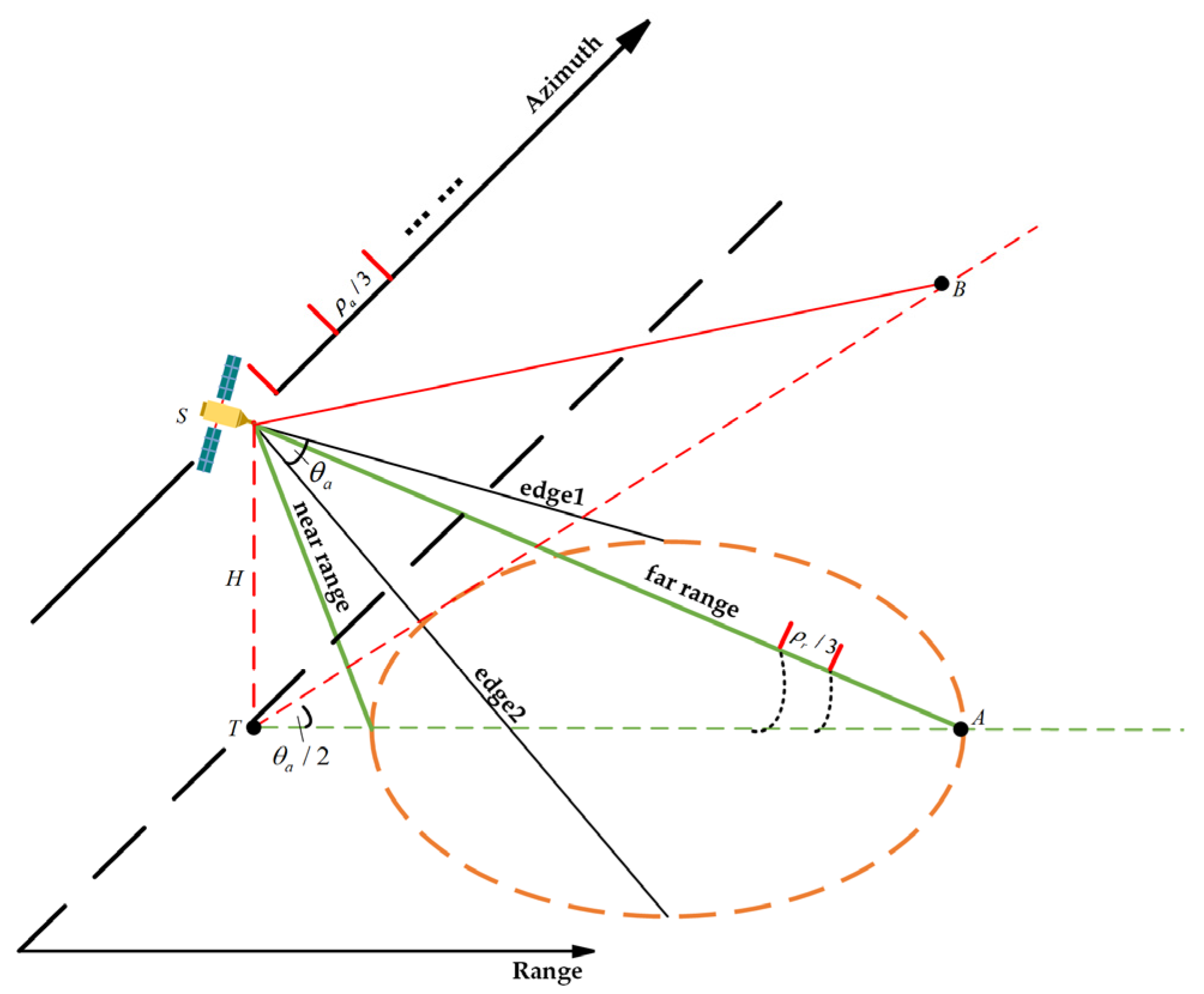
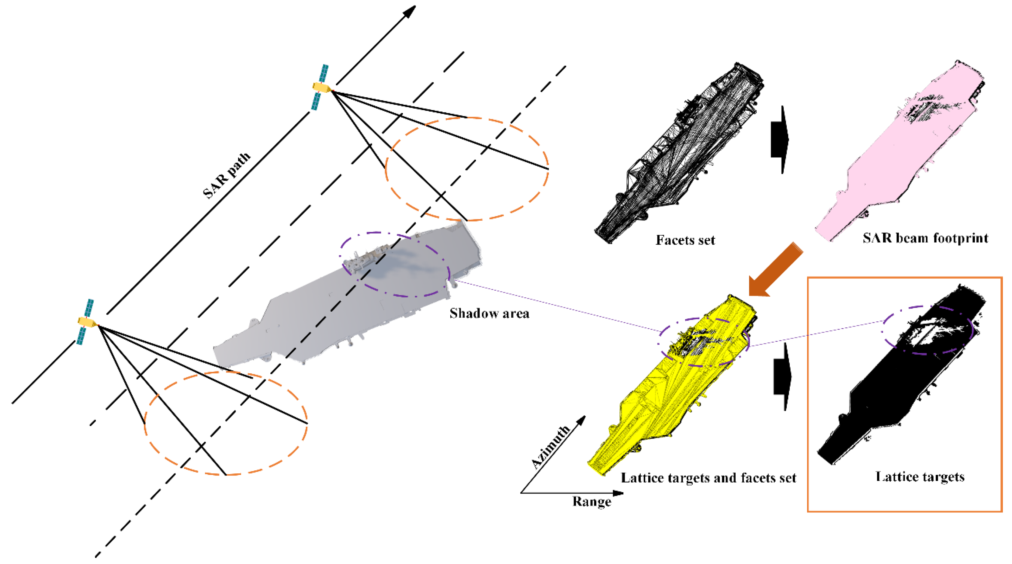
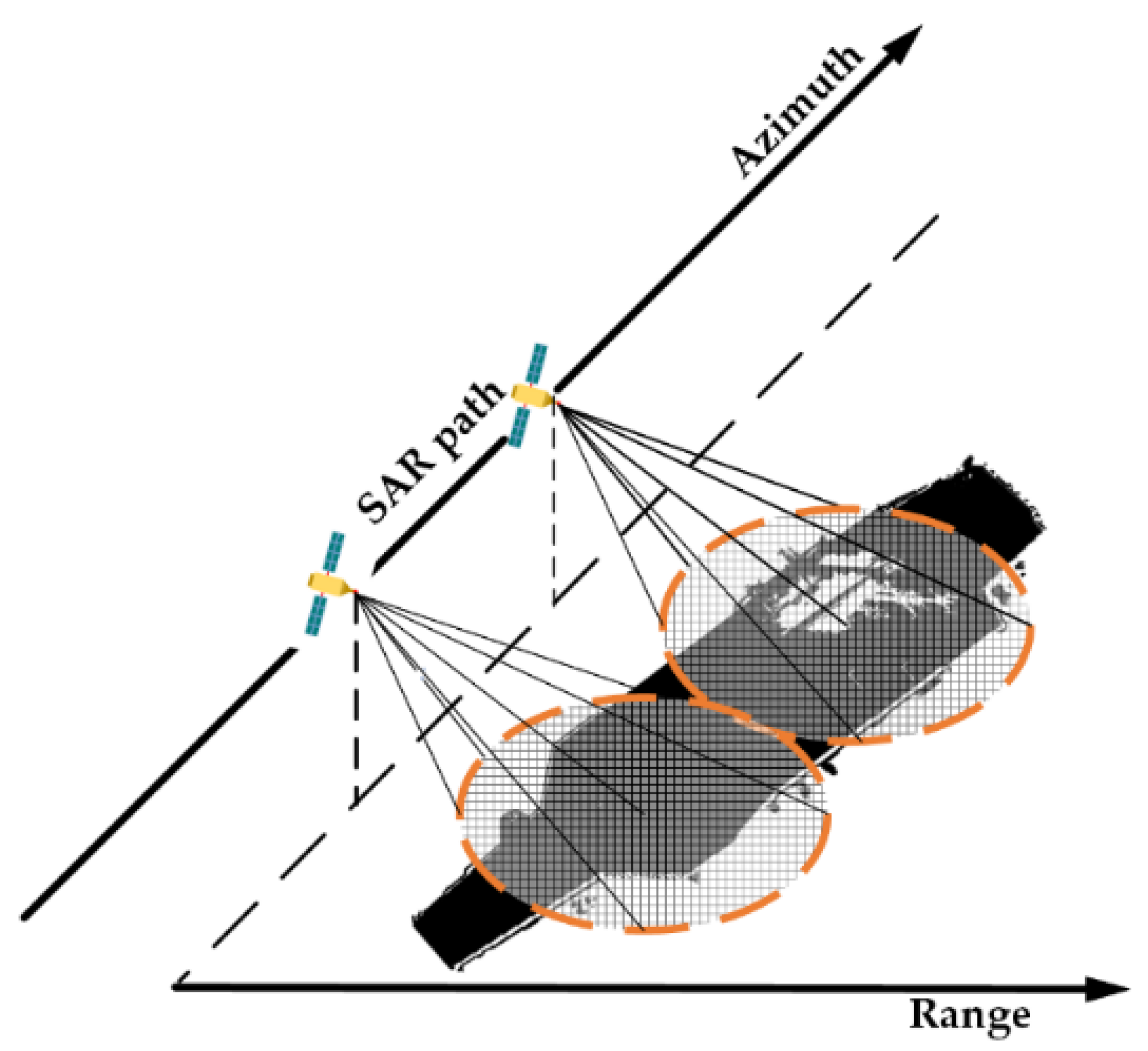
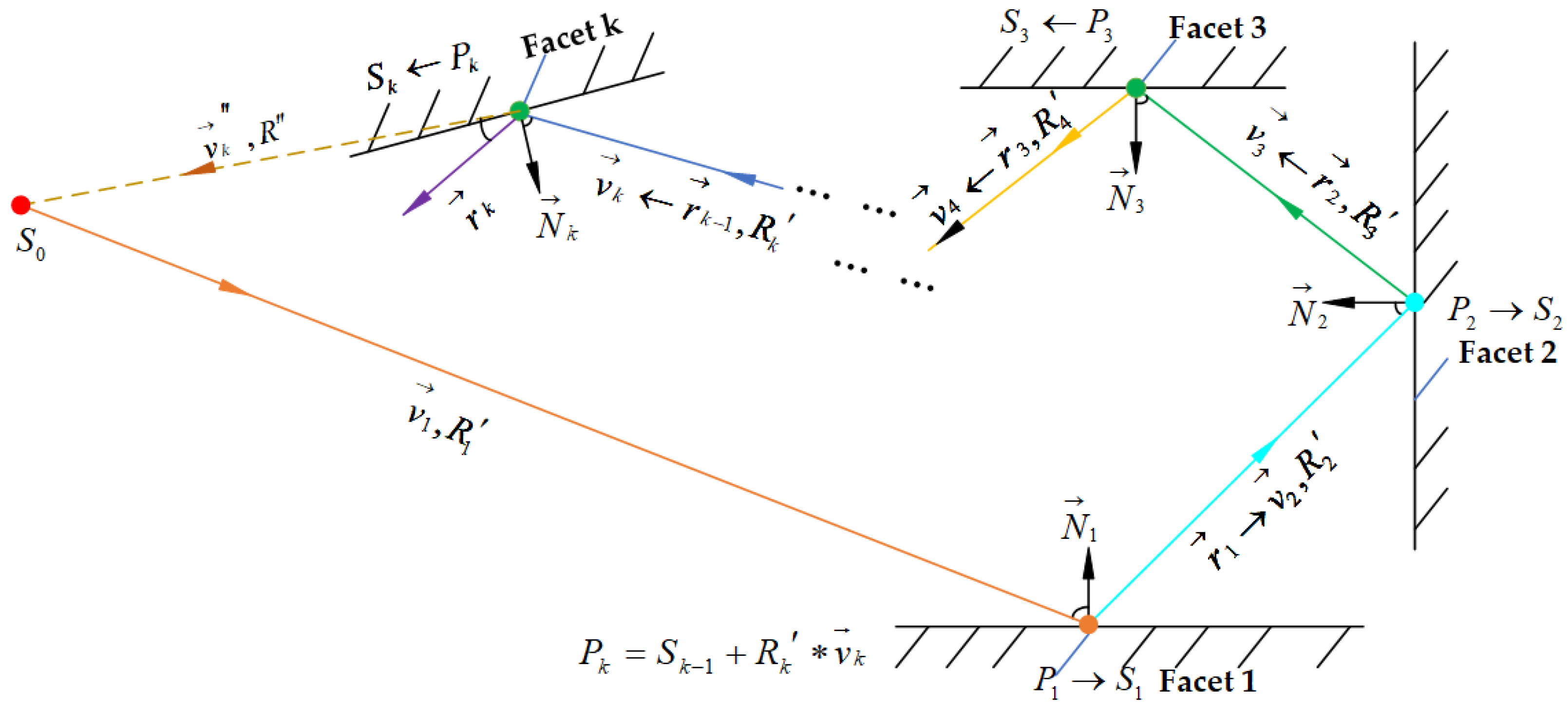
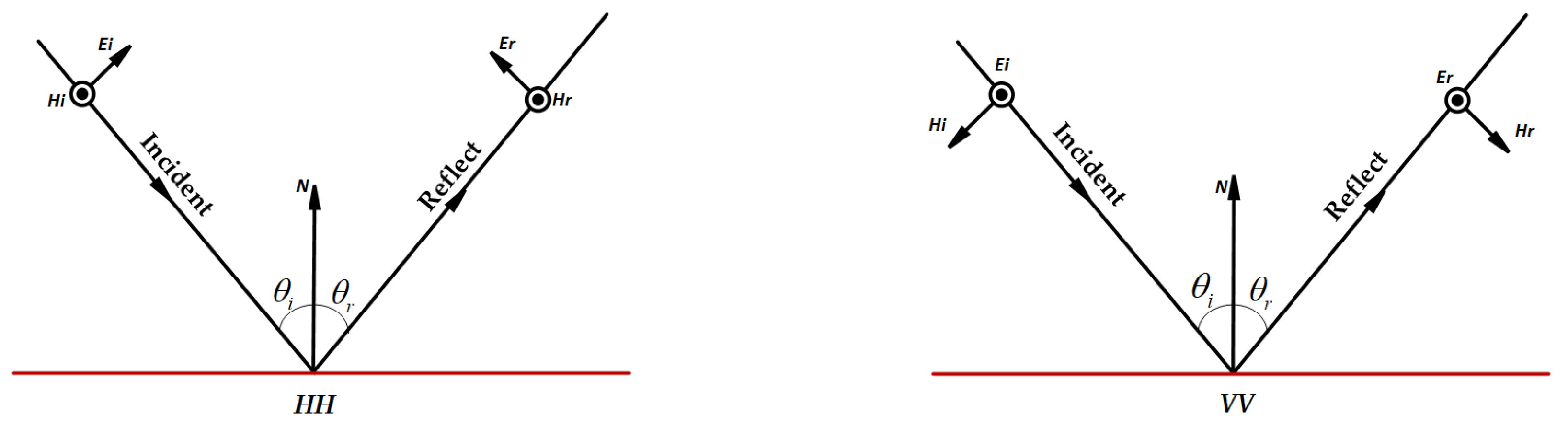
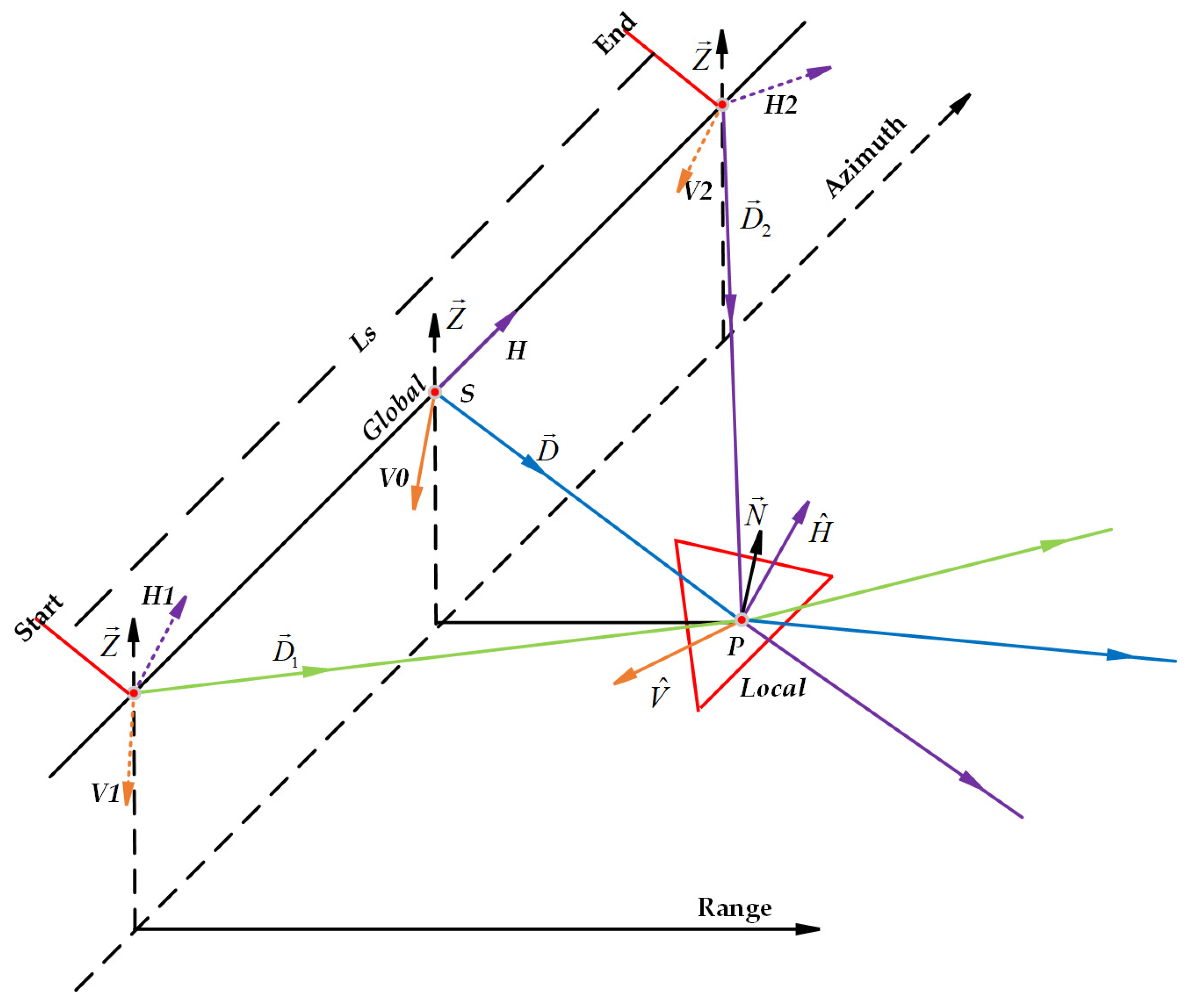
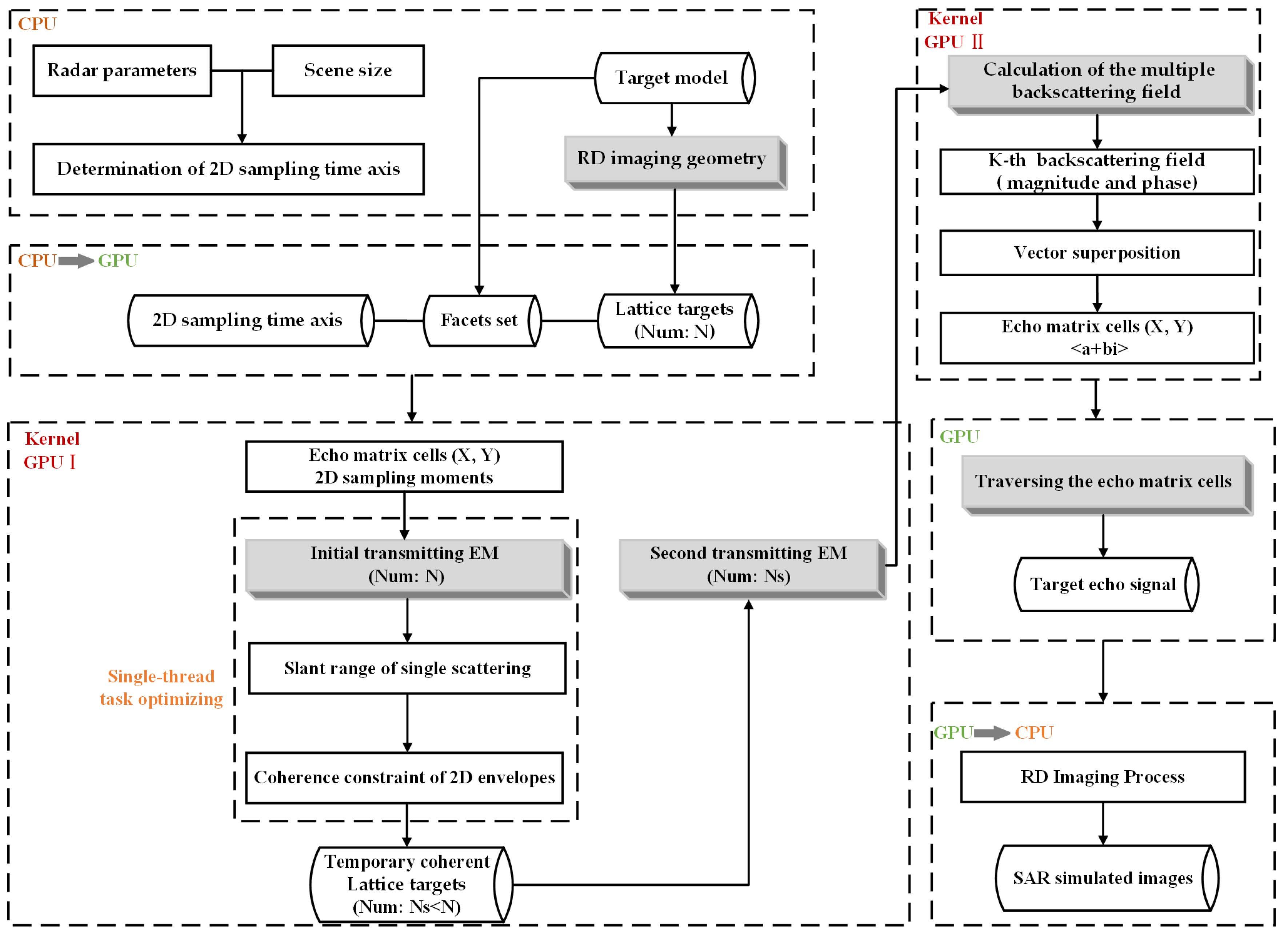
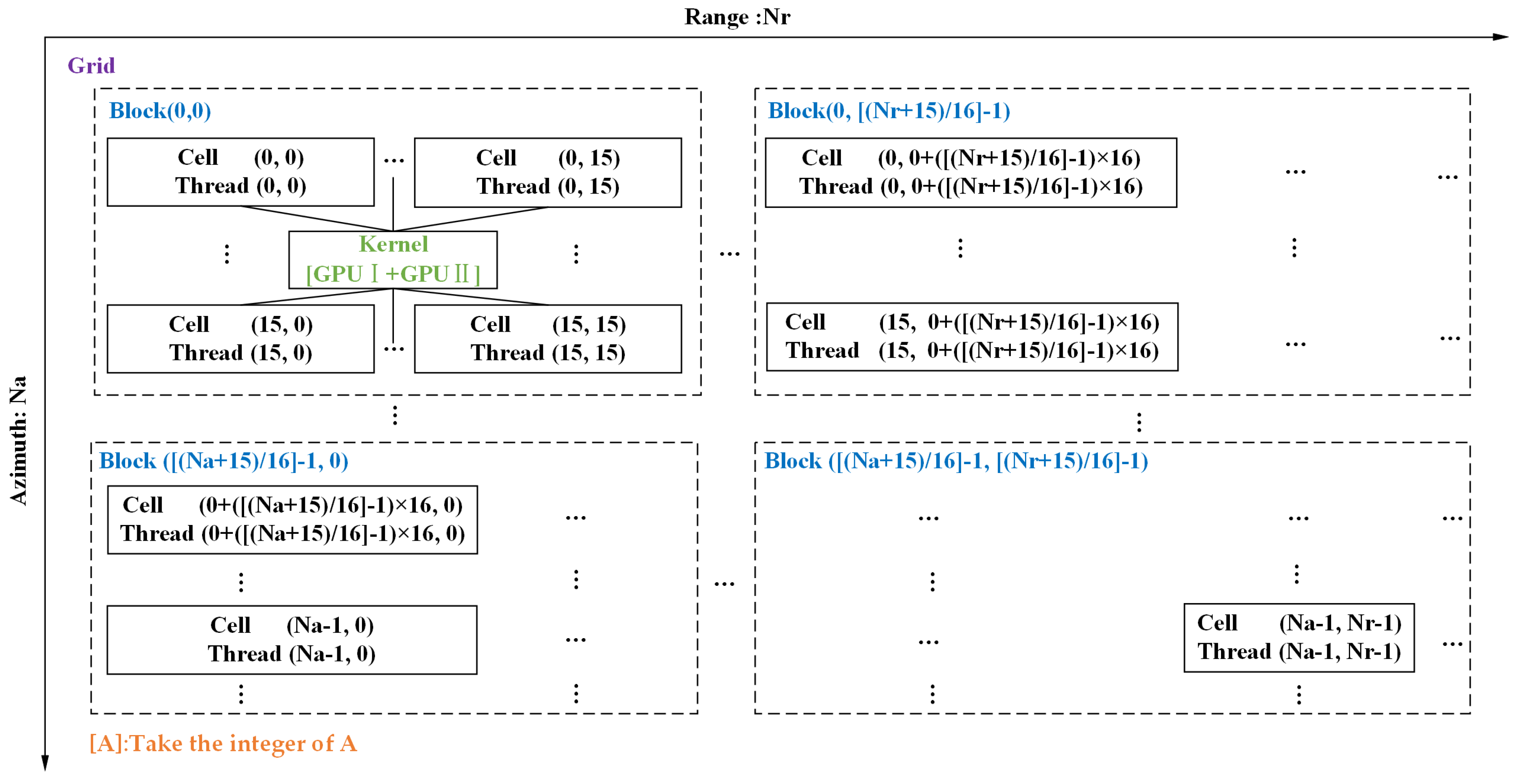
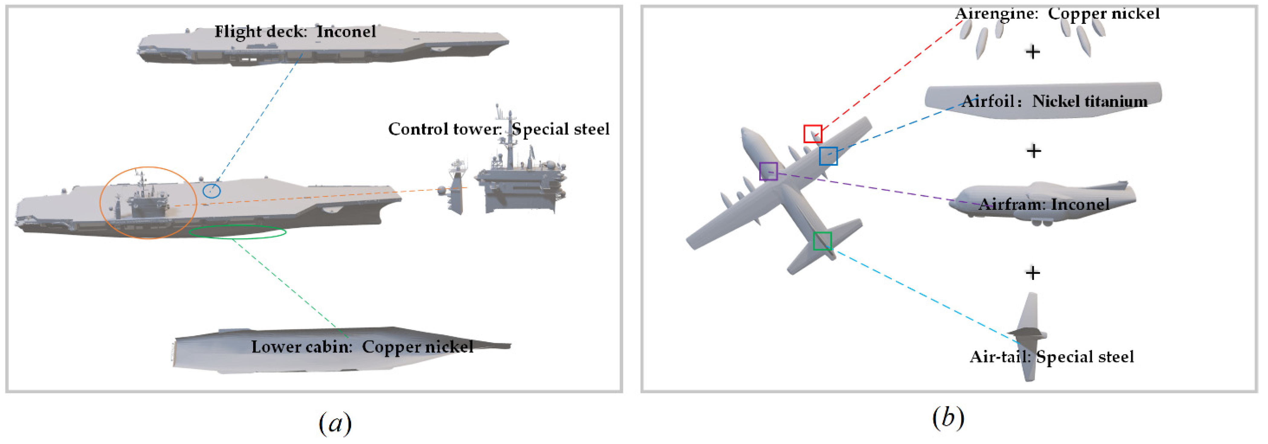
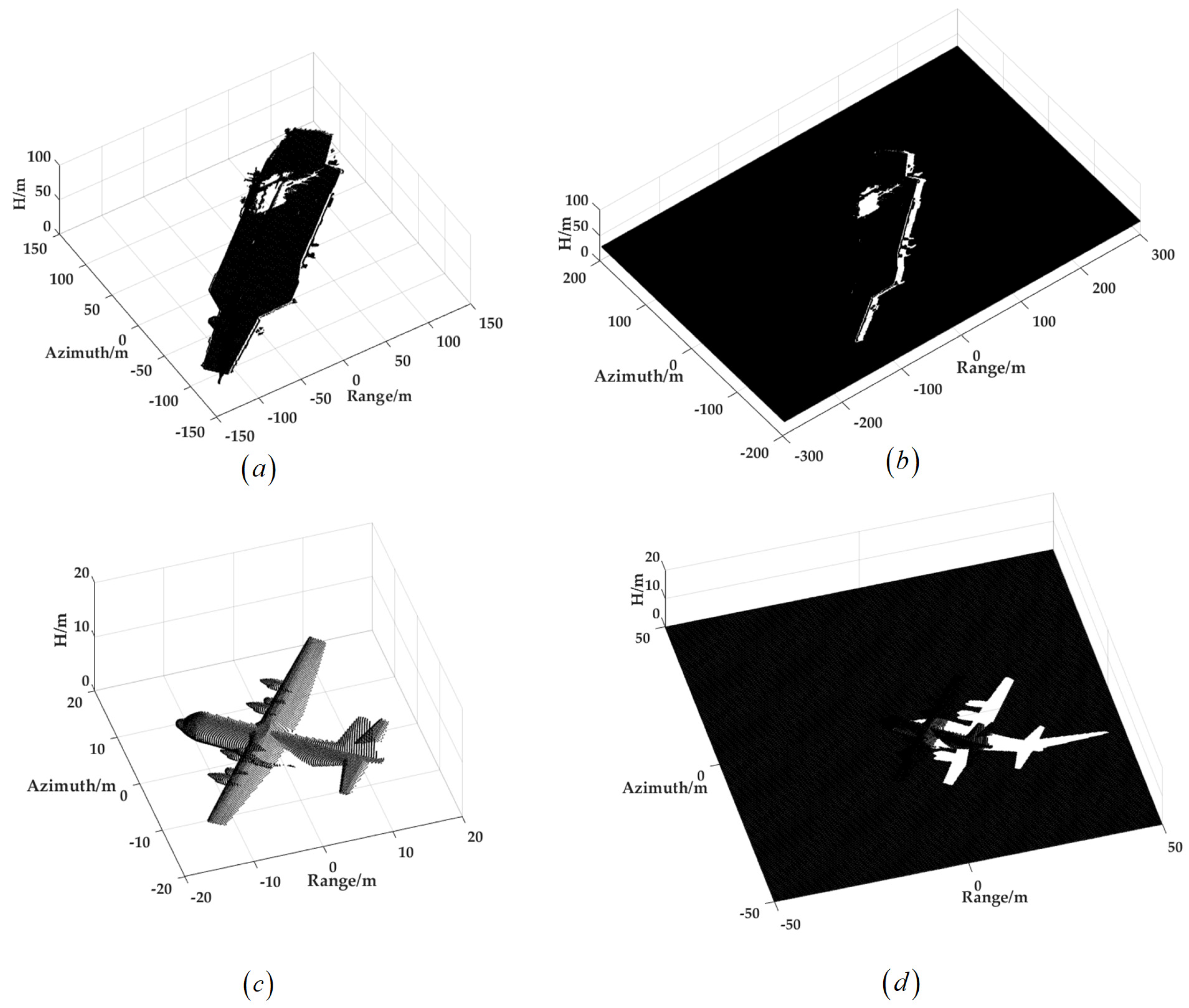
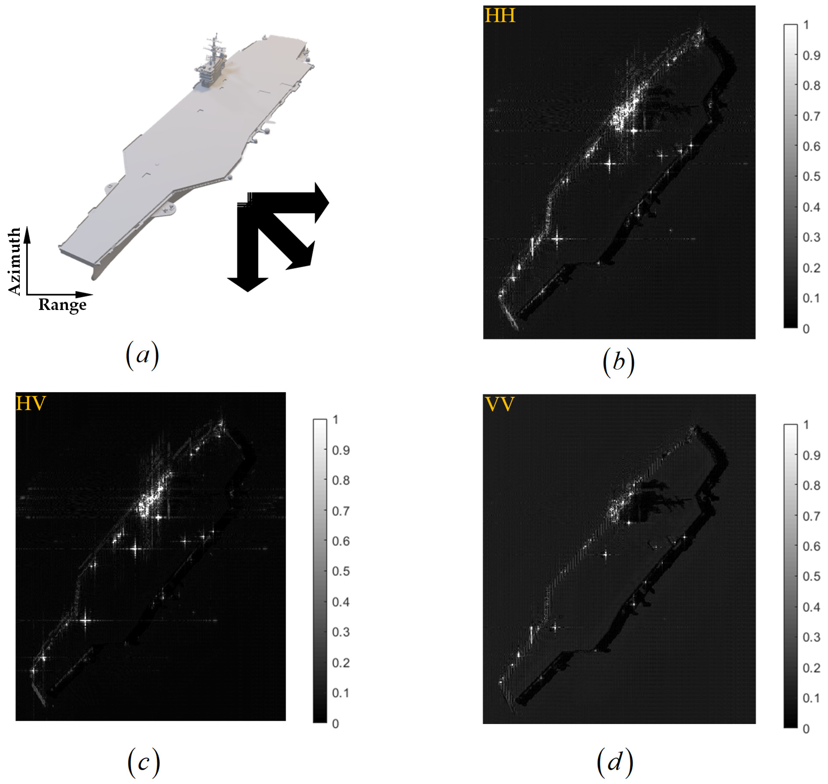
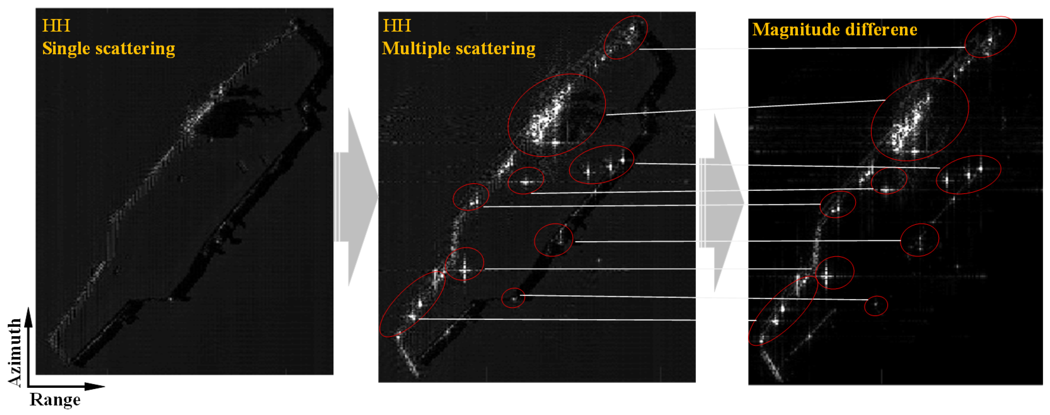
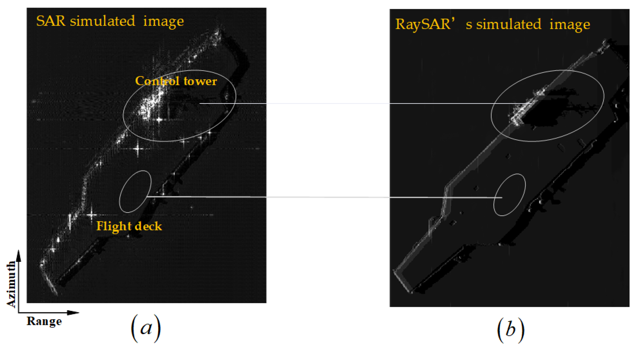
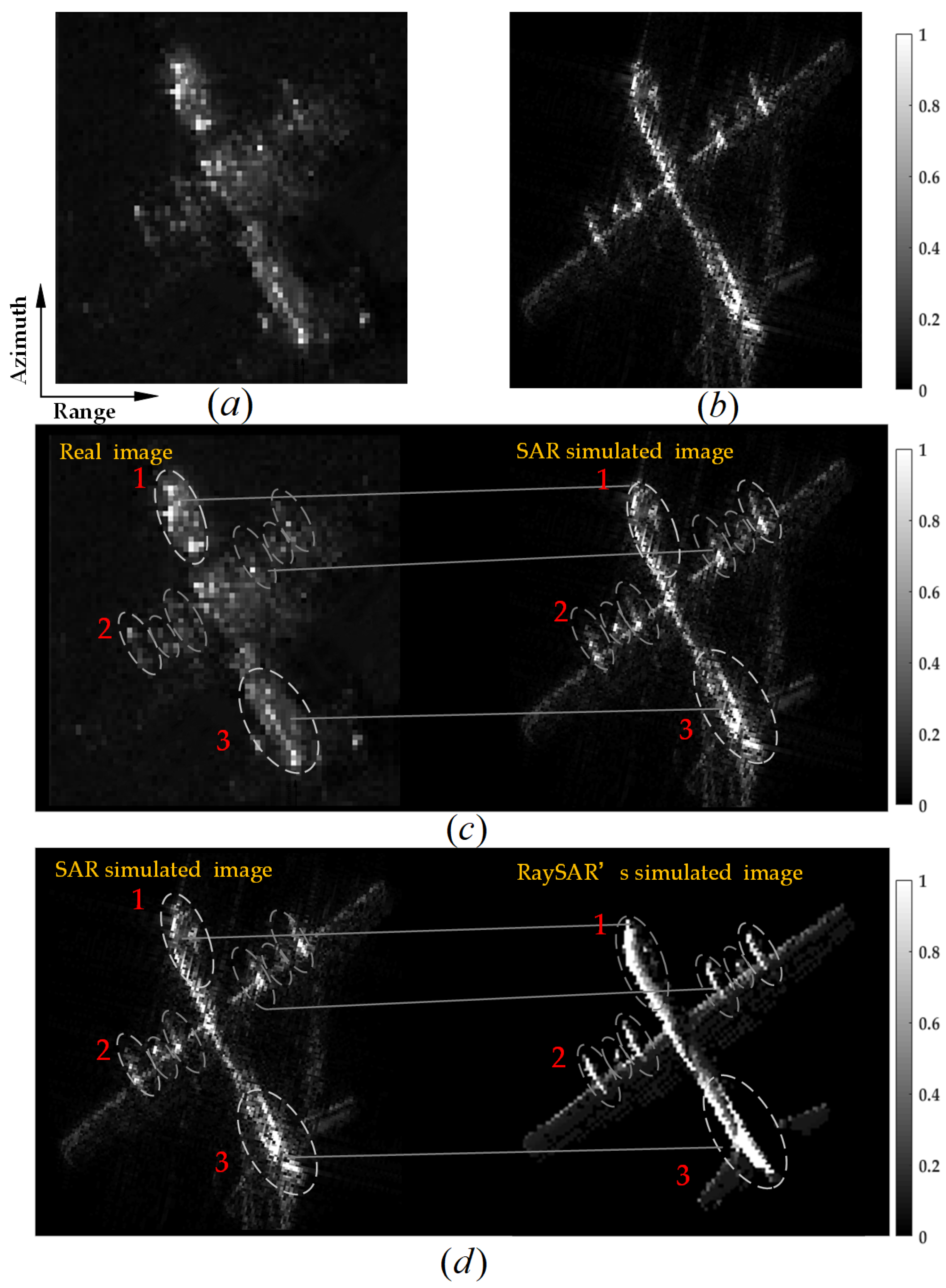
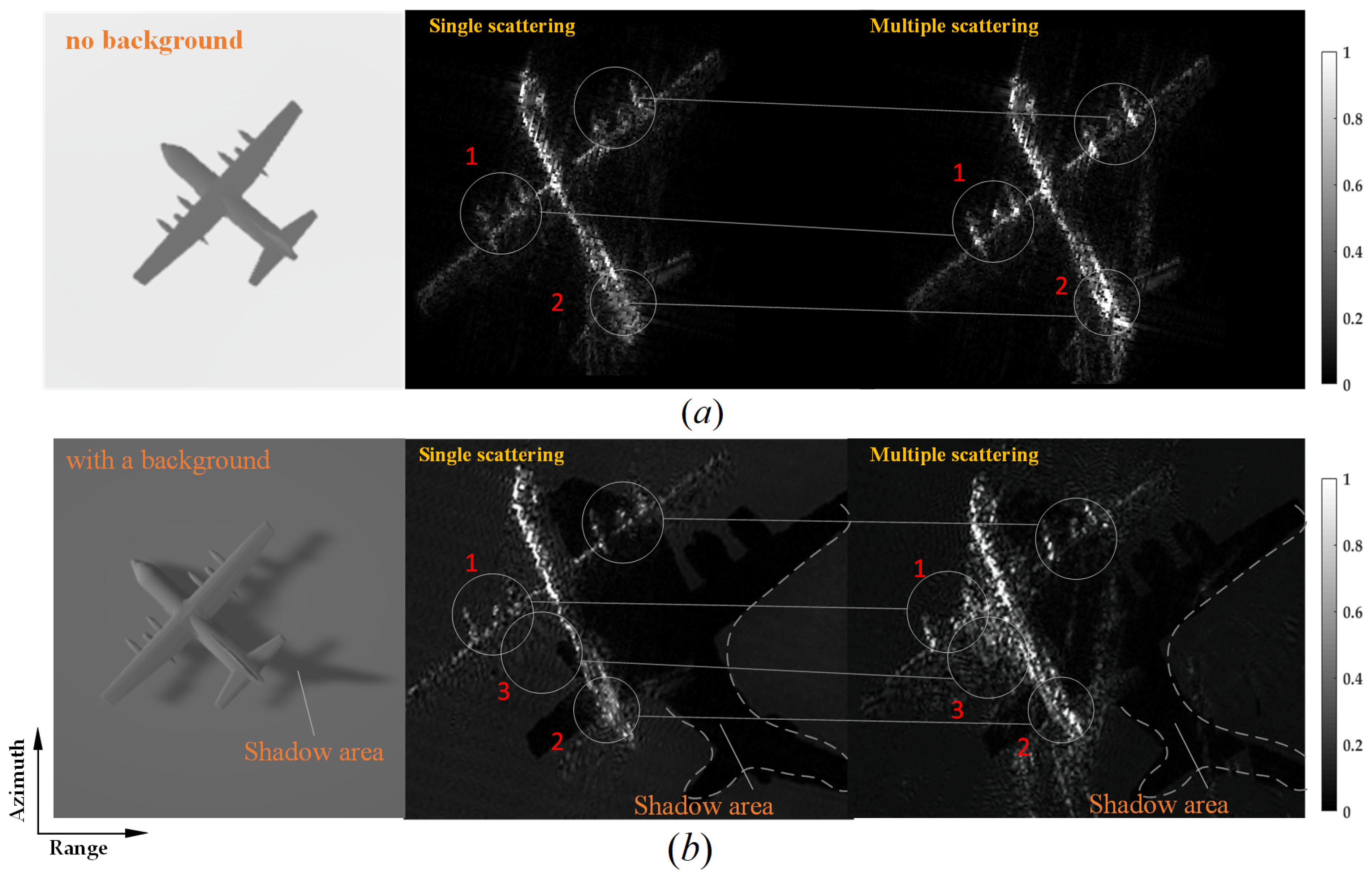
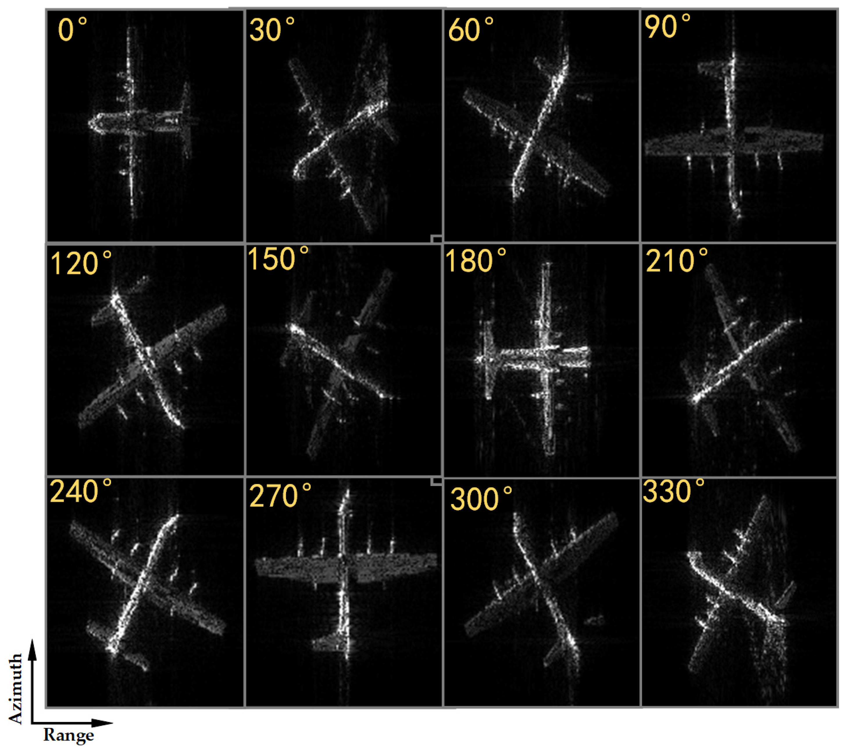
Table 1.
SAR system parameters.
| Parameter | Value |
|---|---|
| Model | Aircraft carrier and airplane |
| Signal form | Linear FM signal |
| Bandwidth | 180 MHz |
| Pulse duration | 1.0 μs |
| Range resolution | 1.0 m |
| Incidence angle | 60°/59.92° |
| Center frequency | 15 GHz |
| Platform height | 2 km |
| Effective radar velocity | 300 m/s |
| Doppler bandwidth | 400 Hz |
| PRF | 450 Hz |
| Slant range of scene center | 4 km |
| Azimuth resolution | 1.0 m |
| Squint angle | 0° |
Table 2.
Material property parameters.
| Material (Main Component) | Relative Permittivity | Diffuse Coefficient | Specular Coefficient | Specular Index | Energy Decay Coefficient |
|---|---|---|---|---|---|
| Aluminum | 8.00 | 0.75 | 0.80 | 50.00 | 0.20 |
| Fiber reinforced plastics | 8.50 | 0.80 | 0.60 | 50.00 | 0.10 |
| Special steel | 9.50 | 0.65 | 0.80 | 30.00 | 0.25 |
| Copper nickel | 12.00 | 0.70 | 0.50 | 50.00 | 0.15 |
| Inconel | 10.50 | 0.75 | 0.40 | 30.00 | 0.10 |
| Nickel titanium | 15.00 | 0.65 | 0.70 | 40.00 | 0.20 |
Table 3.
Computing environment.
| GPU | CUDA Version | Graphics Memory | Compiler Environment | CPU | Total Memory Size | Operation System |
|---|---|---|---|---|---|---|
| NVIDIA GeForce RTX3060 | 10.0 | 6G | VS2019 | 11th Gen Intel(R) Core (TM) i7-11800H | 16G | Windows10 |
Table 4.
Simulation time consumption comparison of aircraft carrier with a background.
| Model | SAR Image Size | Aspect Angle | Lattices Number | CPU Time | GPU Time | Speedup Rate | |
|---|---|---|---|---|---|---|---|
| Aircraft Carrier | Azimuth | 654 samples | 60° | 2,139,736 | 181.89 h | 0.98 h | 185.6× |
| Range | 960 samples | ||||||
Table 5.
The similarity metrics between the simulated airplane image and the real SAR image (No 1) as well as the RaySAR-simulated image (No 2), respectively.
Table 5.
The similarity metrics between the simulated airplane image and the real SAR image (No 1) as well as the RaySAR-simulated image (No 2), respectively.
| Reference Image No. | Normalized Cross-Correlation | Cosine Similarity | Mean Hash Similarity |
|---|---|---|---|
| 1 | 0.85 | 0.92 | 0.86 |
| 2 | 0.90 | 0.96 | 0.93 |
Table 6.
Simulation time consumption comparison of airplane without a background.
| Model | SAR Image Size (HH) | Aspect Angle | Lattices Number | CPU Time | GPU Time | Speedup Rate | |
|---|---|---|---|---|---|---|---|
| Airplane | Azimuth | 378 samples | 0° | 8756 | 52.60 h | 0.31 h | 169.7× |
| 60° | 9148 | 47.35 h | 0.27 h | 175.4× | |||
| 120° | 11,929 | 35.97 h | 0.23 h | 156.5× | |||
| Range | 667 samples | ||||||
| 180° | 7923 | 49.26 h | 0.33 h | 149.3× | |||
| 240° | 11,834 | 48.05 h | 0.29 h | 165.7× | |||
| 300° | 12,191 | 52.05 h | 0.30 h | 173.5× | |||
Disclaimer/Publisher’s Note: The statements, opinions and data contained in all publications are solely those of the individual author(s) and contributor(s) and not of MDPI and/or the editor(s). MDPI and/or the editor(s) disclaim responsibility for any injury to people or property resulting from any ideas, methods, instructions or products referred to in the content. |
© 2023 by the authors. Licensee MDPI, Basel, Switzerland. This article is an open access article distributed under the terms and conditions of the Creative Commons Attribution (CC BY) license (https://creativecommons.org/licenses/by/4.0/).
Share and Cite
MDPI and ACS Style
Wu, K.; Jin, G.; Xiong, X.; Zhang, H.; Wang, L. Fast SAR Image Simulation Based on Echo Matrix Cell Algorithm Including Multiple Scattering. Remote Sens. 2023, 15, 3637. https://doi.org/10.3390/rs15143637
AMA Style
Wu K, Jin G, Xiong X, Zhang H, Wang L. Fast SAR Image Simulation Based on Echo Matrix Cell Algorithm Including Multiple Scattering. Remote Sensing. 2023; 15(14):3637. https://doi.org/10.3390/rs15143637
Chicago/Turabian StyleWu, Ke, Guowang Jin, Xin Xiong, Hongmin Zhang, and Limei Wang. 2023. "Fast SAR Image Simulation Based on Echo Matrix Cell Algorithm Including Multiple Scattering" Remote Sensing 15, no. 14: 3637. https://doi.org/10.3390/rs15143637
Note that from the first issue of 2016, this journal uses article numbers instead of page numbers. See further details here.