
Refraction Correction for Spectrally Derived Bathymetry Using UAS Imagery


Geomatics Group, School of Civil and Construction Engineering, Oregon State University, Corvallis, OR 97331, USA
*
Author to whom correspondence should be addressed.
Remote Sens. 2023, 15(14), 3635; https://doi.org/10.3390/rs15143635
Submission received: 30 May 2023
/
Revised: 16 July 2023
/
Accepted: 19 July 2023
/
Published: 21 July 2023
Abstract
:Spectrally derived bathymetry (SDB) algorithms are rapidly gaining in acceptance and widespread use for nearshore bathymetric mapping. In the past, refraction correction could generally be ignored in SDB, due to the relatively small fields of view (FOVs) of satellite sensors, and the fact that such corrections were typically small in relation to the uncertainties in the output bathymetry. However, the validity of ignoring refraction correction in SDB is now called into question, due to the ever-improving accuracies of SDB, the desire to use the data in nautical charting workflows, and the application of SDB algorithms to airborne cameras with wide FOVs. This study tests the hypothesis that refraction correction leads to a statistically significant improvement in the accuracy of SDB using uncrewed aircraft system (UAS) imagery. A straightforward procedure for SDB refraction correction, implemented as a modification to the well-known Stumpf algorithm, is presented and applied to imagery collected from a commercially available UAS in two study sites in the Florida Keys, U.S.A. The results show that the refraction correction produces a statistically significant improvement in accuracy, with a reduction in bias of 46–75%, a reduction in RMSE of 3–11 cm, and error distributions closer to Gaussian.
1. Introduction
Photogrammetric and optical remote sensing methods have long been of interest for mapping bathymetry in nearshore coastal areas [1,2,3,4,5]. Although these methods typically do not meet the same accuracies as boat-based sonar, they can be invaluable for filling in nearshore data voids in areas that are remote, inaccessible, and/or dangerous. Additionally, optical remote sensing methods of bathymetry retrieval can be highly efficient and cost-effective. Important uses of these methods include mapping of coral reefs and other ecologically important benthic habitats [6,7,8], seafloor morphologic change analysis [9,10], and support of hydrographic surveying [11,12,13], among others.
The primary active remote sensing technology for bathymetric mapping is bathymetric lidar [14]. Meanwhile, methods based on passive, optical imaging fall into three categories, which can trace their origins back to the 1940s [1,5]. The first category, often referred to as “photobathymetry” in early studies, is based on stereophotogrammetry and has seen a recent surge in interest using—structure from motion (SfM) photogrammetry, e.g., [15]. We refer to these methods as stereobathymetry. The second main category of approach, which we mention for completeness but is outside the scope of this study, is based on surface wave kinematics (i.e., the decrease in celerity and wavelength and increase in amplitude with decreasing depth in areas in which waves can “sense” the seafloor), using multiple images collected at precisely known time intervals [16,17]. The third main type of approach, spectrally derived bathymetry (SDB), retrieves bathymetry from spectral image bands, based on the spectral attenuation of light with depth [3,18,19,20,21,22] and references therein. It should be noted that most authors who use the term SDB define it as an acronym for satellite-derived bathymetry. However, following the convention of [23], we take the “S” in SDB to refer to “spectral”, rather than “satellite”, as it is more descriptive of the approach, rather than the type of platform used to acquire the data. In fact, SDB algorithms can equally well be applied to airborne imagery, including imagery from uncrewed aircraft systems (UAS), as in this study. Within SDB, there are various broad categories of approaches, some more analytical and others more empirical, but all are based on the spectral attenuation of irradiance with depth, which can be modeled using the Beer–Lambert Law.
Both bathymetric lidar and stereobathymetry, which can be formulated mathematically as ray-tracing procedures, require refraction correction to account for the change in the direction and corresponding change in the speed of light at the air–water interface, e.g., [24,25,26]. Refraction correction moves the elevations of (uncorrected) bathymetric points up in bathymetric lidar and down in stereobathymetry. This is because lidar is based on time-of-flight calculations, which are a function of speed of light, which decreases when light enters the water column. In contrast, stereobathymetry is based on the geometric intersection of rays from overlapping images, with the point of intersection being too shallow, if refraction is ignored. Neglecting refraction correction would lead to errors of ~25% of the uncorrected depth in bathymetric lidar [25] and ~33% of the uncorrected depth in stereophotogrammetry, depending on the image locations of a specific bathymetric point in the overlapping images, and the base–height ratio [2,3,4,5,6,7,8,9,10,11,12,13,14,15].
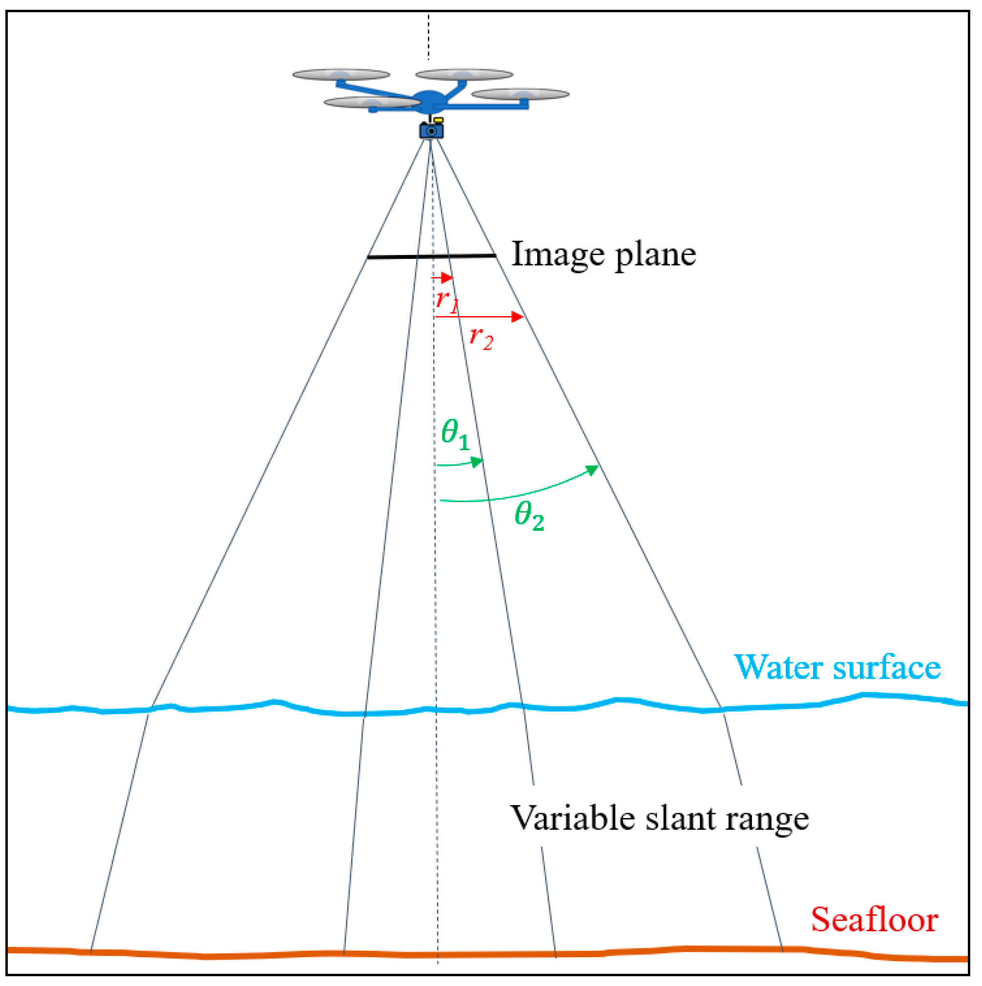
In contrast to bathymetric lidar and stereobathymetry, refraction correction in SDB has received relatively little attention, although a small number of studies, e.g., [23,27], have explicitly considered the variable slant range of light rays through the water column. As a note on terminology, what we refer to as SDB refraction correction could equally well be termed “slant–range correction” or “off-nadir geometric correction” or “radial geometric correction”. Specifically, we define SDB refraction correction as the correction for the variable slant range of light reflected from the seafloor to the imaging sensor within the imaging sensor’s field of view (Figure 1).
The SDB refraction correction is a function of incidence angle, the refractive index of the water, and depth. It is likely that the main reasons this correction has received relatively little attention in the published literature to date are that (a) with small FOV sensors, such as the Operational Land Imager (OLI) onboard Landsat 8 and 9 and the Multispectral Instrument (MSI) on Sentinel-2A and -2B, the refraction correction is relatively small (Figure 2 and Table 1), and (b) SDB uncertainties have generally been large enough that refraction correction could reasonably be neglected. However, both of these facts are currently called into question. First, with SDB algorithms currently being applied to imagery acquired from airborne platforms, both planes and UAS [28], the assumption of a small FOV is no longer valid. Second, accuracies of SDB are improving due to new algorithms and procedures, and the desire to be able to use SDB for nautical charting purposes, e.g., [11,13,29].
Based on the above considerations, the goals of this study are to (1) test the hypothesis that refraction correction leads to a statistically significant improvement in SDB accuracy when applied to images from a commercially available and widely used UAS and (2) develop and test a model that is straightforward to implement, using only readily available parameters as input.
2. Methods
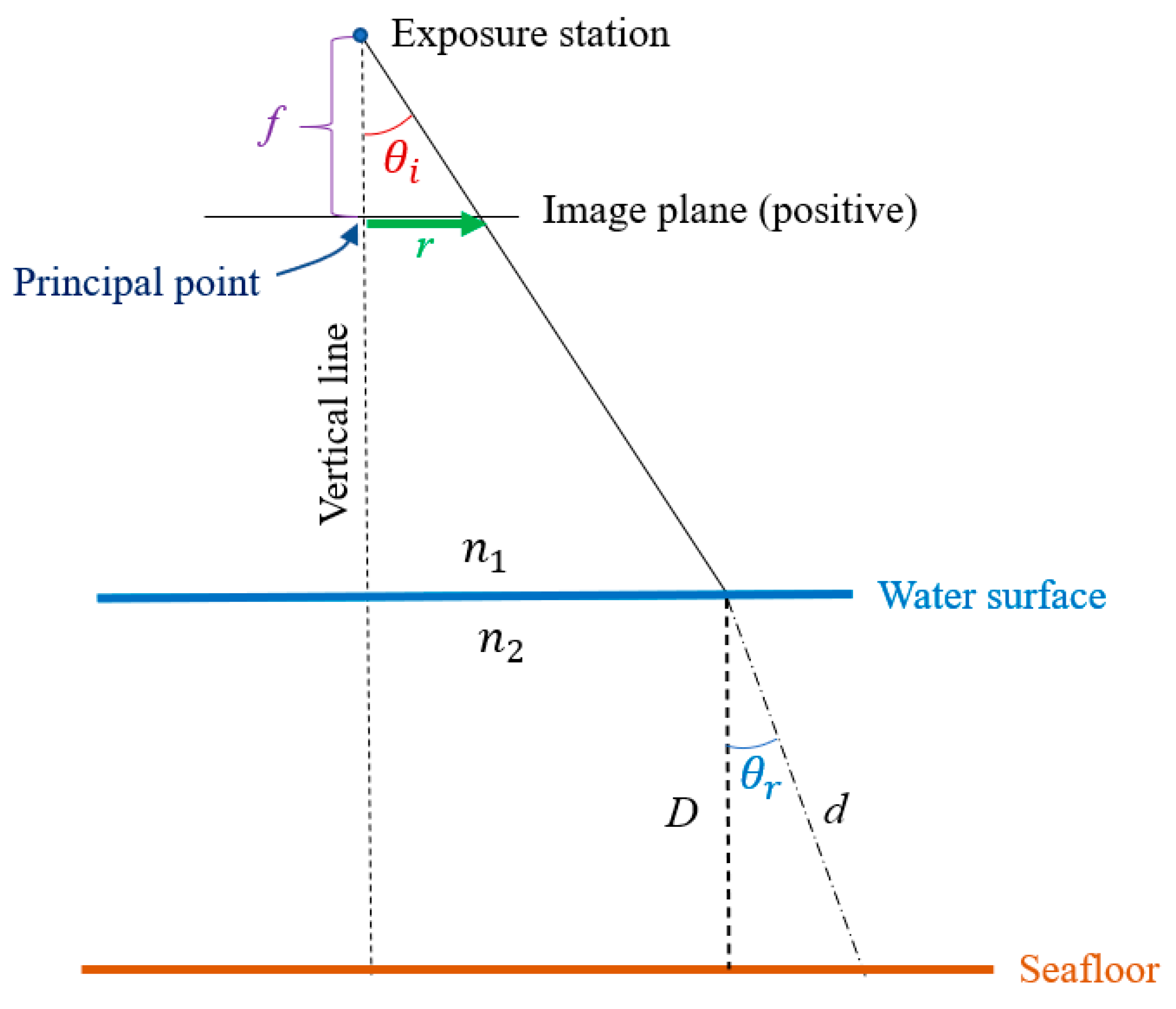
SDB algorithms predict the water depth of a pixel based on relative changes in band values (or logarithms of band values) with depth, due to spectral attenuation with path length through the water column. Off-nadir, the path through the water column traversed by a ray of light from the seafloor to the camera lens is greater than the actual depth. The geometry is illustrated graphically in Figure 3. Here, f is the focal length, r is image radial distance (i.e., the distance in image space from the principal point to the image point in question), is the incidence angle, is the angle of refraction at the air–water interface, n1 is the refractive index of air, n2 is the refractive index of water, d is the uncorrected depth (slant range of light ray reflected diffusely by the seafloor, traveling through the water column, refracted at the air-water interface, and incident on the camera lens), and D is the corrected depth.
In order to derive an easy-to-implement refraction correction procedure, we start with the simplifying assumption that the image is vertical, meaning the optical axis is aligned with a vertical line (plumb line), as depicted in Figure 3. This is a reasonable assumption for aerial imagery which is intended to be vertical, since, in this case, image tilt is typically <1° and almost always <3° [30]. However, the impacts of this assumption will be addressed later. The second simplification underlying our refraction correction procedure is that we consider only the one-way travel path of a light ray from the seafloor to the camera lens, rather than the entire path from the sun to the seafloor to the camera lens. In turn, this assumes a uniformly illuminated seafloor and Lambertian reflection of visible light from the seafloor. Starting with these assumptions and the geometry depicted in Figure 3, we derive a refraction correction (specifically, a correction to d), as a function of radial image distance, r. Using Snell’s law,
we define the refraction correction, , as the ratio of the corrected to uncorrected depth, and calculate it as follows:
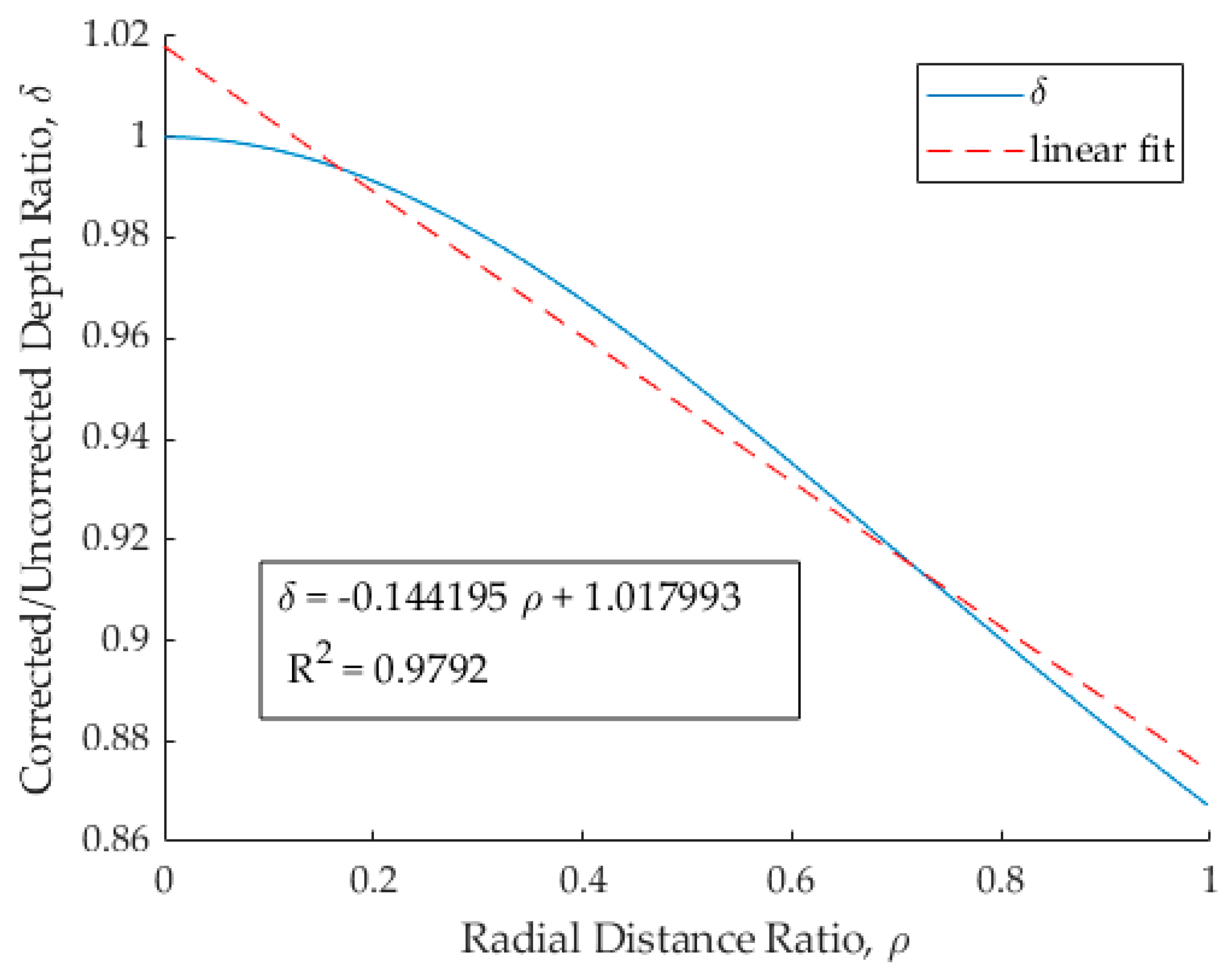
Importantly, the refraction correction of Equation (2) can be expressed as a function of radial image distance, which is a straightforward parameter to compute, making use of the fact that . We measure the radial distance from the principal point, which we take to be the center of the image sensor. For the purposes of this study, it is entirely reasonable to assume that principal point offsets can be safely ignored, as they are generally <1 pixel. Rather than using an absolute radial distance (with physical units, such as millimeters), we define a radial distance ratio, , as the radial distance of each pixel divided by the maximum radial distance (i.e., the distance from the center to the camera chip to the corners). The relationship between and is plotted graphically in Figure 4 for one particular camera and an assumed seawater refractive index of 1.3422 (wavelength = 500 nm, temperature = 28 °C, and salinity = 35‰).
The vs. curve shown in Figure 4 can be fit with a cubic polynomial with an R2 of 1.00. However, we seek a parsimonious model that will tend to avoid overfitting and requires only a small number of parameters for which we will need to solve. We note that a linear function can also represent this relationship sufficiently, with an R2 of 0.979. The form of the linear relationship is:
where α and β are constants. Equation (3) could be used to compute the refraction corrected depth directly, i.e.,
The coefficients (α, β) in Equation (4) are a function of the refractive index of the water in the scene (which, in turn, depends on wavelength, temperature, and salinity) and the parameters of the camera (FOV, focal length, and physical chip size). Because these parameters may not be precisely known in practice, rather than solving for them analytically, we use a data-driven approach in which the parameters are automatically computed as part of the refraction-corrected SDB procedure. Our refraction-corrected SDB model is an extension of the well-known Stumpf SDB algorithm, in which SDB is computed as [19,20]:
where d is depth and pSDB is relative bathymetry, computed as , where Rb and Rg are the blue and green band reflectances, n is a constant chosen to ensure positive logarithms and linear response (set to 1000 in our work, following, e.g., [31]), and m0 and m1 are coefficients of a linear transformation obtained by regressing reference depths on pSDB. The reference depths can be from an existing nautical chart, ICESat-2 bathymetry [25,31], or any other existing source of bathymetry. The Stumpf algorithm is widely used [31,32,33,34,35,36], and, importantly for our research group, it is used in the National Oceanic and Atmospheric Administration (NOAA) SatBathy software tool [37,38]. Based on the form of Equation (4), we present a modified version of the Stumpf equation, which incorporates refraction correction via the radial distance ratio, ρ, as follows:
It should be noted that, in comparison to the original Stumpf algorithm (Equation (5)), our refraction corrected version (Equation (6)) has four parameters (m0, m1, m2, and m3), rather than the original two. However, if there are at least four reference soundings, it is possible to solve for the unique values of the four parameters, and, if there are more than four reference soundings, a least squares solution is possible.
To achieve the highest accuracy, applying radial lens distortion corrections before the refraction correction is important, since (a) the refraction correction is computed as a function of radial distance and (b) the non-metric cameras used on UAS tend to have large amounts of lens distortion, compared to the large-format, film-based metric mapping aerial cameras of past decades. Symmetric radial lens distortion can be modeled mathematically in multiple ways, but often as a polynomial in radial distance, r, with the coefficients {ki} determined through an appropriate lens calibration procedure [30].
3. Experiment
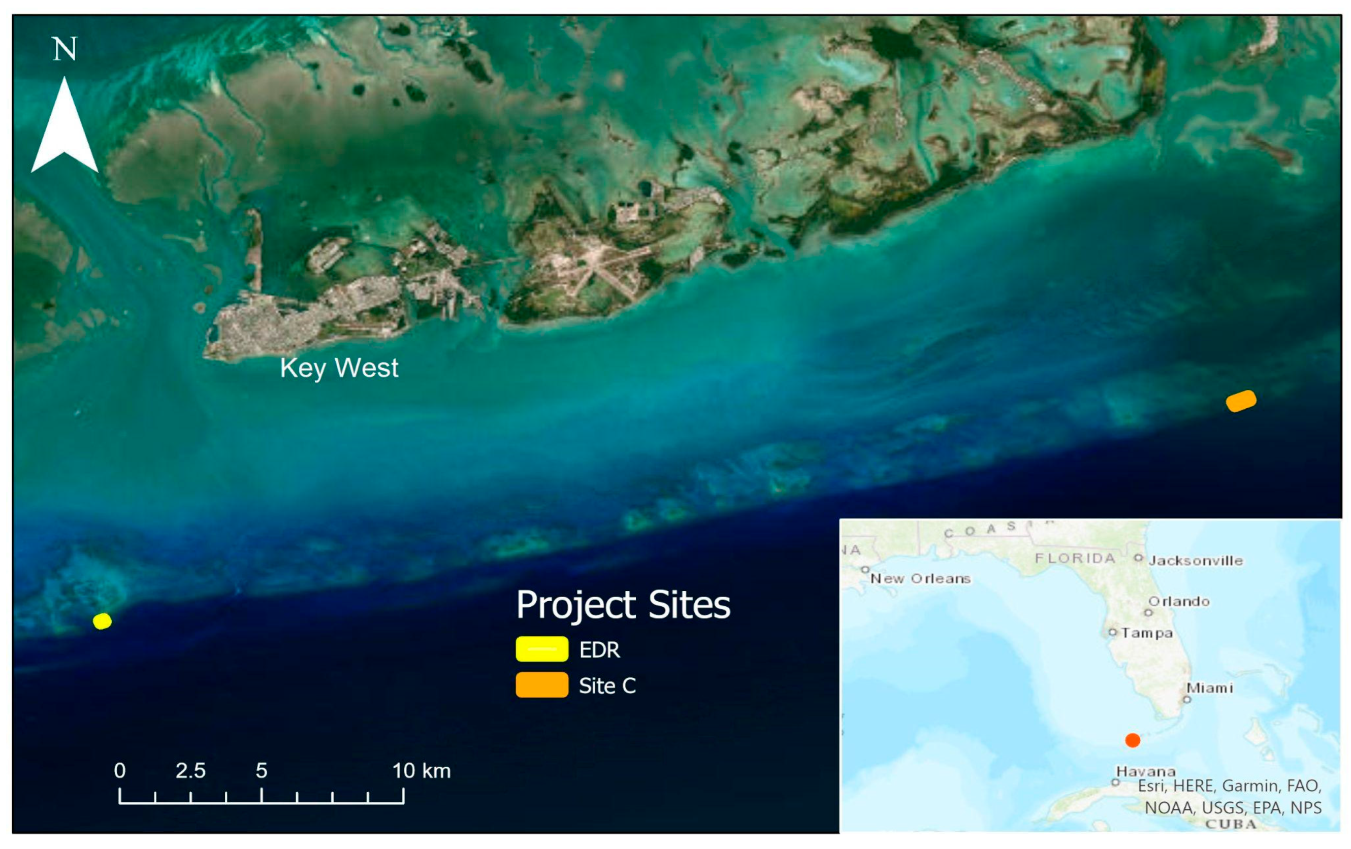
The data for this study were collected from 19–25 June 2022, at two sites in the Florida Keys, referred to as Eastern Dry Rocks (EDR) and Site C. Both are coral restoration sites managed by the Mote Marine Laboratory, and the collection was performed as part of a broader project investigating the ability to map and monitor coral reef change over time, a collaborative effort of the NOAA, the University of New Hampshire (UNH) Center for Coastal and Ocean Mapping (CCOM) Joint Hydrographic Center (JHC), the Mote Marine Laboratory, and Oregon State University. We selected two sites to be representative of different bottom types found in the Florida Reef Tract. EDR contains a spur-and-groove reef structure extending from the shallow backreef out to depths of ~4–6 m. Further offshore is a forereef terrace with a combination of hardbottom and remnant spur-and-groove providing high relief. In contrast, Site C is a high-relief ledge comprised with high vegetation diversity, concentrated within 5–10 m of the sand/reef margin, transitioning rapidly to barren hardbottom with considerably lower complexity [39].
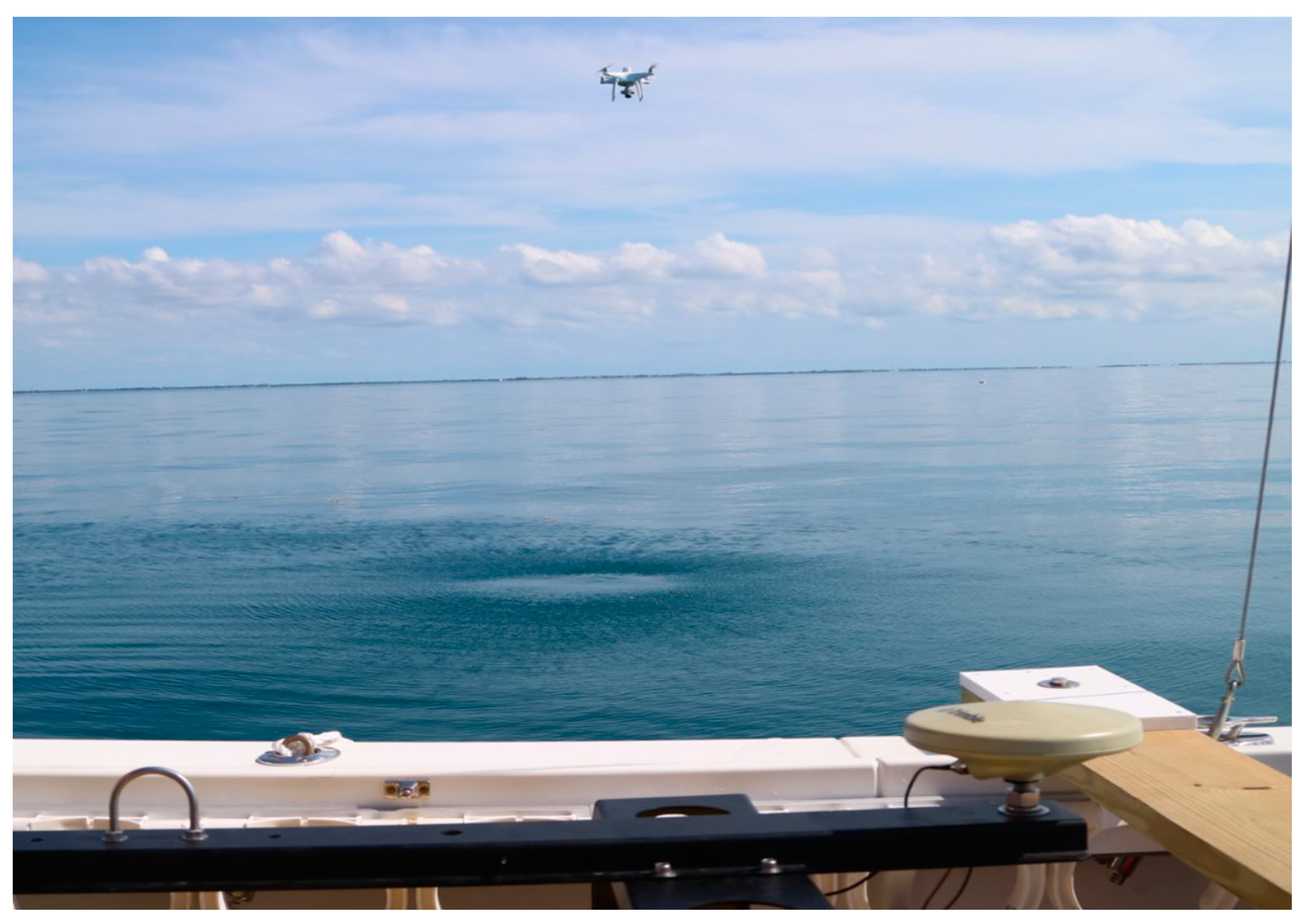
The imagery was collected with a DJI Phantom 4 Pro RTK (Figure 5). The remote aircraft has multi-frequency, multi-constellation, carrier-phase recording GNSS, which supports real-time kinematic (RTK) and post-processed kinematic (PPK) GNSS. For the purposes of this study, the remote aircraft trajectory was post-processed in the open-source GNSS software library, RTKLib [40]. The aircraft is equipped with a gimbal-mounted 20 MP (5472 × 3648 pixel) RGB camera. The focal length of the camera lens (actual, not 35 mm equivalent) is 8.6 mm, and the aperture is adjustable between f/2.8 and f/11. Due to the distance of the sites offshore (Figure 6), takeoff and landing were performed from a 7.6 m (25 ft) Parker dive boat owned and operated by the Mote Marine Laboratory. All flights were conducted at a flying height of 73 m above the water surface, resulting in a 2.0 cm ground sample distance (GSD) on the water surface.
It should be noted that there are several environmental and acquisition parameters that must be carefully selected to acquire good-quality UAS imagery of the seafloor. Specific challenges include sun glint, surface waves, and wind. These can be addressed, to some extent, through selection of suitable conditions (e.g., sun angle, water clarity) and acquisition parameters and procedures (e.g., use of a circular polarizing filter, orienting flightlines into and out of the sun). Rigorous testing of these parameters was beyond the scope of this study, but, to the extent possible, we adhered to recommendations published by our research group from a previous study [41]. Specific environmental parameters for the data acquisition are shown in Table 2.
One image for each of the two sites was chosen for performing SDB. The selection of appropriate images was nontrivial, and, in fact, turned out to be one of the most challenging practical aspects of this study. We sought images that would reflect different seafloor characteristics from one another. Additional considerations included (1) a wide enough range of depths to provide a robust test, (2) somewhat uniform water column and seafloor composition, such that the Stumpf algorithm would provide good results, (3) little sediment or plankton in the water column or on the water surface, (4) minimal sun glint, and (5) enough texture for structure-from-motion (SfM) photogrammetry software to be able to create georeferenced orthoimages from the raw images (such that our SDB was inherently georeferenced and the images were corrected for lens distortion). After manually analyzing dozens of images for two that would meet these (somewhat conflicting) criteria, the two images selected were EDR-47 and SiteC-75, both containing some reef (albeit different reef structures), sand, generally sloping bathymetry, and depth ranges of ~17 m. EDR-47 was acquired on 25 June 2022, while SiteC-75 was acquired one day earlier, on 24 June 2022.
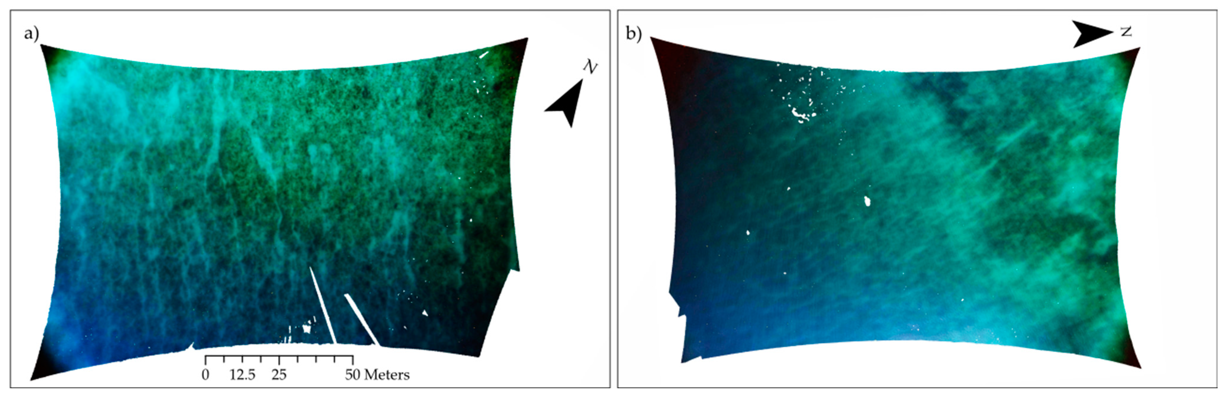
These two images were processed in Agisoft Metashape SfM software [42] to produce individual orthoimages (Figure 7), which served as the input to the SDB algorithm. It is important to note that the SfM step is, in general, unnecessary; the only requirements to use the SDB refraction correction procedure developed in this work are (a) the imagery needs to be georeferenced, and (b) it must be possible to compute radial image distances. The purpose of the SfM step in this study was simply to ensure good quality georeferencing and lens distortion correction to minimize sources of error unrelated to the refraction correction procedure. For a description of the general steps in an SfM workflow, interested readers are referred to [43,44].
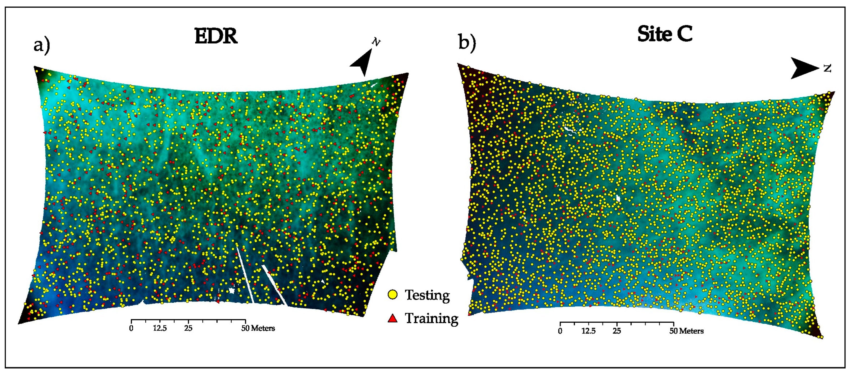
The reference data for this site are derived from the “2018–2019 NOAA NGS Topobathy Lidar DEM” collected after Hurricane Irma and obtained from NOAA’s Digital Coast. This dataset is referenced to NAD 83(2011) with UTM Zone 17N coordinates and NAVD88 (GEOID 12B) heights, in units of meters. The resolution of the DEM is 1 m. The data were acquired with a Riegl VQ-880-G+. The published vertical accuracy at a 95% confidence interval for the bathymetric lidar data was 11 cm, based on an accuracy assessment conducted by the service provider, Quantum Spatial (now NV5), in the shallow-water portions of the collection area. For the deeper portions of the site, the metadata states that the data were collected to meet Quality Level 2B of the National Coastal Mapping Strategy. Importantly, these data meet the ASPRS Positional Accuracy Standards for Digital Geospatial Data, 2nd Ed. requirement that reference data must be three times more accurate than the data being evaluated [45], A 20/80 training/testing split was used (i.e., 20% training, 80% testing). The locations of the training and testing samples for the two sites are shown in Figure 8.
There are two aspects of the reference data that merit discussion, as they may have had some impact on the SDB and assessed SDB accuracies. The first is that the training and testing samples were drawn from the same lidar dataset, although care was taken to ensure each consisted of an entirely separate set of points from the other. The second is that the spatial resolution of the lidar-derived DEM (1-m GSD) was much coarser than the UAS imagery. However, it is important to note that the goal of this study is not to evaluate the accuracy of SDB, but, rather, to assess the accuracy improvement enabled by incorporating refraction correction. Because both factors would tend to affect the un-refraction-corrected and refraction-corrected versions of the model equally, they should be of little consequence for evaluating the impacts of the refraction correction.
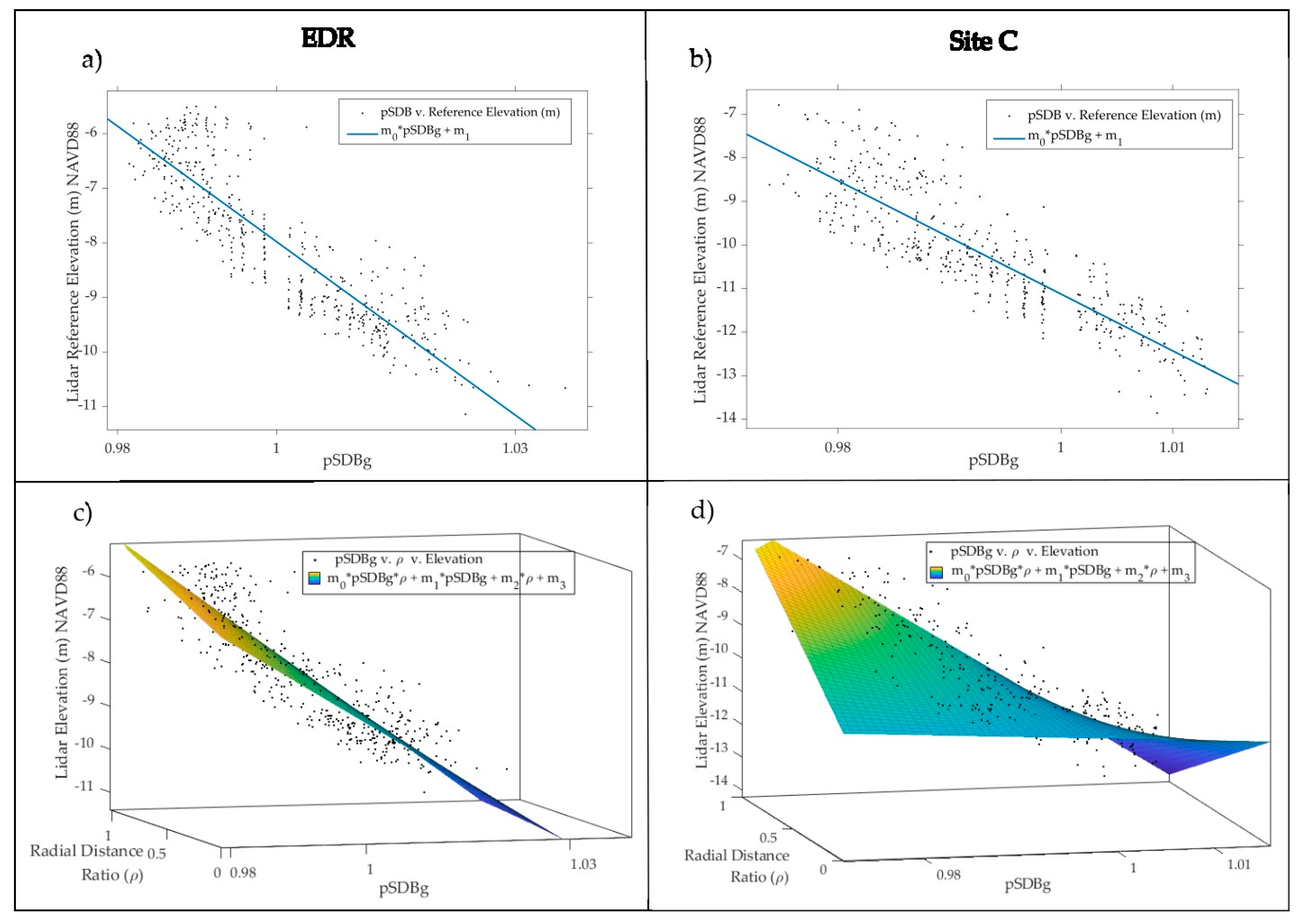
Both EDR-47 and SiteC-75 were processed using both the standard Stumpf algorithm and our modified version, incorporating the refraction correction terms. Both the standard Stumpf model and our refraction-corrected version were implemented in MATLAB (R2021a), with the multiple linear regression to solve for the parameters (m0 and m1 in the standard model, and m0–m4 in our version) performed using the MATLAB Curve Fitting Toolbox (Figure 9 and Table 3). As expected, the additional parameter improves the model fit. It is interesting to note the difference in the regression surfaces between the two photos, in which EDR is near-linear but Site C has a greater curvature. The potential overfitting at Site C, likely absorbing some other systematic error, has implications on the resulting model that becomes apparent during analysis (Figure 10 and Figure 11). The parameters generated from the regressions were then applied to the pSDBg and radial distance ratio raster datasets using ArcGIS, Raster Calculator. The outputs from each version of the model were compared to the reference data subset from the NOAA NGS airborne topobathymetric lidar dataset.
4. Results
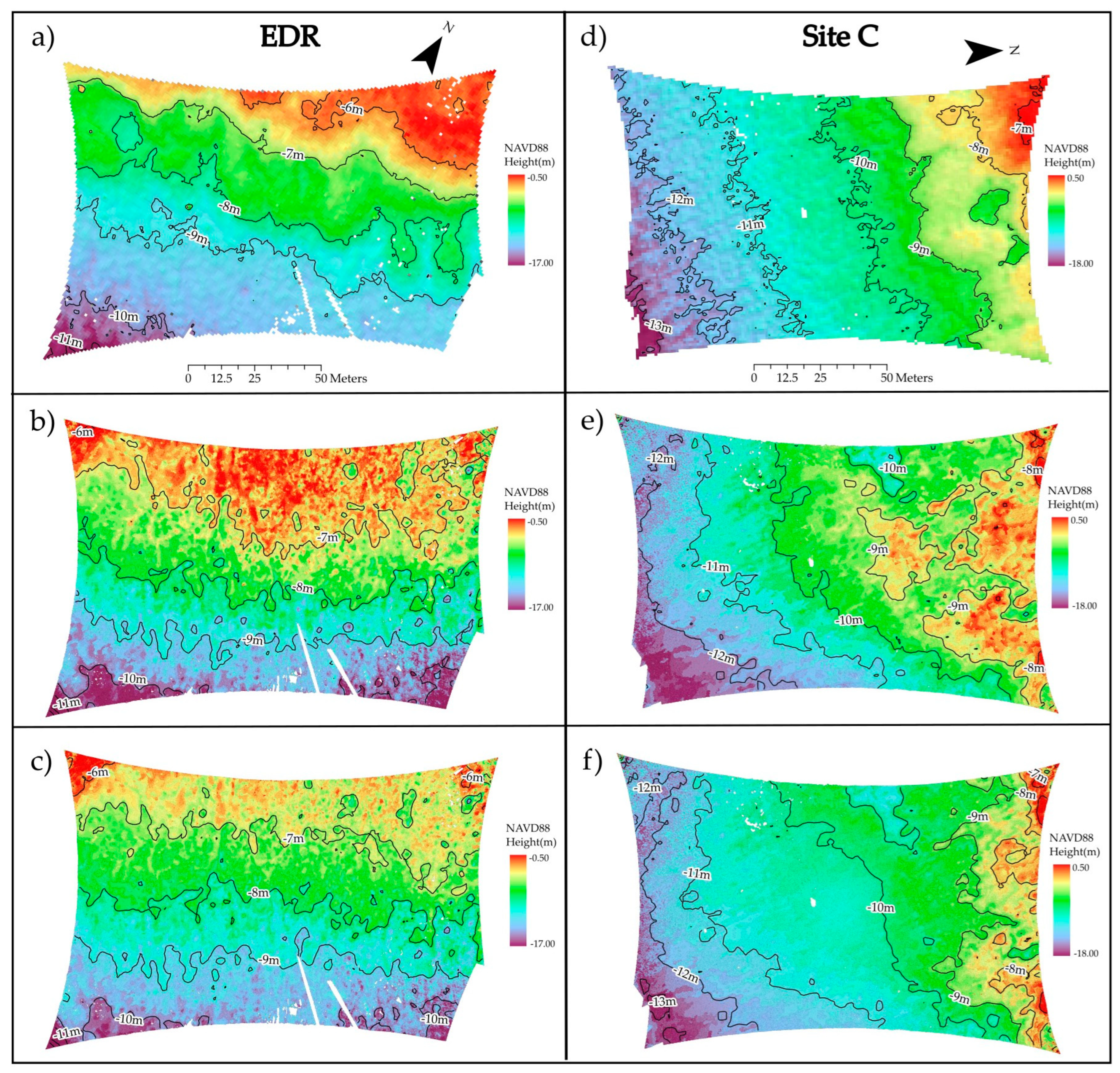
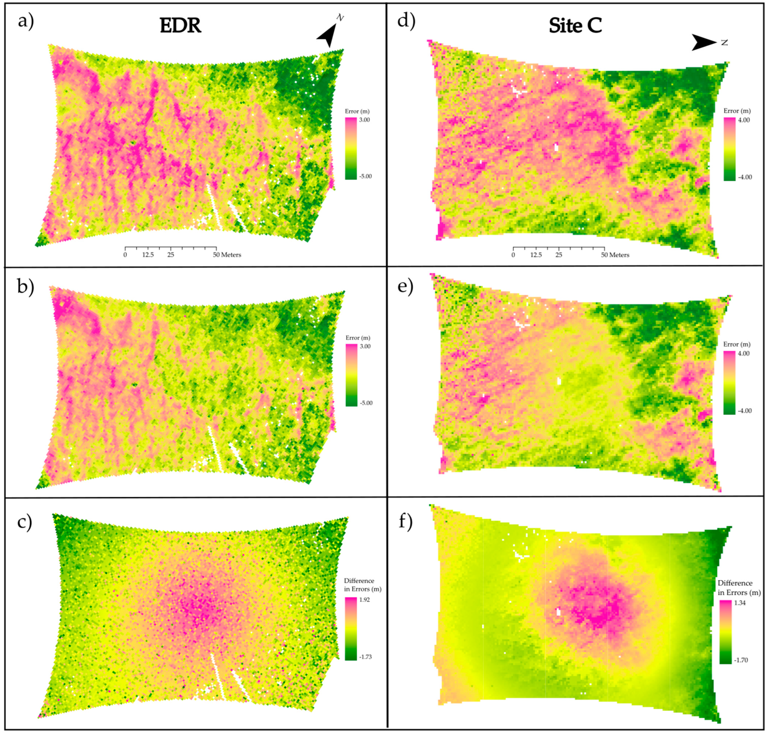
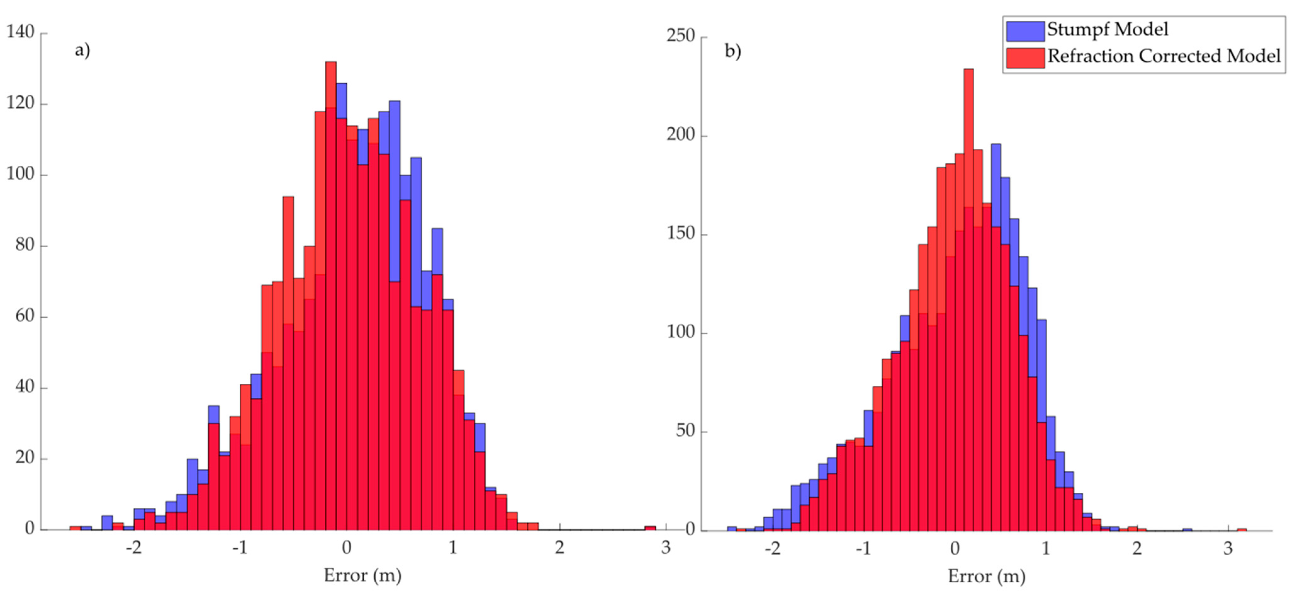
The results of comparing the output SDB bathymetric grids generated using both the standard Stumpf model and our refraction-corrected version are depicted in Figure 10, Figure 11 and Figure 12. Figure 10 shows in the top row the lidar-derived DEMs with overlaid contour lines for the two sites: EDR on the left, and Site C on the right. Below these are the bathymetric grids generated using both the standard Stumpf model (middle row) and our refraction-corrected version (bottom row), both also with contour lines overlaid. The errors (differences from reference data) from the two versions of the model are shown in Figure 11, with the top row of figures corresponding to the standard Stumpf model and the middle row corresponding to our refraction-corrected version. The bottom row depicts differences in errors between standard and refraction-corrected models for both sites. Figure 12 shows the error histograms for the two sites using both versions of the model.
The accuracy assessment statistics are summarized in Table 4. For both sites, the difference in MSE between the two datasets was found to be statistically significant at a significance level of α = 0.05, based on a one-sample t-test. Note that the t-test was performed on MSE, rather than RMSE, since the former is linear in squared error. Since the presence of systematic errors often manifests as a non-normal error distribution, a Lilliefors test for normality [46] was applied to the errors from the standard version of the Stumpf model and our refraction-corrected version. This test is applied to evaluate the null hypothesis that the data are drawn from a normal distribution when the mean and standard deviation are unknown, which is the typical case in assessing error distributions from an empirical accuracy assessment. We implemented the Lilliefors test using the MATLAB “lillietest” function.
5. Discussion
The results illustrate that the refraction-corrected version of the Stumpf algorithm led to improved results. For both images, the MSE was smaller using the refraction-corrected version of the model, with the difference in MSE being statistically significant, based on the results of the t-test. The reduction in bias (absolute value) was 75% for EDR and 46% for Site C, and the improvement in RMSE was 3 cm for EDR and 11 cm for Site C. In the case of EDR, the errors (differences from the reference data) fail the normality test (Lilliefors test) before the refraction correction and pass after the refraction correction. For Site C, both sets of errors fail the normality test, but visually, the error distribution for the refraction-corrected model is much closer to normal, and the skewness of the error distribution is reduced from −0.562 to −0.252. The importance of this finding lies in the fact that the presence of large systematic errors (such as those we would expect due to ignoring refraction correction) often manifests as non-normal error distributions [47,48]. A final indication that our refraction-corrected model is performing as expected is that the differences in errors (standard model minus refraction-corrected model), shown in Figure 11c,f display the expected radial pattern, because the refraction correction increases with the off-nadir angle, and, hence, with the radial image distance. Comparing 11c and 11f, one noticeable difference is that the EDR site appears to have more random errors, manifest in the speckled appearance of 11c as compared to 11f, which is smoother. The relative lack of symmetry in Figure 11f compared to Figure 11c indicates the presence of another systematic error, related to the location of the principal point and image tilt as well as the uneven brightness across the Site C image. While the cause of the greater random noise in the EDR SDB is unknown, it is important to note that the imagery for the two different sites were collected one day and ~37 km apart and under slightly different illumination, wind, wave, and water conditions. From Figure 7, it can be seen that the Site C image has a slightly smoother appearance, consistent with less random noise in the resultant SDB.
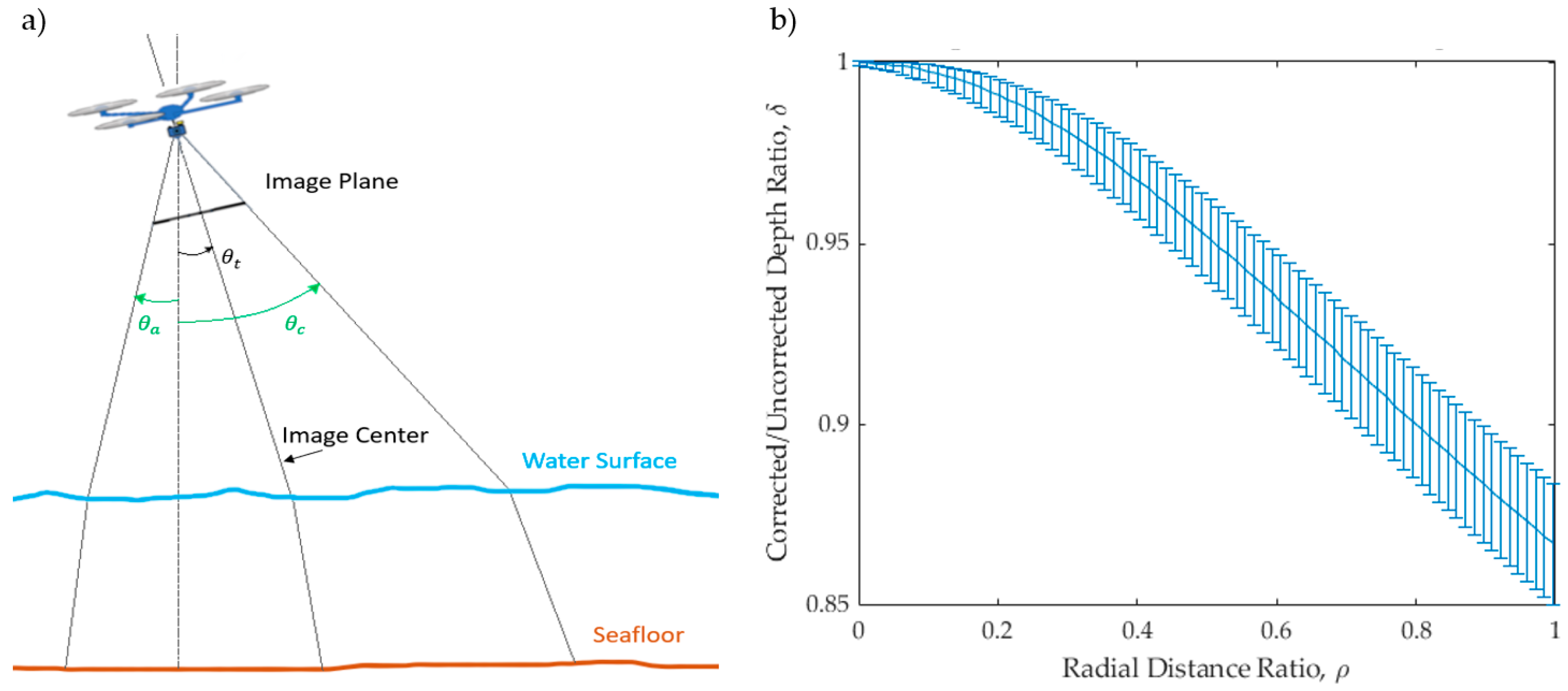
Returning to the simplifying assumptions underlying the refraction-corrected model, one that merits further discussion is the assumption that there is no image tilt. Even imagery intended to be vertical is typically not perfectly so, and, hence, the validity of this assumption could be called into question. Figure 13 shows the error bars on the refraction correction , if the image is assumed vertical when there is 3° of tilt. Even for this relatively large amount of tilt (for an image intended to be vertical), the maximum depth correction error at the outermost edges of the image is approximately ±1.5%, and the average error is approximately ±1.1%. For a more typical 1° tilt [30], the maximum depth correction error is approximately ±0.5%, and the average error is approximately ±0.4%. For reference, as reported by Agisoft Metashape [42], the tilts of EDR-47 and SiteC-75 were 0.957° and 0.738°, respectively. For the particular camera used in this study, roll would have the greatest error influence, since the rotation around the y-axis will either dip or raise the image along the longer dimension of the image.
The spatial distribution of the remaining errors in Figure 11b,e are best explained by factors unrelated to the refraction correction. Visually, the greatest remaining source of error with UAS bathymetry is the highly variable reflectance of the seafloor and cover. In general, areas of vegetation in the UAS SDB have a deep bias, while areas of sandy bottom have a shallow bias. The coral reef appears equally low in blue and green reflectance than the brighter areas of sand and therefore the low reflectance conditions are erroneously computed as deeper water.
It is also worth revisiting the requirements for the input to our refraction-corrected SDB model. Again, the SfM step is not required and was only applied in this study to improve the spatial accuracy and ensure that camera calibration was applied (and, hence, limit the influence of these nuisance parameters on the results). It is, however, necessary for the input imagery to be georeferenced in order to obtain georeferenced bathymetry as the output. With or without refraction correction, the spatial accuracy of the output bathymetry will be limited by the accuracy of the georeferencing. The other important requirement for the input to our procedure is that it must be possible to calculate radial image distances from the principal point. This is straightforward for an individual image, but it is extremely difficult in an orthomosaic generated from multiple, overlapping images. Hence, if orthorectification is performed on the input imagery, the input to the refraction-corrected SDB model should consist of individual orthoimages, rather than orthomosaics.
6. Conclusions
This study investigated refraction correction for SDB using imagery acquired using a small, commercially available UAS. The primary contributions of the study include (a) equations were developed for SDB refraction correction; (b) a simple-to-implement refraction correction procedure that consists of a modification of the well-known, widely used Stumpf algorithm was developed; and (c) the improvement achieved using the procedure was quantified. The difference in mean square error between the results of the standard model and our refraction-corrected version was found to be statistically significant at a significance level of α = 0.05. Additionally, the refraction correction reduced the bias in both study sites. For one of the sites, the errors failed a normality test before the refraction correction and passed the normality test after the correction, and for both sites, the error distribution was visually more normally distributed in the output, including the refraction correction terms. These findings support the conclusion that the refraction correction achieves the intended objective of reducing systematic errors in SDB, due to variable slant range through the water column. Equally importantly, it does so via a straightforward procedure that requires only the imagery and radial image distances as input. Our MATLAB code and data have been made available as Supplemental Materials, such that others can implement and assess the procedure.
Although the correction was tested on UAS imagery, there is no reason it could not be applied to SDB derived from imagery from other platforms, including conventional aircrafts and satellites. However, for satellite imagery, the corrections will be smaller, due to the smaller FOVs of the sensors. In terms of future work, an enhancement to the refraction correction developed in this study would be to further explore the cubic correction, rather than linear and radial image distance. Additionally, it would be interesting to evaluate the general method of refraction correction (i.e., inclusion of additional terms that are functions of radial image distance) with other SDB algorithms than the Stumpf algorithm.
A final recommendation for future work is to extend this study to include investigation of SDB from imagery that is not intended to be vertical. Most aerial imagery, including imagery acquired from both UAS and conventional aircraft, is intended to be vertical, and, hence, it was deemed appropriate to purposefully limit this scope of this study to vertical imagery. Furthermore, it was demonstrated that, for imagery intended to be vertical, typical image tilts of ~1° up to ~3° would introduce relatively small errors in the refraction correction. However, some high-resolution commercial satellite sensors acquire imagery with intentionally large off-pointing angles (e.g., 30°–45°). Although outside the scope of this study, further modifications to the model to support such oblique imagery should, in theory, be feasible.
Supplementary Materials
The following supporting information can be downloaded at: https://www.mdpi.com/article/10.3390/rs15143635/s1. The data presented in this study are available in Supplementary Materials, including original photos (Figures S1 and S2), orthoimages (Figures S3 and S4), radial distance ratio orthoimages (Figures S5 and S6), test data points (Table S1), error values (Table S2), and MATLAB scripts ‘radialDist_slant_correction.m’ used to generate the analytical models, ‘RadialRatio_Image.m’ for generating the radial ratio image, and ‘lillie_normalitytest.m’ for error analysis.
Author Contributions
Conceptualization, S.E.L. and C.E.P.; methodology, S.E.L. and C.E.P.; software, S.E.L.; validation, S.E.L. and C.E.P.; formal analysis, S.E.L. and C.E.P.; investigation, S.E.L.; resources, C.E.P.; data curation, S.E.L.; writing—original draft preparation, S.E.L.; writing—review and editing, S.E.L. and C.E.P.; visualization, S.E.L.; supervision, C.E.P.; project administration, C.E.P.; funding acquisition, C.E.P. All authors have read and agreed to the published version of the manuscript.
Funding
This research was funded by the United States National Oceanic and Atmospheric Administration (NOAA) Grant NA20NOS4000196 to the University of New Hampshire, Joint Hydrographic Center, and subaward L0125 to Oregon State University.
Data Availability Statement
The bathymetric lidar data used in this study are available on NOAA’s Digital Coast: https://coast.noaa.gov/digitalcoast/, accessed on 21 June 2022. The orthoimages generated in the study are being made available on ScholarsArchive@OSU, Oregon State University’s digital service for disseminating scholarly work.
Acknowledgments
We would like to gratefully acknowledge Jenn Dijkstra, UNH PI of the multi-modal marine resource mapping project in the Florida Keys, under which the data for this study were collected. We would also like to acknowledge Chase Simpson, Instructor of Geomatics at Oregon State University, LT Matt Sharr and Gretchen Imahori of NOAA, and Erich Bartels, Kyle Knoblock, and Ian Combs of Mote Marine Laboratory.
Conflicts of Interest
The authors declare no conflict of interest.
References
- Moore, J.G. The determination of the depths and extinction coefficients of shallow water by air photography using colour filters. Philosophical Trans. Royal Soc. London Ser. A Math. Phys. Sci. 1947, 240, 163–217. [Google Scholar]
- Tewinkel, G.C. Water depths from aerial photographs. Photogramm. Eng. 1963, 29, 1037–1042. [Google Scholar]
- Polcyn, F.C.; Lyzenga, D.R. Remote Bathymetry and Shoal Detection with ERTS: ERTS Water Depth. 1975. Available online: https://ntrs.nasa.gov/api/citations/19750014800/downloads/19750014800.pdf (accessed on 21 June 2022).
- Brewer, R.K. Project planning and field support for NOS photobathymetry. Int. Hydrogr. Rev. 1979, 56, 55–66. [Google Scholar]
- Brown, R.M.; Zied, A.; Arnone, R.; Townsend, F.; Scarpace, F. Water Penetration Photogrammetry. In Feasibility and Evaluation Study; Naval Ocean Research and Development Activity Stennis: Hancock County, MS, USA, 1983; Volume 1. [Google Scholar]
- Zhang, C. Applying data fusion techniques for benthic habitat mapping and monitoring in a coral reef ecosystem. ISPRS J. Photogramm. Remote Sens. 2015, 104, 213–223. [Google Scholar] [CrossRef]
- Hedley, J.D.; Roelfsema, C.; Brando, V.; Giardino, C.; Kutser, T.; Phinn, S.; Mumby, P.J.; Barrilero, O.; Laporte, J.; Koetz, B. Coral reef applications of Sentinel-2: Coverage, characteristics, bathymetry and benthic mapping with comparison to Landsat 8. Remote. Sens. Environ. 2018, 216, 598–614. [Google Scholar] [CrossRef]
- Purkis, S.J.; Gleason, A.C.; Purkis, C.R.; Dempsey, A.C.; Renaud, P.G.; Faisal, M.; Saul, S.; Kerr, J.M. High-resolution habitat and bathymetry maps for 65,000 sq. km of Earth’s remotest coral reefs. Coral Reefs 2019, 38, 467–488. [Google Scholar] [CrossRef] [Green Version]
- Misra, A.; Ramakrishnan, B. Assessment of coastal geomorphological changes using multi-temporal Satellite-Derived Bathymetry. Cont. Shelf Res. 2020, 207, 104213. [Google Scholar] [CrossRef]
- Herrmann, J.; Magruder, L.A.; Markel, J.; Parrish, C.E. Assessing the ability to quantify bathymetric change over time using solely satellite-based measurements. Remote Sens. 2022, 14, 1232. [Google Scholar] [CrossRef]
- Pe’eri, S.; Madore, B.; Nyberg, J.; Snyder, L.; Parrish, C.; Smith, S. Identifying bathymetric differences over Alaska’s North Slope using a satellite-derived bathymetry multi-temporal approach. J. Coastal Res. 2016, 76, 56–63. [Google Scholar] [CrossRef]
- Mavraeidopoulos, A.K.; Pallikaris, A.; Oikonomou, E. Satellite derived bathymetry (SDB) and safety of navigation. Int. Hydrogr. Rev. 2017, 17, 7–20. [Google Scholar]
- Chénier, R.; Faucher, M.A.; Ahola, R. Satellite-derived bathymetry for improving Canadian Hydrographic Service charts. ISPRS Int. J. Geo Inf. 2018, 7, 306. [Google Scholar] [CrossRef] [Green Version]
- Guenther, G.C. Airborne lidar bathymetry. In Digital Elevation Model Technologies and Applications: The DEM Users Manual; ASPRS Publications: Baton Rouge, LA, USA, 2007; Volume 2, pp. 253–320. [Google Scholar]
- Dietrich, J.T. Bathymetric structure-from-motion: Extracting shallow stream bathymetry from multi-view stereo photogrammetry. Earth Surf. Process. Landf. 2017, 42, 355–364. [Google Scholar] [CrossRef]
- Mancini, S.; Olsen, R.C.; Abileah, R.; Lee, K.R. Automating nearshore bathymetry extraction from wave motion in satellite optical imagery. In Proceedings of the SPIE Algorithms and Technologies for Multispectral, Hyperspectral, and Ultraspectral Imagery XVIII, Baltimore, MD, USA, 23–27 April 2012; Volume 8390, pp. 206–217. [Google Scholar]
- Abileah, R.; Blot, J.Y. Bathymetry of the Golfe d’Arguin, Mauritania, derived with the moderate resolution Sentinel-2 satellites. In Proceedings of the IEEE OCEANS 2021: San Diego–Porto, San Diego, CA, USA, 20–23 September 2021; pp. 1–7. [Google Scholar]
- Lyzenga, D.R. Passive remote sensing techniques for mapping water depth and bottom features. Appl. Opt. 1978, 17, 379–383. [Google Scholar] [CrossRef] [PubMed]
- Stumpf, R.P.; Holderied, K.; Sinclair, M. Determination of water depth with high-resolution satellite imagery over variable bottom types. Limnol. Oceanogr. 2003, 48, 547–556. [Google Scholar] [CrossRef]
- Caballero, I.; Stumpf, R.P. Towards routine mapping of shallow bathymetry in environments with variable turbidity: Contribution of Sentinel-2A/B satellites mission. Remote Sens. 2020, 12, 451. [Google Scholar] [CrossRef] [Green Version]
- Muzirafuti, A.; Crupi, A.; Lanza, S.; Barreca, G.; Randazzo, G. Shallow water bathymetry by satellite image: A case study on the coast of San Vito Lo Capo Peninsula, Northwestern Sicily, Italy. In Proceedings of the 2019 IMEKO TC-19 International Workshop on Metrology for the Sea, Genoa, Italy, 3–5 October 2019. [Google Scholar]
- Ashphaq, M.; Srivastava, P.K.; Mitra, D. Review of near-shore satellite derived bathymetry: Classification and account of five decades of coastal bathymetry research. J. Ocean Eng. Sci. 2021, 6, 340–359. [Google Scholar] [CrossRef]
- Slocum, R.K.; Parrish, C.E.; Simpson, C.H. Combined geometric-radiometric and neural network approach to shallow bathymetric mapping with UAS imagery. ISPRS J. Photogramm. Remote Sens. 2020, 169, 351–363. [Google Scholar] [CrossRef]
- Maas, H.G. On the accuracy potential in underwater/multimedia photogrammetry. Sensors 2015, 15, 18140–18152. [Google Scholar]
- Parrish, C.E.; Magruder, L.A.; Neuenschwander, A.L.; Forfinski-Sarkozi, N.; Alonzo, M.; Jasinski, M. Validation of ICESat-2 ATLAS bathymetry and analysis of ATLAS’s bathymetric mapping performance. Remote Sens. 2019, 11, 1634. [Google Scholar] [CrossRef] [Green Version]
- Agrafiotis, P.; Karantzalos, K.; Georgopoulos, A.; Skarlatos, D. Correcting image refraction: Towards accurate aerial image-based bathymetry mapping in shallow waters. Remote Sens. 2020, 12, 322. [Google Scholar] [CrossRef] [Green Version]
- Mandlburger, G.; Kölle, M.; Nübel, H.; Soergel, U. BathyNet: A deep neural network for water depth mapping from multispectral aerial images. PFG J. Photogramm. Remote Sens. Geoinf. Sci. 2021, 9, 71–89. [Google Scholar] [CrossRef]
- Rossi, L.; Mammi, I.; Pelliccia, F. UAV-Derived Multispectral Bathymetry. Remote Sens. 2020, 12, 3897. [Google Scholar] [CrossRef]
- Klemm, A.; Pe’eri, S.; Freire, R.; Nyberg, J.; Smith, S. Nautical Chart Adequacy Evaluation Using Publicly-Available Data. In Proceedings of the U.S. Hydrographic Conference, National Harbor, MD, USA, 16–19 March 2015. [Google Scholar]
- Wolf, P.R.; Dewitt, B.A.; Wilkinson, B.E. Elements of Photogrammetry with Applications in GIS; McGraw-Hill Education: New York City, NY, USA, 2014. [Google Scholar]
- Babbel, B.J.; Parrish, C.E.; Magruder, L.A. ICESat-2 elevation retrievals in support of satellite-derived bathymetry for global science applications. Geophys. Res. Lett. 2021, 48, e2020GL090629. [Google Scholar] [CrossRef] [PubMed]
- Casal, G.; Monteys, X.; Hedley, J.; Harris, P.; Cahalane, C.; McCarthy, T. Assessment of empirical algorithms for bathymetry extraction using Sentinel-2 data. Int. J. Remote Sens. 2019, 40, 2855–2879. [Google Scholar] [CrossRef]
- Traganos, D.; Poursanidis, D.; Aggarwal, B.; Chrysoulakis, N.; Reinartz, P. Estimating satellite-derived bathymetry (SDB) with the google earth engine and sentinel-2. Remote Sens. 2018, 10, 859. [Google Scholar] [CrossRef] [Green Version]
- Reguero, B.G.; Beck, M.W.; Agostini, V.N.; Kramer, P.; Hancock, B. Coral reefs for coastal protection: A new methodological approach and engineering case study in Grenada. J. Environ. Manag. 2018, 210, 146–161. [Google Scholar] [CrossRef]
- Geyman, E.C.; Maloof, A.C. A simple method for extracting water depth from multispectral satellite imagery in regions of variable bottom type. Earth Space Sci. 2019, 6, 527–537. [Google Scholar] [CrossRef]
- Hsu, H.J.; Huang, C.Y.; Jasinski, M.; Li, Y.; Gao, H.; Yamanokuchi, T.; Wang, C.G.; Chang, T.M.; Ren, H.; Kuo, C.Y.; et al. A semi-empirical scheme for bathymetric mapping in shallow water by ICESat-2 and Sentinel-2: A case study in the South China Sea. ISPRS J. Photogramm. Remote Sens. 2021, 178, 1–9. [Google Scholar] [CrossRef]
- Parrish, C.E.; Magruder, L.; Herzfeld, U.; Thomas, N.; Markel, J.; Jasinski, M.; Imahori, G.; Herrmann, J.; Trantow, T.; Borsa, A.; et al. ICESat-2 Bathymetry: Advances in Methods and Science. In Proceedings of the IEEE OCEANS, Hampton Roads, VA, USA, 17–20 October 2022; pp. 1–6. [Google Scholar]
- Sharr, M.B.; Parrish, C.E.; Jung, J. Classifying Valid and Erroneous Depths in Satellite Derived Bathymetry with Random Forest. ISPRS J. Photogramm. Remote Sens. 2023; in review. [Google Scholar]
- Bartels, E.; (Mote Marine Laboratory, Summerland Key, FL, USA). Personal communication, 2023.
- Takasu, T.; Yasuda, A. Development of the low-cost RTK-GPS receiver with an open source program package RTKLIB. In Proceedings of the International Symposium on GPS/GNSS, Seogwipo-si, Republic of Korea, 4–6 November 2009; International Convention Center Jeju Korea: Seogwipo-si, Republic of Korea, 2009; Volume 1, pp. 1–6. [Google Scholar]
- Slocum, R.K.; Wright, W.; Parrish, C.; Costa, B.; Sharr, M.; Battista, T.A. Guidelines for Bathymetric Mapping and Orthoimage Generation using sUAS and SfM, An Approach for Conducting Nearshore Coastal Mapping. In NOAA Technical Memorandum NOS NCCOS 265; National Ocean Service (NOS): Silver Spring, MD, USA; National Centers for Coastal Ocean Science (NCCOS): Silver Spring, MD, USA; NOAA: Silver Spring, MD, USA, 2019. [Google Scholar] [CrossRef]
- Over, J.S.; Ritchie, A.C.; Kranenburg, C.J.; Brown, J.A.; Buscombe, D.D.; Noble, T.; Sherwood, C.R.; Warrick, J.A.; Wernette, P.A. Processing Coastal Imagery with Agisoft Metashape Professional Edition, Version 1.6—Structure from Motion Workflow Documentation; US Geological Survey: Reston, VA, USA, 2021.
- Fonstad, M.A.; Dietrich, J.T.; Courville, B.C.; Jensen, J.L.; Carbonneau, P.E. Topographic structure from motion: A new development in photogrammetric measurement. Earth Surf. Process. Landf. 2013, 38, 421–430. [Google Scholar] [CrossRef] [Green Version]
- Mancini, F.; Dubbini, M.; Gattelli, M.; Stecchi, F.; Fabbri, S.; Gabbianelli, G. Using unmanned aerial vehicles (UAV) for high-resolution reconstruction of topography: The structure from motion approach on coastal environments. Remote Sens. 2013, 5, 6880–6898. [Google Scholar] [CrossRef] [Green Version]
- American Society for Photogrammetry and Remote Sensing (ASPRS). Positional Accuracy Standards for Digital Geospatial Data, 2nd ed.; ASPRS Publications: Baton Rouge, LA, USA, 2023. [Google Scholar]
- Lilliefors, H.W. On the Kolmogorov-Smirnov test for normality with mean and variance unknown. J. Am. Stat. Assoc. 1967, 62, 399–402. [Google Scholar] [CrossRef]
- Aguilar, F.J.; Mills, J.P. Accuracy assessment of LiDAR-derived digital elevation models. Photogramm. Rec. 2008, 23, 148–169. [Google Scholar] [CrossRef]
- DeWitt, J.D.; Warner, T.A.; Conley, J.F. Comparison of DEMS derived from USGS DLG, SRTM, a statewide photogrammetry program, ASTER GDEM and LiDAR: Implications for change detection. GIScience Remote Sens. 2015, 52, 179–197. [Google Scholar] [CrossRef]
Figure 1.
Concept of SDB refraction correction. The difference between slant range and depth increases with increasing off-nadir angle, θ, and, correspondingly, with increasing image radial distance, r.
Figure 1.
Concept of SDB refraction correction. The difference between slant range and depth increases with increasing off-nadir angle, θ, and, correspondingly, with increasing image radial distance, r.

Figure 2.
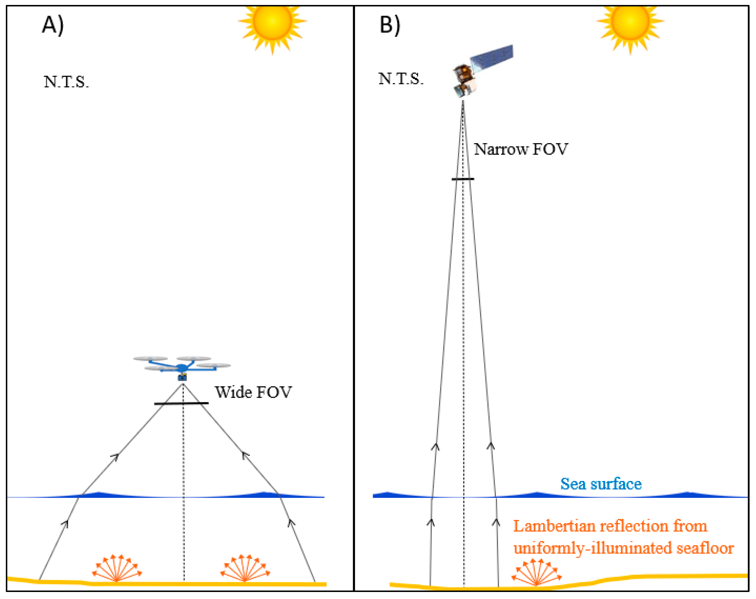
Greater variation in off-nadir angles with wide-FOV camera on UAS (A) than on narrow-FOV satellite sensors (B). Assuming the seafloor is uniformly illuminated within the image footprint, and that the reflection from the seafloor is Lambertian, it suffices to consider only the upwelling radiance of light reflected from the seafloor.
Figure 2.
Greater variation in off-nadir angles with wide-FOV camera on UAS (A) than on narrow-FOV satellite sensors (B). Assuming the seafloor is uniformly illuminated within the image footprint, and that the reflection from the seafloor is Lambertian, it suffices to consider only the upwelling radiance of light reflected from the seafloor.

Figure 3.
Geometry of SDB refraction correction for vertical aerial imagery.

Figure 4.
Relationship between depth correction, , and relative radial distance, , using camera parameters for the UAS camera used in this study (see description in Methods).
Figure 4.
Relationship between depth correction, , and relative radial distance, , using camera parameters for the UAS camera used in this study (see description in Methods).

Figure 5.
UAS image acquisition over Florida Keys project site with Phantom 4 Pro. In the foreground is the starboard gunwale of the Mote Marine Laboratory dive boat from which takeoff and landing were performed.
Figure 5.
UAS image acquisition over Florida Keys project site with Phantom 4 Pro. In the foreground is the starboard gunwale of the Mote Marine Laboratory dive boat from which takeoff and landing were performed.

Figure 6.
Project sites in the Florida Keys, USA.

Figure 7.
Orthoimages generated for the two UAS images: (a) EDR-47, and (b) SiteC-75. Blank white areas of the orthoimages are where the SfM reconstruction failed, due to floating algae or lack of sufficient seafloor texture. Both sites contain a mixture of reef (darker green) and sand (lighter) areas. The bowed edges of the orthoimages are a result of lens distortion, and the lower-intensity values near the image corners are a result of vignetting.

Figure 8.
Locations of testing samples (yellow circles) and training samples (red triangles) randomly drawn from the 2018–2019 NOAA NGS topobathymetric lidar dataset for the EDR site (a) and Site C (b). Although both training and testing samples were drawn from the same reference dataset, they were kept entirely separate from one another until the final analysis step of comparing the standard and refraction-corrected versions of the model.

Figure 9.
Regression lines and surfaces for the standard Stumpf model and our refraction-corrected version: (a) regression line from standard Stumpf model for EDR; (b) regression line from standard Stumpf model for Site C; (c) regression surface from our refraction-corrected model for EDR; (d) regression surface from our refraction-corrected model for Site C.

Figure 10.
Reference data and SDB without and with refraction-correction for the two sites: (a) lidar reference data for EDR (clipped to orthoimage area); (b) standard Stumpf model SDB for EDR; (c) refraction-correction model SDB for EDR; (d) lidar reference data for Site C (clipped to orthoimage area); (e) standard Stumpf model SDB for Site C; and (f) refraction-corrected SDB for Site C.

Figure 11.
Errors (model minus reference data) for both sites: (a) standard Stumpf model error for EDR; (b) refraction-corrected model error for EDR; (c) differences in errors between standard and refraction-corrected models for EDR; (d) standard Stumpf model error for Site C; (e) refraction-corrected model error for Site C; (f) differences in errors between standard and refraction-corrected models for Site C.

Figure 12.
Error distributions from standard model (blue) and refraction corrected model (red) for EDR (a) and Site C (b), based on comparisons of the SDB DEMs against the lidar reference data.
Figure 12.
Error distributions from standard model (blue) and refraction corrected model (red) for EDR (a) and Site C (b), based on comparisons of the SDB DEMs against the lidar reference data.

Figure 13.
Effects of uncorrected image tilt: (a) graphical illustration of uncorrected image tilt; (b) refraction correction with corresponding error bars (corresponding to 3° of uncorrected image tilt) as a function of radial distance ratio.
Figure 13.
Effects of uncorrected image tilt: (a) graphical illustration of uncorrected image tilt; (b) refraction correction with corresponding error bars (corresponding to 3° of uncorrected image tilt) as a function of radial distance ratio.


Table 1.
Comparison of estimated relative depth errors resulting from ignoring refraction correction for satellite imagery and a large FOV UAS camera.
Table 1.
Comparison of estimated relative depth errors resulting from ignoring refraction correction for satellite imagery and a large FOV UAS camera.
| Sensor | Platform | Field of View | Max Relative Depth Error from Ignoring Refraction Correction (Assuming Vertical Image) | Mean Relative Depth Error from Ignoring Refraction Correction (Assuming Vertical Image) |
|---|---|---|---|---|
| Operational Land Imager (OLI) | Landsat 8–9 satellites | 15° | 0.5% | 0.2% |
| Multispectral Instrument (MSI) | Sentinel-2A and -2B satellites | 21° | 0.9% | 0.3% |
| DJI Phantom 4 Pro integrated camera | UAS | 84° | 13.3% | 5.4% |
Table 2.
Environmental parameters during data acquisition. The wave height, wind, humidity, and temperature data were obtained from the National Data Buoy Center, using the closest buoy. The Kd(490) and SPM data were obtained from the NOAA STAR Ocean Color viewer (OCView) web portal and computed from Visible Infrared Imaging Radiometer Suite (VIIRS) data. Only the 24 June 2022 data were used from OCView, because the sites were cloud covered at the specific time of the satellite overpass on 25 June. The solar altitude and azimuth were obtained from an online solar calculator.
| Parameter | EDR | Site C |
|---|---|---|
| Solar altitude | 38°–43° | 38°–43° |
| Solar azimuth | 78°–80° | 78°–80° |
| Kd(490) (diffuse attenuation coefficient of downwelling irradiance at 490 nm) | 0.106 m−1 (Note: based on data from previous day) | 0.110 m−1 |
| SPM (suspended particulate matter) | 0.363 mg/L (Note: based on data from previous day) | 0.456 mg/L |
| Significant wave height | 0.20 m | 0.18–0.19 m |
| Wind speed | 1.6 m/s | 1.4 m/s |
| Atmospheric pressure | 1017.2 hPa | 1015.6 hPa |
| Humidity | 68% | 66% |
| Temperature | 27.9 °C | 27.5 °C |
Table 3.
Fit statistics of the regression lines from the standard Stumpf models and the regression surfaces from the refraction-corrected models.
Table 3.
Fit statistics of the regression lines from the standard Stumpf models and the regression surfaces from the refraction-corrected models.
| EDR (Standard) | EDR (Corrected) | Site C (Standard) | Site C (Corrected) | |
|---|---|---|---|---|
| SSE (m) | 196.9 | 172.4 | 242 | 165.7 |
| R2 | 0.79 | 0.81 | 0.75 | 0.83 |
| RMSE (m) | 0.640 | 0.600 | 0.718 | 0.596 |
Table 4.
Results from standard Stumpf algorithm and our version, incorporating the refraction-correction terms.
Table 4.
Results from standard Stumpf algorithm and our version, incorporating the refraction-correction terms.
| Standard Model: EDR-47 | Refraction-Corrected Model: EDR-47 | Standard Model: SiteC-75 | Refraction-Corrected Model: SiteC-75 | |
|---|---|---|---|---|
| Number of samples, N | 1947 | 1947 | 2963 | 2963 |
| RMSE (m) | 0.694 | 0.663 | 0.735 | 0.629 |
| Bias, μ (m) | 0.069 | 0.017 | 0.024 | −0.013 |
| Standard deviation, σ (m) | 0.561 | 0.538 | 0.734 | 0.629 |
| Mean squared error (MSE) (m2) | 0.481 | 0.440 | 0.540 | 0.396 |
| Skewness of error distribution | −0.534 | −0.135 | −0.562 | −0.252 |
| Error distribution passes normality test (Y/N) | No | Yes | No | No |
| Difference in MSE is statistically significant (Y/N) | Yes | Yes | ||
Disclaimer/Publisher’s Note: The statements, opinions and data contained in all publications are solely those of the individual author(s) and contributor(s) and not of MDPI and/or the editor(s). MDPI and/or the editor(s) disclaim responsibility for any injury to people or property resulting from any ideas, methods, instructions or products referred to in the content. |
© 2023 by the authors. Licensee MDPI, Basel, Switzerland. This article is an open access article distributed under the terms and conditions of the Creative Commons Attribution (CC BY) license (https://creativecommons.org/licenses/by/4.0/).
Share and Cite
MDPI and ACS Style
Lambert, S.E.; Parrish, C.E. Refraction Correction for Spectrally Derived Bathymetry Using UAS Imagery. Remote Sens. 2023, 15, 3635. https://doi.org/10.3390/rs15143635
AMA Style
Lambert SE, Parrish CE. Refraction Correction for Spectrally Derived Bathymetry Using UAS Imagery. Remote Sensing. 2023; 15(14):3635. https://doi.org/10.3390/rs15143635
Chicago/Turabian StyleLambert, Selina E., and Christopher E. Parrish. 2023. "Refraction Correction for Spectrally Derived Bathymetry Using UAS Imagery" Remote Sensing 15, no. 14: 3635. https://doi.org/10.3390/rs15143635
Note that from the first issue of 2016, this journal uses article numbers instead of page numbers. See further details here.