
On-Orbit Calibration and Wet Tropospheric Correction of HY-2C Correction Microwave Radiometer

1
Key Laboratory of Microwave Remote Sensing Technology, National Space Science Center, Chinese Academy of Sciences, Beijing 100190, China
2
University of Chinese Academy of Sciences, Beijing 100040, China
*
Author to whom correspondence should be addressed.
Remote Sens. 2023, 15(14), 3633; https://doi.org/10.3390/rs15143633
Submission received: 7 June 2023
/
Revised: 18 July 2023
/
Accepted: 18 July 2023
/
Published: 21 July 2023
(This article belongs to the Special Issue Remote Sensing Applications in Ocean Observation II)
Abstract
:HY-2C is the third satellite in China’s ocean dynamic environment satellite series, and carries a correction microwave radiometer (CMR) to correct the wet tropospheric path delay for the aligned radar altimeter. To effectively use the brightness temperatures (TB) of CMR to retrieve path delay, an on-orbit calibration effort is required. In this study, an antenna pattern correction (APC) method and a neural network method are used to perform an on-orbit calibration for CMR’s antenna temperatures and a model based on the Whale Optimization Algorithm (WOA), Levenberg–Marquardt (LM) algorithm, and Back-Propagation neural network (WOA–LM–BP) has been proposed to retrieve the wet tropospheric correction (WTC) of CMR. The on-orbit calibration results, compared with the simulated brightness temperatures calculated by the radiative transfer model (RTM), have shown that compared with the APC method, the neural network method can almost eliminate the latitude variation, and the total bias and standard deviation of the on-orbit calibrated TB at all channels have obviously decreased. The retrieved WTC results also have shown that the retrieved WTC of CMR has a good agreement with the corresponding ones from the model-derived WTC and Jason-3.
1. Introduction
Radar altimeter plays an indispensable role in the precision of Sea Surface Height (SSH) measurements, which have a great impact on the global ocean and climate study. The radar altimeter measures the SSH by the echo time between the satellite and the ocean surface. However, due to the comprehensiveness and complexity of the ocean dynamic environment, the spatial and temporal distribution of water vapor and cloud liquid water content is uneven, which introduces the wet troposphere path delay for the radar altimeter [1,2]. Generally, the wet troposphere path delay will lead to a 3~50 cm uncertainty error for SSH measurements with radar altimetry, which is one of the major error sources in radar altimetry applications.
In the past few decades, the passive microwave radiometers installed on the satellites have been recognized as the most accurate mean to measure the wet tropospheric correction (WTC) in most altimetric missions [3], such as the microwave radiometers (MWR) deployed on the Earth Remote Sensing (ERS) series satellites and Sentinel series satellites, the Topex/Poseidon microwave radiometer (TMR), the Jason microwave radiometer (JMR), the advanced microwave radiometer (AMR), and the calibration microwave radiometer (CMR) of the HY series satellites [4]. HY-2C is the third ocean dynamic environment monitoring satellite after HY-2A and HY-2B and was successfully launched by the Chinese National Satellite Ocean Application Service (NSOAS), the Ministry of Natural Resources (MNR) of China on 21 September 2020. A three-frequency nadir-viewing CMR, operating at 18.7 GHz, 23.8 GHz, and 37 GHz, was designed to measure WTC for the aligned HY-2C radar altimeter. The three frequencies were chosen for their sensibility to sea surface roughness or equivalence to wind speed (18.7 GHz), atmospheric water vapor (23.8 GHz), and atmospheric liquid water (37 GHz) [5]. By combing the different measured brightness temperatures (the on-orbit main-beam brightness temperatures of the microwave radiometer’s antenna, also referred to as TB) of CMR, the WTC of the radar altimeter can be determined with a retrieval algorithm; therefore, the accuracy of the measured brightness temperatures has been a matter of interest of several studies.
Generally, there are two main methods widely used for calculating or evaluating the on-orbit TB: simultaneous nadir overpass (SNOs) and observation minus background simulation (OMB). Ideally, when identical radiometers deployed on different satellites simultaneously observe the same Earth target, the observed TB should be identical; any difference would be caused by relative calibration discrepancies between the supposedly identical radiometers. The SNO method aims to minimize the measured TB differences between a pair of radiometers by utilizing the same place at the same time of near-nadir intersection observations [6]. The advantage of the SNO method is that it directly establishes the function between the sensor of interest (SOI) and the sensor reference standard (SRS). While this method has latitude limitation and needs to have relatively small time differences, the calibration accuracy and stability of the SOI is easily affected by the SRS [7,8]. The OMB method is a common metric used to quantify the difference between the observed TB and the background brightness temperature at a given frequency, time, and location. There are many commonly adopted background brightness temperatures, such as the Amazon forest whose surface target has relatively stable characteristics [9,10], and the simulated brightness temperatures from the radiative transfer model (RTM) with various atmospheric profiles and surface parameters [10,11]. Although the OMB method overlooks the real characteristics of the radiometers to some extent, and the calibration results are affected by the background field parameters and the accuracy of the RTM, this method can obtain a large number of matching samples at a global scale and has good statistical stability; thus, we adopted the OMB method to calibrate and evaluate CMR.
At present, the wet tropospheric path delay retrieval with microwave radiometers is mainly conducted with statistical methods which mainly consist of two kinds of methods: the semi-empirical method (physical method) and the purely empirical method [11]. The physical basis for the semi-empirical statistical method is the RTM; for example, both ERS-1, ERS-2, and Envisat microwave radiometers use the semi-empirical method. The purely empirical method, like SARAL/AltiKa, Sentinel-3A, and Sentinel-3B, establishes the relationship between the measured TB and wet tropospheric path delay directly. Compared with the semi-empirical method, the purely empirical method has no bias nor errors introduced by the RTM and transfer function, and therefore, in the scope of this study, the purely empirical method is adopted to retrieve the WTC. The algorithms for establishing the function for the semi-empirical method and the purely empirical method include the multi-linear regression algorithm [12], log-linear regression algorithms [13,14], and the Back-Propagation (BP) neural network [11,15,16]. With a strong ability to handle nonlinear problems, the WTC from the BP neural network is more accurate than that obtained with multi-linear and log-linear regression algorithms, and nowadays the BP neural networks have been widely used to retrieve WTC and have achieved good performances.
However, there still exists some issues in the BP neural network application process. For instance, the BP neural network randomly initializes the connection weights and biases to values between 0 and 1, which often leads to a slower convergence rate of the network and can make it easy to fall into a local minimum [17]. Generally, the BP neural network is trained by the steepest gradient descent algorithm, in which the network’s parameters are iteratively adjusted based on the calculated gradients of the loss function. However, there exists a drawback known as the “vanishing gradient”, which will arise when the gradients become very small, leading to slow convergence or getting stuck in poor local minima. And, compared with the steepest gradient descent algorithm, although the Levenberg–Marquardt (LM) algorithm has a good local search ability and can improve the convergence rate for the BP neural network, it has a strong dependence on the initial connection weights and biases of the network. To solve this problem, swarm intelligence optimization algorithms with global search ability are introduced to optimize the initial connection weights and biases of the BP neural network. Typical swarm intelligent optimization algorithms include the Ant Colony Optimization Algorithm [18], the Particle Swarm Optimization Algorithm [19], and the Whale Optimization Algorithm [20]. Among them, WOA was proposed by Mirjalini and Lewis in 2016 to imitate the predation behavior of humpback whales. Compared with other optimization algorithms, the WOA has the advantage of a simple implementation process, fewer parameters to be adjusted, a fast convergence rate, and a strong search ability [21,22]. In this study, the WOA and LM algorithms are adopted to optimize the BP neural network (WOA–LM –BP), which can not only find the optimal initial parameter from the global aspect but also can better improve the convergence rate and the WTC retrieve accuracy with microwave radiometers.
The rest of this paper is organized as follows: Section 2 describes the microwave radiometer’s on-orbit calibration based on the antenna pattern correction (APC) method and neural network first, and then describes the WTC theoretical principles of the WOA–LM–BP neural network. Section 3 presents the experimental data and processing process for on-orbit calibration and WTC of HY-2C CMR, respectively. Section 4 presents the calibration results assessment and validation analysis of the two calibration methods first, and then presents and discusses the retrieved WTC results. Finally, the summary and conclusions are presented in Section 5.
2. Materials and Methods
2.1. On-Orbit Calibration Based on Antenna Pattern Correction
The antenna temperature (TA) is the brightness temperature of the surrounding environment integrated over the gain pattern of the microwave radiometer parabolic reflector and feed horn. To derive TA, microwave radiometers typically adopt a two-point calibration scheme, with a “hot” and a “cold” point that cover the entire range of atmospheric measurements, assuming the receiver behaves linearly. Cold sky (Tc), with a known brightness temperature of approximately 2.73 K, is generally regarded as the cold point for calibration. As for the hot calibrator, the Jason microwave radiometer (JMR) was the first one to use the noise diode as the hot calibrator in 2007 [23], and the subsequent microwave radiometers in the Jason series, the Sentinel series, and the ERS series all use the noise diode for calibration [10]. However, analyses of JMR over four years determined that the long-term stability was between 0.2 and 3.0%, which correlated to a larger than desired temperature drift of 0.6~6.0 K [23,24]. The internal matched loads are another option for the hot calibrator [25]; compared with the noise diode, the stability and simplicity of a matched load, which is less prone to drifting or aging over time and does not require any other power supply or additional circuitry, makes it a more reliable and accurate option as a hot calibrator. The TA can be well approximated by the following equation [26]:
Based on the equation provided above, it is evident that TA comprises two parts: the antenna emissions and the reflected Earth scene, where the εref and Tref are the antenna parabolic reflector’s emissivity and physical temperature, and TEarth,scene is the reflected Earth scene. TEarth,scene is the weighted average of the antenna beam efficiencies and the corresponding brightness temperature in the pointing direction. TEarth,scene consists of five components: TB, Te, Tcold, Tsun, and Tsate denote the brightness temperature of the main-beam, the earth outside the main-beam, the cold space, the sun, and the satellite platform, respectively, and ηm, ηe, ηc, ηsun, and ηs are the corresponding antenna beam efficiencies. Through inverting the above equation, the main-beam brightness temperature, in other words the measured brightness temperatures of the microwave radiometer, can be obtained. This process is called the antenna pattern correction (APC), which is expressed as:
The parabolic reflector is typically assumed to be a perfect one with an emissivity of 0.0, but this may not always be the case. Some radiometers, like the Tropical Rainfall Measuring Mission (TRMM) microwave radiometer imager (TMI), have emissivities for all channels, that are constant, while some radiometers, such as the Special Sensor Microwave Imager (SSMI), have an antenna emissivity that increases with frequency, changing from 0.5% to 3.5% [27]. In either case, the antenna emissivity is a constant value for a given frequency, and the emissivity range of the antenna is estimated at 2.3% to 6.7%; by combing the reflector’s physical temperature measured by thermometers, the corresponding brightness temperature due to the antenna emission can be corrected [28]. Bernard [28] points out that due to the vertical incidence of the observation, the effect of the sun is always below 0.1 K, which can be neglected, both in direct view and sun glint, and in the on-orbit calibration process of Sentinel-3, the sun contribution is also unconsidered as the associated efficiency is set to zero [10].
Tsate signifies the total energy related to the satellite platform’s radiation and the radiations reflected from the Earth and cold space. Tsan [28] points out that the Tsate is approximately a constant, and although it is difficult to select a concrete value to represent the Tsate, the contribution originated from the satellite platform is negligibly small, particularly when compared with other uncertainties [29]. Similar to Tsan [28], Sentinel-3 also considers the contribution of Tsate to be a constant and sets this value to 150 K [10].
The effective brightness temperature of the earth outside the main-beam Te is a complicated contributor due to variations in the geophysical state of the surrounding scene. The Topex/Poseidon microwave radiometer (TMR) adopted more than 4000 radiosondes collected in five island sites distributed between 8°S and 52°N and a simple model with latitude dependency to estimate the Te [30]. JMR calculates the effective Te at each measurement location as a quadratic function of the antenna temperature itself with coefficients dependent upon frequency and latitude [9], given by:
where d0, d1, and d2 are constant for a given frequency. However, these approaches did not account for the complicated temporal and geographical variations of water vapor, or land and sea ice contamination. Obligis [26] utilizes the actual measurements of microwave radiometers over several years to generate climatological maps for the Te, and Sentinel-3 inherited this process. The contribution of Te is also estimated by four representative seasonal maps.
2.2. On-Orbit Calibration Based on Neural Network and OMB Method
Absolute calibration can provide accurate measurements; however, owing to a lack of a reliable absolute standard, it is difficult to achieve such calibration currently. Some researchers use the simulated TB calculated from the RTM as an absolute reference (especially over rain-free ocean areas) and the determination of optimal physical quantities to perform absolute calibration [7,31]. Therefore, this paper also uses the OMB difference to correct the calibration errors. The OMB method in this paper is shown as follows:
where TB,CMR is the brightness temperature of CMR and TB,simu is the simulated brightness temperature from the RTM. This operation requires generating a simulated brightness temperatures dataset along the trajectory of CMR by using the RTM with known atmospheric and surface parameters.
From the analyses of Section 2.1, we know that in theory the main-beam brightness temperatures can be calculated by deconvolving the measured antenna temperatures using the antenna pattern, while in practice, the main-beam brightness temperatures obtained through the APC algorithm are simplified as a linear weighted average function of the antenna beam efficiency and the corresponding effective brightness temperatures. The last three terms on the right-hand side of Equation (2) are either approximately a constant for a given frequency or are neglected. And the contribution of Te varies significantly with the satellite location and is a significant error source related to geography. Although Envisat and Sentinel-3 account for global variations of brightness temperatures throughout the year, and employ seasonal correction tables based on the mean brightness temperatures values for each season, it assumes that the correction remains constant for the entire season, while in reality, the variations of brightness temperatures may not follow a consistent pattern, and the use of constant correction tables may introduce errors, particularly during seasons with significant variations of brightness temperatures. Therefore, the use of simplified global tables may not accurately represent the complex spatial distribution and variation of the Te. Jason-1 adopts a specific form of Te, causing an under-fitting with the standard deviation value between the measured TB of Jason-1 and the TB,simu within the range of 2 K~4 K [32].
Since the nonlinear relationship between the main-beam brightness temperature, the antenna temperature, and the neural network can offer a good performance for the nonlinear problem, this section addresses the use of the neural network to calibrate (referred to as TB_NN). In this study, the TB,simu are regarded as the true values and the neural network establishes the relationship between TB,simu and TA by extracting the main features of the samples and minimizing the difference between TB,simu and TA to realize calibration.
The BP neural network is a network that transmits the input signals in a forward direction and then propagates the error backward by minimizing the cost function, which is generally defined as the mean square error between the actual values and the predicted values, and ultimately obtains the optimal solutions [33]. The layer number of the network and neuron number of the hidden layer are set according to the specific problem and goal. Generally, a three-layer neural network can approach any nonlinear problem infinitely [34], and based on the approach Jason-1 adopts, the neural network for calibration in this paper is a three-layer network, which contains an input layer, a hidden layer, and an output layer. The input layer comprises five features: TA, TA2, Tref, TC, and latitude; the neuron number of the hidden layer is the same as that of the input layer, and the output layer is the difference between the antenna temperature and the simulated TB. A tan–sigmoid function is used as the activation function of the network.
Due to the magnitude difference among the input and output variables, before training the network a min–max normalization operation is performed on the input and output variables according to the following equation:
where xi is the input or output variables, and xmax and xmin are the maximum and minimum values of xi, respectively. After min–max normalization, the normalized value is mapped in [0, 1], which not only keeps all input features that have a similar scale and prevents certain features with large values from dominating the learning process but also improves the convergence during training. Note that the output variable needs an anti-normalized process after training. By adjusting the network’s weights and biases to minimize the error between the output and the simulated TB, the optimal solutions can be obtained.
2.3. Wet Tropospheric Correction Based on WOA–LM–BP
As mentioned in Section 1, the WTC retrieval based on the BP neural network has excellent performance, and it contains a semi-empirical method and a purely empirical method. The semi-empirical statistical method first establishes a function between the model-derived WTC and the corresponding TB,simu at collocated positions and then establishes a valid transfer function between the TB,simu and the measured TB (on-orbit calibrated TB). Considering the uncertainty of the transfer function, the purely empirical method directly establishes the function between the measured TB and the model-derived WTC. With the establishment of the transfer function process omitted, biases and errors introduced by the discrepancy between the measured TB and the TB,simu are eliminated, and hence the purely empirical method is adopted in this paper.
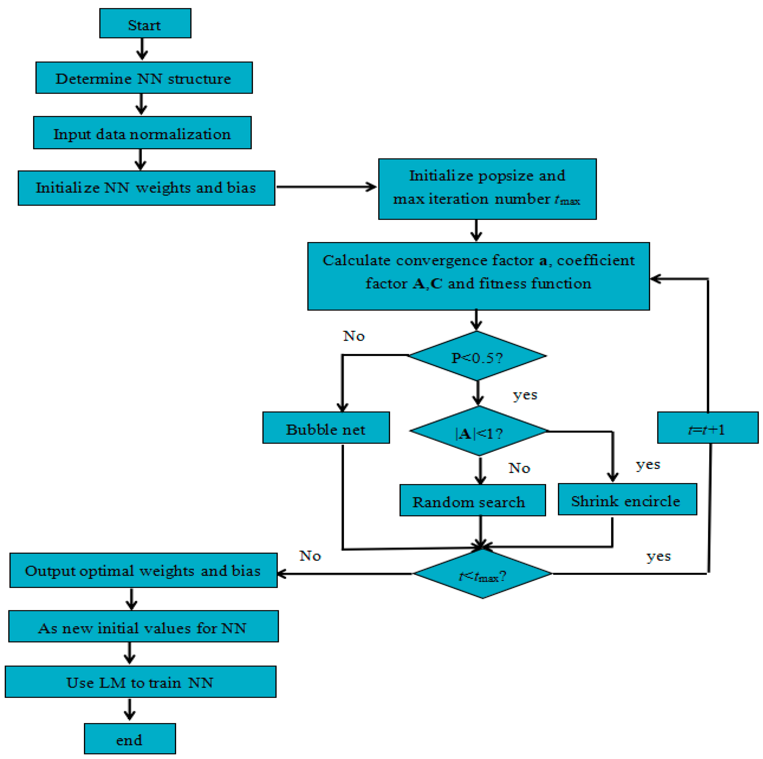
Although the BP neural network trained by the LM algorithm has a good local search ability, it has a strong dependence on the initial connection weights and biases of the network and gets trapped into local minima easily. The WOA aims to search for global optimal solutions in a three-step process: exploration, exploitation, and updating. (1) The exploration phase: through imitating the encircling prey behavior, the position of whales is updated using a predefined equation that encourages exploration and diversification within the search space. (2) The exploitation phase: the algorithm emulates the bubble-net feeding behavior, which aims to locate and exploit promising regions in the search space. (3) Updating phase: through adjusting the positions of whales by considering their current positions, the best solution, and randomization factors, the positions of whales are updated based on the current best solution found so far. This phase aims to balance exploration and exploitation to converge efficiently toward optimal solutions. Through cooperation and information sharing among individuals within the population, the leader position in the WOA combines the global optimal solution and the individual optimal solution, meaning it has the ability to jump out of the local minima and find the global optimal solutions. In addition, the LM algorithm has a better local search ability and can improve the convergence rate of the BP neural network. By combining these two optimization algorithms together, the WOA–LM–BP neural network aims to provide a robust and efficient optimization algorithm for WTC retrieval. The flow chart of the WOA–LM–BP network is shown in Figure 1.
The WOA–LM–BP network starts by determining the network architecture; due to the three-layer network it can approximate any nonlinear problem infinitely. Therefore, the network for retrieval is also a three-layer network with three neurons in the input layer and one neuron in the output layer; that is to say, three calibrated TB are input each time and one predictive retrieved WTC is the output. The neuron number of the hidden layer is 11, the activation function between the input layer and the hidden layer is the hyperbolic tangent sigmoid (tansig), and the activation function between the hidden layer and output layer is a linear function (purelin).
The WOA starts by initializing the popsize of candidates’ solutions and setting the maximum iteration number. During each iteration, referred to as a generation, the WOA assesses the fitness of each solution by computing the objective function value and then utilizes the three strategies to improve the solution. The WOA process continues iterating the three phases until a termination criterion is met, such as reaching the maximum number of iterations or achieving a desired fitness level. The optimal output of WOA is used as the new initial weights and bias for the network, and then the LM algorithm is adopted to train the network until it outputs the optimal local minima.
3. Experimental Data and Processing
3.1. On-Orbit Calibration Experimental Data Processing
The RTM is used to calculate the simulated radiance with known atmospheric conditions, which can be adopted to compare with the actual antenna temperature of the microwave radiometer for calibration or compare with calibrated TB for assessing the biases quantitatively. The inputs of the RTM are atmosphere profile, surface characteristics, radiometer frequency, observation angle, etc.; among them, Numerical Weather Prediction (NWP) models are important sources of information for providing atmospheric profile and surface characteristic data. Therefore, in the scope of this study, the OMB analysis is determined by using the RTM with inputs from the NWP model to calculate the TB,simu regarded as the ground truth [35]. In addition, the RTM adopted in this study is the Fast Microwave Emissivity Model (FASTEM3), which is appropriate for various microwave frequencies with incidence angles less than 60°, and atmospheric absorption model MPM93 [36,37].
ERA-5 is the fifth-generation global atmospheric reanalysis dataset produced by Copernicus Climate Change Service (C3S) at the European Centre for Medium-Range Weather Forecasts (ECMWF) [38]. ERA-5 reanalysis dataset is achieved by assimilation, which combines satellite observations and weather station measurements [39]. This paper adopts an hourly estimation of surface parameters and atmospheric parameters provided by ERA-5 at a horizontal resolution of 31 km and 37 vertical model levels. The input variables for the RTM include the three-dimensional atmospheric parameters, like atmospheric temperature and specific cloud liquid water content, as well as the two-dimensional surface parameters, like wind speed and wind direction. We experiment on a dataset constructed by the CMR current antenna temperatures TA and its along-tracked simulated TB with the time from 15 October 2020 to 24 October 2020, 21 January 2021 to 31 January 2021, 21 April 2021 to 30 April 2021, and from 19 July 2021 to 28 July 2021 (corresponding to cycle 003, cycle 013, cycle 022, and cycle 031 of HY-2C CMR).
Considering the different temporal and spatial resolution of the ERA-5 reanalysis data compared with the CMR observation data, and to reduce the generation time of matched data, we first find out eight adjacent ERA-5 grid points in the period adjacent to the CMR observation points at the hourly scale and then put these data into the RTM to obtain the corresponding TB,simu at each grid point. Subsequently, we apply interpolation on the TB,simu obtained before in the spatial and temporal dimensions, and take the time, latitude, and longitude of the CMR observation point as the criterion to select the along-tracked TB,simu by three linear interpolations.
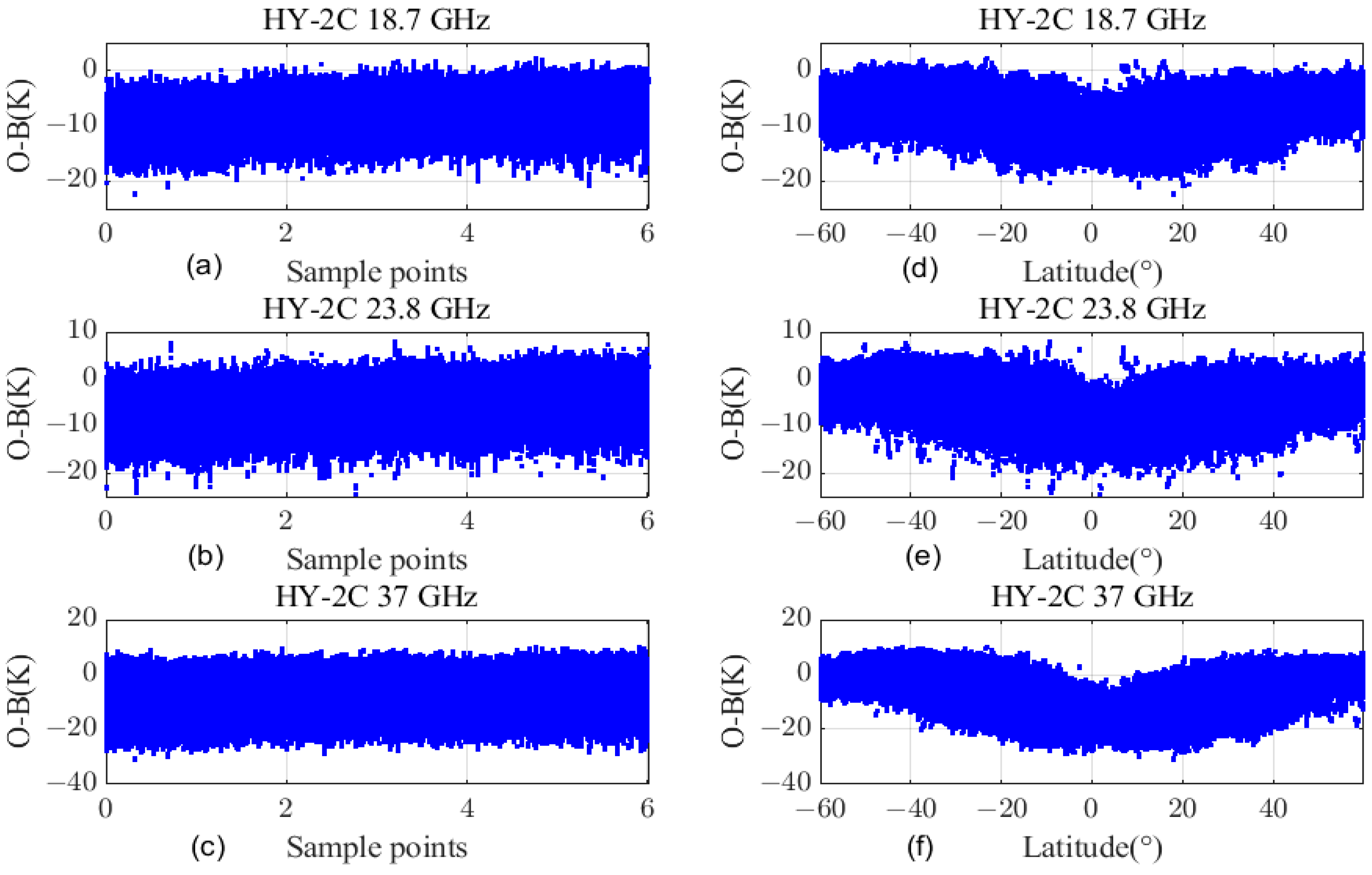
In addition, due to the high temporal and spatial variation of water vapor and cloud liquid water content, and to improve the consistency for comparison, the along-tracked TB,simu need to be filtered: (1) To avoid sea ice contamination, the matched data are limited to the zone between 60°S and 60°N, and the data covered with sea ice within this range are also removed with an ice flag; (2) To reduce the impact of land, coast, and rainy situations, the data classified as land, rain, and offshore distance smaller than 50 km are filtered; (3) Although microwave radiation has the capability to penetrate certain non-precipitating clouds, it cannot effectively penetrate thick precipitation clouds. Additionally, even in penetrable clouds, microwave radiation can still be affected by various particles through absorption, emission, and scattering [40,41]. Therefore, to avoid the uncertainty due to the cloud liquid water, we intend to choose the observations in the clear sky where all cloud data with a liquid water content larger than 0.1 kg/m2 and the standard deviation between adjacent observations greater than 1 K are removed. Figure 2 shows the OMB differences between CMR TA and TB,simu in the whole dataset.
Figure 2a–c shows the OMB differences with time (sample points are arranged in sequence) for each channel. It is evident that the OMB differences vary with the frequency, with the highest magnitude observed at 37.0 GHz and the smallest at 18.7 GHz. The total bias value is within −31~10 K, the total standard deviation is within 3~7 K, and it exhibits no apparent seasonal variation. Figure 2d–f shows the OMB differences with latitude for each channel where the OMB differences vary considerably over latitude. Therefore, an on-orbit calibration effort is required. Two-thirds of the data are randomly selected from the above dataset as the training dataset to perform the calibration algorithm, and the remaining one-third of the data is used as the test dataset (Test Dataset 1) to evaluate the calibrated results.
3.2. Wet Tropospheric Correction Experimental Data Processing
With the global coverage and large quantities of meteorological reanalysis, the NWP data also have been widely used to compute the model-derived WTC. In this paper, we use the profile data from ERA-5 to calculate the model-derived WTC (hereafter, WTCmodel). At each grid point, the ERA-5 profile data include 16 atmospheric parameters on 37 pressure levels, from the surface at 1000 hPa to the altitude of around 45~50 km (1 hPa). Generally, the WTC includes the contribution from two parts: water vapor-induced WTC and cloud liquid water-induced WTC. Compared with water vapor-induced WTC, the cloud liquid water-induced WTC is only a very small component (less than 1 mm), which is 1~2 orders of magnitude smaller than the effect of water vapor under non-raining conditions [42,43,44]. In the scope of this study, the WTC refers to the water vapor-induced WTC, and the WTC computation from these 3-D atmospheric variables is performed through the numerical integration of specific humidity and temperature along the vertical profiles, and the expression is written as [45]:
where PTOA and Psurf are the top of the atmosphere and the surface pressure given in hPa. Due to the fact that the specific humidity approaches zeros above 200 hPa (around 12 km), making the corresponding WTC close to zero, for the computation efficiency we make Psurf be 1000 hPa and PTOA be 200 hPa. q represents the specific humidity in kg/kg, which means the mass of water vapour per kilogram of moist air. T is the temperature in Kelvin, φ is the latitude, and WTCmodel is in meter.
The time of the model-derived WTC used to compare is the same as the time mentioned in Section 3.1 (cycle 003/013/022/031 of HY-2C). Since the model-derived WTC cannot guarantee sufficient accuracy in rainy situations, the along-tracked points selected are all from ocean clear sky field, where the cloud liquid water content is below 1 mm, the latitude range is between 60°S and 60°N, and the observation points are away from the coastline at a distance greater than 50 km, and without the ice coverage. Similar to the calculations of the along-tracked simulated TB,simu, we first calculate the model-derived WTC of eight adjacent grid points and then apply three linear interpolations based on the time and geographic location information of the CMR observation points. In total, there are 1,561,324 geophysical situations in the final database, ensuring a good distribution in time and geography. Two-thirds of the data are randomly selected as the training dataset to perform the retrieval algorithm, and the other third of the data is used as the test dataset to evaluate the retrieval results.
4. Results
4.1. On-Orbit Calibration Results and Analysis
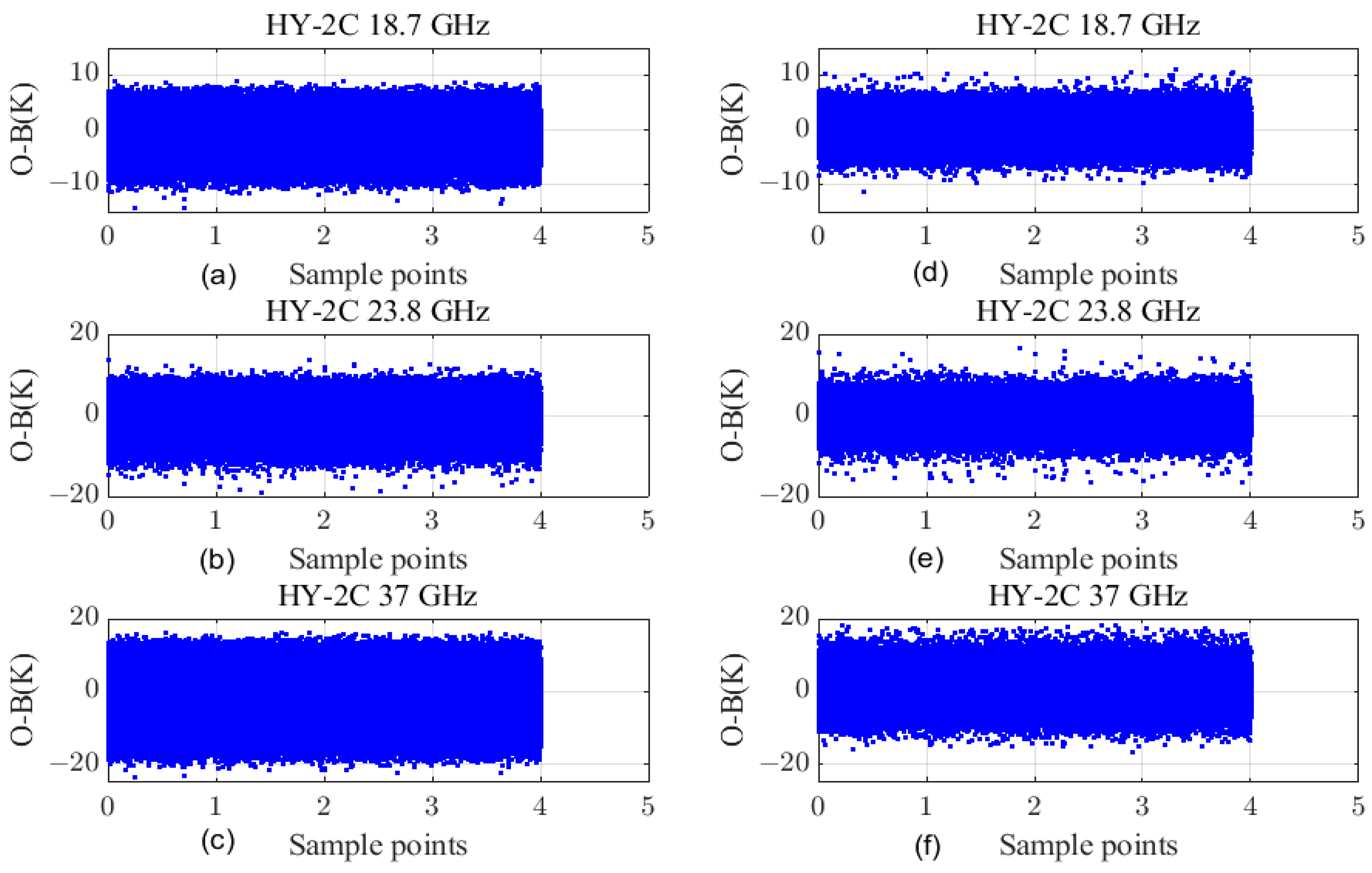
Section 2.1 and Section 2.2 present two calibrated methods: the APC method and the neural network; this section assesses which performs well. The performance of the calibrated TB is evaluated with the TB,simu, taking the results of the training dataset for examples. Figure 3 illustrates the OMB difference of CMR for each channel over time, based on the APC method (left panel) and based on the neural network (right panel). Notably, after calibration the bias between the calibrated TB and the TB,simu is obviously removed; in particular, the neural network exhibits significant improvements both in mean deviation and standard deviation of the OMB difference for all three channels when compared to the APC method.
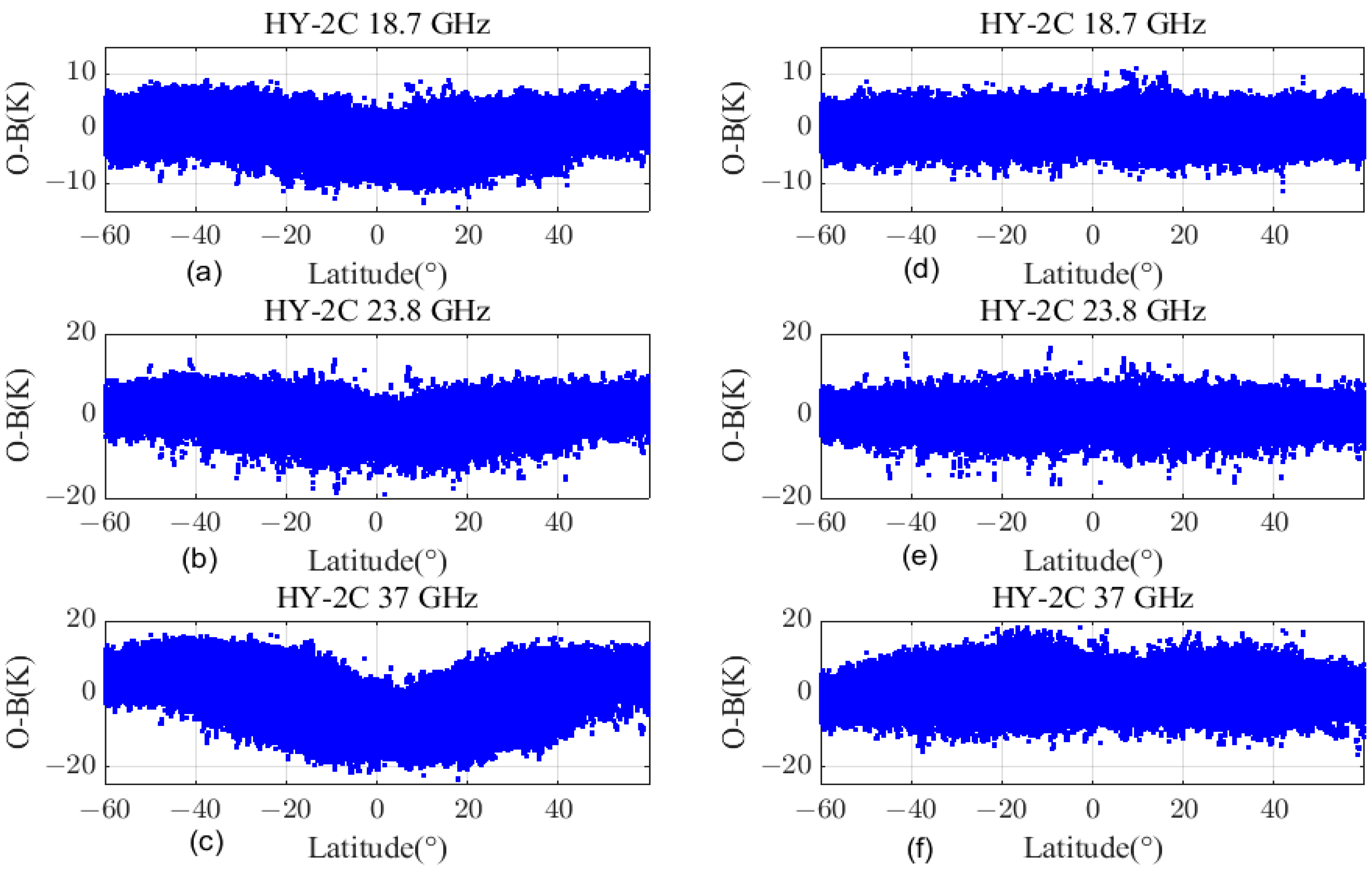
As depicted in Figure 4, it displays the OMB difference of CMR for each channel over latitude, based on the APC approach (left panel) and based on the neural network (right panel). Remarkably, the neural network method can effectively reduce the OMB difference fluctuation with latitude for the three channels.
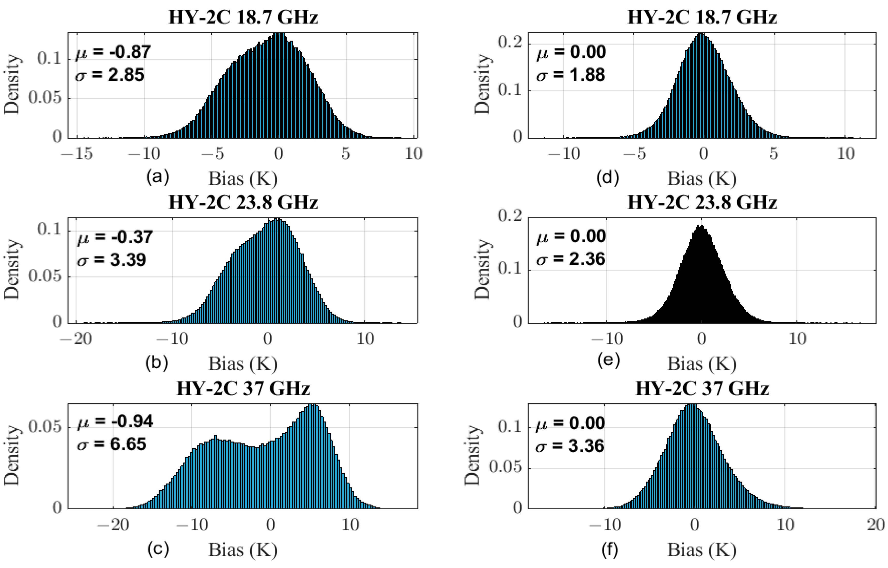
The OMB difference histograms (normalized with the total numbers of the training dataset) of CMR in each channel are given in Figure 5, which can be approximately considered as the probability density distribution of the OMB differences for the APC method (Figure 5a–c) and the neural network (Figure 5d–f). It can be seen that there are clear distinctions between the two methods. For instance, although the OMB differences based on the APC method are all close to the normal distribution, they are a combination of at least two distinct states, especially for the 37 GHz channel, where two obvious peaks are observed. These peaks can be attributed to the lower measurement for the high-temperature targets. The OMB difference based on the neural network is normally distributed with a total bias equal to zeros, which not only removes the inconsistency between the TB,simu and the calibrated TB but also demonstrates the validity of this method.
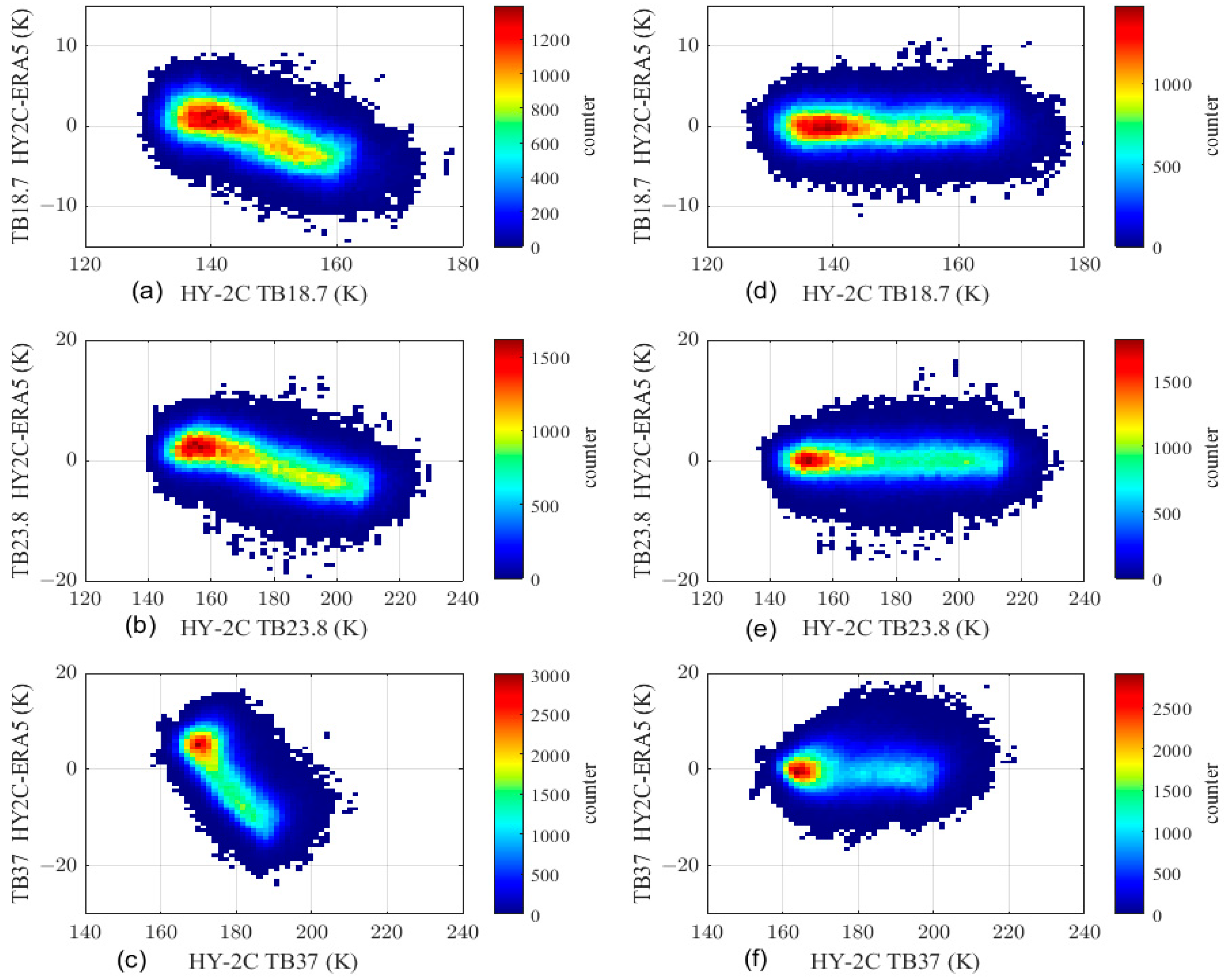
Figure 6 illustrates the OMB differences with respect to the calibrated TB for the same dataset. The color represents the number of points displayed in the colorbar, where the warm color denotes more points and the cold color for fewer points. In the left panels, we observe that at low TBs, a positive bias changes into a negative bias when moving to high values of TB, while this phenomenon disappears when utilizing the neural network method, indicating that it can provide a more consistent agreement with the TB,simu values.
For further evaluating the performance and reliability of the two methods, the main statistics characteristics, such as the mean deviation (MD), standard deviation (STD), root-mean-square error (RMSE), and correlation coefficient, are calculated for the training dataset and test dataset, respectively, and they are summarized in Table 1. For the calibration results, the optimal algorithm is the one which can minimize the difference between the TB,simu and the calibrated TB both in training and test datasets. The mean deviation for each CMR channel on the training dataset with the APC method is −0.87 K, −0.37 K, and −0.94 K, while with the neural network, the mean deviation is reduced to 0 K. Compared with the APC method, the calibrated TB based on the neural network method has a smaller standard deviation and RMSE value, which means a more enhanced agreement with the simulated ones. The statistical results of the test dataset (Test Dataset 1) are similar to those in the training dataset, and to further check the robustness and reliability of the CMR-calibrated TB, we perform another comparison on a dataset (Test Dataset 2) in which cloud liquid water content is within the range of 0~0.1 kg/m2 and the filter criteria of standard deviation smaller than 1 K can be discarded. The calibrated results evaluation on the Test Dataset 2 also confirms that the neural network works well.
4.2. WTC Results and Analysis
Section 2.3 presents a WOA–LM–BP network for retrieving WTC. For investigating the performance of the network, two different methods have been adopted to comprehensively assess the retrieved WTC of CMR: (1) directly compare the WTC difference from the along-tracked model-derived WTC; (2) directly compare the WTC difference from Jason-3 AMR-2 at crossover points.
4.2.1. Assessment with the Model-Derived WTC
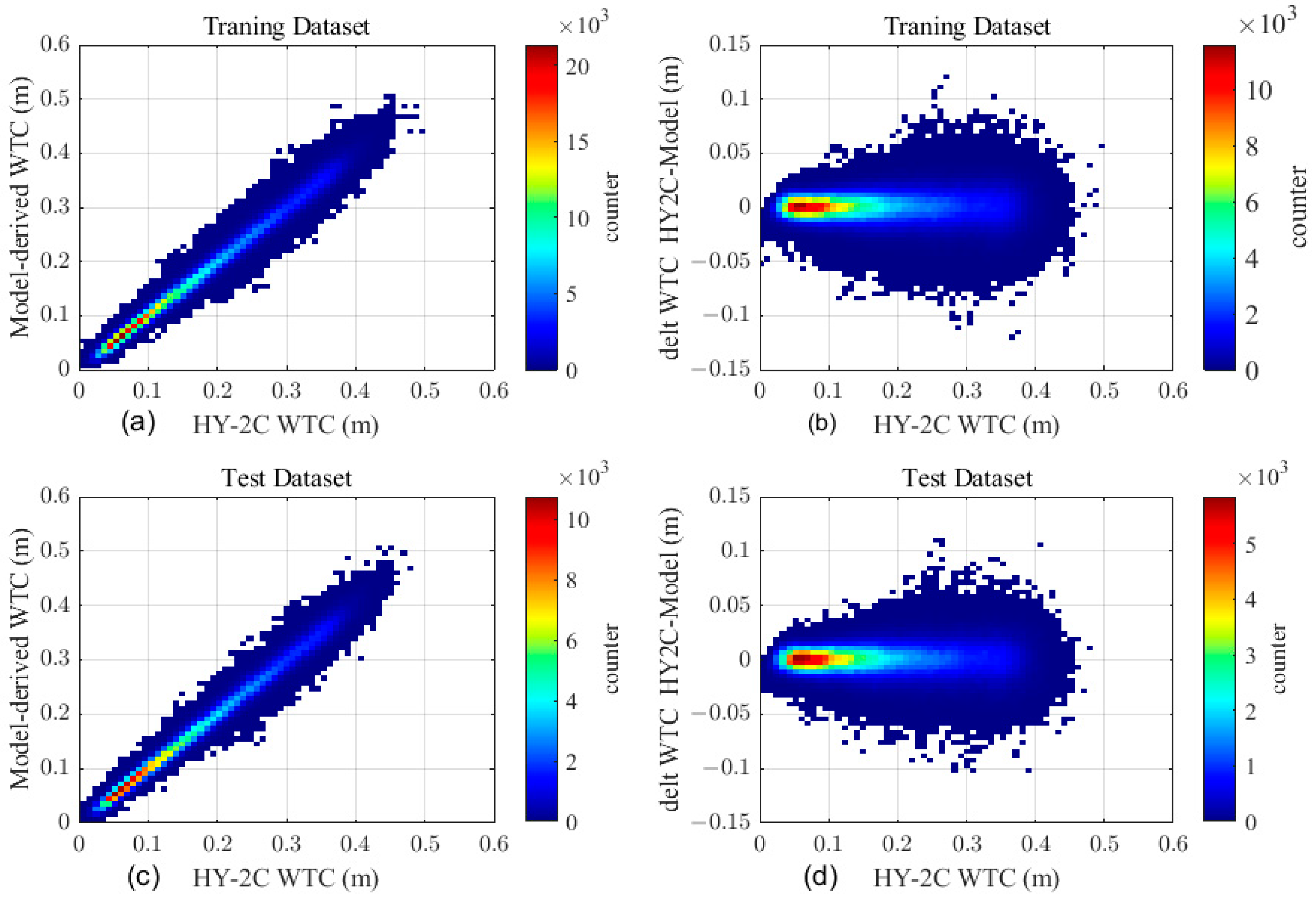
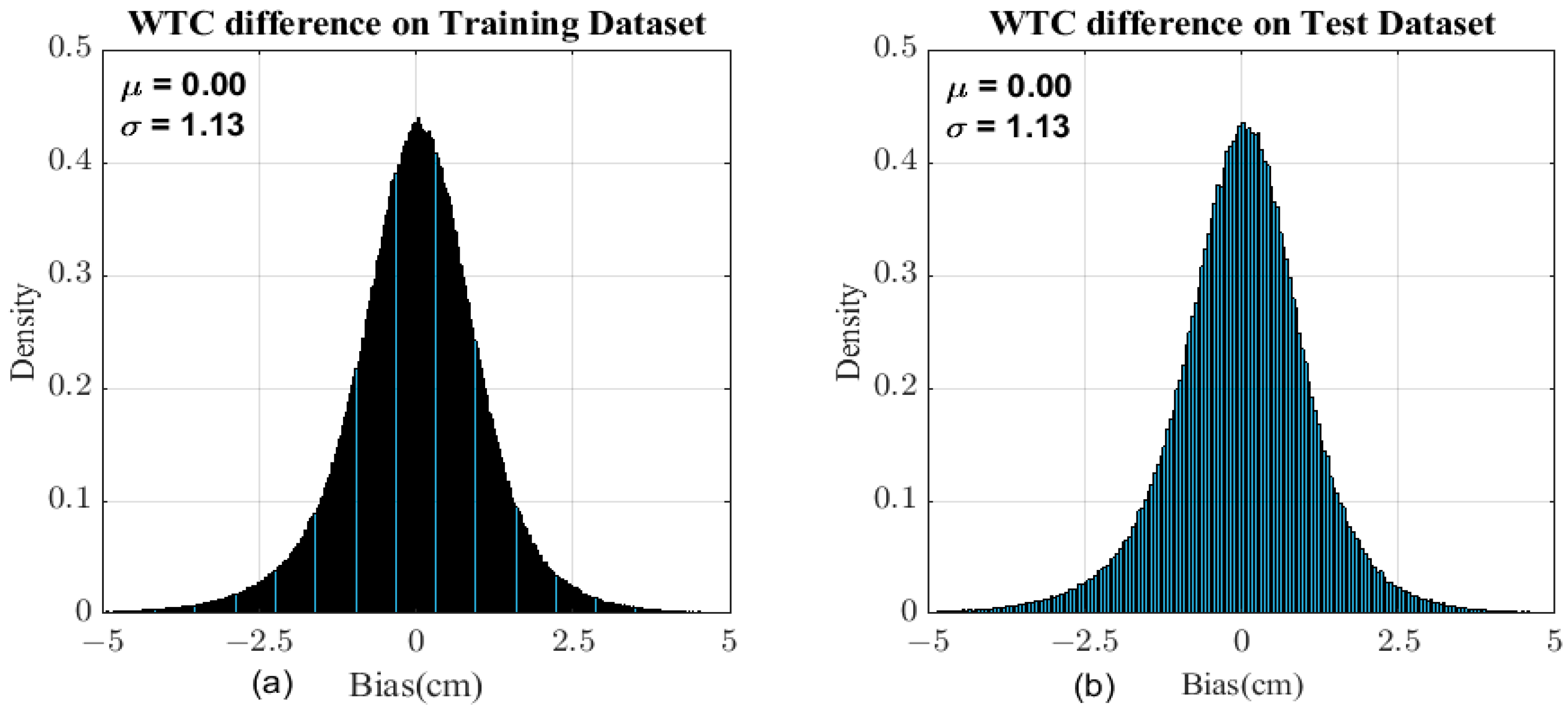
The performance of the retrieved WTC of HY-2C is firstly evaluated with the model-derived WTC with its global coverage to perform a rapid check globally. The left panels of Figure 7 are scatter diagrams of HY-2C WTC with respect to the model-derived WTC for the training dataset (top) and the test dataset (bottom), and the right panels are scatter diagrams of HY-2C WTC with respect to the WTC differences between HY-2C and model-derived WTC. Figure 8 shows the WTC difference histogram of the training dataset and test dataset, which approximate the normal distribution with a total bias close to zero. Table 2 presents the statistical characteristics, except the main statistics characteristics mentioned in Section 4.1. Another parameter, the coefficient of determination (R2), is added to quantify the agreement degree between the HY-2C WTC and the model-derived one. The value of R2 is [0, 1], and a larger value of R2 indicates a better performance of agreement.
Taking the test dataset for illustration, the mean value of the WTC difference is 0.0 cm with a 1.13 cm root-mean-square error. The WTC of HY-2C matches the model-derived WTC well, with the correlation efficient and R2 almost equal to 0.99. All the statistical characteristics demonstrate a good agreement between the HY-2C WTC and the model-derived one, which shows the effectiveness of the retrieval method.
4.2.2. Assessment with the Jason-3 AMR-2 WTC
To prove the reliability of the retrieval results, another independent data source is adopted to examine the retrieval method. We use the SNOs approach to assess the retrieved WTC, where the Jason-3 AMR-2 is chosen as the reference for its high accuracy measurements [46]. Jason-3 is a follow-on satellite of OSTM/Jason-2, and its objective is to provide continuous observation of global ocean circulation and SSH. The orbital altitude of Jason-3 is 1336 km with an inclination of 66°, the revisit period is approximately 10 days with 254 passes, and the latitude range spans from 66.15°S to 66.15°N. The time of Jason-3 GDR-F data is the same as the CMR (cycle 001-cycle 041, from 1 October 2020 to 31 October 2021), and these data are available from the Archiving, Validation, and Interpretation of Satellite Oceanographic (AVISO) data center.
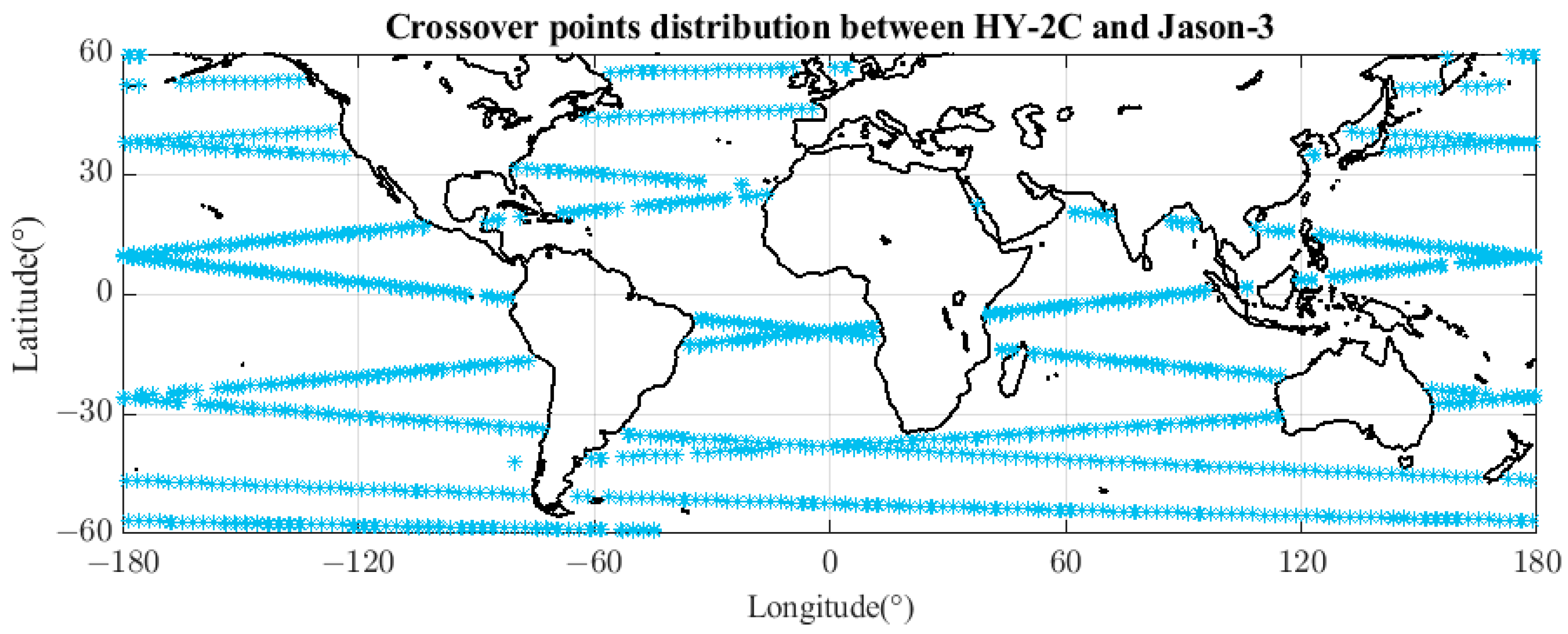
To obtain high-quality comparison results, before performing the SNOs the crossover points between the HY-2C and Jason-3 have to apply quality control by status flags and threshold screening: (1) Considering the global coverage of CMR and Jason-3, the latitude range is between 60°S and 60°N; (2) Using the “surface_type”, “rain_flag”, and “ice_flag” to screen the open ocean areas without rain and ice coverage; (3) To reduce the land contamination, crossover points at a distance less than 50 km are screened out; (4) The crossover points within the time interval of 30 min and the distance interval of 30 km of HY-2C and Jason-3 are selected. The final number of crossover points during one year is 14,518, which ensures a global distribution in time and geography. Figure 9 shows the global distribution of crossover points.
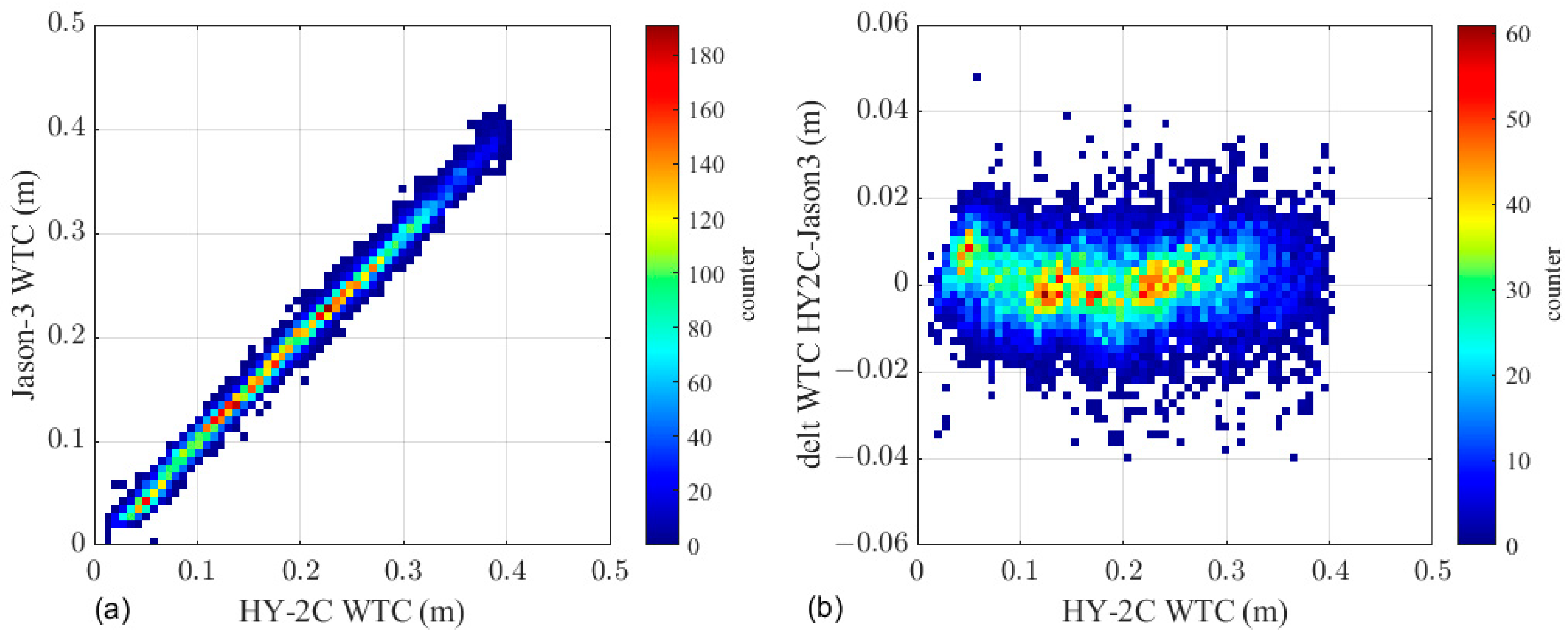
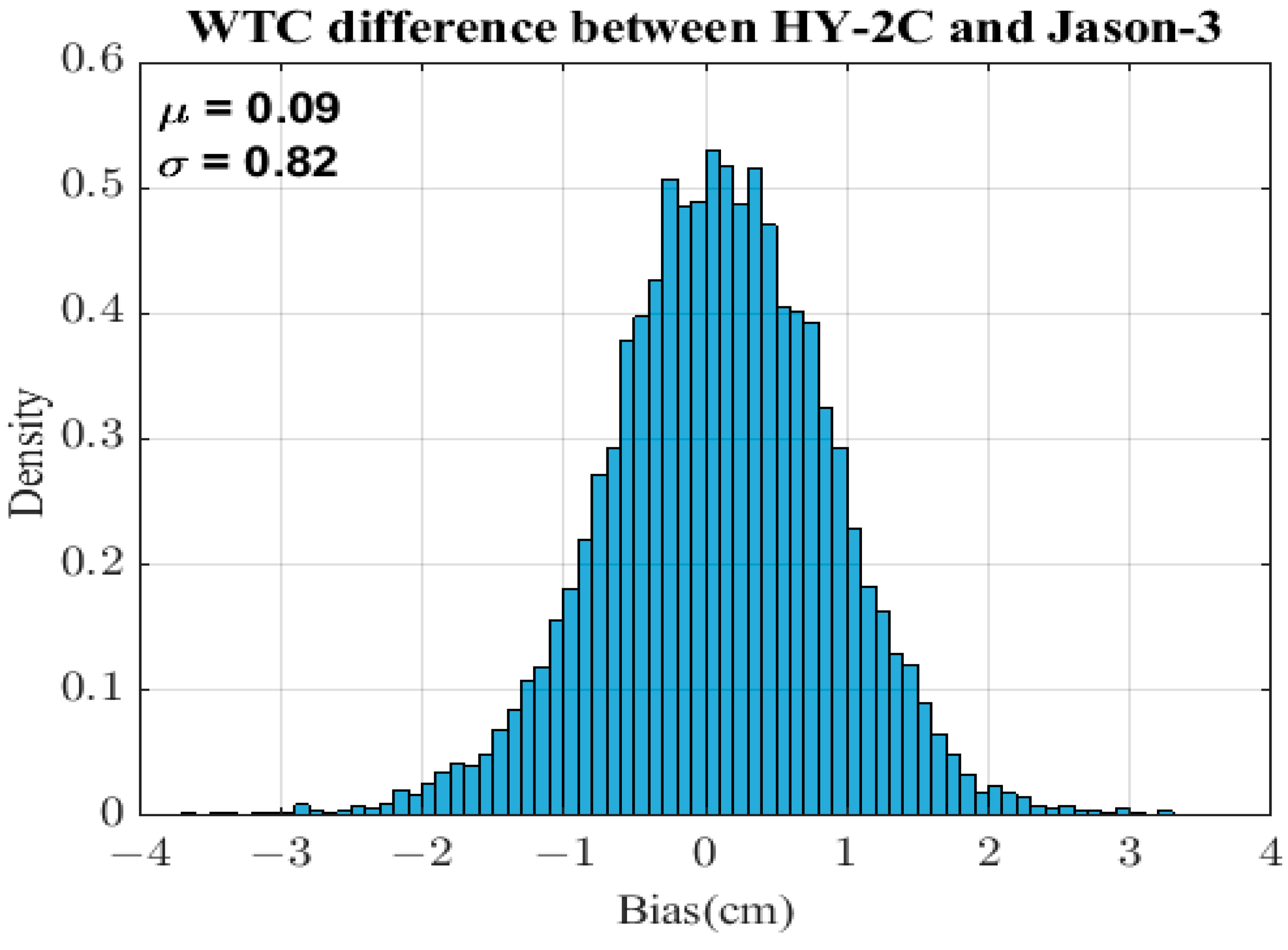
The left panel of Figure 10 is the scatter diagram of HY-2C WTC with respect to Jason-3 WTC for HY-2C cycle 001-cycle 041 (in m), and the right panel is the scatter diagram of HY-2C WTC with respect to the WTC differences between HY-2C and Jason-3. Figure 11 presents the WTC difference histogram of the crossover points, and the statistical characteristics are summarized in Table 2.
The mean deviation and the RMS between the HY-2C WTC and the Jason-3 WTC are 0.09 cm and 0.82 cm, respectively, and the correlation coefficient and R2 are 0.9959 and 0.9918, respectively. They all demonstrate that the HY-2C WTC has a good agreement with Jason-3.
5. Conclusions
The calibrated brightness temperatures of microwave radiometers can be used to retrieve the WTC; with the HY-2C CMR operating in its designed orbit for more than 2 years, this study focuses on the on-orbit calibration algorithm and the WTC retrieval algorithm of HY-2C CMR.
We first present the APC method and the neural method to calibrate the antenna temperature, and then use the OMB method to assess the two methods, which compares the calibrated brightness temperatures to the simulated brightness temperatures calculated by the RTM using input from NWP. Taking the Test Dataset 1 for illustration, the comparison results show that compared with the APC method, the mean deviation of the calibrated brightness temperature derived by the neural network is clearly reduced by about 0.86, 0.34, and 0.90 K in the three channels, respectively; the RMSE are reduced by about 1.10, 1.06, and 3.34 K, respectively. After broadening the along-tracked observations filter criterion, the calibrated brightness temperature derived by the neural network still has better agreement with the simulated ones than that derived from the APC method, which demonstrates the effectiveness of the neural network calibration method.
The primary purpose of using the WOA–LM–BP model is to improve the retrieval accuracy for HY-2C; the WOA is used to avoid falling into local minima and find the optimal initial network parameters, and then the LM algorithm is used to find the optimal local minima under the obtained network parameter, so as to improve the accuracy of the retrieved WTC. The results of the retrieved HY-2C WTC are compared with the model-derived WTC on the test dataset and the crossover points from Jason-3 over one year; all the statistical characteristics indicate that the retrieved WTC of HY-2C has a good performance, satisfying the mission requirements well.
Author Contributions
Methodology, X.Z. and J.Z.; Software, X.Z.; Validation, X.Z. and M.J.; Writing—original draft, X.Z.; Writing—review and editing, D.Z. All authors have read and agreed to the published version of the manuscript.
Funding
This research received no external funding.
Data Availability Statement
The data are not publicly available due to privacy.
Acknowledgments
The authors are grateful to the Archiving, Validation, and Interpretation of Satellite Oceanographic Data (AVISO) for providing Jason-3 Geophysical Data Records products, to the National Satellite Ocean Application Service (NSOAS), State Oceanic Administration, China for providing the HY-2C Interim Geophysical Data Records products, to the European Centre for Medium-Range Weather Forecasts for providing the fifth version reanalysis products of surface and profile data, and to the National Centers for Environmental Prediction for providing the reanalysis data products.
Conflicts of Interest
The authors declare no conflict of interest.
References
- Tian, J.; Shi, J. A High-Accuracy and Fast Retrieval Method of Atmospheric Parameters Based on Genetic-BP. IEEE Access 2022, 10, 19458–19468. [Google Scholar] [CrossRef]
- Xu, X.-Y.; Xu, K.; Shen, H.; Liu, Y.-L.; Liu, H.-G. Sea Surface Height and Significant Wave Height Calibration Methodology by a GNSS Buoy Campaign for HY-2A Altimeter. IEEE J. Sel. Top. Appl. Earth Obs. Remote Sens. 2016, 9, 5252–5261. [Google Scholar] [CrossRef]
- Chen, C.; Zhu, J.; Ma, C.; Lin, M.; Yan, L.; Huang, X.; Zhai, W.; Mu, B.; Jia, Y. Preliminary calibration results of the HY-2B altimeter’s SSH at China’s Wanshan calibration site. Acta Oceanol. Sin. 2021, 40, 129–140. [Google Scholar] [CrossRef]
- Zheng, X.; Zhang, D.; Zhao, J.; Jiang, M. Brightness Temperature and Wet Tropospheric Correction of HY-2C Calibration Microwave Radiometer Using Model-Derived Wet Troposphere Path Delay from ECMWF. Remote Sens. 2023, 15, 1318. [Google Scholar] [CrossRef]
- Bao, L.; Gao, P.; Peng, H.; Jia, Y.; Shum, C.K.; Lin, M.; Guo, Q. First accuracy assessment of the HY-2A altimeter sea surface height observations: Cross-calibration results. Adv. Space Res. 2015, 55, 90–105. [Google Scholar] [CrossRef]
- Zheng, G.; Yang, J.; Ren, L.; Zhou, W.; Huang, L. The preliminary cross-calibration of the HY-2A calibration microwave radiometer with the Jason-1/2 microwave radiometers. Int. J. Remote Sens. 2014, 35, 4515–4531. [Google Scholar] [CrossRef]
- Wang, Z.; Xiao, Y.; Wang, K.; Zhang, S. Recalibration MWHTS’historical data onboard FY3C based on the response characteristics of microwave radiometer. Natl. Remote Sens. Bull. 2022, 14, 1–11. [Google Scholar] [CrossRef]
- Zhang, C.; Qi, C.; Yang, T.; Gu, M.; Zhang, P.; Lee, L.; Xie, M.; Hu, X. Evaluation of FY-3E/HIRAS-II Radiometric Calibration Accuracy Based on OMB Analysis. Remote Sens. 2022, 14, 3222. [Google Scholar] [CrossRef]
- Brown, S.; Ruf, C.; Keihm, S.; Kitiyakara, A. Jason Microwave Radiometer Performance and On-Orbit Calibration. Mar. Geodesy 2004, 27, 199–220. [Google Scholar] [CrossRef]
- Frery, M.-L.; Siméon, M.; Goldstein, C.; Féménias, P.; Borde, F.; Houpert, A.; Garcia, A.O. Sentinel-3 Microwave Radiometers: Instrument Description, Calibration and Geophysical Products Performances. Remote Sens. 2020, 12, 2590. [Google Scholar] [CrossRef]
- Picard, B.; Frery, M.-L.; Obligis, E.; Eymard, L.; Steunou, N.; Picot, N. SARAL/AltiKa Wet Tropospheric Correction: In-Flight Calibration, Retrieval Strategies and Performances. Mar. Geodesy 2015, 38, 277–296. [Google Scholar] [CrossRef] [Green Version]
- Ruf, C.S.; Keihm, S.J.; Subramanya, B.; Janssen, M.A. TOPEX/POSEIDON microwave radiometer performance and in-flight calibration. J. Geophys. Res. Atmos. 1994, 99, 24915. [Google Scholar] [CrossRef]
- Eymard, L.; Tabary, L.; Gerard, E.; Boukabara, S.; Le Cornec, A. The microwave radiometer aboard ERS-1. II. Validation of the geophysical products. IEEE Trans. Geosci. Remote Sens. 1996, 34, 291–303. [Google Scholar] [CrossRef]
- Fernandes, M.J.; Lázaro, C.; Ablain, M.; Pires, N. Improved wet path delays for all ESA and reference altimetric missions. Remote Sens. Environ. 2015, 169, 50–74. [Google Scholar] [CrossRef] [Green Version]
- Obligis, E.; Eymard, L.; Tran, N.; Labroue, S.; Femenias, P. First Three Years of the Microwave Radiometer aboard Envisat: In-Flight Calibration, Processing, and Validation of the Geophysical Products. J. Atmos. Ocean. Technol. 2006, 23, 802–814. [Google Scholar] [CrossRef]
- Vieira, T.; Fernandes, M.J.; Lázaro, C. An enhanced retrieval of the wet tropospheric correction for Sentinel-3 using dynamic inputs from ERA5. J. Geod. 2022, 96, 28. [Google Scholar] [CrossRef]
- Chakraborty, R.; Maitra, A. Retrieval of atmospheric properties with radiometric measurements using neural network. Atmos. Res. 2016, 181, 124–132. [Google Scholar] [CrossRef]
- Dorigo, M.; Birattari, M. Ant Colony Optimization. In Encyclopedia of Machine Learning and Data Mining; Springer: Berlin/Heidelberg, Germany, 2017; pp. 56–59. [Google Scholar] [CrossRef]
- Kenmedy, J.; Eberhart, R. Particle swarm optimization. In Proceedings of the IEEE International Conference on Neural Networks, Perth, Australia, 27 November–1 December 1995; IEEE: Piscataway, NJ, USA, 1995; pp. 1942–1948. [Google Scholar]
- Mirjalili, S.; Lewis, A. The Whale Optimization Algorithm. Adv. Eng. Softw. 2016, 95, 51–67. [Google Scholar] [CrossRef]
- Hasanien, H.M. Performance improvement of photovoltaic power systems using an optimal control strategy based on whale optimization algorithm. Electr. Power Syst. Res. 2018, 157, 168–176. [Google Scholar] [CrossRef]
- Feng, W.; Deng, B. Global convergence analysis and research on parameter selection of whale optimization algorithm. Control Theory Appl. 2021, 38, 641–651. (In Chinese) [Google Scholar]
- Brown, S.T.; Desai, S.; Lu, W.; Tanner, A. On the Long-Term Stability of Microwave Radiometers Using Noise Diodes for Calibration. IEEE Trans. Geosci. Remote Sens. 2007, 45, 1908–1920. [Google Scholar] [CrossRef]
- Crews, A.; Blackwell, B.; Leslie, V.; Cahoy, K.; DiLiberto, M.; Milstein, A.; Osaretin, I.; Grant, M. Calibration and validation of small satellite passive microwave radiometers: MicroMAS-2A and TROPICS. In Proceedings of the Volume 10788, Active and Passive Microwave Remote Sensing for Environmental Monitoring II; SPIE-International Society for Optics and Photonics: Bellingham, WA, USA, 2018; Volume 35. [Google Scholar] [CrossRef]
- Wang, Z.; Zhang, D.; Li, Y.; Zhao, J. Prelaunch calibration and primary results from in-orbit calibration of the atmospheric correction microwave radiometer (ACMR) on the HY-2A satellite of China. Int. J. Remote Sens. 2014, 35, 4496–4514. [Google Scholar] [CrossRef]
- Obligis, E.; Eymard, L.; Tran, N. A New Sidelobe Correction Algorithm for Microwave Radiometers: Application to the Envisat Instrument. IEEE Trans. Geosci. Remote Sens. 2007, 45, 602–612. [Google Scholar] [CrossRef]
- Available online: https://www.remss.com/measurements/brightness-temperature (accessed on 6 June 2023).
- Bernard, R.; Le Cornec, A.; Eymard, L.; Tabary, L. The microwave radiometer aboard ERS-1.1. Characteristics and performances. IEEE Trans. Geosci. Remote Sens. 1993, 31, 1186–1198. [Google Scholar] [CrossRef]
- Mo, T. AMSU-A antenna pattern corrections. IEEE Trans. Geosci. Remote Sens. 1999, 37, 103–112. [Google Scholar] [CrossRef]
- Janssen, M.; Ruf, C.; Keihm, S. TOPEX/Poseidon Microwave Radiometer (TMR). II. Antenna pattern correction and brightness temperature algorithm. IEEE Trans. Geosci. Remote Sens. 1995, 33, 138–146. [Google Scholar] [CrossRef]
- Okuyama, A.; Imaoka, K. Intercalibration of Advanced Microwave Scanning Radiometer-2 (AMSR2) Brightness Temperature. IEEE Trans. Geosci. Remote Sens. 2015, 53, 4568–4577. [Google Scholar] [CrossRef]
- Obligis, E.; Tran, N.; Eymard, L. An Assessment of Jason-1 Microwave Radiometer Measurements and Products. Mar. Geod. 2004, 27, 255–277. [Google Scholar] [CrossRef]
- Zhang, Z.; Dong, X.; Liu, L.; He, J. Retrieval of Barometric Pressure from Satellite Passive Microwave Observations over the Oceans. J. Geophys. Res. Oceans 2018, 123, 4360–4372. [Google Scholar] [CrossRef]
- Feng, M.; Ai, W.; Lu, W.; Shan, C.; Ma, S.; Chen, G. Sea surface temperature retrieval based on simulated microwave polarimetric measurements of a one-dimensional synthetic aperture microwave radiometer. Acta Oceanol. Sin. 2021, 40, 122–133. [Google Scholar] [CrossRef]
- Crews, A. Calibration and Validation for CubeSat Microwave Radiometers; Massachusetts Institute of Technology: Cambridge, MA, USA, 2019. [Google Scholar]
- Wang, Z.; Zhang, D. Simulation on Retrieving of Atmospheric Wet Path Delay by Microwave Radiometer on HY-2 Satellite. In Proceedings of the 2008 China-Japan Joint Microwave Conference, Shanghai, China, 10–12 September 2008; pp. 665–668. [Google Scholar] [CrossRef]
- Liebe, H.J.; Hufford, G.A.; Cotton, M.G. Propagation modeling of moist air and suspended water/ice particles at frequencies below 1000 GHz. In Proceedings of the AGARD 52nd Specialists Meeting of the Electromagnetic Wave Propagation Panel, Palma de Mallorca, Spain, 17–21 May 1993; pp. 3.1–3.10. [Google Scholar]
- Available online: https://www.ecmwf.int/en/forecasts/dataset/ecmwf-reanalysis-v5 (accessed on 6 June 2023).
- Xi, X.; Gentine, P.; Zhuang, Q.; Kim, S. Evaluating the effects of precipitation and evapotranspiration on soil moisture variability. Purdue Univ. Res. Repos. 2022. [Google Scholar] [CrossRef]
- Greenwald, T.J.; Bennartz, R.; Lebsock, M.; Teixeira, J. An Uncertainty Data Set for Passive Microwave Satellite Observations of Warm Cloud Liquid Water Path. J. Geophys. Res. Atmos. 2018, 123, 3668–3687. [Google Scholar] [CrossRef] [PubMed]
- Bennartz, R.; Watts, P.; Meirink, J.F.; Roebeling, R. Rainwater path in warm clouds derived from combined visible/near-infrared and microwave satellite observations. J. Geophys. Res. Atmos. 2010, 115. [Google Scholar] [CrossRef]
- Keihm, S.; Janssen, M.; Ruf, C. TOPEX/Poseidon microwave radiometer (TMR). III. Wet troposphere range correction algorithm and pre-launch error budget. IEEE Trans. Geosci. Remote Sens. 1995, 33, 147–161. [Google Scholar] [CrossRef]
- Zheng, G.; Yang, J.; Ren, L. Retrieval Models of Water Vapor and Wet Tropospheric Path Delay for the HY-2A Calibration Microwave Radiometer. J. Atmos. Ocean. Technol. 2014, 31, 1516–1528. [Google Scholar] [CrossRef]
- Fernandes, M.J.; Lázaro, C. Independent Assessment of Sentinel-3A Wet Tropospheric Correction over the Open and Coastal Ocean. Remote Sens. 2018, 10, 484. [Google Scholar] [CrossRef] [Green Version]
- Vieira, T.; Fernandes, M.J.; Lázaro, C. Modelling the Altitude Dependence of the Wet Path Delay for Coastal Altimetry Using 3-D Fields from ERA5. Remote Sens. 2019, 11, 2973. [Google Scholar] [CrossRef] [Green Version]
- Jia, Y.; Yang, J.; Lin, M.; Zhang, Y.; Ma, C.; Fan, C. Global Assessments of the HY-2B Measurements and Cross-Calibrations with Jason-3. Remote Sens. 2020, 12, 2470. [Google Scholar] [CrossRef]
Figure 1.
Flow chart of the WOA–LM –BP model.

Figure 2.
Diagram of OMB differences before calibration of CMR for each channel. (a–c): over time; (d–f): over latitude.
Figure 2.
Diagram of OMB differences before calibration of CMR for each channel. (a–c): over time; (d–f): over latitude.

Figure 3.
Diagram of OMB differences of CMR for each channel over time. (a–c): based on the APC method; (d–f): based on the neural network.
Figure 3.
Diagram of OMB differences of CMR for each channel over time. (a–c): based on the APC method; (d–f): based on the neural network.

Figure 4.
Diagram of OMB differences of CMR for each channel over latitude. (a–c): based on the APC method; (d–f): based on the neural network.
Figure 4.
Diagram of OMB differences of CMR for each channel over latitude. (a–c): based on the APC method; (d–f): based on the neural network.

Figure 5.
Histogram of OMB differences of CMR for each channel on training dataset. (a–c): based on the APC method; (d–f): based on the neural network.
Figure 5.
Histogram of OMB differences of CMR for each channel on training dataset. (a–c): based on the APC method; (d–f): based on the neural network.

Figure 6.
Diagram of OMB differences of HY-2C for each channel with respect to the calibrated TB on training dataset. (a–c): based on the APC method; (d–f): based on the neural network (x representing the calibrated TB and y the simulated one). Color denotes the number of points displayed in the color bar.

Figure 7.
(a): HY-2C WTC versus model-derived WTC in training dataset; (b) HY-2C WTC versus WTC difference between HY-2C and model-derived WTC in training dataset; (c): HY-2C WTC versus model-derived WTC in test dataset; (d) HY-2C WTC versus WTC difference between HY-2C and model-derived WTC in test dataset; Color indicates the number of points displayed in the colorbar.

Figure 8.
Histogram of WTC differences between HY-2C and model-derived WTC. (a): on training dataset; (b): on test dataset.
Figure 8.
Histogram of WTC differences between HY-2C and model-derived WTC. (a): on training dataset; (b): on test dataset.

Figure 9.
Crossover points distribution between HY-2C and Jason-3 over one year.

Figure 10.
(a): HY-2C WTC versus Jason-3 WTC. (b) HY-2C WTC versus WTC difference between HY-2C and Jason-3.
Figure 10.
(a): HY-2C WTC versus Jason-3 WTC. (b) HY-2C WTC versus WTC difference between HY-2C and Jason-3.

Figure 11.
Histogram of WTC differences between CMR and Jason-3.


Table 1.
Statistical characteristics for the comparison between the calibrated TB of CMR and the TB,simu.
Table 1.
Statistical characteristics for the comparison between the calibrated TB of CMR and the TB,simu.
| Dataset | Channel (GHz) | Method | MD (K) | STD (K) | RMSE (K) | Corr |
|---|---|---|---|---|---|---|
| Training Dataset | 18.7 | APC | −0.87 | 2.85 | 2.98 | 0.98 |
| NN | 0.00 | 1.88 | 1.88 | 0.98 | ||
| 23.8 | APC | −0.37 | 3.39 | 3.41 | 0.99 | |
| NN | 0.00 | 2.36 | 2.36 | 0.99 | ||
| 37 | APC | −0.94 | 6.65 | 6.72 | 0.94 | |
| NN | 0.00 | 3.36 | 3.36 | 0.97 | ||
| Test Dataset 1 | 18.7 | APC | −0.86 | 2.86 | 2.98 | 0.98 |
| NN | 0.00 | 1.88 | 1.88 | 0.98 | ||
| 23.8 | APC | −0.35 | 3.39 | 3.41 | 0.99 | |
| NN | 0.01 | 2.35 | 2.35 | 0.99 | ||
| 37 | APC | −0.91 | 6.65 | 6.71 | 0.94 | |
| NN | 0.01 | 3.37 | 3.37 | 0.97 | ||
| Test Dataset 2 | 18.7 | APC | −0.77 | 2.94 | 3.04 | 0.97 |
| NN | 0.27 | 2.23 | 2.24 | 0.98 | ||
| 23.8 | APC | −0.16 | 3.55 | 3.55 | 0.99 | |
| NN | 0.35 | 2.75 | 2.77 | 0.99 | ||
| 37 | APC | −0.68 | 6.71 | 6.74 | 0.91 | |
| NN | 0.82 | 4.45 | 4.23 | 0.95 |
Table 2.
Statistical characteristics of comparison between HY-2C WTC and other WTC methods.
| WTC Methods | MD (cm) | RMSE (cm) | Corr | R2 |
|---|---|---|---|---|
| Model-derived (training dataset) | 0.00 | 1.13 | 0.9932 | 0.9864 |
| Model-derived (test dataset) | 0.00 | 1.13 | 0.9932 | 0.9865 |
| Jason-3 | 0.09 | 0.82 | 0.9959 | 0.9918 |
Disclaimer/Publisher’s Note: The statements, opinions and data contained in all publications are solely those of the individual author(s) and contributor(s) and not of MDPI and/or the editor(s). MDPI and/or the editor(s) disclaim responsibility for any injury to people or property resulting from any ideas, methods, instructions or products referred to in the content. |
© 2023 by the authors. Licensee MDPI, Basel, Switzerland. This article is an open access article distributed under the terms and conditions of the Creative Commons Attribution (CC BY) license (https://creativecommons.org/licenses/by/4.0/).
Share and Cite
MDPI and ACS Style
Zheng, X.; Zhang, D.; Zhao, J.; Jiang, M. On-Orbit Calibration and Wet Tropospheric Correction of HY-2C Correction Microwave Radiometer. Remote Sens. 2023, 15, 3633. https://doi.org/10.3390/rs15143633
AMA Style
Zheng X, Zhang D, Zhao J, Jiang M. On-Orbit Calibration and Wet Tropospheric Correction of HY-2C Correction Microwave Radiometer. Remote Sensing. 2023; 15(14):3633. https://doi.org/10.3390/rs15143633
Chicago/Turabian StyleZheng, Xiaomeng, Dehai Zhang, Jin Zhao, and Maofei Jiang. 2023. "On-Orbit Calibration and Wet Tropospheric Correction of HY-2C Correction Microwave Radiometer" Remote Sensing 15, no. 14: 3633. https://doi.org/10.3390/rs15143633
Note that from the first issue of 2016, this journal uses article numbers instead of page numbers. See further details here.