
Estimation of Forest Parameters in Boreal Artificial Coniferous Forests Using Landsat 8 and Sentinel-2A

Key Laboratory of Sustainable Forest Ecosystem Management—Ministry of Education, School of Forestry, Northeast Forestry University, Harbin 150040, China
*
Author to whom correspondence should be addressed.
Remote Sens. 2023, 15(14), 3605; https://doi.org/10.3390/rs15143605
Submission received: 16 May 2023
/
Revised: 14 July 2023
/
Accepted: 17 July 2023
/
Published: 19 July 2023
Abstract
:In order to evaluate forest quality and carbon stocks and improve our understanding of ecosystems and carbon cycling processes, the accurate measurement of aboveground biomass (AGB) and other forest characteristics is crucial. This paper considers the response differences between the bands obtained from Landsat 8 and Sentinel-2A sensors, respectively, and combines the exhaustive combination of spectral indices with normalization and ratio techniques to establish suitable weights for the bands in the vegetation index using relative sensitivity and noise equivalent (NE) to improve the saturation effect between the vegetation index and forest parameters (canopy closure (CC), forest stand density (S), basal area (BA), and AGB) and extend the linear relationship between them. This paper also considers the effects of window size, direction, and principal component analysis on texture features, adds weight to textures and combines textures using linear correlation and NE, establishes texture indices to improve the limitations of information contained in individual texture features, analyzes the potential of texture features to evaluate each forest parameter under different conditions, and better captures the variation of forest parameters. In this paper, we only analyze the planted coniferous forest in Saihanba to avoid the differences in electromagnetic wave effects that are difficult to judge and analyze because of the differences in leaf size and leaf orientation between coniferous and broad-leaf forests. In contrast, the vegetation indices and texture indices obtained from Sentinel-2A could better estimate each vegetation parameter, and the linear estimation of each vegetation parameter using the new texture index reached an above 0.65. The results of this study indicate that Sentinel-2A and Landsat 8 are promising remote sensing datasets for estimating vegetation parameters at the regional scale, and Sentinel-2A data can be employed as the primary source of earth observation data for assessing forest resources in the Saihanba area.
1. Introduction
The rising levels of in the atmosphere and its effects on the environment have drawn public attention and have been addressed as a worldwide problem in recent decades. Forest areas play a significant role in measuring the global carbon cycle and climate change in this case [1]. Forests are the most structurally complex and functionally rich terrestrial ecosystems and among the regions with the richest natural resources around the world [2]. Sustainable forest management depends extensively on the quantitative monitoring of stand parameters, such as growing stem volume (GSV), BA, AGB, S, forest height, etc. [3]. Canopy closure refers to the ratio of the total projected area (crown width) of the tree crowns in the forest under direct sunlight to the total area of the forest (stand), visually reflecting the denseness of the forest canopy and the planting density of single trees, and laterally reflecting the efficiency of photosynthesis and measuring the growth of the forest [4,5]. Forest stand density is the main factor affecting the structure and function of the forest ecosystem and is an important indicator in forest resources surveys, with a very important impact on the growth and development of forest trees [6]. The increase in the basal area implies an increase in forest stand density and an increase in the number of elements (branches and leaves) that scatter and absorb electromagnetic radiation [7]. Aboveground biomass is the mass of organic matter growing above the ground per unit area and is one of the key parameters for assessing aboveground carbon stocks and carbon emissions [8,9]. The accurate estimation of forest structure parameters on a global scale contributes to a better understanding of ecosystems and carbon cycling processes [10]. Boreal coniferous forests are the largest biomes in the world, with abundant carbon accumulation capacity, and so the estimation of their forest parameters is particularly noteworthy [8].
Remote sensing has the advantages of long time series, active and passive sensors, repeated earth observations, acceptable accuracy, and relatively low cost. It has a wide range of applications for obtaining information on biophysical variables and forest structure parameters over large areas [11]. In terms of data archiving, availability, spatial coverage, resolution, and data processing load, optical images with high spatial and temporal resolution are the best option for the extensive dynamic monitoring of forest parameters [12]. Over the years, optical sensors have evolved into a major source of information to support forest decision support tools that utilize the natural radiation of the sun to capture canopy information and associated canopy shading, providing a two-dimensional view of forest and other surface features. Aggregated spectral features (reflectance or vegetation indices) have the advantages of global coverage, repeatability, and cost-effectiveness and contain vegetation information that characterizes the distribution of forest structure [13,14,15,16]. As far as optical sensors are concerned, Landsat is one of the most widely used datasets because it provides freely acquired images with high temporal coverage and medium spatial resolution [17]. Landsat has continuously covered the land surface for more than 50 years since the first satellite was launched in 1972 and has been used effectively for the regular monitoring of forest and vegetation dynamics [18]. The AGB and Landsat 8 spectral variables were found to be linearly correlated in the Gizachew study, which came to the conclusion that this approach is appropriate for the baseline monitoring as well as reporting of biomass in low-biomass, low-density stands in REDD+ programs [19]. The Sentinel-2 series of satellites launched through the EU Copernicus program offer new opportunities for the large-scale enhancement of forest monitoring in tropical countries. Compared to Landsat, Sentinel-2 data provide four additional spectral bands that are highly sensitive to chlorophyll changes and can be effectively used to estimate forest parameters strategically located in red edge regions [20]. Therefore, Sentinel-2 data can offer the potential for the more cost-effective mapping of forest parameters accurately. Sentinel-2 can obtain more precise information representing vegetation since it has a greater spatial resolution than Landsat. Its six 20 m resolution bands and four 10 m resolution bands can more accurately reflect forest changes [21]. Sentinel-2 and Landsat data are now the primary sensors used to calculate forest characteristics [22].
The optical sensor data mainly respond to the physicochemical properties of vegetation, and the vegetation spectral reflectance contains information on the vegetation chlorophyll absorption bands in the visible region (especially in the blue and red regions) and the sustained high reflectance in the near-infrared (NIR) region. Since the visible and NIR spectra only react with green leaves, theoretically only information on the leaves of trees can be obtained, which cannot reflect information on the trunk, and the use of spectral information to estimate forest parameters actually uses the relative growth relationship between trees and leaves for the purpose of indirect estimation [13]. The better accuracy obtained by Jiarui Li for CC estimation using the NIR band can explain 57% of CC [23]. Chen used Sentinel-2 images to research AGB in bamboo forests in Zhejiang Province, China and reported that the red edge band and NIR band in Sentinel-2 improved the identification of AGB [24].
Most of the popular vegetation indices are based on the interrelationship between the red and NIR bands, enhancing the spectral contribution of green vegetation while minimizing the contribution of other factors, such as atmospheric effects, solar and sensor perspectives, and soil factors [25]. The vegetation index technique, which has the advantage of maintaining detailed spectral information and image clarity, is a more accurate element of vegetation cover detection, obtained by means of arithmetic operations on the spectral information of the radiation reflected by vegetation at different wavelengths. These indicators are employed to assess the biophysical characteristics of the canopy, including its leaf area index, biomass, etc. [26]. Delpasand found that the infrared percent vegetation index (IPVI) was the best predictor of forest stand density [27]. Gunlu found that the enhanced vegetation index (EVI) could explain 60% of the biomass and the vegetation index could better estimate AGB compared to individual band reflectance [28]. Adel Nouri used Landsat 8 to extract NDVI linear estimates of canopy cover, S, and BA, with the reaching 0.83, 0.86, and 0.82, respectively, proving that linear regression is a feasible solution for estimating forest stand parameters [29]. Lu Dengsheng compared different vegetation indices in the Brazilian region and found that vegetation indices that incorporated NIR improved the correlation with AGB in a relatively simple stand structure [30]. Other studies have demonstrated that the addition of the red edge band improves correlation and can be used to determine biophysical parameters and other forest attributes such as canopy cover, volume, and BA [31,32,33]. Modified soil adjusted vegetation index (MSAVI) was shown to have a strong correlation with biomass, with an of 0.69 [34]. However, previous studies have shown saturation in the vegetation index results in areas with moderate or high levels of canopy closure [35]. Gitelson adjusted the relative contribution of NIR and red reflectance to the vegetation index by adding a weighting factor to the NIR reflectance in the NDVI index to mitigate saturation [36]. Several studies have shown that, for some vegetation features, available spectral indices do not always obtain the most accurate results, neglecting important information contained in other bands and leading to the embellishment of mainstream spectral indices [37]. Dimitris Stratoulias used the spectral ratio of band 8 and band 2 of Sentinel-2 to obtain an of 0.70, while the best performing popular spectral index, EVI, achieved an of 0.65. The study found that a full wave combination survey of small-scale studies, which can make use of current satellite systems to obtain amplified information and avoid assumptions about environmental, structural, and ecosystem characteristics for the selection of the vegetation index, can provide stronger correlations and more accurate results than the blind application of popular spectral indices [38].
In order to characterize complex forest structures and improve the biophysical qualities of fine vegetation, it is possible to use the relationship between image texture metrics and forest property measures. This relationship enables the retrieval of data on forest parameters based on the distribution of reflectance along neighboring pixels. Texture may help to derive variables that do not reach saturation and allow the identification of different aspects of forest structure, including forest stand density, age, and leaf area index [35]. The study of Fugen Jiang showed that the textural features of Sentinel-2 red edge bands can significantly improve the accuracy of GSV estimation [21]. Ibrahim Ozdemir performed the linear estimation of BA and volume using entropy in the blue band, with the reaching 0.54 and 0.42, which is the best predictor and explains a significant proportion of BA variation [39]. Kayitakire used texture features to predict S and BA with of 0.82 and 0.35, respectively, proving that texture features, window size, and offsets are the most important parameters [40]. However, studies have shown that raw textures cannot eliminate the effect of terrain on reflected radiation and the errors associated with sensor angle and sunlight radiation. Latifur Rahman Sarker demonstrated that using texture parameters with high resolution optical data can significantly improve biomass estimation performance, while using the ratio of texture parameters can further improve biomass estimation performance as it combines the advantages of texture and ratio [41]. Sizwe Thamsanqa Hlatshwayo illustrated that the combination of two textures ( = 0.85) provided better AGB detection results compared to a single texture ( = 0.64). Therefore, opening new avenues for forest parameter estimation by introducing texture combinations using multi-band texture ratio has been shown to be closely related to biomass, delaying the saturation point to a large extent [42]. The use of texture band combinations has been highly successful in estimating forest AGB, especially when compared with original texture bands and vegetation indices [35]. However, existing studies do not consider the information contained in different texture features and the response relationships between them, ignore their relative contributions to the texture indices, and do not make better use of the performance of texture and ratio techniques.
In this context, Landsat 8 and Sentinel-2A images were used to estimate the CC, S, BA, and AGB of the Saihanba forest farm in Hebei Province. This study extends the linear relationship between forest parameters and vegetation index and texture features, fully exploits the advantage of using the response between different bands and texture features and alleviates the saturation limitation of existing studies. The main research activities of this paper are as follows:
- (1)
- We analyze the correlation and response relationship of each sensor’s raw bands, popular vegetation indices, raw band textures, the average value of texture features in each direction, and textures extracted by means of principal component analysis of the raw bands with forest parameters.
- (2)
- In order to more accurately characterize the biophysical characteristics of vegetation, an extensive band combination normalization and ratio vegetation indices are established, and the sensitivity of vegetation index band weight to variations in vegetation parameters was analyzed by relative sensitivity and noise equivalent.
- (3)
- The normalized and ratio texture indices containing weight are established by using the original texture features, the average value of features in each direction, and the features after principal component analysis, respectively, analyzing the response characteristics between windows, directions, and different texture features, taking advantage of the information of different vegetation parameters contained in different textures, and analyzing the influence of texture features with different windows and different directions on vegetation parameters by combining the noise equivalent to establish the optimal texture indices.
This paper is organized as follows: Section 2 presents some basic information about the sample points and the measured data, the processing of the optical data, and the extraction of variables. The theory of the proposed method is explained in Section 3. Section 4 describes the results and Section 5 explores the effects of noise equivalent and band saturation on forest parameters and provides a detailed interpretation and analysis of the results. Section 6 is the conclusion.
2. Study Area and Data
2.1. Study Area and Sample Plot Data
The study area, Saihanba Forest is the largest plantation forest in the north of China, situated in Chengde City, Hebei Province (42°02′N–42°36′N, 116°51′E–117°39′E), with abundant forest resources and vigorous vegetation growth. The Saihanba Forest has an 85% forest coverage rate, with coniferous forests covering more than 80% of the forest. Larix principis-rupprechtii Mayr, Pinus sylvestris var. mongholica Litv and Picea asperata Mast make up the majority of the tree species. Therefore, the accurate estimation of forest parameters in Saihanba Forest can meet the needs of estimating the status of and changes in the forest carbon sink, which is of great significance for maintaining and improving the benefits of forest products, ecological benefits, and social benefits.
To ensure that the selected sample plots represent the real situation of the forest as much as possible, this study selected sample plots in relatively central locations in the forest as much as possible, avoiding forest edges and empty window locations, and selecting stands with low, dense, sparse and tall characteristics. Sixty-five artificial coniferous forest sample plots with an area of 0.06 ha were established (Figure 1). The field survey included the tree species composition, DBH, and canopy closure. CC was measured using the systematic sample point head-up observation method and using the number of trees per hectare as the S. The BA is the cross-sectional area of the trunk measured at 1.3 m above the ground and was estimated according to Equation (1). Aboveground biomass per tree was calculated using the allometric equation for local tree species (Table 1), summed to obtain the AGB of the sample plot, and extrapolated to obtain the AGB per unit area (t/ha).
Table 2 shows the details of the measured data in the sample plots, including the maximum, minimum, mean, and standard deviation of the mean DBH, CC, S, BA, and AGB. Table 3 shows the Pearson correlation coefficients between the data, and Figure 2 expresses the scatter plot distribution between the sample data in which the DBH and S had a strong inverse relationship; S declined exponentially as DBH grew, but the range of S varied considerably around 10 cm DBH, and AGB increased with increasing DBH. Overall, despite the fact that there was only a slight positive correlation between the two variables, the BA increased as the CC increased. Along with increasing CC, the AGB increased as well.
2.2. Satellite Data
2.2.1. Optical Data
The free availability, global coverage, frequent updates, and longer time scales of Landsat 8 and Sentinel-2 make them valuable data sources for the persistent monitoring of forest carbon dynamics [46]. Landsat 8 (L8) is outfitted with two sensors, OLI and TIRS. Among them, OLI passively senses solar radiation reflected from the Earth’s surface and emitted thermal radiation emitted, with nine bands covering visible, NIR, short-wave infrared (SWIR), and panchromatic band, providing multispectral data with a spatial resolution of 30 m. Sentinel-2A (S2A), the second satellite launched by the European Space Agency in June 2015, offers 13 spectral bands with three spatial resolutions, such as the visible and near-infrared regions at 10 m and the infrared band at 20 m. Sentinel-2 data are the only remaining multispectral data with three bands in the red edge spectral range. These data are frequently utilized in studies to track vegetation growth, since the increased number of bands offers better detail on the spectral properties of the forest and also enables the calculation of more precise vegetation indices that may be used to characterize the forest. The data from Sentinel-2A obtained from Copernicus Open Access Center in this study constitute a Level-2A product, so only radiometric calibration, atmospheric correction, and topographic correction were performed on L8 data in this study, and the bands with different spatial resolutions of the S2A were resampled to 30 m using the nearest neighbor interpolation method, so as to ensure that the pixel size of S2A images corresponded to the size of L8 image elements. Table 4 shows the selected optical data acquisition times and their resolutions.
2.2.2. Extraction Features
(1) Band: The spectral features recorded by optical remote sensing are complementary to the structural features of the forest canopy. Based on the spectral characteristics of the vegetation, vegetation will have different absorbance and reflectance for different bands, which will be reflected in the image, producing different gray values of image elements, and thus the amount of information contained within each single band image element is not consistent, and the signal that can reflect vegetation information needs to be extracted from each band as much as possible. The L8 and S2A spectral bands used in this study are shown in Table 5. Bands 1, 9, and 10 of the Sentinel-2A MSI were excluded from the investigation since they are mostly linked to atmospheric and water elements. Ten remaining bands of the Sentinel-2A MSI were selected for this study.
(2) Vegetation index: Vegetation indices, which are created by adding together two or more bands that are related to the spectral properties of vegetation, are frequently used in different fields like vegetation classification and vegetation parameter estimation [47]. Vegetation indices use visible and near-infrared radiation reflected from the forest canopy to model biophysical and chemical characteristics, such as biomass [48]. Band combinations are used to quantify and maximize reflectance contrast in selected spectral regions of the band and to relate it to plant characteristics. By synthesizing the relevant spectral signals, vegetation indices that represent more “pure” vegetation properties may be created. This synthesis method helps to increase pixel contrast and efficiently minimize spectral noise, which helps to improve the prediction of forest parameters. The vegetation indices extracted in this study are shown in Table 6.
(3) Texture: Texture information, which is the pattern of intensity variation in remote sensing photographs and based on a grayscale co-occurrence matrix, is a useful resource that can be employed to characterize the spatial distribution and structural information of the forest [6]. Texture measurements can better capture different forest canopy structures as they are very sensitive to canopy shading aspects [4]. Many aspects should be considered when determining the appropriate texture measurement, including the selection of the appropriate shift window size, direction, and band. Because the canopy size does not correspond to the pixel size, window size has a major influence on the estimation of forest metrics. A window that is too small or too large cannot properly extract texture information because it exaggerates the differences within the window or over-smooths texture variations [58]. Texture measurements are extracted based on GLCM for different windows (, , , , , ) in each band, with the shift set to 1 pixel. This offset summarizes the relationship between each neighboring pixel within the window, enables the texture metric to compute texture features in four directions (, , , ), abbreviated as BTE, and then averages the results to provide a single texture unoriented metric, abbreviated as MTE [59,60]. Meanwhile, principal component analysis (PCA) was carried out for bands of L8 and S2A sensors, and the first principal component was selected for texture feature extraction, abbreviated as PTE [61,62]. The eight GLCM textures can be subdivided into three categories [63] (Table 7): contrast (contrast, dissimilarity, homogeneity), orderliness (second moment, entropy), and statistically (mean, variance, correlation).
3. Proposed Method of the Research
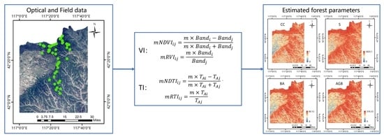
Figure 3 shows the flow chart of the proposed method.
3.1. Establishment of the Vegetation Index (VI)
The single band reflectance is susceptible to the influence of the atmosphere and the surrounding environment and has limitations in obtaining vegetation information. The vegetation index can make full use of the dominant band and eliminate the errors caused by partial single band reflectance, thus obtaining higher quality vegetation information [65]. All green plants strongly absorb visible electromagnetic radiation and reflect near-infrared radiation, and the spectral vegetation index emphasizes this difference by mathematically combining different spectral regions, which can represent the amount and condition of vegetation within a pixel [66]. Existing studies have used exhaustive methods to build vegetation indices to avoid the problems of existing vegetation indices ignoring important information that may be contained in other spectral bands and that different study areas and data producing different responses to different spectral bands [38]. It has been demonstrated that the weighting of the NIR band in the vegetation index affects the saturation point and that indices with higher weighting coefficients in the NIR band favor an increase in the sensitivity of the vegetation index [67]. However, there are fewer studies on the other bands included in different vegetation indices and the differences in response between different bands. Therefore, this study used the exhaustive method to establish the Normalized Vegetation Index () and Ratio Vegetation Index (), treating each band as the main band and the remaining bands as the secondary bands, and establishing weight for each main band, analyzing the contribution of each band to the vegetation index under different weights, and the response of different forest parameters to different bands to establish the vegetation index. After that, the relative sensitivity among vegetation indices and the sensitivity analysis with forest parameters are used to determine the optimal weight occupied by each main band and its vegetation index form.
where is the weight value, set at 0.1–1 with an interval of 0.1, is each band of the sensor, and is the other bands except .
3.2. Establishment of the Texture Index (TI)
Using spectral features alone leads to a large loss of spatial information in the image, while adding texture features makes full use of the spatial information of the image. One of the key characteristics of remote sensing images is texture, which is a crucial factor in reflecting the spatial variation in ground cover type and not only conveys the degree of roughness, but also reveals the structural details of the features as well as their relationship with the environment [68]. Different canopy regions may have various textural characteristics in the same category of remote sensing images. The canopy texture is more consistent with canopy closure and the more irregular it is, the lower the canopy closure is. The accuracy of canopy estimation will be substantially increased by selecting the right type of texture features. GLCM is the most commonly used texture analysis method to describe the correlation and spatial structure of pixel pairs according to the spatial relationship of image gray values [69]. The characteristics utilized to identify the texture cannot be directly provided by GLCM, but they can offer the gray direction and interval changes connected to the image. Therefore, it is necessary to extract the statistical attributes used to quantitatively describe the texture features based on GLCM. Textures represent the spatial arrangement of image colors or intensities, rather than image pixel values, and are more capable of expressing spatial information on the basis of vegetation indices. Texture carries significant spatial information about the arrangement of vegetation and non-vegetation surfaces in the picture and its relationship with the surrounding environment and is sensitive to canopy structural features. Vegetation indices can be used as an indicator of vegetation content, and the combination of the two provides additional information for prediction models. Therefore, the texture indices are built based on GLCM extracting texture measurements in four directions and six windows. Normalization and the ratio of bands can reduce the effects of soil background, sun angle, and sensor perspective to some extent, and texture indices combine texture measurements and normalization or ratio techniques to improve the estimation of forest parameters [58,70,71]. The texture indices following the NDVI and RVI forms, named the Normalized Texture Index () and Ratio Texture Index (), are calculated to combine the same texture features of different bands extracted from same windows with same directions. Based on the same window size and the same direction, a texture feature (A) of a single band () is taken as the main feature and the texture feature (A) of another band ) is taken as the secondary feature, and weight is established for the main feature to analyze the response differences of extracted textures between different bands, and the optimal weights and texture features are determined via the sensitivity analysis.
where, is the weight value, set 0.1–1 with an interval of 0.1, and and denote the same GLCM texture (texture feature ) extracted from different bands ( and ) in the same window with the same direction.
Because textures differ greatly depending on the environment, texture measurements, and associated characteristics (such as window size, orientation, and offset), integrating texture information for forest regions is difficult. Furthermore, texture processing might result in a significant volume of unmanageable data [72]. Therefore, this study establishes texture indices generated in three ways based on different window sizes:
- Corresponding Texture Index (CTI): Based on the same window size and the same direction, all of the texture features of each band are used as main features, and the texture features of the remaining bands that are the same as the main features are used as secondary features to establish the texture index.
- Mean Texture Index (MTI): In order to reduce the influence of the direction parameters and the dimensionality of the input variables on the modeling, the same texture features in four directions for each window of each band are averaged to avoid the influence of feature differences arising from different directions [60]. Therefore, based on the same window, all texture features of each band are used as main features, and the remaining band texture features corresponding to them are used as secondary features to build texture indices.
- Principal Component Analysis Texture Index (PTI): Since there are many textures generated in this study and there is a certain correlation between the sensor bands themselves, the correlational analysis of the texture information obtained from each band reveals that there is a relatively obvious correlation between the texture information. Therefore, the texture features obtained from each band are subjected to principal component dimensionality reduction analysis, which ensures the original information of the image texture and improves the efficiency of data computation at the same time. Based on the same window size and the same direction, the eight texture features extracted from the same band are subjected to principal component analysis, and only the first principal component is selected. Therefore, based on the same window and the same direction, the first principal component features obtained from a single band are used as the main features and the first principal component features of the remaining bands are used as secondary features to build texture indices.
3.3. Sensitivity Analysis
3.3.1. Relative Sensitivity
The results of the sensitivity analysis are more intuitive, and the vegetation index has a visual graphical and numerical expression of the magnitude of the forest parameters, which can not only evaluate the indicativeness of the vegetation index itself and between vegetation indices in general but also more accurately express the ability of the vegetation index to reflect the forest parameters. The relative sensitivity index is used to quantitatively compare the sensitivity of the improved index (the index with weight included in the main band) with the original index (the index with a weight of 1 in the main band) for different structural descriptors [73].
where and represent the new and original vegetation indices, respectively, and is the first-order derivative with respect to the forest parameter under analysis. The relative change sensitivity of the two vegetation indices is analyzed using , and , , indicate that the relative sensitivity of is less than, equal to, or greater than , respectively. The weight occupied by each main band for , i.e., the m value, is chosen to ensure that the new vegetation index has the best sensitivity.
3.3.2. Noise Equivalent Sensitivity Model
The vegetation index and texture are saturated for each forest parameter, and the vegetation index reaches saturation mainly via canopy background reflection and atmospheric effects, and this property constrains the use of the vegetation index [74]. Existing studies mostly use single evaluation indexes such as and RMSE, which cannot reflect the influence of changes in vegetation canopy on vegetation indices and only describe the overall relationship between current model variables and cannot reflect the specific influence of changes in independent variables on dependent variables, specific to the estimation of forest parameters. Therefore, some researchers have proposed vegetation index sensitivity models to further evaluate the indicative significance of vegetation indices. In this study, a noise equivalent (NE) sensitivity model is introduced to further evaluate the inversion ability of the vegetation index. The optimal main and secondary bands corresponding to each forest parameter and their weights obtained in (1) are summarized and linearly fitted to filter the optimal vegetation index using NE [75,76].
where dVId is the first-order derivative of the vegetation index with respect to the forest parameter, and the numerator is the RMSE of the fitted relationship between the two.
In addition to taking into account the RMSE of vegetation parameter estimates and the sensitivity of the vegetation index to the vegetation parameters, NE also considers the point scatter and slope of the best-fit function, providing the degree of response to vegetation parameters over the entire range of variation of the vegetation index [77]. Since weight is established for each main band texture feature, numerous texture indices are obtained. Pearson correlation coefficients are used to obtain the optimal weight values for each window corresponding to each forest parameter and the texture features of the bands. After that, the same method as that used for vegetation indices is used to filter the texture indices using NE to select the optimal window size, direction, and band corresponding texture features for each forest parameter.
4. Results
4.1. Relationship between Raw Band, Vegetation Index, Texture, and Forest Parameters
The right variables must be chosen in order to estimate various forest parameters. The linear correlation found between the characteristic variables and the forest parameters, which is the most simple and clear indicator of the relationship between these variables, is typically used to describe the availability of variables. In this study, the Pearson correlation coefficient was used to extract the bands, vegetation indices, and texture features of L8 and S2A with the best correlation with forest parameters (Table S1). The optimal results obtained for each forest parameter are shown in Table 8, and a linear relationship was established.
The results show that all forest parameters except S were significantly correlated with the SWIR bands of L8 and S2A, while S was more strongly correlated with the green band. And all forest parameters were strongly correlated with the vegetation index containing the SWIR bands [60,78]. Because the SWIR band is less susceptible to disturbances such as atmospheric absorption and scattering and has better resistance to atmospheric perturbations than the visible and NIR bands, vegetation indices that include the SWIR band have a stronger correlation with forest parameters [79]. EVI, DVI, and RDVI have a significant advantage among the many vegetation indices and accurately well the changes in vegetation cover [80]. For the CC, BA, and AGB, the texture features extracted using BTE, MTE, and PTE were mainly related to mean and correlation features, which was the same as the results in [60]. While S has different optimal texture features extracted using different methods, the texture feature that has the best correlation with S was entropy in the blue band. For textures extracted using BTE and MTE, it was mainly the medium and small window sizes that expressed better information, because the small window size is more sensitive to highly localized surface features and better captures changes in vegetation features [81]. For texture features extracted using PTE, the large window correlates better with forest parameters and is mainly associated with correlation features. The first principal component obtained after principal component analysis of the bands contains more than of the valid information of all the bands, and its extracted texture contains more information about the bands. Small windows often exaggerate the variance within the moving window, increasing the noise content on the texture image, and may not contain enough information about the region to best represent texture features with more information [82,83].
For CC, BA, and AGB, the correlation between band and vegetation indices was higher. For S, the correlation of texture features extracted using S2A was significantly higher than the other variables. Overall, S2A performed significantly better than L8, except for CC, but the optimal correlation between the two sensors and CC was not significantly different. From the scatter plot (Figure 4), although the highest was obtained for S, it was mainly limited by low forest stand density and homogeneous forest, and the texture values obtained from low forest stand density were mostly the same, limiting the estimation of S. Overall, the window was more sensitive to changes in forest parameters, and the best coefficient of determination was obtained for the texture features extracted in the direction for forest parameters.
4.2. Relationship between New Vegetation Indices and Forest Parameters
The vegetation indices containing the optimal weights were screened by means of relative sensitivity and NE sensitivity analysis, and linear models were established and compared with the corresponding forest parameters for the determination coefficients, respectively (Table S2). The results showed that the ratio index obtained by the S2A sensor gave better results with the forest parameters (Table 9). And since the SWIR band is more sensitive to vegetation information and has great potential to reflect vegetation water content and stand structure complexity, it exists in the ratio band of each parameter [84]. The SWIR is sensitive to shadows and can be a good representation of vegetation cover changes [85]. The optimal solution of S2A obtained by forest parameters contain green and red edge bands, where the green band is sensitive to canopy reflectance and the red edge, as a band specific to Sentinel-2, is sensitive to chlorophyll as well as leaf structure, providing more information for the characterization of vegetation [22,86]. A sudden increase in the reflectance of healthy vegetation can be observed in the red edge band, which can distinguish healthy vegetation from other surface features and better respond to vegetation information [87].
As can be seen from Table S2, the optimal bands extracted by the same sensor were the same for the same forest parameter, indicating that the response information of the optimal bands and the forest parameter was fixed regardless of the form of the vegetation index, but the optimal weights obtained from the bands in different forms were different, indicating that the response and the complementary relationship between the bands in different forms were different from each other, and the linear relationship with the same forest parameter was also different. Figure 5 shows the linear plot of forest parameters and the optimal vegetation index. As can be seen from Figure 6, CC, BA, and AGB achieved better results for the estimated map of the study area and generally lower results for S. Because most of the measured sample plots were concentrated in low forest stand density areas and sample plots with higher forest stand density were not explored enough, these factors limited the prediction results in the study area.
4.3. Relationship between New Texture Indices and Forest Parameters
4.3.1. CTI
The optimal texture indices for different windows, directions, and features were obtained using Pearson correlation coefficients and NE analysis, and a linear relationship was established between texture indices and forest parameters, which were then analyzed using the statistic (Table S3). The optimal results obtained for each forest parameter are shown in Table 10. The results obtained from the analysis of the CTIs showed better results for CC, S, and BA with RTIs and better results for NDTI with AGB. Except for S, the L8 sensor provides stronger information on forest parameters and mainly uses small windows because texture measurements obtained from small windows are more sensitive to fine-scale changes in pixel brightness [35]. Both CC and BA selected mean features acquired with a window and the direction angle of in SWIR. The second moment texture obtained in the direction in the window achieves better results with S, while the AGB has better results with the correlation texture extracted at the direction in the window. From the results, it is clear that the forest parameters were selected in completely different bands from the vegetation index bands, and the optimal weights established were different because of the inclusion of texture feature information.
4.3.2. MTI
The obtained MTIs were subjected to NE screening analysis, and the best MTI results screened for each sensor are shown in Table S4. The obtained optimal results are shown in Table 11. From the results, it was clear that the forest parameters were better for RTIs, and all of them were selected for the texture feature information obtained from small windows. The optimal valuses of CC, BA, and AGB were all for RTIs obtained from L8, the selected texture features were all mean textures, and the selected bands included red, NIR, and SWIR bands. These bands have enhanced reflection and absorption in the green vegetation region, and the NIR band is the peak of reflection and expresses more information. S selected the green and SWIR bands, and the selected texture was entropy. Green vegetation has a strong reflection in the green band of the electromagnetic spectrum, which better reflects the vegetation cover information [88] and SWIR can show the strongest contrast between the forest canopy and crevices (soil, apoplast) [81].
Comparative analysis with the CTI results revealed that both CC and BA selected the same bands, window sizes, and texture features, indicating that the information of both was less influenced by the direction. It can be seen that the information on CC is mainly contained in the mean texture obtained from the window of SWIR and NIR, and the information on BA is mainly contained in the mean texture of the window of red and SWIR. This shows that the mean features obtained by using the window of SWIR can effectively extract vegetation information for L8 derived textures in terms of CC and BA prediction. However, the amount of information contained in the existing texture features is different from the original texture features because the information differences in each direction are eliminated, so the optimal weights obtained are not the same, even though the corresponding bands and texture features are chosen to be the same. Both S and AGB chose different bands and texture features, indicating that S and AGB were influenced by the direction of texture feature extraction. Combined with , it is found that AGB is more suitable for the texture features obtained after averaging in multiple directions, which can better express the case of AGB, while S is more capable of obtaining information with a direction angle of and obtains better results, indicating that the variation of texture features in its single direction is stronger, and the combination with other directions weakens the information obtained in the direction.
4.3.3. PTI
It was found that the best results were obtained by subjecting each band texture feature to principal component analysis and then establishing the RTIs, and the optimal results were obtained with all of the secondary features containing more than of the information, and the amount of information contained in the main features mainly influenced , in contrast, the amount of information contained in the secondary features did not have as strong an effect on the coefficient of determination as the main features (Table 12). This study showed that the results obtained from PTIs were better than those obtained from CTIs and MTIs, indicating that individual texture features do not fully express the information on forest parameters, and that the method of principal component analysis of texture features better expresses the information contained in each texture feature, and the results obtained are significantly better than those obtained from other methods. The results show that the amount of information obtained after L8 texture PCA was less than that obtained after S2A texture PCA (Table S5). The optimal window for forest parameters was a medium window size because it is more sensitive to inter-pixel differences in the observed proportions of forest parameters than the minimum window size, which is the same as the results of Santa Pandit [89]. However, the optimal directions of each forest parameter were different, and the selected bands include green, red, NIR, and SWIR bands, which are sensitive to vegetation changes due to their strong absorption and reflection abilities of vegetation chlorophyll.
4.3.4. Image Illustration of TI Results
As can be seen from Figure 7, the values obtained by MTIs were better than those obtained by CTIs, except for S. This may be due to the fact that the average value removes the different directional differences and contains information about texture features in multiple directions. However, in terms of S, because the measured data in this study were concentrated in low forest stand density areas and all were artificial coniferous forests, the texture values may be relatively constant for artificial forests with single-storey forests of the same species, so the texture eigenvalues are more concentrated in low forest stand density areas, which may be the reason for limiting its poor results [90]. Although the of S obtained by CTI was better, its fitted straight line apparently had saturation at low stand densities, and most of the stand density estimates were the same, which did not correctly reflect the growth of stand density. The fit of AGB obtained from CTI was similar to that of S. As shown by the linear relationship between PTI and AGB, the biomass estimates of 50–100 t/ha had the same texture index values. Overall, the and linear fit results obtained by PTI for each vegetation parameter were better and showed a significant improvement in the saturated underestimation of S and AGB. As can be seen from Figure 8, the results of each forest parameter map generated using the optimal PTIs were better, and the obtained S map demonstrates a significant improvement in underestimation compared with the results estimated using the vegetation index.
5. Discussion
5.1. Sensitivity Analysis
The NE method allows the direct comparison of vegetation indices at different ranges and scales, and since this study uses linear fitting methods, the noise equivalence is constant, which is more conducive to observing the sensitivity across the entire range of forest parameters [91]. According to the meaning of the model, the smaller the NE value, the stronger the sensitivity of the vegetation index, the less affected it is by noise, and the more indicative and stable the forest parameters are [75]. The NE diagram is analyzed using CC as an example. The optimal results obtained using CC for each index were also summarized for further analysis (Table 13). Based on the NE plots of the optimal vegetation indices of CC (Figure 9), it can be seen that the ratio indices extracted with CC using S2A suffers from the lowest noise equivalent. However, according to Table 9, it can be seen that the of the RVI of L8 is better than the NDVI results obtained using S2A, but it is obvious that the optimal RVI extracted using L8 (Figure 9b) suffers from higher noise than the NDVI extracted using S2A (Figure 9c). This is because the NE considers the RMSE factor, so the NE method selects the result with the smallest RMSE rather than the largest . According to the results of each optimal index obtained by CC (Table 13), it can be seen that the RMSE of the MTI the RMSE of the VI the RMSE of the CTI the RMSE of the PTI, which corresponds to the influence of the minimum noise equivalent in each NE map (Figure 10), indicating that it is feasible to select the optimal variables for the estimation of forest parameters using NE noise maps. From the NE diagrams of vegetation indices (Figure 10a), the main bands are selected to express vegetation information in the SWIR and green bands, which can better contain vegetation cover information. The small window is subjected to less noise equivalent for CTIs (Figure 10b) and MTIs (Figure 10c), but the medium window is subjected to less noise for PTIs (Figure 10d). Most of the features extracted from the CTIs (Figure 10b) and the MTIs (Figure 10c) are means, thus indicating that the mean contains the majority of the CC information and can more accurately express the information about the vegetative changes, which also confirms the results that we obtained in Section 4.3. From the CTI diagram (Figure 10b), it can be seen that different windows of different sizes are chosen with different directions under the same band and feature conditions. From the MTI diagram (Figure 10c), the band and texture selected are exactly the same without the interference of the direction included, which indicates that different window sizes and textures affect the selection of directions differently, and also indicates that direction has less influence on the selection of band and texture.
Relative sensitivity analysis was performed using the S2A optimal vegetation index obtained from CC to analyze the causes of CC saturation by establishing the relationship between NDVI, RVI, and its components, Band3 and Band12 reflectance (Figure 11). A quadratic equation was used here for estimation, so as to better observe the saturation trend. Moreover, as quadratic equation estimation was used here, and first-order equation estimation was used in the Results section, the two results are slightly different). Band12 and CC are negatively correlated (not listed in the text), with Band12 decreasing as the forest increased. When the Band3 value is greater than 0.08, the change in Band12 value gradually becomes insensitive and reaches the asymptote at around 0.14 (Figure 11a,b). Compared with Band3, NDVI and RVI are positively correlated with Band12, without a very obvious saturation trend (Figure 11c,d). However, it can still be seen that the sensitivity of NDVI changes in Band12 starts to decrease at around 0.12. As seen in Figure 11c, the sensitivity of NDVI after adding weight is significantly better than that of the original NDVI in the CC range of 0–0.4. Comparing the results before and after increasing the weight, it is found that the value of the RMSE has improved more significantly compared to . The RVI was chosen for this study because its results were better than those of the NDVI and the improvement in RMSE was more pronounced. Meanwhile, compared to the NDVI, the RVI before and after the improvement was not significantly affected by Band12, and there was no significant saturation trend. The results show that the method of adding weight to the band of VI can effectively improve the estimated and RMSE and has a significant improvement effect on the saturation trend of NDVI.
5.2. Relationship between Raw Band, Vegetation Index, Texture Index, and Forest Parameters
The results show that the results obtained with S2A were significantly better than those obtained with L8, which is the same as the results found in existing studies [92,93,94]. The bands of each vegetation index and texture index selected by S2A are mostly concentrated in the red edge band because the leaf information of vegetation changes greatly within this range and is more sensitive to changes in the growth of vegetation. In addition, the texture and spectral bands extracted in this band range are less influenced by the surrounding environment, especially the soil factor and climate factor. The addition of the red edge band therefore plays a significant role in increasing the accuracy of the model for areas with a complicated forest stand structure [95]. Additionally, the SWIR band, green band, and red band are better predictors [94]. It was found that the SWIR band, green band, and red band were also the main selection bands for the vegetation index and texture index of L8, while the NIR band was also the main selection band for the L8 sensor. In this study, the vegetation index obtained by the Landsat 8 sensor was found to perform weakly, probably due to the presence of tall forests, whose consequent shadow effect negatively impacts the sensor’s ability to measure spectral reflectance, resulting in poor performance [35]. The results of the study in Section 4.2 show that the weight of the normalized vegetation indices was mostly 0.1, and the reason for the low sensitivity to medium and high forest stand density for NDVI is the mathematical formula of this index: the ratio of the difference to sum. The sensitivity of the NDVI depends on the ratio of the two bands, and when either band is significantly larger than the other, the numerator and denominator are nearly equivalent, and the sensitivity of the index is negligible. Therefore, creating a weighting factor for the bands in the index can narrow the gap between the contributions of the two bands to the vegetation index and improve the sensitivity to the forest parameters. The RVI uses the ratio of the two bands to determine the sensitivity. When either band is too large or too small, it affects the degree of information contribution of the other band to the RVI and reduces the sensitivity of the index.
The results of the study show that texture indices were more effective than vegetation indices in extracting vegetation information and expressing forest structure better than vegetation indices [4]. Texture features are independent of the color and brightness of the object surface and reflect the frequency of hue changes in a given window size. As a result, they are more sensitive to canopy space, which can distinguish the vegetation structure in great detail and detect different forest canopy structural characteristics [96]. The use of texture measurements that can distinguish spatial information reduces forest structure differences independent of forest parameters, and the use of complementary information for texture parameters in both bands simultaneously improves performance compared to any single texture datum. This is the same as the conclusion of previous studies [35,59,90]. The research results show that mean matches the patterns within the pixels reflecting the forest CC, BA, and AGB and reflects the texture regularity of pixels, and the larger the value is, the more obvious and easy to describe the texture pattern is [97]. Entropy and second moment are more reflective of the regularities of S, and there is a negative correlation between them which is a measure of the uniformity of grayscale distribution and represents the roughness of the texture. Second moment is a measure of the uniformity of gray distribution, indicating the roughness of the texture. The texture will be more coarse as the second moment value increases. Entropy measures the disorder or randomness of the image values, and when the gray distribution is more uneven, texture mixing is disordered, second moment is smaller, and entropy is larger [98,99]. Correlation is a measure of the linear relationship between neighboring pixels and measures the dependence of the grayscale on neighboring pixels, which implies that there is a predictable relationship between two neighboring pixels within the window and is more relevant to the distribution pattern of AGB. Combining the results of CTI and MTI shows that the optimal results for CC, BA, and AGB all come from the texture features extracted using L8, whose good performance regarding its texture metrics can be attributed to its push-scan design, which perfects the signal-to-noise ratio, and its high radiometric resolution of 12 bits makes it more sensitive and robust in detecting vegetation structures. At the same time, the refined spectral band of L8 eliminates the absorption effect of water vapor, thus allowing accurate surface spectroscopic detection [35].
This study found that the best results were obtained for the ratio indices, either VIs or TIs. The use of the ratio technique provides us with complementarity and advantages in reducing other effects such as forest structure differences, incidence angle differences, and topographic effects. Because of the heterogeneity of species and forest structure and the complexity of topography, using these advantages of ratio techniques may be particularly effective in the study area [100,101]. The results of this study show that the CTI and the MTI focus more on representing variation within objects (within crowns and shadows), as their results are selected for smaller windows, while the PTI focuses on representing variation between objects (between crown or canopy objects and canopy shadows), and therefore texture features are selected for larger windows [102].
6. Conclusions
In this study, the response characteristics between different bands and textures are used and combined with normalization and ratio techniques to effectively extend the linear relationship between variables and forest parameters, avoiding to some extent the saturation problem arising between optical sensors and forest parameters. The newly developed indices and forest parameters produced better results when compared to spectral bands, popular vegetation indices, and textures. The results show that the form of the vegetation index has no effect on the response information between spectral bands and vegetation characteristics, but that it does have an impact on the weight. The vegetation ratio index and texture ratio index developed using S2A produced the best results. The ratio technique better eliminated sensor and terrain effects, and adding weight to the ratio index based on band and texture sensitivity can effectively improve the response differences in the bands and textures, enhancing the sensitivity of the index. However, different bands and texture features contain different information, which will affect the magnitude of the weight. In this paper, by combining the principal component analysis with the texture ratio technique and adding appropriate weight according to the sensitivity between different texture features, more valid information can be retained while reducing the dimensionality of the data. The results show that variables containing more information amount of texture features have better estimation performance, and using a single texture feature does not reflect the variation of each forest parameter well. In addition, the selection of different windows and texture features can affect the selection direction differently. The results demonstrate that CC, BA, and AGB are less affected by direction, and removing the differences in direction can improve the estimation performance of forest parameters, but S is more affected by direction and has the strongest response to the texture features in the direction. S is also associated with the orderliness based texture features, and CC, BA, and AGB are associated with statistically based texture features.
The study area comprises artificial coniferous forests, and the main tree species are Larix principis-rupprechtii Mayr and Pinus sylvestris var. mongholica Litv, so most of the areas have similar spectral characteristics. Because optical canopy reflectance depends on a complex interaction of internal and external factors and most stand features are spatially and temporally dependent, and because the remote sensing data and sample site data in this study are not perfectly matched in time, which may vary significantly in time and space. Therefore, empirical relationships will vary by location, time, and species type and are not directly applicable to large-scale operational use. In addition, this study uses only optical data, which can only obtain surface features of forest structure, and it is expected that combining SAR or LiDAR data to combine vertical structure information can obtain better results.
Supplementary Materials
The following supporting information can be downloaded at: https://www.mdpi.com/article/10.3390/rs15143605/s1. Table S1. The results of band, vegetation index, texture and forest parameters; Table S2. The results of VI and forest parameters; Table S3. The results of CTI and forest parameters; Table S4. The results of MTI and forest parameters; Table S5. The results of PTI and forest parameters.
Author Contributions
Conceptualization, W.F. and R.S.; methodology, R.S.; software, R.S.; validation, R.S.; formal analysis, R.S.; investigation, R.S.; resources, W.F.; data curation, R.S.; writing—original draft preparation, R.S.; writing—review and editing, R.S.; visualization, R.S. All authors have read and agreed to the published version of the manuscript.
Funding
This research was funded by the National Natural Science Foundation of China (contract no. 31971654) and the Civil Aerospace Technology Advance Research Project (contract no. D040114).
Conflicts of Interest
Declare no conflict of interest or state. The funders had no role in the design of the study; in the collection, analyses, or interpretation of data; in the writing of the manuscript; or in the decision to publish the results.
References
- Oliveira, C.; Luiz, R.; Silva, J.; Lima, R.; Silva, E.; da Silva, A.; Lucena, J.; Tavares dos Santos, N.; Lopes, I.; Pessoa, M.; et al. Modeling and Spatialization of Biomass and Carbon Stock Using LiDAR Metrics in Tropical Dry Forest, Brazil. Forests 2021, 12, 473. [Google Scholar] [CrossRef]
- Chen, W.; Zheng, Q.; Xiang, H.; Chen, X.; Sakai, T. Forest Canopy Height Estimation Using Polarimetric Interferometric Synthetic Aperture Radar (PolInSAR) Technology Based on Full-Polarized ALOS/PALSAR Data. Remote Sens. 2021, 13, 174. [Google Scholar] [CrossRef]
- Ingram, J.C.; Dawson, T.P.; Whittaker, R.J. Mapping tropical forest structure in southeastern Madagascar using remote sensing and artificial neural networks. Remote Sens. Environ. 2005, 94, 491–507. [Google Scholar] [CrossRef]
- Eckert, S. Improved Forest Biomass and Carbon Estimations Using Texture Measures from WorldView-2 Satellite Data. Remote Sens. 2012, 4, 810–829. [Google Scholar] [CrossRef] [Green Version]
- Ehlers, D.; Wang, C.; Coulston, J.; Zhang, Y.; Pavelsky, T.; Frankenberg, E.; Woodcock, C.; Song, C. Mapping Forest Aboveground Biomass Using Multisource Remotely Sensed Data. Remote Sens. 2022, 14, 1115. [Google Scholar] [CrossRef]
- Li, C.; Li, Y.; Li, M. Improving Forest Aboveground Biomass (AGB) Estimation by Incorporating Crown Density and Using Landsat 8 OLI Images of a Subtropical Forest in Western Hunan in Central China. Forests 2019, 10, 104. [Google Scholar] [CrossRef] [Green Version]
- Williams, M.; Mitchell, A.; Milne, A.K.; Danaher, T.; Horn, G. Addressing critical influences on L-band radar backscatter for improved estimates of basal area and change. Remote Sens. Environ. 2022, 272, 112933. [Google Scholar] [CrossRef]
- Stelmaszczuk-Gorska, M.; Rodriguez-Veiga, P.; Ackermann, N.; Thiel, C.; Balzter, H.; Schmullius, C. Non-Parametric Retrieval of Aboveground Biomass in Siberian Boreal Forests with ALOS PALSAR Interferometric Coherence and Backscatter Intensity. J. Imaging 2016, 2, 1. [Google Scholar] [CrossRef] [Green Version]
- Urbazaev, M.; Thiel, C.; Migliavacca, M.; Reichstein, M.; Rodriguez-Veiga, P.; Schmullius, C. Improved Multi-Sensor Satellite-Based Aboveground Biomass Estimation by Selecting Temporally Stable Forest Inventory Plots Using NDVI Time Series. Forests 2016, 7, 169. [Google Scholar] [CrossRef]
- Ahmed, R.; Siqueira, P.; Hensley, S. Analyzing the Uncertainty of Biomass Estimates From L-Band Radar Backscatter Over the Harvard and Howland Forests. IEEE Trans. Geosci. Remote Sens. 2014, 52, 3568–3586. [Google Scholar] [CrossRef]
- Lu, D. The Potential and Challenge of Remote Sensing–Based Biomass Estimation. Int. J. Remote Sens. 2006, 27, 1297–1328. [Google Scholar] [CrossRef]
- Günlü, A.; Ercanli, I.; Şenyurt, M.; Keleş, S. Estimation of some stand parameters from textural features from WorldView-2 satellite image using the artificial neural network and multiple regression methods: A case study from Turkey. Geocarto Int. 2019, 36, 918–935. [Google Scholar] [CrossRef]
- Zhang, H.; Wang, C.; Zhu, J.; Fu, H.; Xie, Q.; Shen, P. Forest Above-Ground Biomass Estimation Using Single-Baseline Polarization Coherence Tomography with P-Band PolInSAR Data. Forests 2018, 9, 163. [Google Scholar] [CrossRef] [Green Version]
- Chen, L.; Ren, C.; Zhang, B.; Wang, Z.; Xi, Y. Estimation of Forest Above-Ground Biomass by Geographically Weighted Regression and Machine Learning with Sentinel Imagery. Forests 2018, 9, 582. [Google Scholar] [CrossRef] [Green Version]
- Timothy, D.; Onisimo, M.; Cletah, S.; Adelabu, S.; Tsitsi, B. Remote sensing of aboveground forest biomass: A review. Trop. Ecol. 2016, 57, 125–132. [Google Scholar]
- Lu, D.; Batistella, M. Exploring TM Image Texture and Its Relationships with Biomass Estimation in Rondônia, Brazilian Amazon. Acta Amaz. 2005, 35, 249–257. [Google Scholar] [CrossRef]
- Dogru, A.; Göksel, Ç.; David, R.-M.; Tolunay, D.; Sözen, S.; Orhon, D. Detrimental environmental impact of large scale land use through deforestation and deterioration of carbon balance in Istanbul Northern Forest Area. Environ. Earth Sci. 2020, 79, 270. [Google Scholar] [CrossRef]
- Phiri, D.; Morgenroth, J. Developments in Landsat Land Cover Classification Methods: A Review. Remote Sens. 2017, 9, 967. [Google Scholar] [CrossRef] [Green Version]
- Gizachew, B.; Solberg, S.; Næsset, E.; Gobakken, T.; Bollandsås, O.M.; Breidenbach, J.; Zahabu, E.; Mauya, E.W. Mapping and estimating the total living biomass and carbon in low-biomass woodlands using Landsat 8 CDR data. Carbon Balance Manag. 2016, 11, 13. [Google Scholar] [CrossRef] [Green Version]
- David, R.M.; Rosser, N.J.; Donoghue, D.N.M. Improving above ground biomass estimates of Southern Africa dryland forests by combining Sentinel-1 SAR and Sentinel-2 multispectral imagery. Remote Sens. Environ. 2022, 282, 113232. [Google Scholar] [CrossRef]
- Jiang, F.; Kutia, M.; Sarkissian, A.J.; Lin, H.; Long, J.; Sun, H.; Wang, G. Estimating the Growing Stem Volume of Coniferous Plantations Based on Random Forest Using an Optimized Variable Selection Method. Sensors 2020, 20, 7248. [Google Scholar] [CrossRef]
- Jiang, F.; Sun, H.; Chen, E.; Wang, T.; Cao, Y.; Liu, Q. Above-Ground Biomass Estimation for Coniferous Forests in Northern China Using Regression Kriging and Landsat 9 Images. Remote Sens. 2022, 14, 5734. [Google Scholar] [CrossRef]
- Li, J.; Mao, X. Comparison of Canopy Closure Estimation of Plantations Using Parametric, Semi-Parametric, and Non-Parametric Models Based on GF-1 Remote Sensing Images. Forests 2020, 11, 597. [Google Scholar] [CrossRef]
- Chen, Y.; Li, L.; Lu, D.; Li, D. Exploring Bamboo Forest Aboveground Biomass Estimation Using Sentinel-2 Data. Remote Sens. 2018, 11, 7. [Google Scholar] [CrossRef] [Green Version]
- Lu, D.; Chen, Q.; Wang, G.; Liu, L.; Li, G.; Moran, E. A survey of remote sensing-based aboveground biomass estimation methods in forest ecosystems. Int. J. Digit. Earth 2016, 9, 63–105. [Google Scholar] [CrossRef]
- Lima-Cueto, F.J.; Blanco-Sepúlveda, R.; Gómez-Moreno, M.L.; Galacho-Jiménez, F.B. Using Vegetation Indices and a UAV Imaging Platform to Quantify the Density of Vegetation Ground Cover in Olive Groves (Olea europaea L.) in Southern Spain. Remote Sens. 2019, 11, 2564. [Google Scholar] [CrossRef] [Green Version]
- Delpasand, S.; Bahmankiani; Mokhtari, M. Evaluation of the capability of Landsat 8 data for predicting tree density in the Bagh-ShadiHarat forests. Adv. Environ. Biol. 2014, 8, 1449–1452. [Google Scholar]
- Günlü, A.; Ercanli, I.; Başkent, E.; Çakir, G. Estimating aboveground biomass using Landsat TM imagery: A case study of Anatolian Crimean pine forests in Turkey. Ann. For. Res. 2014, 57, 289–298. [Google Scholar] [CrossRef]
- Nouri, A.; Kiani, B.; Hakimi, M.H.; Mokhtari, M.H. Estimating oak forest parameters in the western mountains of Iran using satellite-based vegetation indices. J. For. Res. 2020, 31, 541–552. [Google Scholar] [CrossRef]
- Lu, D.; Mausel, P.; Brondízio, E.; Moran, E. Relationships between forest stand parameters and Landsat TM spectral responses in the Brazilian Amazon Basin. For. Ecol. Manag. 2004, 198, 149–167. [Google Scholar] [CrossRef]
- Forkuor, G.; Dimobe, K.; Serme, I.; Tondoh, E. Landsat-8 vs. Sentinel-2: Examining the added value of sentinel-2’s red-edge bands to land-use and land-cover mapping in Burkina Faso. GIScience Remote Sens. 2017, 55, 331–354. [Google Scholar] [CrossRef]
- Chen, J.-C.; Yang, C.M.; Wu, S.-T.; Chung, Y.L.; Charles, A.L.; Chen, C.-T. Leaf chlorophyll content and surface spectral reflectance of tree species along a terrain gradient in Taiwan’s Kenting National Park. Bot. Stud. 2007, 48, 71–77. [Google Scholar]
- Zhao, D.; Huang, L.; Li, J.; Qi, J. A comparative analysis of broadband and narrowband derived vegetation indices in predicting LAI and CCD of a cotton canopy. ISPRS J. Photogramm. Remote Sens. 2007, 62, 25–33. [Google Scholar] [CrossRef]
- Linjing, Z.; Zhenfeng, S.; Zhiguo, W. Estimation of forest aboveground biomass using the integration of spectral and textural features from GF-1 satellite image. In Proceedings of the 2016 4th International Workshop on Earth Observation and Remote Sensing Applications (EORSA), Guangzhou, China, 4–6 July 2016; pp. 353–357. [Google Scholar]
- Dube, T.; Mutanga, O. Investigating the robustness of the new Landsat-8 Operational Land Imager derived texture metrics in estimating plantation forest aboveground biomass in resource constrained areas. ISPRS J. Photogramm. Remote Sens. 2015, 108, 12–32. [Google Scholar] [CrossRef]
- Zhen, Z.; Chen, S.; Yin, T.; Chavanon, E.; Lauret, N.; Guilleux, J.; Henke, M.; Qin, W.; Cao, L.; Li, J.; et al. Using the Negative Soil Adjustment Factor of Soil Adjusted Vegetation Index (SAVI) to Resist Saturation Effects and Estimate Leaf Area Index (LAI) in Dense Vegetation Areas. Sensors 2021, 21, 2115. [Google Scholar] [CrossRef]
- Stratoulias, D.; Tóth, V. Photophysiology and Spectroscopy of Sun and Shade Leaves of Phragmites australis and the Effect on Patches of Different Densities. Remote Sens. 2020, 12, 200. [Google Scholar] [CrossRef] [Green Version]
- Stratoulias, D.; Nuthammachot, N.; Suepa, T.; Phoungthong, K. Assessing the Spectral Information of Sentinel-1 and Sentinel-2 Satellites for Above-Ground Biomass Retrieval of a Tropical Forest. ISPRS Int. J. Geo-Inf. 2022, 11, 199. [Google Scholar] [CrossRef]
- Ozdemir, I.; Karnieli, A. Predicting forest structural parameters using the image texture derived from WorldView-2 multispectral imagery in a dryland forest, Israel. Int. J. Appl. Earth Obs. Geoinf. 2011, 13, 701–710. [Google Scholar] [CrossRef]
- Kayitakire, F.; Hamel, C.; Defourny, P. Retrieving forest structure variables based on image texture analysis and IKONOS-2 imagery. Remote Sens. Environ. 2006, 102, 390–401. [Google Scholar] [CrossRef]
- Sarker, L.R.; Nichol, J.E. Improved forest biomass estimates using ALOS AVNIR-2 texture indices. Remote Sens. Environ. 2011, 115, 968–977. [Google Scholar] [CrossRef]
- Hlatshwayo, S.T.; Mutanga, O.; Lottering, R.T.; Kiala, Z.; Ismail, R. Mapping forest aboveground biomass in the reforested Buffelsdraai landfill site using texture combinations computed from SPOT-6 pan-sharpened imagery. Int. J. Appl. Earth Obs. Geoinf. 2019, 74, 65–77. [Google Scholar] [CrossRef]
- Xiaoyan, F.; Dayong, J.; Lihua, W.; Xingjiu, G.; Dong, Q. Study on biomass of Larix principis-rupprechtii in Saihanba Mechanized Forestry Centre. Hebei J. For. Orchard. Res. 2015, 30, 113–116. [Google Scholar] [CrossRef]
- Xiaosha, L.; Congying, C.; Zhongqi, X.; Lin, M.; Yan, Z.; Qiang, W.; Shun, C.; Tongxiang, C. The biomass of Scotch pine plantations in Saihanba area of Hebei province. Hebei J. For. Orchard. Res. 2016, 31, 230–234. [Google Scholar] [CrossRef]
- Wang, Z.; Feng, Z. On Estimating the Parameters of Tree Biomass Using Nonlinear LS. J. Jilin Agric. Univ. 2006, 28, 261–264. [Google Scholar] [CrossRef]
- Puliti, S.; Breidenbach, J.; Schumacher, J.; Hauglin, M.; Klingenberg, T.F.; Astrup, R. Above-ground biomass change estimation using national forest inventory data with Sentinel-2 and Landsat. Remote Sens. Environ. 2021, 265, 112644. [Google Scholar] [CrossRef]
- Martín-Ortega, P.; García-Montero, L.G.; Sibelet, N. Temporal Patterns in Illumination Conditions and Its Effect on Vegetation Indices Using Landsat on Google Earth Engine. Remote Sens. 2020, 12, 211. [Google Scholar] [CrossRef] [Green Version]
- Banerjee, B.; Spangenberg, G.; Kant, S. Fusion of Spectral and Structural Information from Aerial Images for Improved Biomass Estimation. Remote Sens. 2020, 12, 3164. [Google Scholar] [CrossRef]
- Bannari, A.; Morin, D.; Bonn, F.; Huete, A.R. A review of vegetation indices. Remote Sens. Rev. 1995, 13, 95–120. [Google Scholar] [CrossRef]
- Huete, A.R.; Liu, H.Q.; Batchily, K.; van Leeuwen, W. A comparison of vegetation indices over a global set of TM images for EOS-MODIS. Remote Sens. Environ. 1997, 59, 440–451. [Google Scholar] [CrossRef]
- Roujean, J.-L.; Breon, F.-M. Estimating PAR absorbed by vegetation from bidirectional reflectance measurements. Remote Sens. Environ. 1995, 51, 375–384. [Google Scholar] [CrossRef]
- Huete, A.R. A soil-adjusted vegetation index (SAVI). Remote Sens. Environ. 1988, 25, 295–309. [Google Scholar] [CrossRef]
- Rondeaux, G.; Steven, M.; Baret, F. Optimization of soil-adjusted vegetation indices. Remote Sens. Environ. 1996, 55, 95–107. [Google Scholar] [CrossRef]
- Kaufman, Y.J.; Tanre, D. Atmospherically resistant vegetation index (ARVI) for EOS-MODIS. IEEE Trans. Geosci. Remote Sens. 1992, 30, 261–270. [Google Scholar] [CrossRef]
- Crippen, R. Calculating the vegetation index faster. Remote Sens. Environ. 1990, 34, 71–73. [Google Scholar] [CrossRef]
- Chen, J.M. Evaluation of Vegetation Indices and a Modified Simple Ratio for Boreal Applications. Can. J. Remote Sens. 1996, 22, 229–242. [Google Scholar] [CrossRef]
- Goel, N.S.; Qin, W. Influences of canopy architecture on relationships between various vegetation indices and LAI and Fpar: A computer simulation. Remote Sens. Rev. 1994, 10, 309–347. [Google Scholar] [CrossRef]
- Zheng, H.; Cheng, T.; Zhou, M.; Li, D.; Yao, X.; Tian, Y.; Cao, W.; Zhu, Y. Improved estimation of rice aboveground biomass combining textural and spectral analysis of UAV imagery. Precis. Agric. 2019, 20, 611–629. [Google Scholar] [CrossRef]
- Solórzano, J.V.; Meave, J.A.; Gallardo-Cruz, J.A.; González, E.J.; Hernández-Stefanoni, J.L. Predicting old-growth tropical forest attributes from very high resolution (VHR)-derived surface metrics. Int. J. Remote Sens. 2017, 38, 492–513. [Google Scholar] [CrossRef]
- Li, C.; Zhou, L.; Xu, W. Estimating Aboveground Biomass Using Sentinel-2 MSI Data and Ensemble Algorithms for Grassland in the Shengjin Lake Wetland, China. Remote Sens. 2021, 13, 1595. [Google Scholar] [CrossRef]
- Mingchang, W. Exploring the Optimal Feature Combination of Tree Species Classification by Fusing Multi-Feature and Multi-Temporal Sentinel-2 Data in Changbai Mountain. Forests 2022, 13, 1058. [Google Scholar] [CrossRef]
- Zhang, L.; Cheng, Q.; Li, C. Improved model for estimating the biomass of Populus euphratica forest using the integration of spectral and textural features from the Chinese high-resolution remote sensing satellite GaoFen-1. J. Appl. Remote Sens. 2015, 9, 096010. [Google Scholar] [CrossRef]
- Gini, R.; Sona, G.; Ronchetti, G.; Passoni, D.; Pinto, L. Improving Tree Species Classification Using UAS Multispectral Images and Texture Measures. ISPRS Int. J. Geo-Inf. 2018, 7, 315. [Google Scholar] [CrossRef] [Green Version]
- Haralick, R.M.; Shanmugam, K.; Dinstein, I. Textural Features for Image Classification. IEEE Trans. Syst. Man Cybern. 1973, SMC-3, 610–621. [Google Scholar] [CrossRef] [Green Version]
- Wanxue, Z.; Shiji, L.; Xubo, Z.; Yang, L.; Zhigang, S. Estimation of winter wheat yield using optimal vegetation indices from unmanned aerial vehicle remote sensing. Trans. Chin. Soc. Agric. Eng. 2018, 34, 78–86. [Google Scholar] [CrossRef]
- Castillo-Santiago, M.; Ricker, M.; Jong, B. Estimation of tropical forest structure from SPOT5 satellite images. Int. J. Remote. Sens. 2010, 31, 2767–2782. [Google Scholar] [CrossRef]
- Huete, A.; Liu, H.; Van Leeuwen, W. The use of vegetation indices in forested regions: Issues of linearity and saturation. In Proceedings of the IEEE International Geoscience and Remote Sensing Symposium, Singapore, 3–8 August 1997; Volume 4, pp. 1966–1968. [Google Scholar]
- Chi, L. The Estimation and Dynamic Modeling on the Aboveground Biomass of Pinus Densata in Shangri-La Based on Landsat. Master’s Thesis, Southwest Forestry University, Kunming, China, 2017. [Google Scholar]
- Zhang, R.; Li, Q.; Duan, K.F.; You, S.C.; Zhang, T.; Liu, K.; Gan, Y.H. Precise Classification of Forest Species Based on Multi-Source Remote-Sensing Images. Appl. Ecol. Environ. Res. 2020, 18, 3659–3681. [Google Scholar] [CrossRef]
- Zhang, J.; Qiu, X.; Wu, Y.; Zhu, Y.; Cao, Q.; Liu, X.-J.; Cao, W. Combining texture, color, and vegetation indices from fixed-wing UAS imagery to estimate wheat growth parameters using multivariate regression methods. Comput. Electron. Agric. 2021, 185, 106138. [Google Scholar] [CrossRef]
- Zhang, X.; Zhang, K.; Sun, Y.; Zhao, Y.; Zhuang, H.; Wei, B.; Chen, Y.; Fu, E.; Chen, S.; Liu, J.; et al. Combining Spectral and Texture Features of UAS-Based Multispectral Images for Maize Leaf Area Index Estimation. Remote Sens. 2022, 14, 331. [Google Scholar] [CrossRef]
- Chrysafis, I.; Mallinis, G.; Tsakiri, M.; Patias, P. Evaluation of single-date and multi-seasonal spatial and spectral information of Sentinel-2 imagery to assess growing stock volume of a Mediterranean forest. Int. J. Appl. Earth Obs. Geoinf. 2019, 77, 1–14. [Google Scholar] [CrossRef]
- Gitelson, A.A. Wide Dynamic Range Vegetation Index for remote quantification of biophysical characteristics of vegetation. J. Plant Physiol. 2004, 161, 165–173. [Google Scholar] [CrossRef] [Green Version]
- Bégué, A. Leaf area index, intercepted photosynthetically active radiation, and spectral vegetation indices: A sensitivity analysis for regular-clumped canopies. Remote Sens. Environ. 1993, 46, 45–59. [Google Scholar] [CrossRef]
- Nguy-Robertson, A.; Gitelson, A.; Peng, Y.; Viña, A.; Arkebauer, T.; Rundquist, D. Green Leaf Area Index Estimation in Maize and Soybean: Combining Vegetation Indices to Achieve Maximal Sensitivity. Agron. J. 2012, 104, 1336–1347. [Google Scholar] [CrossRef] [Green Version]
- Viña, A.; Gitelson, A. New developments in the remote estimation of the fraction of absorbed photosynthtically active radiation in crops. Geophys. Res. Lett. 2005, 32, L17403. [Google Scholar] [CrossRef] [Green Version]
- Gitelson, A.A. Remote estimation of crop fractional vegetation cover: The use of noise equivalent as an indicator of performance of vegetation indices. Int. J. Remote Sens. 2013, 34, 6054–6066. [Google Scholar] [CrossRef]
- Dang, A.; Nandy, S.; Srinet, R.; Nguyen Viet, L.; Ghosh, S.; Kumar, S. Forest aboveground biomass estimation using machine learning regression algorithm in Yok Don National Park, Vietnam. Ecol. Inform. 2018, 50, 24–32. [Google Scholar] [CrossRef]
- Lin, C.; Daoli, P.; Xuejun, W.; Xinyun, C. Estimation of Forest Stock Volume with Spectral and Textural Information from the Sentinel-2A. J. Northeast. For. Univ. 2018, 46, 54–58. [Google Scholar] [CrossRef]
- Chen, G.; Lou, T.; Jing, W.; Wang, Z. Sparkpr: An Efficient Parallel Inversion of Forest Canopy Closure. IEEE Access 2019, 7, 135949–135956. [Google Scholar] [CrossRef]
- Asner, G.; Keller, M.; Pereira, R.; Zweede, J. Remote sensing of selective logging in Amazonia: Assessing limitations based on detailed field observations, Landsat ETM+, and textural analysis. Remote Sens. Environ. 2002, 80, 483–496. [Google Scholar] [CrossRef]
- Lu, D. Aboveground biomass estimation using Landsat TM data in the Brazilian Amazon. Int. J. Remote Sens. 2005, 26, 2509–2525. [Google Scholar] [CrossRef]
- Meng, J.; Li, S.; Wang, W.; Liu, Q.; Xie, S.; Ma, W. Mapping Forest Health Using Spectral and Textural Information Extracted from SPOT-5 Satellite Images. Remote Sens. 2016, 8, 719. [Google Scholar] [CrossRef] [Green Version]
- Wang, Y.; Zhang, X.; Guo, Z. Estimation of tree height and aboveground biomass of coniferous forests in North China using stereo ZY-3, multispectral Sentinel-2, and DEM data. Ecol. Indic. 2021, 126, 107645. [Google Scholar] [CrossRef]
- Pham, T.D.; Yokoya, N.; Bui, D.; Yoshino, K.; Friess, D. Remote Sensing Approaches for Monitoring Mangrove Species, Structure, and Biomass: Opportunities and Challenges. Remote Sens. 2019, 11, 230. [Google Scholar] [CrossRef] [Green Version]
- Sibanda, M.; Mutanga, O.; Rouget, M.; Kumar, L. Estimating Biomass of Native Grass Grown under Complex Management Treatments Using WorldView-3 Spectral Derivatives. Remote Sens. 2017, 9, 55. [Google Scholar] [CrossRef] [Green Version]
- Behera, M.D.; Barnwal, S.; Paramanik, S.; Das, P.; Bhattyacharya, B.K.; Jagadish, B.; Roy, P.S.; Ghosh, S.M.; Behera, S.K. Species-Level Classification and Mapping of a Mangrove Forest Using Random Forest—Utilisation of AVIRIS-NG and Sentinel Data. Remote Sens. 2021, 13, 2027. [Google Scholar] [CrossRef]
- Pu, R.; Landry, S. Evaluating seasonal effect on forest leaf area index mapping using multi-seasonal high resolution satellite pléiades imagery. Int. J. Appl. Earth Obs. Geoinf. 2019, 80, 268–279. [Google Scholar] [CrossRef]
- Pandit, S.; Tsuyuki, S.; Dube, T. Exploring the inclusion of Sentinel-2 MSI texture metrics in above-ground biomass estimation in the community forest of Nepal. Geocarto Int. 2019, 35, 1832–1849. [Google Scholar] [CrossRef]
- Lee, Y.-S.; Lee, S.; Baek, W.-K.; Jung, H.-S.; Park, S.-H.; Lee, M.-J. Mapping Forest Vertical Structure in Jeju Island from Optical and Radar Satellite Images Using Artificial Neural Network. Remote Sens. 2020, 12, 797. [Google Scholar] [CrossRef] [Green Version]
- Viña, A.; Gitelson, A.A.; Nguy-Robertson, A.L.; Peng, Y. Comparison of different vegetation indices for the remote assessment of green leaf area index of crops. Remote Sens. Environ. 2011, 115, 3468–3478. [Google Scholar] [CrossRef]
- Ahmadi, K.; Kalantar, B.; Saeidi, V.; Harandi, E.K.G.; Janizadeh, S.; Ueda, N. Comparison of Machine Learning Methods for Mapping the Stand Characteristics of Temperate Forests Using Multi-Spectral Sentinel-2 Data. Remote Sens. 2020, 12, 3019. [Google Scholar] [CrossRef]
- Sibanda, M.; Mutanga, O.; Rouget, M. Examining the potential of Sentinel-2 MSI spectral resolution in quantifying above ground biomass across different fertilizer treatments. ISPRS J. Photogramm. Remote Sens. 2015, 110, 55–65. [Google Scholar] [CrossRef]
- Astola, H.; Häme, T.; Sirro, L.; Molinier, M.; Kilpi, J. Comparison of Sentinel-2 and Landsat 8 imagery for forest variable prediction in boreal region. Remote Sens. Environ. 2019, 223, 257–273. [Google Scholar] [CrossRef]
- Yongfeng, J. Estimation of Tree Biomass in Hubei Province by Coupling Optical Image Data and Topographic Factors. Master’s Thesis, Huazhong Agricultural University, Wuhan, China, 2021. [Google Scholar]
- Zhang, C.; Huang, C.; Li, H.; Liu, Q.; Li, J.; Bridhikitti, A.; Liu, G. Effect of Textural Features in Remote Sensed Data on Rubber Plantation Extraction at Different Levels of Spatial Resolution. Forests 2020, 11, 399. [Google Scholar] [CrossRef] [Green Version]
- Xiyuan, W.; Wangfei, Z.; Yun, L.; Xianbao, Y. Estimation of Forest Above-ground Biomass from Optical Remote Sensing Databy Optimizing Features. J. Northeast. For. Univ. 2022, 50, 47–54. [Google Scholar] [CrossRef]
- Hasituya; Chen, Z.; Wang, L.; Wu, W.; Jiang, Z.; Li, H. Monitoring Plastic-Mulched Farmland by Landsat-8 OLI Imagery Using Spectral and Textural Features. Remote Sens. 2016, 8, 353. [Google Scholar] [CrossRef] [Green Version]
- Fang, F.; McNeil, B.E.; Warner, T.A.; Maxwell, A.E. Combining high spatial resolution multi-temporal satellite data with leaf-on LiDAR to enhance tree species discrimination at the crown level. Int. J. Remote Sens. 2018, 39, 9054–9072. [Google Scholar] [CrossRef]
- Thapa, R.; Watanabe, M.; Motohka, T.; Shimada, M. Potential of high-resolution ALOS–PALSAR mosaic texture for aboveground forest carbon tracking in tropical region. Remote Sens. Environ. 2015, 160, 122–133. [Google Scholar] [CrossRef]
- Sarker, M.; Nichol, J.; Iz, H.; Ahmad, B.B.; Rahman, A. Forest Biomass Estimation Using Texture Measurements of High-Resolution Dual-Polarization C-Band SAR Data. IEEE Trans. Geosci. Remote Sens. 2013, 51, 3371–3384. [Google Scholar] [CrossRef]
- Pasher, J.; King, D. Multivariate forest structure modelling and mapping using high resolution airborne imagery and topographic information. Remote Sens. Environ. 2010, 114, 1718–1732. [Google Scholar] [CrossRef]
Figure 1.
Location map of the study area, with the actual sample locations indicated by green dots. The image of the study area is a true color image of Sentinel-2A.
Figure 1.
Location map of the study area, with the actual sample locations indicated by green dots. The image of the study area is a true color image of Sentinel-2A.

Figure 2.
Relationships between forest structural parameters at the sample site level. (a) mean DBH vs. S, (b) CC vs. BA, where the size and color shade of the dots varies with biomass.
Figure 2.
Relationships between forest structural parameters at the sample site level. (a) mean DBH vs. S, (b) CC vs. BA, where the size and color shade of the dots varies with biomass.

Figure 3.
Flow chart of the method used in this study.

Figure 4.
One-dimensional linear plot of the optimal variables obtained after Pearson correlation coefficient screening, with each forest parameter. The horizontal axis is each forest parameter, and the vertical axis is the optimal variable extracted from each forest parameter.
Figure 4.
One-dimensional linear plot of the optimal variables obtained after Pearson correlation coefficient screening, with each forest parameter. The horizontal axis is each forest parameter, and the vertical axis is the optimal variable extracted from each forest parameter.

Figure 5.
Diagram of linear relationship between forest parameters and the optimal vegetation indices fit.
Figure 5.
Diagram of linear relationship between forest parameters and the optimal vegetation indices fit.

Figure 6.
Map of forest parameters in the study area using vegetation indices estimation.

Figure 7.
Summary plot of texture indices: the optimal texture indices obtained for each vegetation parameter and their fitted linear plots. The vegetation parameters from left to right are: CC, S, BA, and AGB, and the texture indices from top to bottom are: CTI, MTI, and PTI.
Figure 7.
Summary plot of texture indices: the optimal texture indices obtained for each vegetation parameter and their fitted linear plots. The vegetation parameters from left to right are: CC, S, BA, and AGB, and the texture indices from top to bottom are: CTI, MTI, and PTI.

Figure 8.
Map of forest parameters in the study area obtained by means of PTI estimation.

Figure 9.
NE diagrams of optimal vegetation index obtained using CC. (a) NDVI extracted from L8, (b) RVI extracted from L8, (c) NDVI extracted from S2A, and (d) RVI extracted from S2A. The vertical axis of each graph is marked with the minimum NE value, and the line subject to the minimum NE value is emboldened in the graph.

Figure 10.
Summary of NE plots of the optimal vegetation index and texture index obtained via CC. (a) VI, (b) CTI, (c) MTI, and (d) PTI. The vertical axis of each graph is marked with the minimum NE value, and the line subject to the minimum NE value is emboldened in the graph.
Figure 10.
Summary of NE plots of the optimal vegetation index and texture index obtained via CC. (a) VI, (b) CTI, (c) MTI, and (d) PTI. The vertical axis of each graph is marked with the minimum NE value, and the line subject to the minimum NE value is emboldened in the graph.

Figure 11.
(a) Fit of Band3, Band12 and NDVI for Sentinel-2A. (b) Fit of Band3, Band12 and RVI. (c) Fit of CC with NDVI before and after improvement. (d) Fit of CC with RVI before and after improvement.
Figure 11.
(a) Fit of Band3, Band12 and NDVI for Sentinel-2A. (b) Fit of Band3, Band12 and RVI. (c) Fit of CC with NDVI before and after improvement. (d) Fit of CC with RVI before and after improvement.


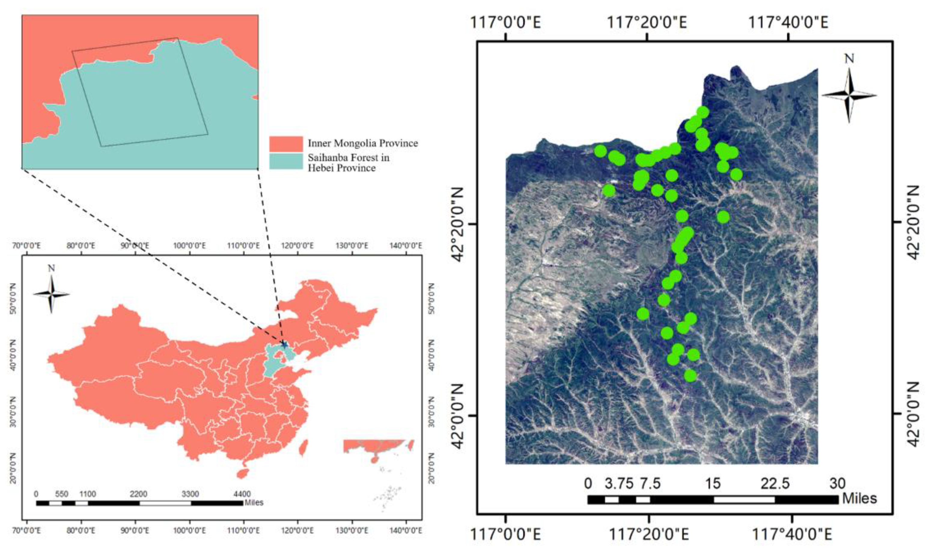
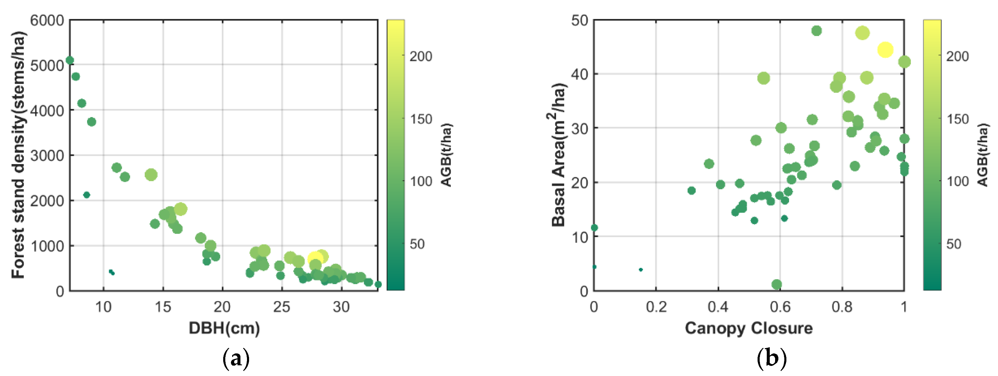
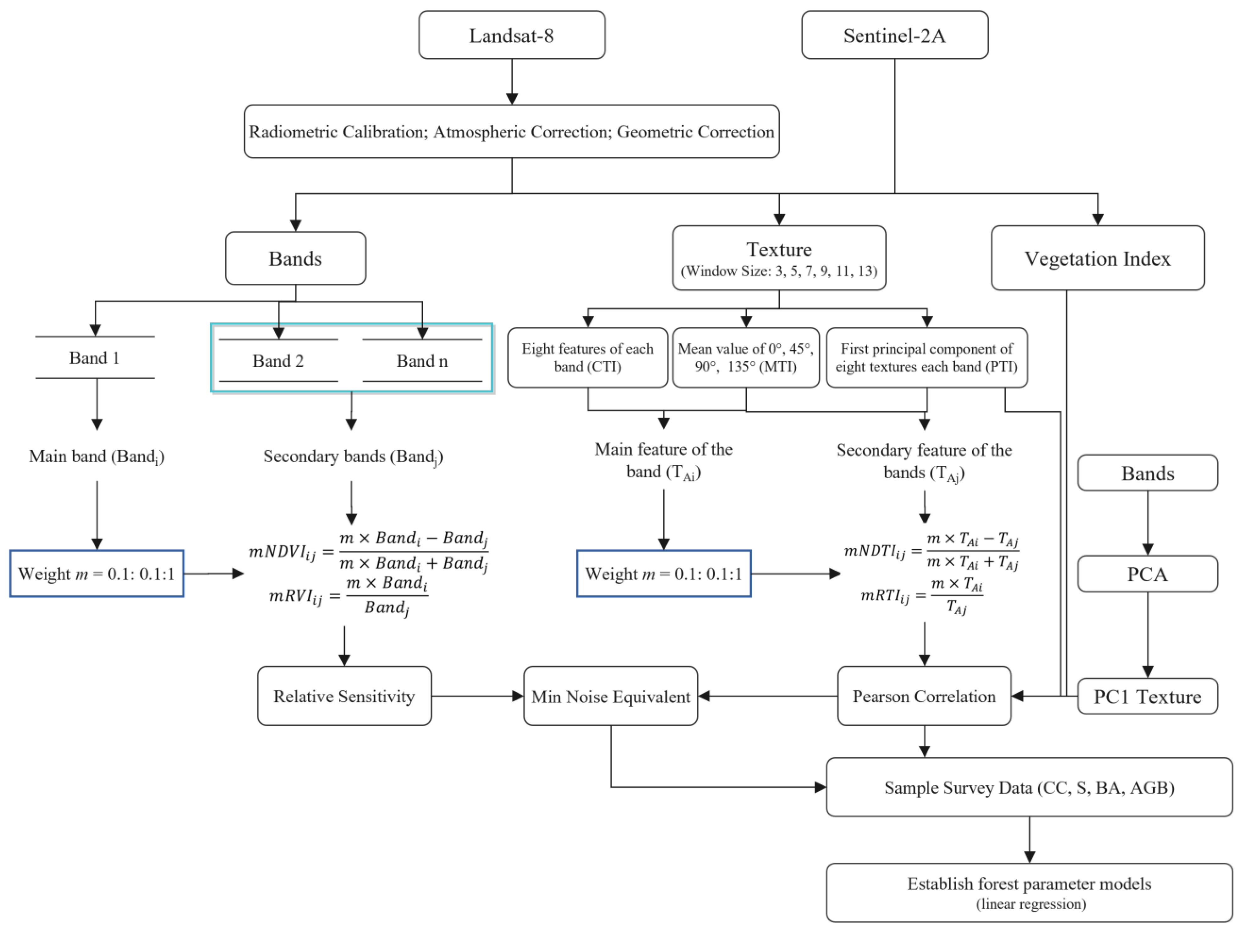
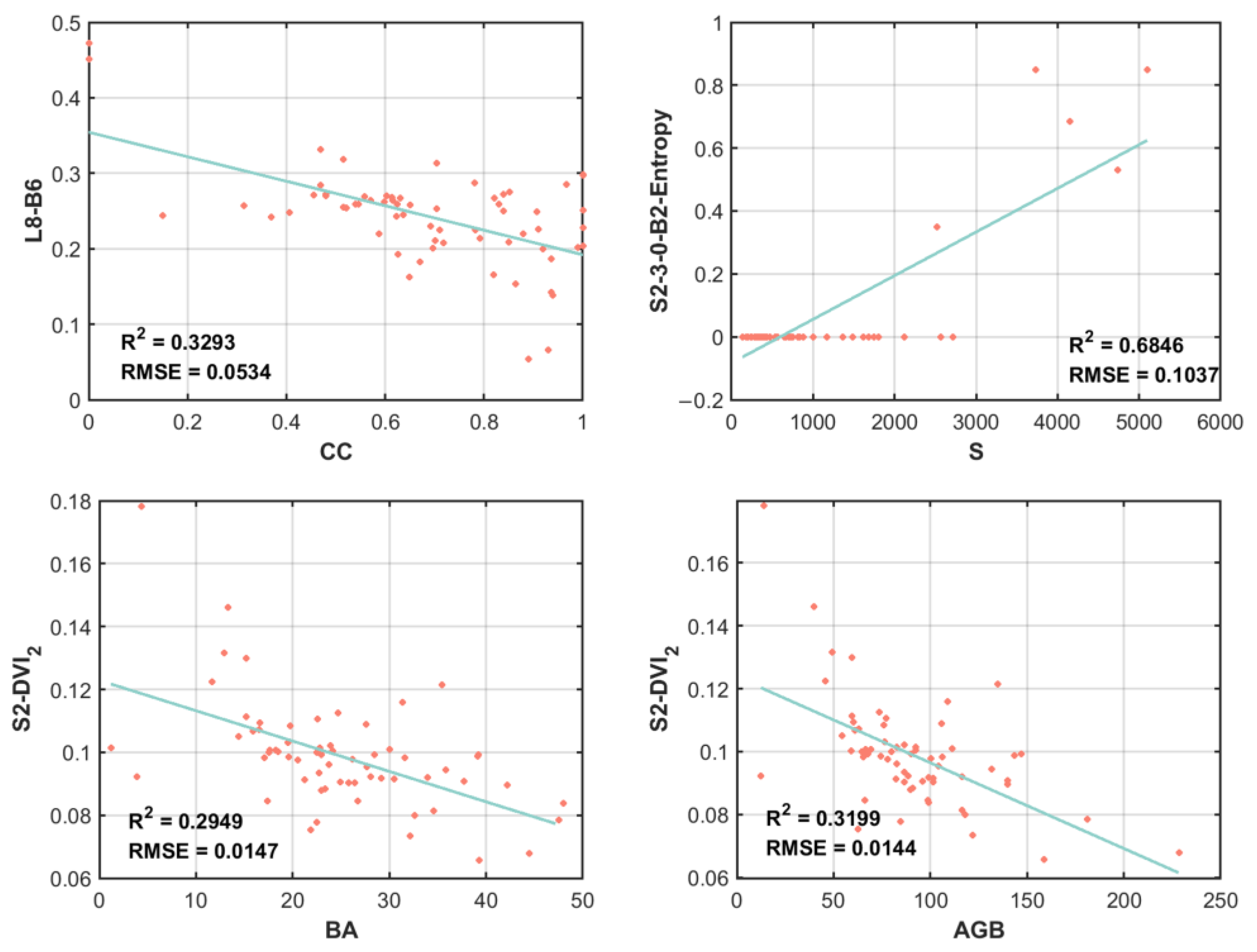
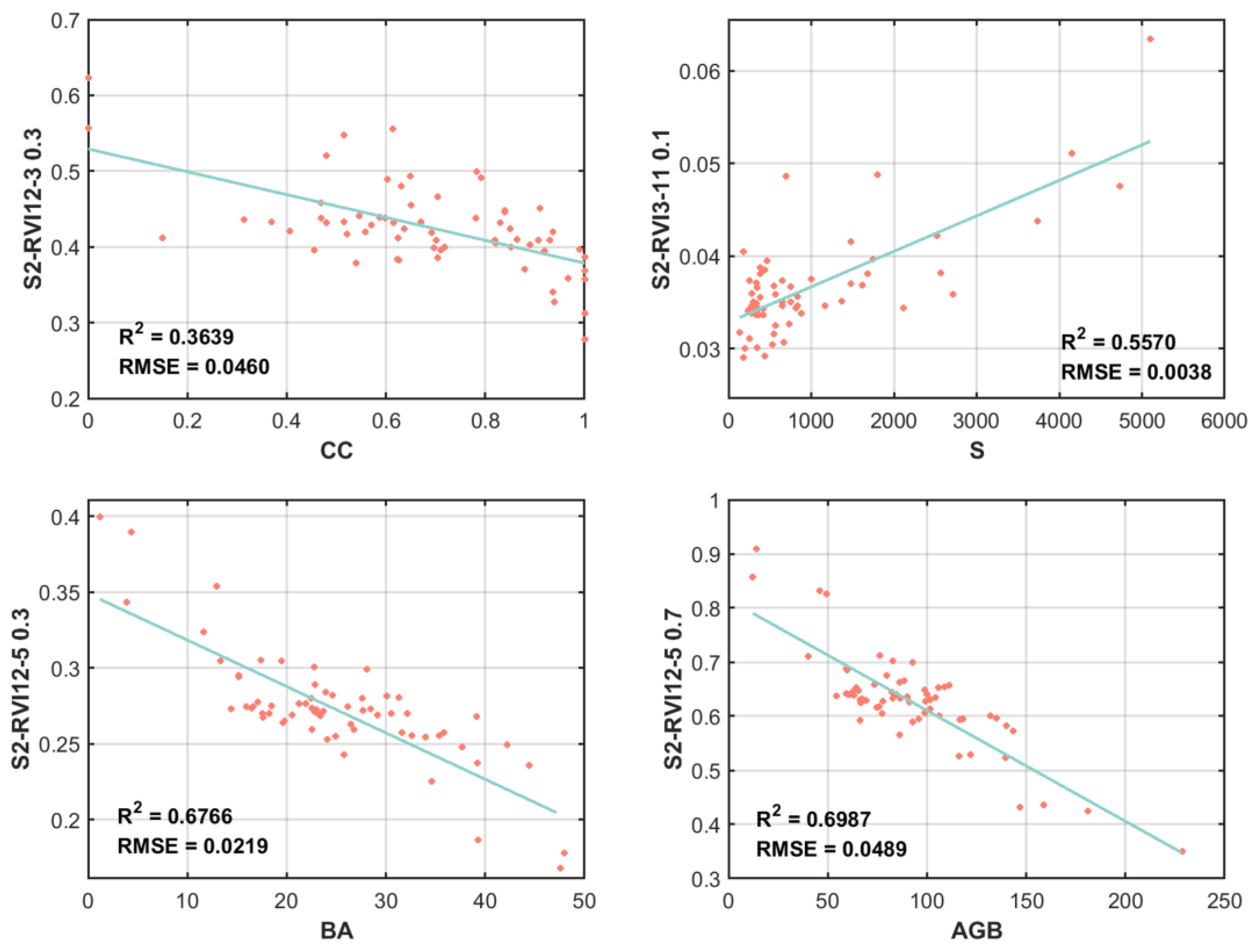
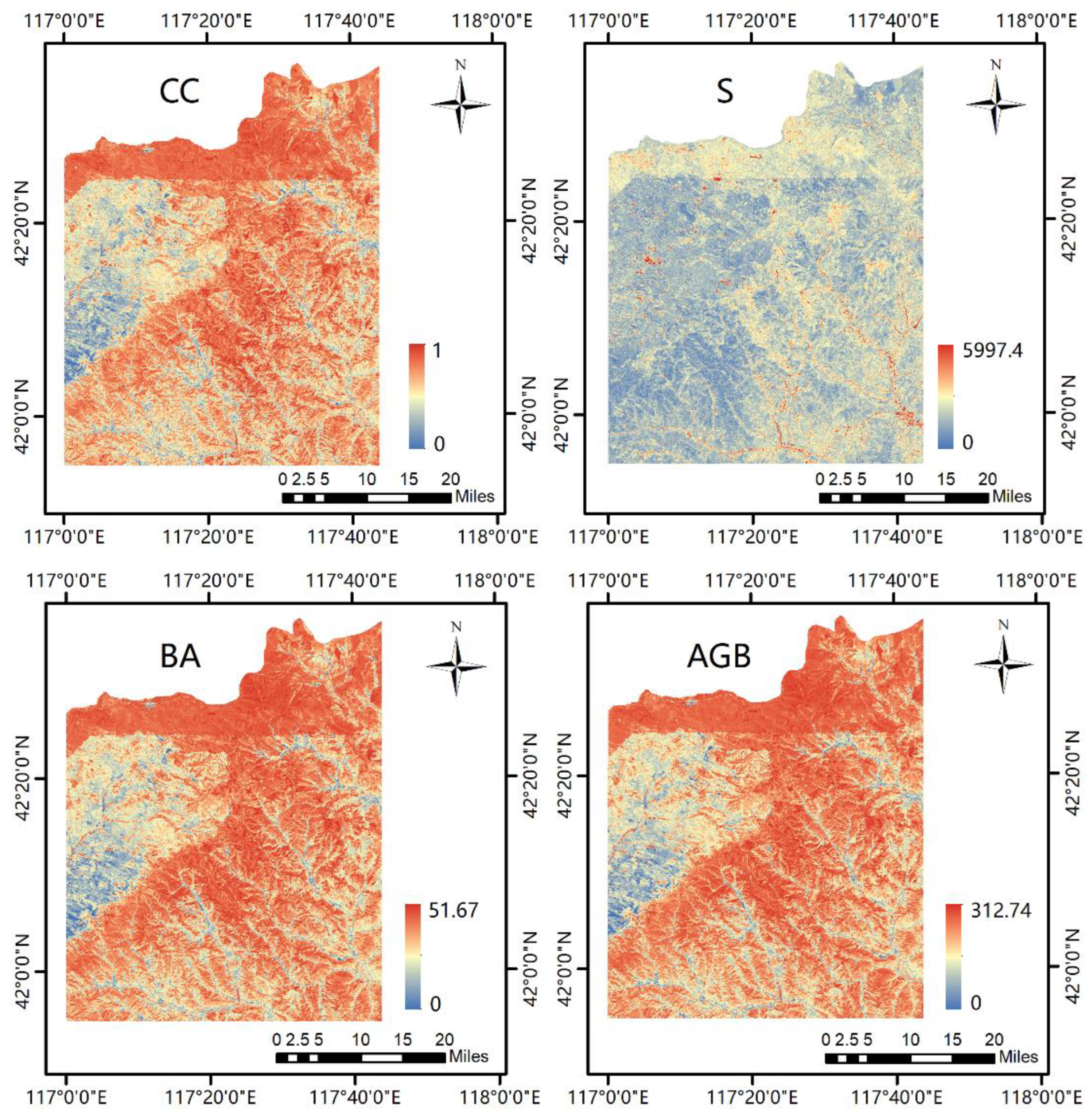
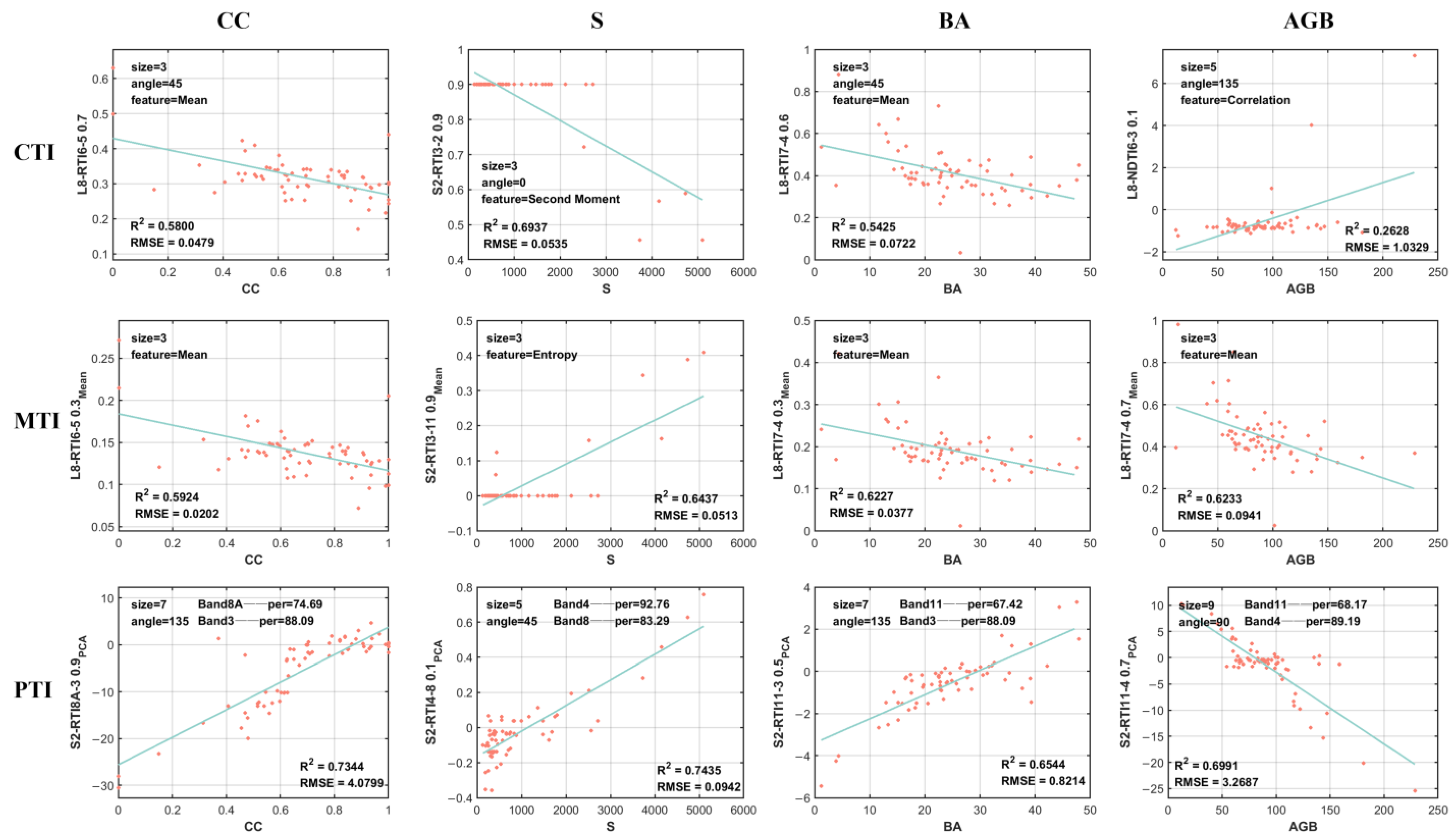
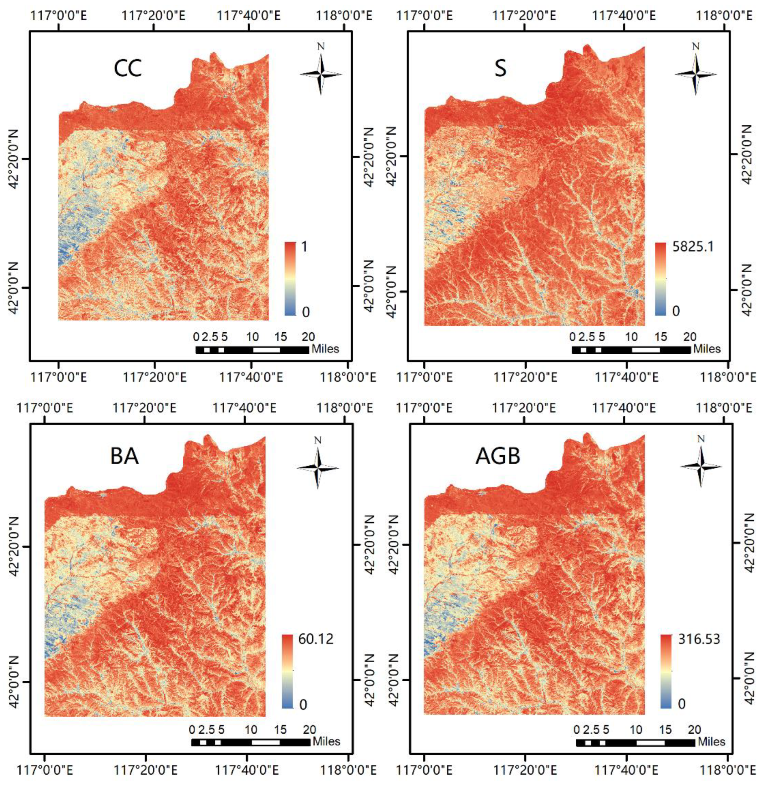
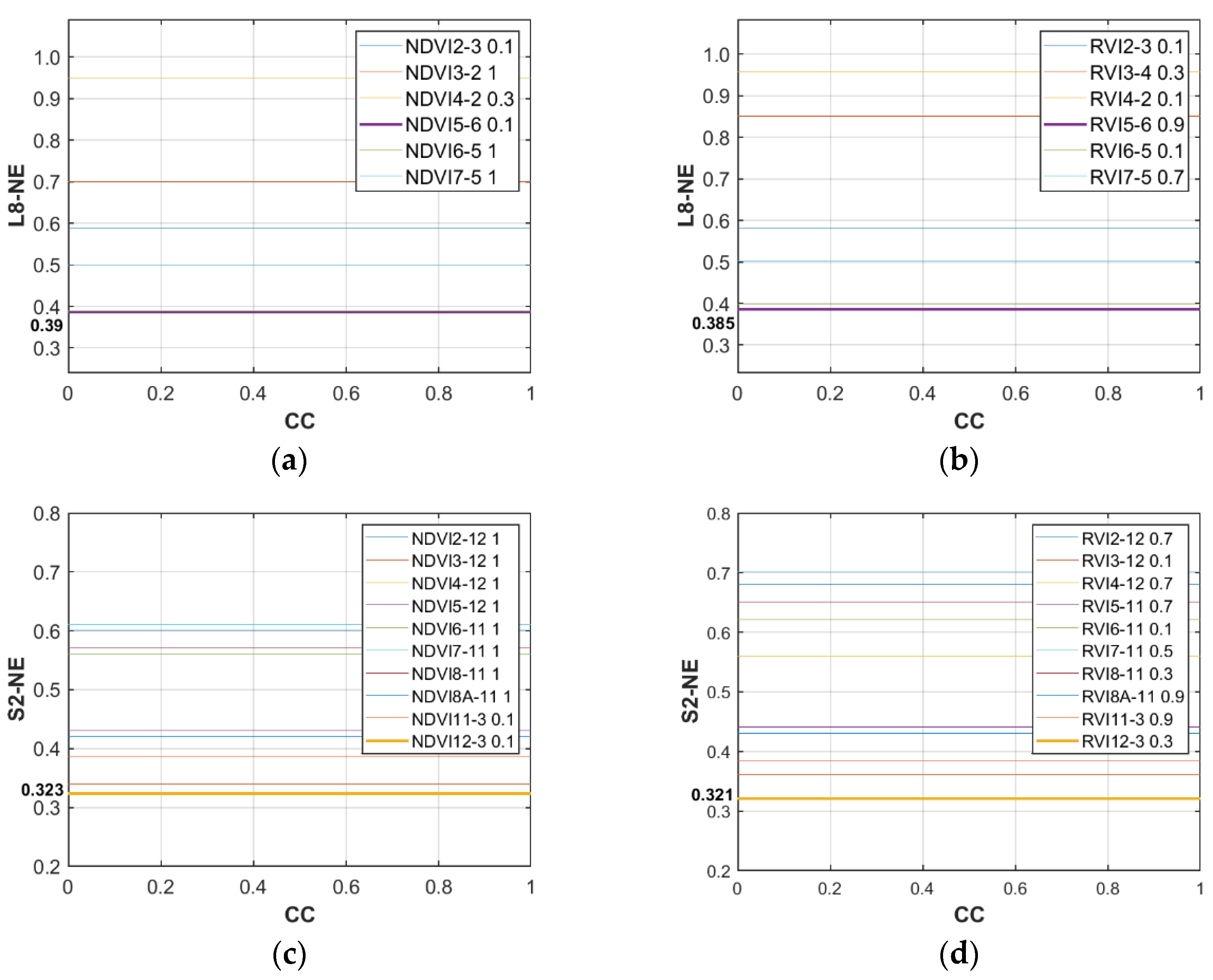
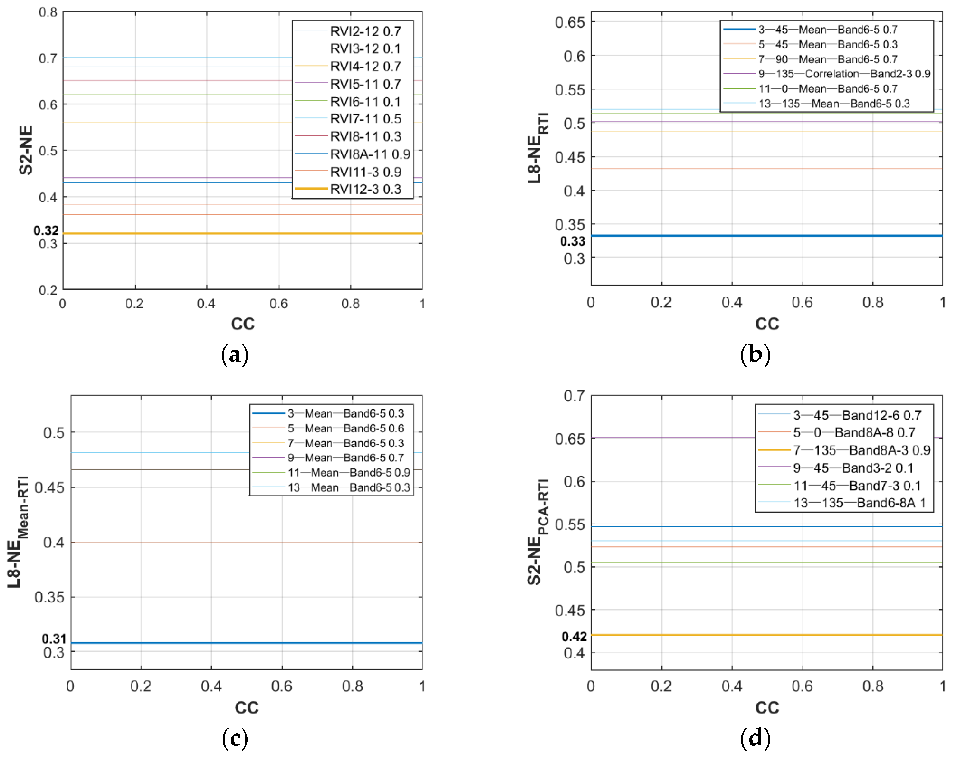
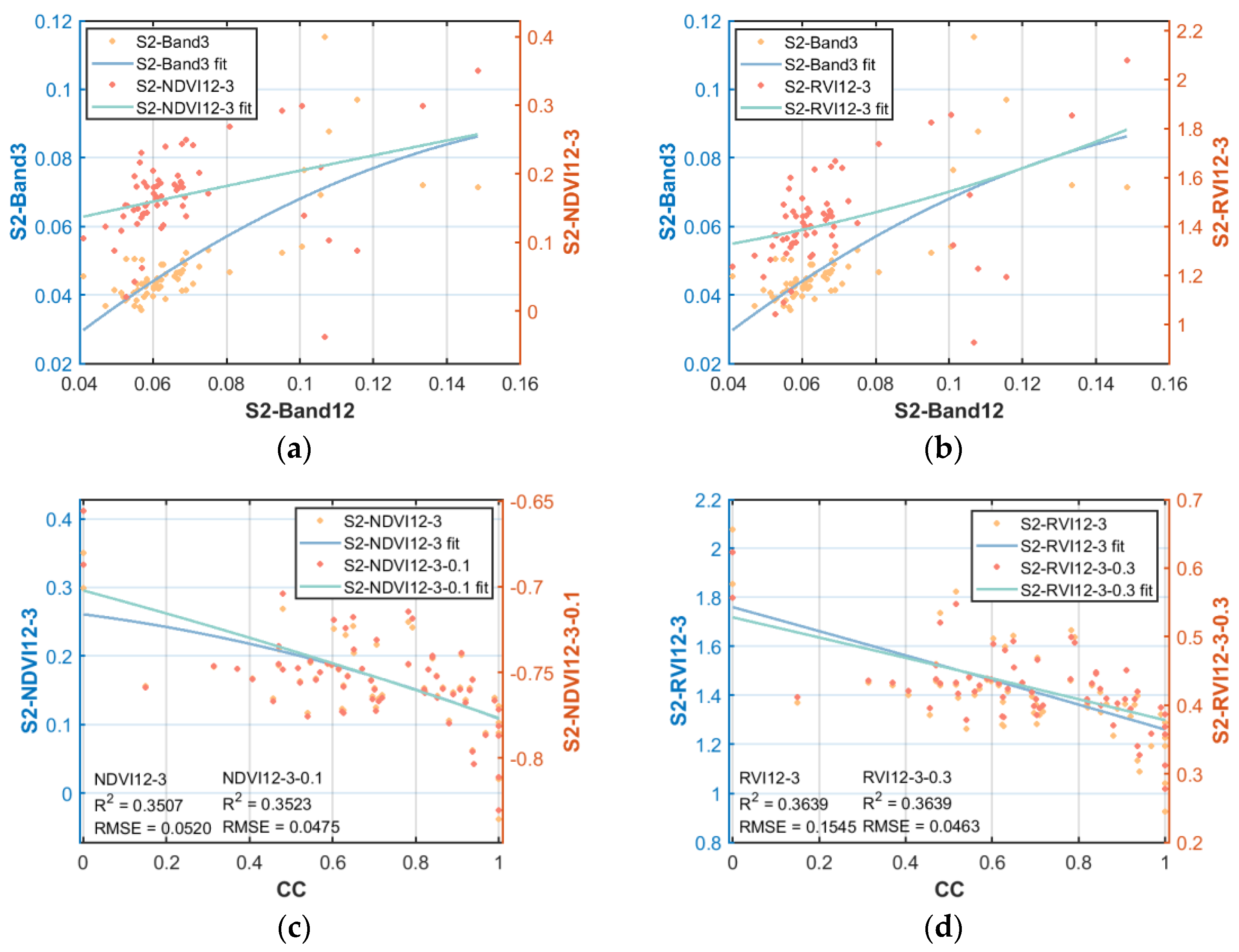
Table 1.
Summary of allometric growth equations for tree species in the sample site. The table shows the tree species recorded during the field work and the tree species allometric equations used to estimate biomass.
Table 1.
Summary of allometric growth equations for tree species in the sample site. The table shows the tree species recorded during the field work and the tree species allometric equations used to estimate biomass.
| Tree Species | Academic Name | Allometric Equation |
|---|---|---|
| Larch | Larix gmelinii (Rupr.) Kuzen. | AGB = 0.1431 [43] |
| Sphagnum pine | Pinus sylvestris var. mongholica Litv. | AGB = 0.093 [44] |
| Spruce | Picea asperata Mast. | AGB = 0.1199 [45] |
Table 2.
Sample plot information including maximum (Max), minimum (Min), mean, and standard deviation (STD) of mean DBH, CC, S, BA, and AGB.
Table 2.
Sample plot information including maximum (Max), minimum (Min), mean, and standard deviation (STD) of mean DBH, CC, S, BA, and AGB.
| Parameter | Max | Min | Mean | STD |
|---|---|---|---|---|
| Mean DBH (cm) | 33.1 | 7.2 | 22.74 | 7.33 |
| Canopy closure (%) | 1 | 0 | 0.69 | 0.23 |
| Forest stand density (stems/ha) | 5100 | 133.33 | 960.26 | 1083.45 |
| Basal Area (/ha) | 47.97 | 1.19 | 24.74 | 9.69 |
| AGB (t/ha) | 228.64 | 12.27 | 90.57 | 35.75 |
Table 3.
Correlation coefficients between forest parameters (mean DBH, CC, S, BA, and AGB) were measured and derived at the stand level.
Table 3.
Correlation coefficients between forest parameters (mean DBH, CC, S, BA, and AGB) were measured and derived at the stand level.
| Parameter | Pearson Correlation Coefficient | ||||
|---|---|---|---|---|---|
| Mean DBH | Canopy Closure | Forest Stand Density | Basal Area | AGB | |
| Mean DBH | 1 | - | - | - | - |
| Canopy closure | −0.333 | 1 | - | - | - |
| Forest stand density | −0.804 | 0.573 | 1 | - | - |
| Basal Area | −0.094 | 0.642 | 0.207 | 1 | - |
| AGB | 0.129 | 0.572 | 0.026 | 0.871 | 1 |
Table 4.
Table of optical data acquisition information.
| Sensor | Time | Spatial Resolution (m) |
|---|---|---|
| Landsat 8 | 16 June 2020 | 30 |
| Sentinel-2A | 21 June 2020 | 10, 20 |
Table 5.
The band information and the resolutions of S2A and L8 used in this paper.
| Sentinel-2A | Landsat 8 | |||||
|---|---|---|---|---|---|---|
| Band | Spectral Region | Resolution (M) | Spectral Region | Resolution (M) | ||
| Band2 | Blue | 0.46–0.52 | 10 | Blue | 0.45–0.51 | 30 |
| Band3 | Green | 0.54–0.58 | 10 | Green | 0.53–0.59 | 30 |
| Band4 | Red | 0.65–0.68 | 10 | Red | 0.64–0.67 | 30 |
| Band5 | Red edge1 | 0.70–0.71 | 20 | NIR | 0.85–0.88 | 30 |
| Band6 | Red edge2 | 0.73–0.75 | 20 | SWIR1 | 1.57–1.65 | 30 |
| Band7 | Red edge3 | 0.76–0.78 | 20 | SWIR2 | 2.11–2.29 | 30 |
| Band8 | NIR | 0.78–0.90 | 10 | |||
| Band8A | Narrow Near Infrared | 0.85–0.87 | 20 | |||
| Band11 | SWIR1 | 1.56–1.65 | 20 | |||
| Band12 | SWIR2 | 2.10–2.28 | 20 | |||
Table 6.
A summary table of the popular vegetation indices selected for this study, containing vegetation index formulas and references.
Table 6.
A summary table of the popular vegetation indices selected for this study, containing vegetation index formulas and references.
| Vegetation Index | Formula |
|---|---|
| Difference Vegetation Index [49] | |
| Enhanced Vegetation Index [50] | |
| Ratio Difference Vegetation Index [51] | |
| Soil Adjusted Vegetation Index [52] | |
| Optimization of Soil-Adjusted Vegetation Index [53] | |
| Atmospherically Resistant Vegetation Index [54] | |
| Infrared Percentage Vegetation Index [55] | |
| Modified Simple Ratio [56] | |
| Non-Linear Index [57] |
Table 7.
Equation of the GLCM texture metric.
| Texture [64] | Formula |
|---|---|
| Variance | |
| Homogeneity | |
| Contrast | |
| Dissimilarity | |
| Entropy | |
| Second Moment | |
| Correlation | |
| Mean |
Notes: is the element of the GLCM, which represents the probability of two gray values ( and ) with certain distance and direction. The sum of all values in GLCM is 1. N is the number of gray levels, i.e., the dimension of the GLCM [64].
Table 8.
Pearson correlation coefficients and between CC, S, BA, and AGB and variables derived from L8 and S2A data. The order of variables in the table are bands, vegetation indices, BTE, MTE, and PTE of L8 and S2A. Textures are defined and labeled using window_direction_band_texture features. Correlation is the correlation obtained by the Pearson method, and the value with ____ in the column is the optimal solution.
| Parameter | Sensor | Variables | Correlation | R2 |
|---|---|---|---|---|
| CC | L8 | B6 | −0.57 *** | 0.3293 |
| S2A | −0.54 *** | 0.3156 | ||
| L8 | BTE_3_0_B6_mean | −0.47 *** | 0.2214 | |
| L8 | MTE_3_B6_mean | −0.45 *** | 0.2020 | |
| L8 | PTE_13_90_correlation | 0.35 ** | 0.1192 | |
| S | S2A | B3 | 0.74 *** | 0.5472 |
| S2A | −0.4 *** | 0.4003 | ||
| S2A | BTE_3_0_B2_entropy | 0.83 *** | 0.6846 | |
| S2A | MTE_3_B2_homogeneity | −0.8 *** | 0.6360 | |
| S2A | PTE_13_0_correlation | −0.55 *** | 0.2974 | |
| BA | S2A | B11 | 0.48 *** | 0.2312 |
| S2A | DVI2 | −0.48 *** | 0.2949 | |
| S2A | BTE_3_0_B11_mean | −0.48 *** | 0.2339 | |
| S2A | MTE_3_B11_mean | −0.46 *** | 0.2109 | |
| L8 | PTE_13_45_correlation | 0.47 *** | 0.2189 | |
| AGB | S2A | B11 | −0.55 *** | 0.3054 |
| S2A | DVI2 | −0.46 *** | 0.3199 | |
| S2A | BTE_3_0_B11_mean | −0.52 *** | 0.2755 | |
| S2A | MTE_5_B11_mean | −0.45 *** | 0.1984 | |
| L8 | PTE_11_45_correlation | 0.45 *** | 0.2004 |
*** Correlation is significant at the 0.001 level. ** Correlation is significant at the 0.01 level.
Table 9.
Summary of the results of the optimal vegetation indices obtained using screening different sensors after adding weights to the bands.
Table 9.
Summary of the results of the optimal vegetation indices obtained using screening different sensors after adding weights to the bands.
| Parameter | Sensor | BAND_VI | RMSE | ||
|---|---|---|---|---|---|
| CC | S2A | RVI12-3 | 0.3 | 0.3639 | 0.0460 |
| S | S2A | RVI3-11 | 0.1 | 0.5570 | 0.0038 |
| BA | S2A | RVI12-5 | 0.3 | 0.6766 | 0.0219 |
| AGB | S2A | RVI12-5 | 0.7 | 0.6987 | 0.0489 |
Table 10.
Summary table of optimal CTI results.
| Parameter | Sensor | BAND_TI | Size | Angle | Feature | RMSE | ||
|---|---|---|---|---|---|---|---|---|
| CC | L8 | RTI6-5 | 0.7 | 3 | 45 | Mean | 0.5800 | 0.0479 |
| S | S2A | RTI3-2 | 0.9 | 3 | 0 | Second Moment | 0.6937 | 0.0535 |
| BA | L8 | RTI7-4 | 0.6 | 3 | 45 | Mean | 0.5425 | 0.0722 |
| AGB | L8 | NDTI6-3 | 0.1 | 5 | 135 | Correlation | 0.2628 | 1.0329 |
Table 11.
Summary table of optimal MTI results.
| Parameter | Sensor | BAND_TI | Size | Feature | RMSE | ||
|---|---|---|---|---|---|---|---|
| CC | L8 | RTI6-5 | 0.3 | 3 | Mean | 0.5924 | 0.0202 |
| S | S2A | RTI3-11 | 0.9 | 3 | Entropy | 0.6437 | 0.0513 |
| BA | L8 | RTI7-4 | 0.3 | 3 | Mean | 0.6227 | 0.0377 |
| AGB | L8 | RTI7-4 | 0.7 | 3 | Mean | 0.6233 | 0.0941 |
Table 12.
Summary of the results of the optimal PTIs. Per1 and Per2 contain the amount of information after principal component analysis for the main and secondary texture features, respectively.
Table 12.
Summary of the results of the optimal PTIs. Per1 and Per2 contain the amount of information after principal component analysis for the main and secondary texture features, respectively.
| Parameter | Sensor | BAND_TI | Size | Angle | RMSE | ||||
|---|---|---|---|---|---|---|---|---|---|
| CC | S2A | RTI8A-3 | 0.9 | 7 | 135 | 74.6949 | 88.0945 | 0.7344 | 4.0799 |
| S | S2A | RTI4-8 | 0.1 | 5 | 45 | 92.7594 | 83.2894 | 0.7435 | 0.0942 |
| BA | S2A | RTI11-3 | 0.5 | 7 | 135 | 67.4230 | 88.0945 | 0.6544 | 0.8214 |
| AGB | S2A | RTI11-4 | 0.7 | 9 | 90 | 68.1722 | 89.1878 | 0.6991 | 3.2687 |
Table 13.
Summary table of optimal results for each index obtained using CC.
| Parameter | Index | Sensor | BAND | RMSE | ||
|---|---|---|---|---|---|---|
| CC | VI | S2A | RVI12-3 | 0.3 | 0.3639 | 0.0460 |
| CTI | L8 | RTI6-5 | 0.7 | 0.5800 | 0.0479 | |
| MTI | L8 | RTI6-5 | 0.3 | 0.5924 | 0.0202 | |
| PTI | S2A | RTI8A-3 | 0.9 | 0.7344 | 4.0799 |
Disclaimer/Publisher’s Note: The statements, opinions and data contained in all publications are solely those of the individual author(s) and contributor(s) and not of MDPI and/or the editor(s). MDPI and/or the editor(s) disclaim responsibility for any injury to people or property resulting from any ideas, methods, instructions or products referred to in the content. |
© 2023 by the authors. Licensee MDPI, Basel, Switzerland. This article is an open access article distributed under the terms and conditions of the Creative Commons Attribution (CC BY) license (https://creativecommons.org/licenses/by/4.0/).
Share and Cite
MDPI and ACS Style
Sa, R.; Fan, W. Estimation of Forest Parameters in Boreal Artificial Coniferous Forests Using Landsat 8 and Sentinel-2A. Remote Sens. 2023, 15, 3605. https://doi.org/10.3390/rs15143605
AMA Style
Sa R, Fan W. Estimation of Forest Parameters in Boreal Artificial Coniferous Forests Using Landsat 8 and Sentinel-2A. Remote Sensing. 2023; 15(14):3605. https://doi.org/10.3390/rs15143605
Chicago/Turabian StyleSa, Rula, and Wenyi Fan. 2023. "Estimation of Forest Parameters in Boreal Artificial Coniferous Forests Using Landsat 8 and Sentinel-2A" Remote Sensing 15, no. 14: 3605. https://doi.org/10.3390/rs15143605
Note that from the first issue of 2016, this journal uses article numbers instead of page numbers. See further details here.