
Recent Advances and Challenges in Schumann Resonance Observations and Research
by
 , ,
, ,
Jinlai Liu
1,2 ,
,
Jianping Huang
1,2,3,*,
Zhong Li
3,
Zhengyu Zhao
4,
Zhima Zeren
2,
Xuhui Shen
5 and
Qiao Wang
2 1
School of Emergency Management Science and Engineering, University of Chinese Academy of Sciences, Beijing 100049, China
2
National Institute of Natural Hazards, Ministry of Emergency Management of China, Beijing 100085, China
3
School of Information Engineering, Institute of Disaster Prevention, Langfang 065201, China
4
School of Electronic Information, Wuhan University, Wuhan 430072, China
5
State Key Laboratory of Space Weather, National Space Science Center, Chinese Academy of Sciences, Beijing 100190, China
*
Author to whom correspondence should be addressed.
Remote Sens. 2023, 15(14), 3557; https://doi.org/10.3390/rs15143557
Submission received: 15 April 2023
/
Revised: 20 June 2023
/
Accepted: 12 July 2023
/
Published: 15 July 2023
(This article belongs to the Section Remote Sensing and Geo-Spatial Science)
Abstract
:The theoretical development of Schumann Resonances has spanned more than a century as a form of global natural electromagnetic resonances. In recent years, with the development of electromagnetic detection technology and the improvement in digital processing capabilities, the connection between Schumann Resonances and natural phenomena, such as lightning, earthquakes, and Earth’s climate, has been experimentally and theoretically demonstrated. This article is a review of the relevant literature on Schumann Resonance observation experiments, theoretical research over the years, and a prospect based on space-based observations. We start with the theoretical background and the main content on Schumann Resonances. Then, observations and the identification of Schumann Resonance signals based on ground and satellite data are introduced. The research and related applications of Schumann Resonances signals are summarized in terms of lightning, earthquakes, and atmosphere. Finally, the paper presents a brief study of Schumann Resonances based on the China Seismo-Electromagnetic Satellite (CSES) and preliminary ideas about how to improve the identification and application of space-based Schumann Resonances signals.
1. Introduction
The Earth–ionosphere cavity is composed of the Earth’s surface with high conductivity, the conductive but dissipative ionosphere, and an insulating air layer in the middle. The cavity formed between the Earth’s surface and the ionosphere allows for the presence of quasi-electromagnetic standing waves, whose wavelengths are comparable to that of interplanetary waves [1]. In the lower atmosphere, up to 60–70 km above the Earth’s surface, the limited electrical conductivity of the atmosphere is mainly maintained by cosmic rays [2]. Near the ground, the conductivity is around the order of 10–14 S/m, thus making this area a good electrical insulator. The conductivity increases exponentially with height on a characteristic scale of 3–6 km, from the ground to 75–95 km below the E layer, and its specific value depends on local time and height. Above this height, the ratio of the electron cyclotron frequency to the electron-neutral particle’s collision frequency cannot be ignored, and the conductivity becomes a tensor [3,4]. In the upper part of the D layer and the lower part of the E layer, the conductivity component parallel to the magnetic field is about 10−4~10−2 S/m, which can be compared with the conductivity magnitude of the Earth’s surface and water. For ELF waves (3–300 Hz), the transmission between the insulated lower atmosphere and the ionosphere occurs at 40–50 km [5]. For the lower atmosphere, the main effect is electron displacement, while for the ionosphere, conduction is the major influence [6].
Some strong electrical transient processes, such as lightning and electromagnetic radiation pulses, extend from the excitation source into the cavity. This process was studied by many scientists through experimental simulations of conducting concentric spheres in the late 18th and early 19th centuries. In 1893, George Francis Fitz Gerald [7] first proposed the hypothesis of Earth’s natural electromagnetic resonance based on the early concentric conductive sphere experiment and the atmospheric conductive layer hypothesis at that time. In 1894, Joseph Larmor [8] calculated and derived the formula for the free period in a uniform spherical capacitor, which was identical to the formula derived by Schumann in 1952 but was not applied to the Earth–ionosphere cavity at that time. In 1921, Charles T.R. Wilson [9] proposed the concept of a global atmospheric circuit, where positive charges are transmitted through conduction to the upper atmosphere of the Earth’s surface and ionosphere to form a discharge current, while negative charges are transmitted to the Earth’s surface through cloud to ground lightning strikes to generate a charging current. The concept of global atmospheric circuits has rapidly promoted research on Earth–ionosphere waveguides and SR-lightning field sources. For example, Schelkunoff, Rydbeck, and others [10,11] studied the wave propagation problem of concentric conductive spheres and deduced the wave function and resonance frequency equation between concentric conductive spheres, but they did not clearly calculate the solution of the equation, nor connect the conclusion with Earth–ionosphere waveguides. The above research approached the core of the Schumann Resonance (SR) phenomenon, providing experimental and theoretical support for the later establishment of SR theory.
In 1952, Winfried Otto Schumann [12,13] deduced the formula of the characteristic frequency of the Earth–ionosphere cavity and pointed out that SR propagates in the narrow dielectric interface between the surface and the ionosphere, and the height of the interface is far less than the Earth’s radius. From 1952 to 1957, Schumann [14,15,16,17,18,19] proposed the resonance theory of ELF waves excited by lightning discharge in the Earth–air–ionosphere system waveguide. His theory consists of three main parts: (1) electromagnetic wave propagation in a spherical cavity, (2) the Earth–air–ionosphere system as a waveguide, and (3) lightning discharge as an excitation source. The ELF (extremely low-frequency) resonance theory was first published by Schumann and named by Charles Polk after him [20], which is now called SR.
SR is a natural electromagnetic resonance phenomenon, which is mainly excited naturally by global lightning discharges and propagates by oscillations back and forth in the Earth–ionosphere cavity. The lowest frequency component of electromagnetic impulse (thunderstorms and high-altitude explosions, etc.) can orbit the Earth several times before undergoing decay. During the process, phase increase and wave cancellation generate a resonance spectrum, where wave cancellations always follow multiple paths [21,22]. The main characteristics of this resonance spectrum can be explained by the quasi TEM wave theory, where all resonance spectra are not correlated with the superposition of the global thunderstorm effect [23]. SR can be observed in many different places and can be detected anywhere in interstellar space. The strength of the electrical and magnetic components of SR is very weak, and it is easily mixed with nearby lightning and a large amount of unrelated human electromagnetic noise. However, in addition to lightning and artificial electromagnetic noise sources, SR is an important component of the natural background electromagnetic noise spectrum from 5 to 50 Hz [1]. For the SR effect, a more general approach is to study the propagation of ELF waves.
Madden and Thompson [24] made a great contribution to ELF wave propagation theoretical models in the 1960s. First, they pointed out that the main dissipation of SR transmission occurs in the D region of the low ionosphere, and considered the problem of leakage in the Earth–ionosphere cavity (limited to nighttime) for the first time. In studying the impact of nuclear explosions on ionospheric disturbances, an equivalent circuit model was designed to attempt to solve the SR problem. The dissipation problem of SR/ELF waves was later independently studied by Greifinger et al. [25]. Greifinger et al. derived an approximate expression for the TEM eigenvalues of ELF waves propagating in the Earth’s ionospheric waveguide, ignoring the anisotropy caused by the Earth’s magnetic field. Greifinger also indicated that the eigenvalues are mainly determined by the properties of the ionosphere near the two clear heights where the maximum Ohmic dissipation occurs. Mushtuk and Williams [26] proposed a knee model for simulating a uniform earth–ionosphere waveguide based on Greifinger et al. that could accurately simulate experimental observations within the SR frequency range; the model showed that as the SR frequency increases, the Q factor also increases. The knee model mainly considers the transition from ion-dominated to electron-dominated conductivity in the lower characteristic layer of the ionosphere. Williams, Mushtak, and Nickolaenko et al. [27] compared five uniform cavity models with significant differences in waveguide dissipation behavior, and pointed out that the Lorentz process is suitable for estimating the adequacy level of these propagation parameter models, and that the knee model variables have a statistically significant and physically consistent contrast between the estimated solar activity minima and solar activity maxima for the upper magnetic layer.
The transmission and dissipation processes of SR are different during the day and nighttime. Due to the need for studying the asymmetry of day and night, Pechony and Zhou H et al. [28,29] used a non-uniform empirical “knee” model for distinguishing day and night based on the classic “knee” model. Madden and Thompson [24] provided information on the energy dissipation of EM waves in the first SR frequency band of the ionosphere with altitude variations in mid-latitude daytime and night states as early as 1965. In a cavity with day–night asymmetry, assuming that the termination line passes through the two poles and splits the Earth into two equal hemispheres, the conductivity suddenly changes at the boundary between the day–night hemispheres without any tilt, which is sufficient to evaluate the relative impact of day–night asymmetry and source migration on SR parameters.
The determination of basic theories has rapidly promoted the progress of SR research. It is now widely believed that intra-cloud lightning and cloud-to-ground lightning release is the primary source of SR, with a global average thunderstorm rate of 100/S. The peak energy released by it reaches 20,000–30,000A, with an average distance of 3–5 km, which is sufficient to observe SR for exciting the Earth–ionosphere cavity. Lightning discharges, the primary natural source of SR, occur primarily in three areas of global thunderstorm activity, including South America, Africa, and Southeast Asia [30,31]. In addition, local dense lightning can also excite SR. Simultaneous observation of SR anomalies in France, Italy, Russia, and Japan were reported during the 2022 Tonga eruption, where localized lightning field sources were formed by aggregation in the eruption cloud [32]. J. Bor et al. [33] used the data observed by multiple SR and PG (potential gradient) measurement stations distributed globally to study the GEC’s response to the eruption of the Tonga volcano. SR and PG intensities were used to describe the AC (alternating current) and DC (direct current) components of the GEC, respectively. The SR measurements indicated that the impact of lightning activity in the eruption is global. The DC component of the GEC was charged twice during the eruption by cloud-to-ground lightning strikes. Nickolaenko et al. [34] used the vertical electric field and two orthogonal horizontal magnetic field components recorded from multi-station SR observations to calculate the Umov–Poynting vector (UPV), which can be used to locate and estimate eruptive activity. During the eruption of the Tonga volcano, charged dust and dust plasma may have discharged during charge accumulation, forming local lightning sources under certain circumstances, which in turn excite SR, but have no significant effect on real global thunderstorm activity [35,36]. Analyzing the geomagnetic field disturbance and SR response during the 2022 Tonga eruption, Gavrilov et al. [37] concluded that Tonga volcanic activity generates global geomagnetic disturbances via acoustic–gravity waves (AGW), which leads to changes in ionospheric conductivity, ionospheric current values, and the geomagnetic field; the analysis also revealed that SR signal properties are related to the number and energy of lightning discharges. Qiaoli Kong et al. [38] studied vertical ionospheric disturbance types during volcanic activity and classified the origins of the disturbances as acoustic–gravity wave, Lamb wave, and tsunami wave.
When lightning activity occurs, the lightning channel is similar to a huge electromagnetic wave transmitting antenna, emitting electromagnetic energy with a radiation frequency below 100 kHz. Although lightning signals below 100 Hz are very weak, their attenuation is only 0.5 dB/mm, so the electromagnetic waves generated by a single lightning activity discharge can propagate multiple times globally and then attenuate into background noise [39]. When the wavelength of the ELF wave is equivalent to the circumference of the Earth (about 4000 km), electromagnetic waves propagating in the opposite direction in the Earth–ionosphere cavity interfere with the straight beam excited by lightning at the SR frequency, amplifying the spectral signal from lightning and ultimately leading to the appearance of harmonic peaks of various modes of SR in the ELF spectrum.
SR signals propagate within the Earth–ionosphere cavity, where the cavity between the Earth and the ionosphere can be seen as a waveguide with infinite horizontal width but limited vertical depth. For cavities with ideal conductive boundaries, the SR eigenfrequency is approximately given by the average radius a of the resonant cavity and the speed of light (Equation (1)).
By substituting the specific value of n, the SR frequency without loss can be obtained: Hz, Hz, Hz, etc. The SR eigenmodes based on digital simulation also showed the same results [40].
Due to the resonance effect, SR mainly propagates in a transverse magnetic field (TM) mode within the cavity, with significantly higher transmission energy than other frequencies [41]. The loss of electromagnetic waves in the real Earth–ionospheric cavity medium is mainly propagated in the D region of the low ionosphere at the system boundary. The loss in the medium of the real Earth–ionosphere cavity leads to a broadening of the resonance lines and lowering of the resonance peak frequencies in comparison with the “ideal case” [42].
2. Observation Methods
2.1. Ground Observation
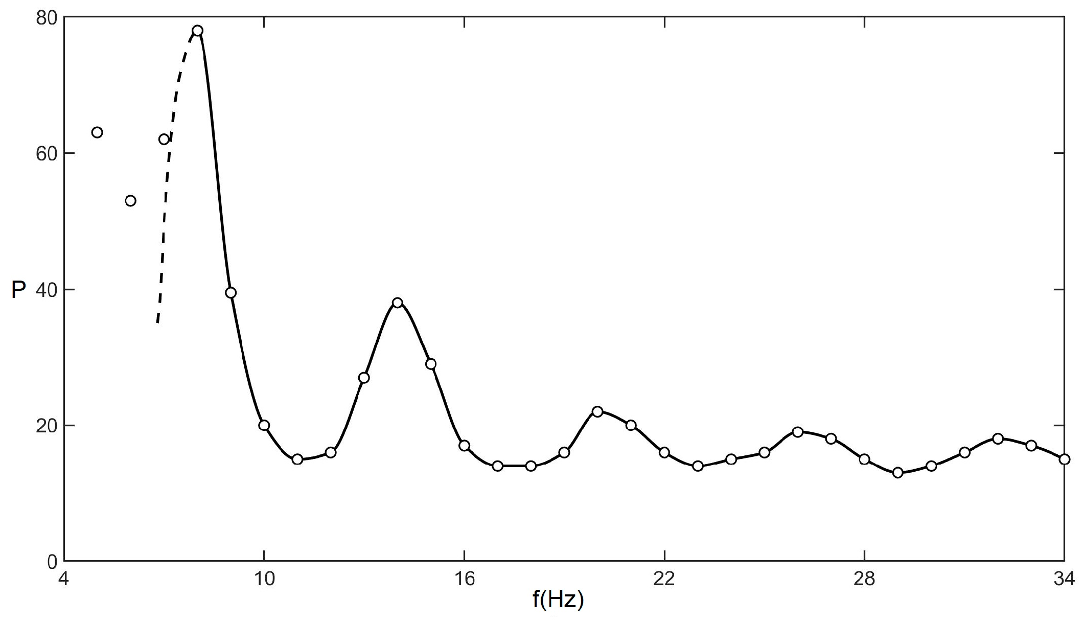
Ground-based observation has always been a common method for obtaining SR electromagnetic data and conducting related research. In 1960, Martin Balser and Charles A. Wagner [43] first published ground-based observations characterizing the first five eigenmodes of SR, as shown in Figure 1.
With the popularization of radio technology and the rapid development of software and hardware, relevant research teams have been designing and manufacturing receiving systems for SR-related research. For example, Ohta et al. designed a ULF/ELF observation system that utilizes narrowband sensors to receive signals within the SR frequency band [44]. The sensor’s signal records can display characteristics that are not present in amplitude changes generated by broadband sensors, which is conducive to real-time monitoring of SR anomalies before earthquakes.
In recent years, with the development of technology, devices used to collect SR signals have gradually become portable and diverse. Votis et al. [45] independently designed a portable SR receiver and received stable SR signals over a continuous period of time. Cano Domingo [46] added a sensor with the average center frequency of the first eigenmode of SR as the focus in the portable acquisition device to broaden the system response to extract transient events with a higher resolution. Tatsis et al. [47] designed a prototype testing fixture for calibrating SR measurement equipment to test the accuracy and stability of SR antenna receivers. In addition, the background of SR is also shown in the gravitational wave measurement results of the interferometer [48,49]. During the period of China’s tenth five-year plan, China established the “China Digital Seismic Observation Network” project, in which 12 very low-frequency observatories continuously observe the natural electromagnetic field from 0.1 to 800 Hz according to a unified specification, providing important data support for ELF signal propagation and seismic-prediction-related research [50].
ELF electromagnetic data processing and SR extraction and analysis methods have also developed rapidly. Based on the nonlinear interaction model between SR signals and HF electromagnetic waves under the action of atmospheric electric fields, Cao B.X. et al. [51] used the first batch of SR observation stations in China to obtain the SR spectrum through short-wave timing signal BPM demodulation. Rodríguez Camacho et al. [52] determined the amplitude spectrum from the measured low-amplitude noise signal and manually denoised it. Finally, they calculated the analysis function to fit the filtered amplitude spectrum and extracted accurate SR parameters. Soler Ortiz [53] proposed a new method for statistical analysis of SR signals in the time domain. By using the maximum likelihood parameter estimation and distribution fitting of the Akaike Information Criterion (AIC), statistical analysis is applied to characterize the time series of SR and the bandwidth of their ELF spectrum. Salinas et al. [54] combined the Lorentz function and linear term to perform nonlinear fitting on the measured ELF spectrum to identify the existence of SR and quantitatively characterize it. They used the Levenberg–Marquad algorithm to optimally constrain the measured SRs and extract the SR parameters with high confidence.
2.2. Satellite Observation
Compared with ground observation, increasing the observation height is beneficial for receiving more abundant electromagnetic information. In 1977, T. Ogawa [55] observed the first seven eigenmodes of SR signals at stratospheric altitude using high-altitude balloons. With the development of space technology, satellite payloads are more sensitive and precise, and electromagnetic satellite monitoring has gradually become the main means of space-physics-related research. Zhao Z.Y. et al. [56] used the ELF electromagnetic observation data of Aureol-3 near Earth’s polar orbit low-altitude satellite on ionospheric electric field disturbance and electron density disturbance at the height of ionosphere layer F, observed SR signals in the electric field component and showed that the SR eigenfrequency occurring in the upper ionosphere is related to the large-scale irregularity and positive density gradient of electron density, which is the first SR research based on satellite data. Later, Ni B.B. and Zhao Z.Y. [41] pointed out that the electric field component observed by the Aureol-3 satellite has a good resonance spectral structure, and the peak frequency corresponds to the various SR eigenfrequencies in the magnetic field component, confirming that the ELF wave field disturbance observed by the Aureol-3 satellite is an electromagnetic oscillation related to SR. In 2011, Simões et al. [57] detected and extracted SR signals at the ionosphere F-layer height using electric field data collected by the C/NOFS satellite during abnormally low solar activity minima. The C/NOFS satellite observes ionospheric electromagnetic signals at the height of the ionosphere F-layer, and can observe significant SR phenomena under nighttime conditions. In 2014, Dudkin et al. [58] extracted characteristic records of ionospheric Alfven resonance and SR using the ULF/ELF electric field observation data of the Chibis-M satellite. Simões and Dudkin [57,58] extracted SR signals based on satellite altitude observations, which proved the spatial SR leakage mentioned by Madden and Thompson [24]. Toledo Redondo et al. [59] used more than four years of electric field data sets from the DEMETER satellite to produce detailed maps of the effective ionospheric reflection height or D-region height, which is inversely proportional to the cutoff frequency. The depiction of the Toledo-Redondo et al. map ranges within 60° north–south latitudes, while the global SR background field based on CSES is within 65° north–south latitudes. The SR background and Toledo-Redondo’s maps both apparently shows anomalous enhancement due to geographic and geomagnetic misalignments. Toledo’s research can support subsequent studies of SR context based on satellite data.
3. Schumann Resonance and Lightning
SR is closely related to global lightning and can provide useful information about global thunderstorm activity and low ionospheric parameters. SR frequency variation is one of the important indicators of global lightning distribution [60]. Lightning generates electromagnetic fields and waves in all frequency ranges, and in the ELF range below 100 Hz, frequency eigenmodes such as 8 Hz, 14 Hz, and 20 Hz can excite global SR signals [39].
Ouyang X.Y. et al. [30] used SR observation data from the Yunnan Observatory in China to analyze the background variation characteristics of SR signals; their results indicated that the resonance frequency, amplitude, and spectral integral intensity of SR signals exhibit certain daily, monthly, and seasonal variation patterns with global lightning development. Yin F., Zhang Q.L. et al. [31] analyzed the response characteristics of various SR eigenmodes to the three major global flash power sources using continuous ELF data observed at Israel’s Mitzpe Ramon (MR) station and OTD/LIS satellite lightning data. Tatsis [47,61] extracted and analyzed the transient signal features of the ELF spectrum, discussed the relationship between this feature and local lightning activity, and summarized the diurnal and seasonal variations of the first five eigenmodes of SR. Koloskov et al. [62] used polar long-term SR monitoring data to study global thunderstorm activity changes and identified the main factors affecting the seasonal and annual variation characteristics of SR eigenmodes.
In recent years, SR measurements have been widely used to study global lightning localization and distribution. The lightning localization problem can be solved using two methods: multi-station localization and single-station localization [39,63]. Multi-station technology is more precise but requires more complex and expensive facilities, such as direction finders or arrival time sensor networks. In order to extract lightning intensity and position information from SR records accurately, single-station positioning technology must consider the source observer distance (SOD) [64]. A. V. Shvets et al. [65] used simultaneous SR observation data of multiple stations to obtain the intensity–distance distribution and spatial distribution of lighting sources at the stations through two-stage inversion. Yamashita et al. [66] incorporated a time-of-arrival (TOA) method for global geolocation and charge moment estimation of lightning and transient luminescence events based on a network of four ELF stations. E. Prácser et al. [67] used multi-station SR observation data to invert and reconstruct global lightning activity. Boldi et al. [68] proposed an inversion model based on multi-station SR measurement, which can calculate the average charge moment change per second from SR receiving stations as an important indicator of global lightning activity distribution and intensity. Progress has been made in lightning inversion methods based on VLF and ELF waves in the Earth–ionosphere cavity, and the inversion methods and effects in these two frequency bands are different [69].
Utilizing the connection between SR and lightning activity for large-scale lightning activity research requires the use of various lightning activity data [70]. Currently, common large-scale lightning activity data include the OTD/LIS satellite data, the FY-4A satellite LMI (Lightning Mapping Imager) data, and the WWLLN global lightning positioning network, among others. The OTD/LIS satellite data is a climate data product that describes global lightning activity, with a time span of 11 years (May 1995 to April 2006) [71]. FY-4A, a Chinese geostationary meteorological satellite, was launched in December 2016 and carries LMI that enables continuous observation of total lightning including cloud flashes, intercloud flashes, and ground flashes over the Asia and Oceania regions [72]. WWLLN (World Wide Lightning Location Network) is composed of very low-frequency (VLF) radio lightning sensors, which calculate lightning activity location data worldwide by observing pulse signals from lightning discharges in the 3–30 kHz frequency band [73].
SR can also be used to detect and study upper atmospheric discharges (transient lightning) and extraterrestrial lightning. Research has found that strong lightning discharge can lead to transient luminescence events such as sprites and elves [74,75], resulting in ELF transients [76,77,78,79]. Q-bursts are the ELF transient events produced by the sequence of direct and antipodal pulses from a source lightning stroke occurring around the world [80]. Toshio Ogawa et al. [81,82] promoted the naming of the Q-burst phenomenon and made an important contribution to the study of the mechanism of Q-burst generation and propagation. J Bór et al. [83] analyzed the deviation between the source azimuth of Q-bursts estimated from ELF data and the true luminescence source azimuth, and obtained accurate Q-burst azimuth estimates by correcting the azimuth deviation due to local effects.
In addition, many celestial bodies in the solar system other than Earth, such as Venus, Mars, Jupiter, Saturn, and Titan, can naturally generate SR through lightning activity [84]. Scholars use observational data from interstellar or planetary orbit probes to conduct research on extraterrestrial lightning based on these celestial bodies [85,86]. However, due to a lack of understanding of the electromagnetic environment of extraterrestrial celestial bodies, there are currently limited methods for studying the field of extraterrestrial lightning based on SR theory [87,88].
Short-term events such as lightning and earthquakes can cause changes in ionospheric cavity properties, such as ELF transients, and these change characteristics can be identified in the SR band. Therefore, in future monitoring of lightning, earthquake, and solar radiation events, in addition to the traditional monitoring means, related scholars can use strong ELF transient emission from mesoscale convective systems as a kind of long-wavelength radar to repeatedly detect ionospheric properties and collect transient changes of SR signals and their patterns.
4. The Application of Schumann Resonance
On the basis of natural lightning field source excitation, SR, a natural signal, is mainly affected by energy lines, acoustic noise, rain, dust, trains, cars, and other disturbances. The frequency, amplitude, and half-width of SR exhibit abnormal changes at each eigenmode [39]. Based on the research progress of SR measurement equipment and analysis methods, the propagation process and influence mechanism of SR have become a new research hotspot. The SR signal is mainly influenced by solar activity and global lightning activity, ultimately exhibiting corresponding daily, seasonal, and annual variations [41,89,90,91].
Solar activity indirectly affects the SR signal by perturbing the Earth–ionosphere cavity. A two-dimensional telegraphic equation (TDTE) transmission line model of the Earth–ionosphere waveguide was developed by A. Kulak et al. [92], which can be used to calculate the decay rate of the SR frequencies relative to the theoretical values. The decay rate of the Earth–ionosphere cavity was calculated by A. Kulak et al. [93] using daily observations of the N-S and ELF magnetic field for the period from the minimum to the maximum of solar cycle #23. It is concluded that the first SR frequency increases with the increase in the solar activity level and the daily average decay rate decreases. In addition, the Earth–ionosphere cavity is affected by the long-term variation of the solar activity with a corresponding change, which has a delay of about 1 year with respect to the variation in the solar activity level. Sátori et al. [2,94] suggested that the solar X-ray flux dominates the E region and has a negligible effect on the D region, which can be explained by an electric and magnetic heights model for the lower ionosphere. In the response to solar events, the SR response is more pronounced in frequency than in amplitude, while the SR frequency increases non-monotonically with the X-ray flux due to the overlapping effect of protons. There are long-term deformations in the Earth–ionosphere cavity. Bozóki et al. [95], based on a study by Toledo-Redondo et al. [59] on the effective reflection height of the Earth–ionosphere cavity calculated using DEMETER measurements combined with multisite SR measurement records, identified the sources responsible for these deformations (X-ray-dominated deformation of the cavity at low latitudes and energetic particle precipitations (EEP) dominate the deformation of the cavity at high latitudes). Kudintseva et al. [96] pointed out that during sudden ionospheric disturbances (SIDs) caused by X-rays and solar flares, SR anomalies can indicate changes in the conductivity of the middle atmosphere. Recent studies have shown that SR may overlap with ionospheric Alfven resonance in the same frequency band (1–30 Hz), and may also be affected by geomagnetic disturbances [97,98].
SR anomalies can provide rich electromagnetic information. Relevant scholars are committed to analyzing and summarizing the background characteristics of SR, extracting and analyzing abnormal disturbances caused by seismicity, natural climate change, etc., and hoping to establish the relationship between SR anomaly and natural phenomena of Earth.
4.1. The Correlation of Anomalies in Schumann Resonances and Earthquakes
Earthquakes and pre-earthquake activities are often accompanied by electromagnetic activity anomalies, which may be caused by seismogenic effects such as the release of ionized gases before earthquakes, electric field disturbances caused by atmospheric gravity waves (AGW), and infrasound turbulence excited after earthquakes [99,100]. Earthquake electromagnetic radiation can pass through rocks and soil with low attenuation in the ELF frequency band, enter the air from the source, and cause SR anomalies [101].
Ohta et al. [102] used ELF observation data from the Nakatsugawa observation station in Japan from early 1999 to the end of 2004 to analyze the relationship between SR anomalies and multiple earthquakes in Taiwan during the observation period. The results showed that almost all land earthquakes can observe corresponding SR anomalies, and the anomalies always occur about a week before the earthquake. De. S. S. et al. [103] studied the changes in SR signals 15 and 5 days before and after earthquake events, and concluded that SR anomalies appeared several hours earlier than ionospheric anomalies. A. P. Nickolaenko, M. Hayakawa et al. [104,105,106] used ELF observation data from Nakatsugawa and Moshiri stations in Japan to report significant SR anomalies before and after multiple earthquakes and found that the estimated arrival angle of the abnormal signal was consistent with the azimuth angle from the station to the epicenter, proving that seismic electromagnetic radiation is the main cause of SR anomalies. Christofilakis et al. [107] used the close ELF observation records obtained during the earthquake duration (the ground observation station is only 365 km from the epicenter) to detect the extreme electromagnetic events before and after the occurrence of seismicity and summarized the laws of these extreme electromagnetic events. Galuk et al. [108] established a numerical model of ELF radio wave scattering using the theory of local non-uniformity seismogenesis theory, which can serve as a reference for estimating and correcting earthquake magnitudes. Sierra Figueredo et al. [109] used ELF observation data from Mexico to extract and statistically analyze anomalies in the first three eigenmodes of SR for 12 earthquakes within three time windows. The statistical results showed the time distribution of SR frequency and amplitude anomalies. Tritakis et al. [110] emphasized the effectiveness and premise of ELF electromagnetic records in the SR band as earthquake precursors. Specific SR modulation is very useful for predicting seismicity, but the final prediction decision can only be completed with the help of additional observation of adjacent effects.
There are various explanations provided by relevant researchers for the causes of earthquake SR anomalies. M. Hayakawa et al. [105,106] proposed that the abnormal disturbance of SR’s high-order eigenmode was caused by the difference in path length between direct electromagnetic waves from the global thunderstorm center and non-uniform scattering electromagnetic waves from the epicenter. Recently, they used seismogenic disturbances with lower ionospheric conductivity to explain the SR anomaly, indicating that the SR anomaly is attributed to the compression and expansion of the vertical ionospheric conductivity profile above the epicenter of the earthquake [111]. Zhou H. et al. [112] used ELF observation data from two seismic stations in China to simulate the asymmetric surface ionospheric cavity between day and night using a partially uniform “knee” model of vertical conductivity profiles and introduced a local earthquake-induced atmospheric conductivity disturbance model. The simulation results showed that the SR anomaly before the earthquake may be caused by the ionospheric irregular body located above the epicenter in the crust of the ionospheric cavity.
At present, the mechanism of earthquake–SR anomalies is not clear enough, and the methods of earthquake electromagnetic monitoring are not mature enough. It is difficult to distinguish whether abnormal signals are earthquake precursors or disturbances using existing theories. However, many research results have shown that the characteristics of SR anomalies obtained from analysis and statistics before and after earthquakes tend to be consistent. The SR amplitudes measured at the same stations are enhanced before and after the earthquake under the action of an approximate excitation source. The enhancement is positively correlated with the earthquake magnitude and negatively correlated with the source–observer distance. The SR anomaly characteristics are related to the magnitude of the earthquake. When the magnitude of the earthquake is large enough (magnitude > 6.0), the SR anomaly appears within a few days to a week before and after the earthquake, and the SR anomaly appears several hours earlier than other ionospheric anomalies before the earthquake [104,111,112]. Earthquake–SR anomaly research has great potential in the field of earthquake electromagnetic monitoring and can provide new ideas and methods for earthquake prediction.
4.2. Application of Schumann Resonance in Other Fields
SR can provide global climate information continuously, reliably, and inexpensively, and can monitor processes that affect and are affected by the global climate over long periods of time. SR plays an important role in global climate research. Since the 1990s, the connection between lightning activity and Earth’s climate has sparked research on SR-related climate research. Williams [113] pointed out that SR can monitor global temperature because the connection between SR and temperature is the lightning flash rate, which increases nonlinearly with temperature. The nonlinear relationship between lightning and temperature can serve as a natural amplifier for temperature changes, making SR a sensitive “thermometer”. The daily and seasonal variations in the SR dataset also show a strong positive correlation between surface temperature and SR power [114]. In addition to indicating temperature changes, SR has also been proven to be related to the El Niño and Southern Oscillation (ENSO) phenomenon, which has a significant impact on the Earth’s climate [115,116]. During the ENSO period, the warming of seawater in the central and eastern equatorial Pacific Ocean and the slight cooling of seawater in the west directly affects tropical atmospheric circulation. In the western Pacific Ocean, it is mainly the effect of the location and intensity of the subtropical high-pressure activity. ENSO affects atmospheric circulation and thus leads to significant climate anomalies on a global scale, such as persistent heavy rainfall, flooding, widespread drought, and strong storm activity [117]. Williams and Bozóki [118,119] analyzed two major El Niño events in 1997–1998 and 2015–2016. The results show that SR intensity and lightning activity were significantly enhanced during the transition from the cold to warm phase. The SR intensity may be a precursor to the occurrence of the global surface temperature maxima. The Madden Julian Oscillation (MJO), a quasi-periodic atmospheric model, primarily alters rainfall patterns in the equatorial region from Africa to the Pacific. Beggan, C.D. and Kozlova, and A.V. [120,121] attempted to correlate using SR records and MJO, but the correlation has not been explicitly confirmed.
Intense explosions occurring in the atmosphere, such as the high-altitude nuclear explosions on July 9 of 1962, caused SR transient variations including decreased SR frequencies by disturbing the Earth–ionosphere cavity [24,122]. The effect decayed away in a period of hours with γ irradiation and neutron decay of the nuclear explosion. Therefore, before the international release and implementation of the Partial Nuclear Test Ban Treaty in 1963, it was believed that SR could be used to monitor enemy nuclear explosion tests in remote areas of the Earth. ELF waves have low attenuation properties in the SR band and were widely used in the last century for long-distance information transmission, such as long-distance submarine communications where such waves were artificially generated [123,124]. The ELF band has a very low frequency, and the antenna emitting this wave must be very long (>200 km) for efficient transmission, so these transmitters require very high output power, and the transmission efficiency will also be very low. However, due to the ability of the signal to spread globally, superpowers still use these large ELF transmitters.
SR signals may also affect the physiology, psychology, and behavior of organisms, and organisms are particularly sensitive to changes in low-frequency electromagnetic fields, especially SR signals [125,126]. The study of SR and biological mechanisms is considered controversial, and it is necessary to identify the mechanisms and pathways of ELF electromagnetic fields affecting biological health, which has not been fully studied so far [127]. Recent studies have shown that weak magnetic fields in the SR band have a certain protective effect on mouse hearts under pressure conditions [128]. Based on statistical methods of epidemiological analysis and contemporaneous SR recordings, Fdez-Arroyabe [129] found that the power amplitude of SR has an effect on cardiovascular-related diseases in humans. In addition, Fdez-Arroyabe et al. [130] provided a glossary of terms related to atmospheric electromagnetic biological effects, which is important to facilitate research on this topic. Colin Price et al. [131,132] provided evidence for a link between natural ELF fields and ELF fields found in many organisms, including humans, proposing the notion of direct or indirect coupling of atmospheric electromagnetic systems to organisms. In addition, magnetic field oscillations caused by atmospheric events may have an impact on plant growth and development as well as on plant responses to other environmental factors. For example, when wheat and peas are exposed to an ELF magnetic field with SR frequency, their photosynthetic responses are affected to varying degrees depending on the plant species and exposure time [133].
5. Summary and Prospect
SR, as a natural ELF resonance excited by lightning activity in the Earth–ionosphere cavity, contains rich geophysical information. In terms of observation methods, it has expanded from traditional ground-based observation to satellite-based observation, and has been applied and studied in multiple fields such as lightning, earthquakes, and Earth’s climate, and is constantly expanding. Therefore, the in-depth study of SR signals and their changing characteristics based on satellite data has become a development direction in future space geoscience.
It is worth noting that the range of sites for ground-based station observation will be gradually limited due to global rapid modernization, diverse industrial activities, and urban environments that cause a variety of ELF interferences, such as radiation from power lines, inductive signals from cell phone communication, leakage currents from grounding industrial objects, etc. We target our research in the field of satellite-based SR observations where these anthropogenic interference signals are expected to be eliminated as background noise in the spectrum of the satellite electromagnetic field.
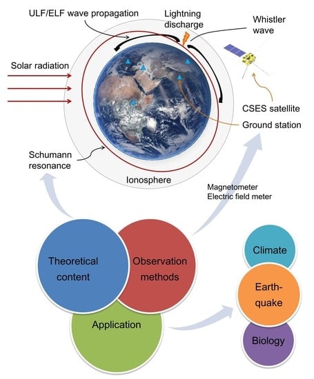
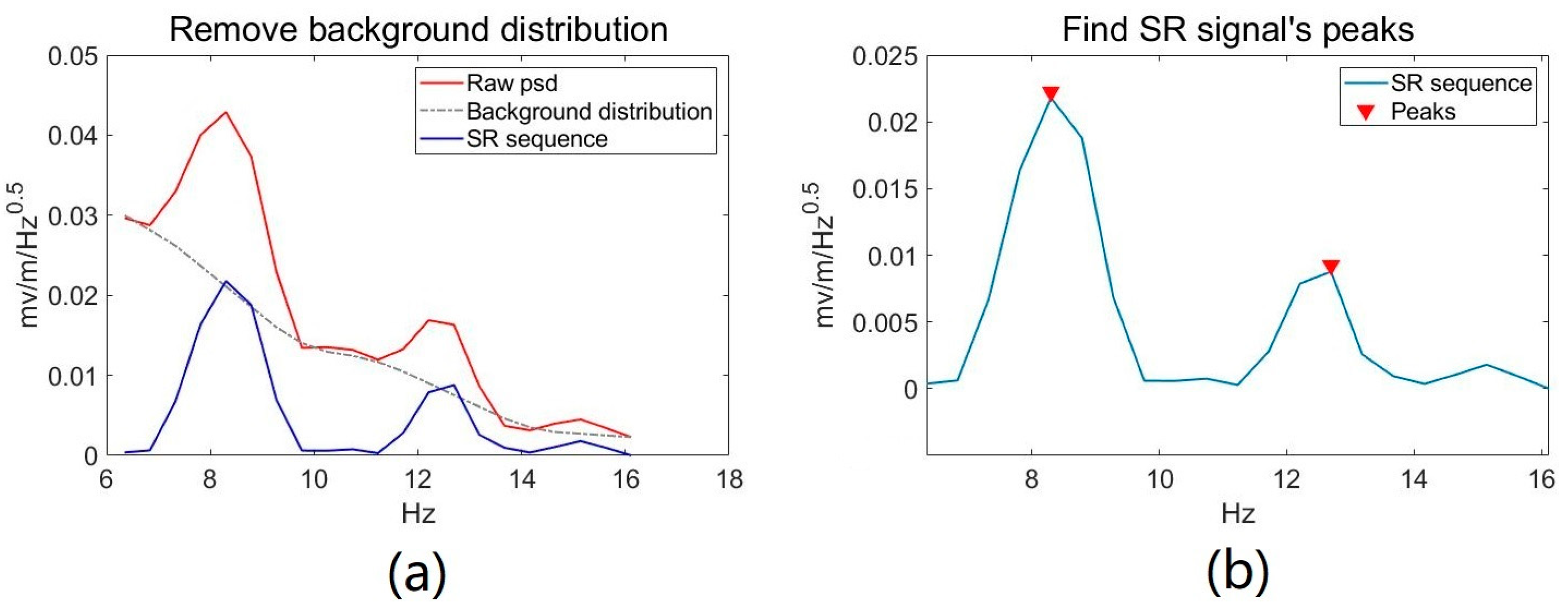
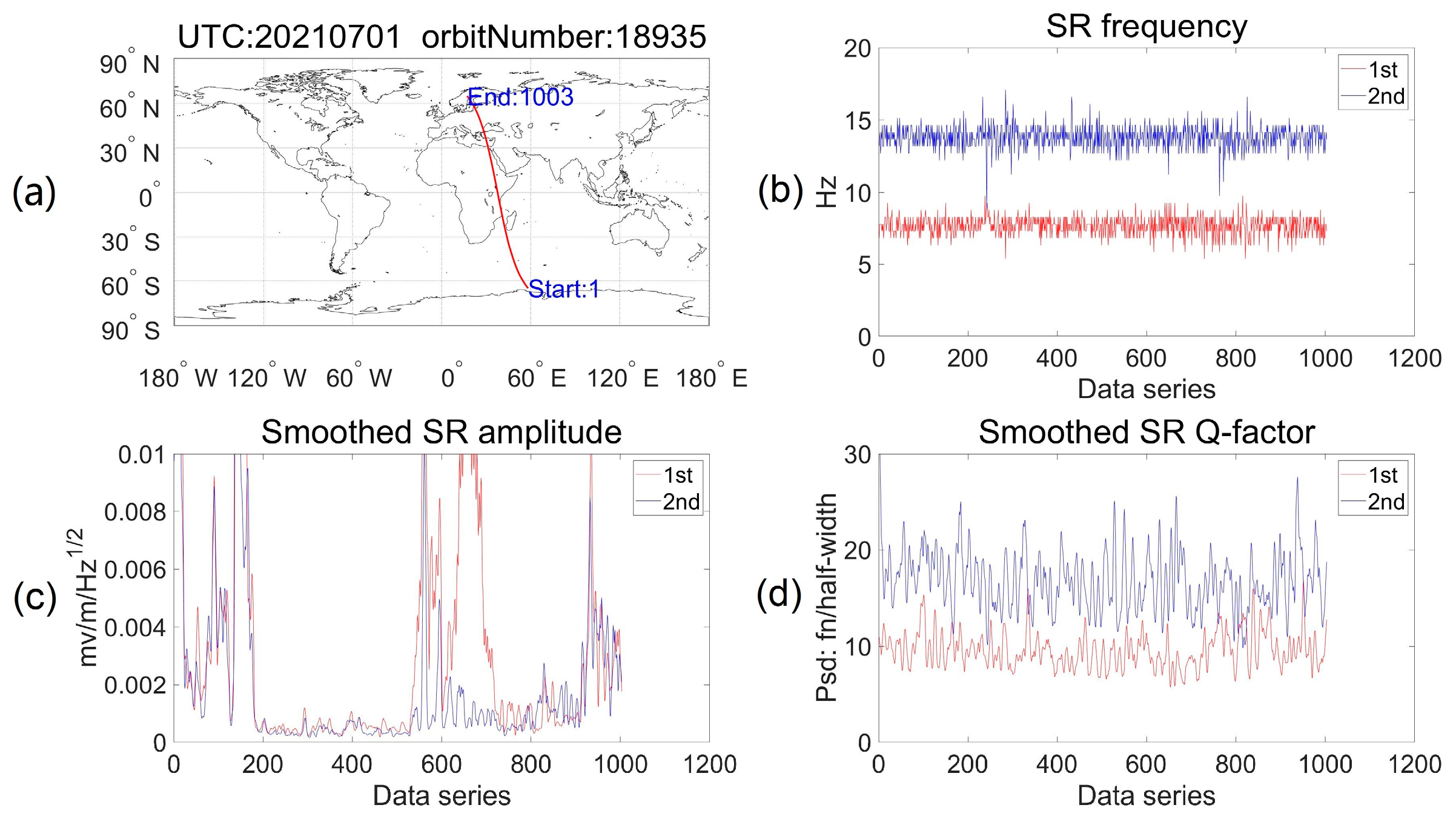
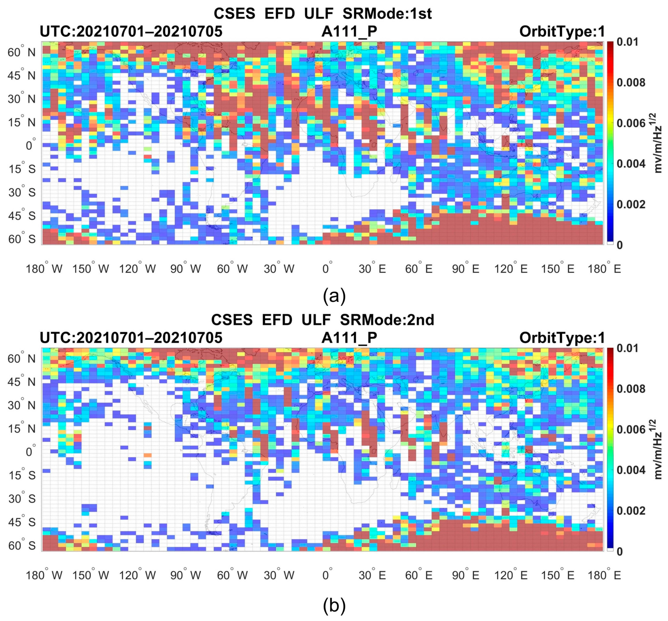
On 2 February 2018, as the first satellite of the Chinese Geophysical Field Satellite Program and the first space-based platform of the China Earthquake Stereoscopic Observation System, the first China Seismo-Electromagnetic Satellite (CSES-01) was launched into orbit [134,135,136]. As shown in Figure 2, Figure 3 and Figure 4, we identified and extracted the signal parameters of the first two modes of SR using the electric field data of the CSES satellite, and plotted the corresponding SR background using all SR parameters in one revisit cycle (5 days).
The methods shown in Figure 2 for removing the background contribution include separating and smoothing the background contribution and removing the smoothed background noise from the original power spectrum. We removed the background contribution of the electric field power spectrum and obtained the parameters of the first two modes of SR signals by identifying the peaks.
As shown in Figure 3, the amplitude trends of SR’s two modes are similar, and the amplitude of SR’s first mode is generally higher than the second mode. When passing through the central African region, the amplitude of SR signals extracted significantly increases (Figure 3a,c). Figure 3d shows that the Q factor also increases as the SR frequency increases. Based on the above methods and results, the SR background field is drawn as shown in Figure 4, which provides a solid foundation for further research on SR signal characteristics and their correlation with events such as earthquakes.
Currently, China’s CSES-02 satellite is in development and will be launched in 2024. With more and more satellites collecting electric field and magnetic field data, SR research based on space-based observations will experience rapid expansion in the future.
Author Contributions
Conceptualization, J.L. and J.H.; methodology, J.L., J.H. and Z.L.; software, J.L., J.H. and Q.W.; validation, J.H., Z.L. and Z.Z. (Zhengyu Zhao); formal analysis, J.H.; investigation, J.L. and J.H.; resources, J.H., Z.Z. (Zhima Zeren) and X.S.; data curation, J.L.; writing—original draft preparation, J.L.; writing—review and editing, J.L., J.H. and Z.Z. (Zhengyu Zhao); visualization, J.L.; supervision, J.H.; project administration, J.H. and Z.Z. (Zhima Zeren); funding acquisition, Z.Z. (Zhima Zeren) and X.S. All authors have read and agreed to the published version of the manuscript.
Funding
This research was jointly funded by the National Natural Science Foundation of China (NSFC) Project, grant number 42104159; the Investigation of the Lithosphere Atmosphere Ionosphere Coupling (LAIC) Mechanism before the Natural Hazards, ISSI 23-583; and the Asia-Pacific Space Cooperation Organization earthquake special project phase 2, ISSI-BJ2019, Dragon 5 Cooperation Proposal, #58892, #59308.
Data Availability Statement
The data of CSES can be downloaded from the website (http://www.leos.ac.cn/). The data used by the article was accessed on 1 February 2023.
Acknowledgments
The authors acknowledge the International Space Science Institute (ISSI in Bern, Switzerland and ISSI-BJ in Beijing, China) for supporting International Team 23-583 lead by Dedalo Marchetti and Essam Ghamry, and wish to thank Ni Binbin and Ouyang Xinyan for their contributions during the SR study based on CSES data.
Conflicts of Interest
The authors declare no conflict of interest.
References
- Nickolaenko, A.P.; Hayakawa, M. Resonances in the Earth-Ionosphere Cavity; Kluwer Academic Publishers: Dordrecht, The Netherlands; Boston, MA, USA; London, UK, 2002. [Google Scholar]
- Sátori, G.; Williams, E.; Mushtak, V. Response of the Earth–Ionosphere Cavity Resonator to the 11-Year Solar Cycle in X-Radiation. J. Atmos. Sol.-Terr. Phys. 2005, 67, 553–562. [Google Scholar] [CrossRef]
- Tran, A.; Polk, C. Schumann Resonances and Electrical Conductivity of the Atmospher and Lower Ionosphere—I. Effects of Conductivity at Various Altitudes on Resonance Frequencies and Attenuation. J. Atmos. Terr. Phys. 1979, 41, 1241–1248. [Google Scholar] [CrossRef]
- Yang, H. Three-Dimensional Finite Difference Time Domain Modeling of the Earth-Ionosphere Cavity Resonances. Geophys. Res. Lett. 2005, 32, L03114. [Google Scholar] [CrossRef] [Green Version]
- Galejs, J. ELF Waves in the Presence of Exponential Ionospheric Conductivity Profiles. IRE Trans. Antennas Propag. 1961, 9, 554–562. [Google Scholar] [CrossRef]
- Bennett, A.J.; Harrison, R.G. Surface Measurement System for the Atmospheric Electrical Vertical Conduction Current Density, with Displacement Current Density Correction. J. Atmos. Sol.-Terr. Phys. 2008, 70, 1373–1381. [Google Scholar] [CrossRef]
- George, F.F.G. Physics at the British Association. Nature 1893, 48, 525–529. [Google Scholar] [CrossRef] [Green Version]
- Larmor, J. Electric Vibrations in Condensing Dielectric Systems. Math. Phys. Pap. 1929, 1, 356–378. [Google Scholar]
- Wilson, C.T.R., III. Investigations on Lighting Discharges and on the Electric Field of Thunderstorms. Philos. Trans. R. Soc. Lond. Ser. Contain. Pap. Math. Phys. Character 1921, 221, 73–115. [Google Scholar] [CrossRef]
- Schelkunoff, S.A. Ultrashort Electromagnetic Waves IV—Guided Propagation. Electr. Eng. 1943, 62, 235–246. [Google Scholar] [CrossRef]
- Rydbeck, O.E. On the Forced Electro-Magnetic Oscillations on Spherical Resonators. Philos. Mag. 1948, 39, 633–644. [Google Scholar] [CrossRef]
- Schumann, W.O. Über Die Strahlungslosen Eigenschwingungen Einer Leitenden Kugel, Die von Einer Luftschicht Und Einer Ionosphärenhülle Umgeben Ist. Z. Für Naturforsch. A 1952, 7, 149–154. [Google Scholar] [CrossRef]
- Schumann, W.O. Über Die Dämpfung Der Elektromagnetischen Eigenschwingungen Des Systems Erde—Luft—Ionosphäre. Z. Für Naturforsch. A 1952, 7, 250–252. [Google Scholar] [CrossRef]
- Schumann, W.O. Über die Ausbreitung sehr langer elektrischer Wellen um die Erde und die Signale des Blitzes. Il Nuovo Cimento 1952, 9, 1116–1138. [Google Scholar] [CrossRef]
- Schumann, W.O. Über die Ausbreitung sehr langer elektrischer Wellen und das Wellenspektrum der Blitzentladung. Naturwissenschaften 1952, 39, 475–476. [Google Scholar] [CrossRef]
- Schumann, W.O. Über Die Ausbreitung Sehr Langer Elektrischer Wellen Und Der Blitzentladung Um Die Erde. Z. Angew. Phys. 1952, 4, 474–480. [Google Scholar]
- Schumann, W.O. Über Die Oberwellenfelder Bei Der Ausbreitung Langer Elektrischer Wellen Um Die Erde Und Die Signale Des Blitzes. Naturwissenschaften 1953, 40, 504–505. [Google Scholar] [CrossRef]
- Schumann, W.O. Über Die Ausbreitung Langer Elektrischer Wellen Um Die Erde Und Einige Anwendungen Auf Senderinterferenzen Und Blitzsignale. Z. Angew. Phys. 1954, 6, 346. [Google Scholar]
- Schumann, W.O. Elektrische Eigenschwingnugen Des Systems Erde-Luft-Ionosphare. Z. Angew. Phys. 1957, 9, 373–378. [Google Scholar]
- Coroniti, S.C.; Hughes, J. Planetary Electrodynamics, the Chapter by Charles Polk; Gordon and Breach Science Publishers Inc: New York, NY, USA, 1969. [Google Scholar]
- Lysak, R.L. Feedback Instability of the Ionospheric Resonant Cavity. J. Geophys. Res. Space Phys. 1991, 96, 1553–1568. [Google Scholar] [CrossRef]
- Balser, M.; Wagner, C.A. Diurnal Power Variations of the Earth-Ionosphere Cavity Modes and Their Relationship to Worldwide Thunderstorm Activity. J. Geophys. Res. 1962, 67, 619–625. [Google Scholar] [CrossRef]
- Egerton, R.F. Electron Energy-Loss Spectroscopy in the TEM. Rep. Prog. Phys. 2009, 72, 016502. [Google Scholar] [CrossRef]
- Madden, T.; Thompson, W. Low-Frequency Electromagnetic Oscillations of the Earth-Ionosphere Cavity. Rev. Geophys. 1965, 3, 211. [Google Scholar] [CrossRef] [Green Version]
- Greifinger, C.; Greifinger, P. Approximate Method for Determining ELF Eigenvalues in the Earth-Ionosphere Waveguide. Radio Sci. 1978, 13, 831–837. [Google Scholar] [CrossRef]
- Mushtak, V.C.; Williams, E.R. ELF Propagation Parameters for Uniform Models of the Earth–Ionosphere Waveguide. J. Atmos. Sol.-Terr. Phys. 2002, 64, 1989–2001. [Google Scholar] [CrossRef]
- Williams, E.R.; Mushtak, V.C.; Nickolaenko, A.P. Distinguishing Ionospheric Models Using Schumann Resonance Spectra. J. Geophys. Res. 2006, 111, D16107. [Google Scholar] [CrossRef] [Green Version]
- Pechony, O.; Price, C.; Nickolaenko, A.P. Relative Importance of the Day-Night Asymmetry in Schumann Resonance Amplitude Records: Relative Importance of Day-Night Asymmetry. Radio Sci. 2007, 42, 1–12. [Google Scholar] [CrossRef] [Green Version]
- Zhou, H.; Yu, H.; Cao, B.; Qiao, X. Diurnal and Seasonal Variations in the Schumann Resonance Parameters Observed at Chinese Observatories. J. Atmos. Sol.-Terr. Phys. 2013, 98, 86–96. [Google Scholar] [CrossRef]
- Ouyang, X.Y.; Zhang, X.M.; Shen, X.H.; Miao, Y.Q. Background features of Schumann resonance observed in Yunnan, southwestern China. J. Geophys. 2013, 56, 1937–1944. (In Chinese) [Google Scholar] [CrossRef]
- Yin, F.; Zhang, Q.L.; Ji, T.T.; Jiang, S. Diurnal variations of Schumann resonances signals in the Earth-ionosphere cavity. J. Meteorol. Sci. 2015, 35, 480–487. (In Chinese) [Google Scholar] [CrossRef]
- Nickolaenko, A.P.; Schekotov, A.Y.; Hayakawa, M.; Romero, R.; Izutsu, J. Electromagnetic Manifestations of Tonga Eruption in Schumann Resonance Band. J. Atmos. Sol.-Terr. Phys. 2022, 237, 105897. [Google Scholar] [CrossRef]
- Bór, J.; Bozóki, T.; Sátori, G.; Williams, E.; Behnke, S.A.; Rycroft, M.J.; Buzás, A.; Silva, H.G.; Kubicki, M.; Said, R.; et al. Responses of the AC/DC Global Electric Circuit to Volcanic Electrical Activity in the Hunga Tonga-Hunga Ha’apai Eruption on 15 January 2022. J. Geophys. Res. Atmos. 2023, 128, e2022JD038238. [Google Scholar] [CrossRef]
- Nickolaenko, A.P.; Shvets, A.V.; Galuk, Y.P.; Schekotov, A.Y.; Hayakawa, M.; Mezentsev, A.; Romero, R.; De Rosa, R.; Kudintseva, I.G. Power Flux in the Schumann Resonance Band Linked to the Eruption of Tonga Volcano on Jan. 15, 2022. (Two Point Measurements of Umov-Poynting Vector). J. Atmos. Sol.-Terr. Phys. 2023, 247, 106078. [Google Scholar] [CrossRef]
- Izvekova, Y.N.; Popel, S.I.; Izvekov, O.Y. Dust and Dusty Plasma Effects in Schumann Resonances on Mars: Comparison with Earth. Icarus 2022, 371, 114717. [Google Scholar] [CrossRef]
- Mezentsev, A.; Nickolaenko, A.P.; Shvets, A.V.; Galuk, Y.P.; Schekotov, A.Y.; Hayakawa, M.; Romero, R.; Izutsu, J.; Kudintseva, I.G. Observational and Model Impact of Tonga Volcano Eruption on Schumann Resonance. J. Geophys. Res. Atmos. 2023, 128, e2022JD037841. [Google Scholar] [CrossRef]
- Gavrilov, B.G.; Poklad, Y.V.; Ryakhovsky, I.A.; Ermak, V.M.; Achkasov, N.S.; Kozakova, E.N. Global Electromagnetic Disturbances Caused by the Eruption of the Tonga Volcano on 15 January 2022. J. Geophys. Res. Atmos. 2022, 127, e2022JD037411. [Google Scholar] [CrossRef]
- Kong, Q.; Li, C.; Shi, K.; Guo, J.; Han, J.; Wang, T.; Bai, Q.; Chen, Y. Global Ionospheric Disturbance Propagation and Vertical Ionospheric Oscillation Triggered by the 2022 Tonga Volcanic Eruption. Atmosphere 2022, 13, 1697. [Google Scholar] [CrossRef]
- Price, C. ELF Electromagnetic Waves from Lightning: The Schumann Resonances. Atmosphere 2016, 7, 116. [Google Scholar] [CrossRef] [Green Version]
- Perotoni, M.B. Eigenmode Prediction of the Schumann Resonances. IEEE Antennas Wirel. Propag. Lett. 2018, 17, 942–945. [Google Scholar] [CrossRef]
- Ni, B.B.; Zhao, Z.Y. Spatial observations of Schumann resonance at the ionospheric altitudes. Chin. J. Geophys. 2005, 48, 744–750. (In Chinese) [Google Scholar] [CrossRef]
- Besser, B.P. Synopsis of the Historical Development of Schumann Resonances: History of Schumann Resonances. Radio Sci. 2007, 42, 1–20. [Google Scholar] [CrossRef]
- Balser, M.; Wagner, C.A. Observations of Earth–Ionosphere Cavity Resonances. Nature 1960, 188, 638–641. [Google Scholar] [CrossRef]
- Ohta, K.; Izutsu, J.; Hayakawa, M. Anomalous Excitation of Schumann Resonances and Additional Anomalous Resonances before the 2004 Mid-Niigata Prefecture Earthquake and the 2007 Noto Hantou Earthquake. Phys. Chem. Earth Parts ABC 2009, 34, 441–448. [Google Scholar] [CrossRef]
- Votis, C.I.; Tatsis, G.; Christofilakis, V.; Chronopoulos, S.K.; Kostarakis, P.; Tritakis, V.; Repapis, C. A New Portable ELF Schumann Resonance Receiver: Design and Detailed Analysis of the Antenna and the Analog Front-End. EURASIP J. Wirel. Commun. Netw. 2018, 2018, 155. [Google Scholar] [CrossRef] [Green Version]
- Cano-Domingo, C.; Castellano, N.N.; Fernandez-Ros, M.; Gazquez-Parra, J.A. Segmentation and Characteristic Extraction for Schumann Resonance Transient Events. Measurement 2022, 194, 110957. [Google Scholar] [CrossRef]
- Tatsis, G.; Christofilakis, V.; Chronopoulos, S.K.; Kostarakis, P.; Nistazakis, H.E.; Repapis, C.; Tritakis, V. Design and Implementation of a Test Fixture for ELF Schumann Resonance Magnetic Antenna Receiver and Magnetic Permeability Measurements. Electronics 2020, 9, 171. [Google Scholar] [CrossRef] [Green Version]
- Coughlin, M.W.; Cirone, A.; Meyers, P.; Atsuta, S.; Boschi, V.; Chincarini, A.; Christensen, N.L.; De Rosa, R.; Effler, A.; Fiori, I.; et al. Measurement and Subtraction of Schumann Resonances at Gravitational-Wave Interferometers. Phys. Rev. D 2018, 97, 102007. [Google Scholar] [CrossRef] [Green Version]
- Silagadze, Z.K. Schumann Resonance Transients and the Search for Gravitational Waves. Mod. Phys. Lett. A 2018, 33, 1850023. [Google Scholar] [CrossRef] [Green Version]
- Fan, Y.; Tang, J.; Zhao, G.Z.; Wang, L.F.; Wu, J.X.; Li, X.S.; Huang, T.B.; Liu, G.K. Schumann resonances variation observed from Electromagnetic monitoring stations. J. Geophys. 2013, 56, 2369–2377. [Google Scholar] [CrossRef]
- Cao, B.X.; Qiao, X.L. Schumann resonance observations in Low ionosphere. J. Electron. Inf. Technol. 2010, 32, 2002–2005. [Google Scholar] [CrossRef]
- Rodríguez-Camacho, J.; Fornieles, J.; Carrión, M.C.; Portí, J.A.; Toledo-Redondo, S.; Salinas, A. On the Need of a Unified Methodology for Processing Schumann Resonance Measurements. J. Geophys. Res. Atmos. 2018, 123, 13277–13290. [Google Scholar] [CrossRef]
- Soler-Ortiz, M.; Ros, M.F.; Castellano, N.N.; Parra, J.A.G. A New Way of Analyzing the Schumann Resonances: A Statistical Approach. IEEE Trans. Instrum. Meas. 2021, 70, 9508811. [Google Scholar] [CrossRef]
- Salinas, A.; Rodríguez-Camacho, J.; Portí, J.; Carrión, M.C.; Fornieles-Callejón, J.; Toledo-Redondo, S. Schumann Resonance Data Processing Programs and Four-Year Measurements from Sierra Nevada ELF Station. Comput. Geosci. 2022, 165, 105148. [Google Scholar] [CrossRef]
- Ogawa, T.; Kozai, K.; Kawamoto, H. Shumann Resonances Observed with a Balloon in the Stratosphere. J. Atmos. Terr. Phys. 1979, 41, 135–142. [Google Scholar] [CrossRef]
- Zhao, Z.Y.; Xie, S.G.; Masson, A.; Lefeuvre, F. Detection of Schumann Resonance in the Ionosphere F Region. Chin. J. Space Sci. 2000, 20, 113–120. [Google Scholar] [CrossRef]
- Simões, F.; Pfaff, R.; Freudenreich, H. Satellite Observations of Schumann Resonances in the Earth’s Ionosphere: Schumann Resonances in the Ionosphere. Geophys. Res. Lett. 2011, 38, L22101. [Google Scholar] [CrossRef]
- Dudkin, D.; Pilipenko, V.; Korepanov, V.; Klimov, S.; Holzworth, R. Electric Field Signatures of the IAR and Schumann Resonance in the Upper Ionosphere Detected by Chibis-M Microsatellite. J. Atmos. Sol.-Terr. Phys. 2014, 117, 81–87. [Google Scholar] [CrossRef]
- Toledo-Redondo, S.; Parrot, M.; Salinas, A. Variation of the First Cut-off Frequency of the Earth-Ionosphere Waveguide Observed by Demeter: Cut-off Frequency Observed by Demeter. J. Geophys. Res. Space Phys. 2012, 117, A04321. [Google Scholar] [CrossRef] [Green Version]
- Nickolaenko, A.P.; Rabinowicz, L.M. Study of the Annual Changes of Global Lightning Distribution and Frequency Variations of the First Schumann Resonance Mode. J. Atmos. Terr. Phys. 1995, 57, 1345–1348. [Google Scholar] [CrossRef]
- Tatsis, G.; Sakkas, A.; Christofilakis, V.; Baldoumas, G.; Chronopoulos, S.K.; Paschalidou, A.K.; Kassomenos, P.; Petrou, I.; Kostarakis, P.; Repapis, C.; et al. Correlation of Local Lightning Activity with Extra Low Frequency Detector for Schumann Resonance Measurements. Sci. Total Environ. 2021, 787, 147671. [Google Scholar] [CrossRef]
- Koloskov, A.V.; Nickolaenko, A.P.; Yampolsky, Y.M.; Hall, C.; Budanov, O.V. Variations of Global Thunderstorm Activity Derived from the Long-Term Schumann Resonance Monitoring in the Antarctic and in the Arctic. J. Atmos. Sol.-Terr. Phys. 2020, 201, 105231. [Google Scholar] [CrossRef]
- Price, C.; Melnikov, A. Diurnal, Seasonal and Inter-Annual Variations in the Schumann Resonance Parameters. J. Atmos. Sol.-Terr. Phys. 2004, 66, 1179–1185. [Google Scholar] [CrossRef]
- Ghosh, A.; Biswas, D.; Hazra, P.; Guha, G.; De, S.S. Studies on Schumann Resonance Phenomena and Some Recent Advancements. Geomagn. Aeron. 2019, 59, 980–994. [Google Scholar] [CrossRef]
- Shvets, A.V.; Hobara, Y.; Hayakawa, M. Variations of the Global Lightning Distribution Revealed from Three-Station Schumann Resonance Measurements: Global Lightning Distributions at ELF. J. Geophys. Res. Space Phys. 2010, 115, A12316. [Google Scholar] [CrossRef] [Green Version]
- Yamashita, K.; Takahashi, Y.; Sato, M.; Kase, H. Improvement in Lightning Geolocation by Time-of-Arrival Method Using Global ELF Network Data: Time-of-Arrival Method. J. Geophys. Res. Space Phys. 2011, 116, A00E61. [Google Scholar] [CrossRef]
- Prácser, E.; Bozóki, T.; Sátori, G.; Williams, E.; Guha, A.; Yu, H. Reconstruction of Global Lightning Activity Based on Schumann Resonance Measurements: Model Description and Synthetic Tests. Radio Sci. 2019, 54, 254–267. [Google Scholar] [CrossRef]
- Boldi, R.; Williams, E.; Guha, A. Determination of the Global-Average Charge Moment of a Lightning Flash Using Schumann Resonances and the LIS/OTD Lightning Data. J. Geophys. Res. Atmos. 2018, 123, 108–123. [Google Scholar] [CrossRef] [Green Version]
- Williams, E.; Mareev, E. Recent Progress on the Global Electrical Circuit. Atmos. Res. 2014, 135–136, 208–227. [Google Scholar] [CrossRef]
- Zhu, R.P.; Yuan, T.; Li, W.L.; Na, G.W. Characteristics of global lightning activities based on satellite observations. Clim. Environ. Res. 2013, 18, 639–650. (In Chinese) [Google Scholar] [CrossRef]
- Cecil, D.J.; Buechler, D.E.; Blakeslee, R.J. Gridded Lightning Climatology from TRMM-LIS and OTD: Dataset Description. Atmos. Res. 2014, 135–136, 404–414. [Google Scholar] [CrossRef] [Green Version]
- Ni, X.; Hui, W.; Zhang, Q.; Huang, F.; Liu, C. Comparison of Lightning Detection Between the FY-4A Lightning Mapping Imager and the ISS Lightning Imaging Sensor. Earth Space Sci. 2021, 8, e2020EA001099. [Google Scholar] [CrossRef]
- Rodger, C.J.; Werner, S.; Brundell, J.B.; Lay, E.H.; Thomson, N.R.; Holzworth, R.H.; Dowden, R.L. Detection Efficiency of the VLF World-Wide Lightning Location Network (WWLLN): Initial Case Study. Ann. Geophys. 2006, 24, 3197–3214. [Google Scholar] [CrossRef] [Green Version]
- Huang, E.; Williams, E.; Boldi, R.; Heckman, S.; Lyons, W.; Taylor, M.; Nelson, T.; Wong, C. Criteria for Sprites and Elves Based on Schumann Resonance Observations. J. Geophys. Res. Atmos. 1999, 104, 16943–16964. [Google Scholar] [CrossRef]
- Hayakawa, M.; Hobara, Y.; Suzuki, T. Lightning Effects in the Mesosphere and Ionosphere. Light. Electromagn. 2012, 16, 611–646. [Google Scholar] [CrossRef]
- Chern, J.L.; Hsu, R.R.; Su, H.T.; Mende, S.B.; Fukunishi, H.; Takahashi, Y.; Lee, L.C. Global Survey of Upper Atmospheric Transient Luminous Events on the ROCSAT-2 Satellite. J. Atmos. Sol.-Terr. Phys. 2003, 65, 647–659. [Google Scholar] [CrossRef]
- Neubert, T.; Allin, T.H.; Blanc, E.; Farges, T.; Haldoupis, C.; Mika, A.; Soula, S.; Knutsson, L.; van der Velde, O.; Marshall, R.A.; et al. Co-Ordinated Observations of Transient Luminous Events during the EuroSprite2003 Campaign. J. Atmos. Sol.-Terr. Phys. 2005, 67, 807–820. [Google Scholar] [CrossRef]
- Yair, Y.; Price, C.; Levin, Z.; Joseph, J.; Israelevitch, P.; Devir, A.; Moalem, M.; Ziv, B.; Asfur, M. Sprite Observations from the Space Shuttle during the Mediterranean Israeli Dust Experiment (MEIDEX). J. Atmos. Sol.-Terr. Phys. 2003, 65, 635–642. [Google Scholar] [CrossRef]
- Yair, Y.; Price, C.; Ganot, M.; Greenberg, E.; Yaniv, R.; Ziv, B.; Sherez, Y.; Devir, A.; Bór, J.; Sátori, G. Optical Observations of Transient Luminous Events Associated with Winter Thunderstorms near the Coast of Israel. Atmos. Res. 2009, 91, 529–537. [Google Scholar] [CrossRef]
- Nickolaenko, A.P.; Hayakawa, M.; Hobara, Y. Q-Bursts: Natural ELF Radio Transients. Surv. Geophys. 2010, 31, 409–425. [Google Scholar] [CrossRef]
- Ogawa, T.; Komatsu, M. Q-Bursts from Various Distances on the Earth. Atmos. Res. 2009, 91, 538–545. [Google Scholar] [CrossRef]
- Ogawa, T.; Komatsu, M. Propagation Velocity of VLF EM Waves from Lightning Discharges Producing Q-Bursts Observed in the Range 10–15Mm. Atmos. Res. 2010, 95, 101–107. [Google Scholar] [CrossRef]
- Bór, J.; Ludván, B.; Attila, N.; Steinbach, P. Systematic Deviations in Source Direction Estimates of Q-Bursts Recorded at Nagycenk, Hungary: On Deviations of ELF Source Directions. J. Geophys. Res. Atmos. 2016, 121, 5601–5619. [Google Scholar] [CrossRef] [Green Version]
- Yair, Y.; Fischer, G.; Simões, F.; Renno, N.; Zarka, P. Updated Review of Planetary Atmospheric Electricity. Space Sci. Rev. 2008, 137, 29–49. [Google Scholar] [CrossRef]
- Pechony, O.; Price, C. Schumann Resonance Parameters Calculated with a Partially Uniform Knee Model on Earth, Venus, Mars, and Titan: Schumann Resonance Model. Radio Sci. 2004, 39, 1–10. [Google Scholar] [CrossRef]
- Yang, H.; Pasko, V.P.; Yair, Y. Three-Dimensional Finite Difference Time Domain Modeling of the Schumann Resonance Parameters on Titan, Venus, and Mars: Schumann Resonances on Titan, Venus, and Mars. Radio Sci. 2006, 41, 1–10. [Google Scholar] [CrossRef]
- Béghin, C.; Canu, P.; Karkoschka, E.; Sotin, C.; Bertucci, C.; Kurth, W.S.; Berthelier, J.J.; Grard, R.; Hamelin, M.; Schwingenschuh, K.; et al. New Insights on Titan’s Plasma-Driven Schumann Resonance Inferred from Huygens and Cassini Data. Planet. Space Sci. 2009, 57, 1872–1888. [Google Scholar] [CrossRef]
- Béghin, C.; Randriamboarison, O.; Hamelin, M.; Karkoschka, E.; Sotin, C.; Whitten, R.C.; Berthelier, J.-J.; Grard, R.; Simões, F. Analytic Theory of Titan’s Schumann Resonance: Constraints on Ionospheric Conductivity and Buried Water Ocean. Icarus 2012, 218, 1028–1042. [Google Scholar] [CrossRef] [Green Version]
- Cano Domingo, C.; Fernandez Ros, M.; Novas Castellano, N.; Parra, J.A.G. Diurnal and Seasonal Results of the Schumann Resonance Observatory in Sierra De Filabres, Spain. IEEE Trans. Antennas Propag. 2021, 69, 6680–6690. [Google Scholar] [CrossRef]
- Domingo, C.C.; Castellano, N.N.; Stoean, R.; Fernandez-Ros, M.; Gazquez Parra, J.A. Schumann Resonance Modes and Ionosphere Parameters: An Annual Variability Comparison. IEEE Trans. Instrum. Meas. 2022, 71, 6005410. [Google Scholar] [CrossRef]
- Cano-Domingo, C.; Stoean, R.; Joya, G.; Novas, N.; Fernandez-Ros, M.; Gazquez, J.A. A Machine Learning Hourly Analysis on the Relation the Ionosphere and Schumann Resonance Frequency. Measurement 2023, 208, 112426. [Google Scholar] [CrossRef]
- Kulak, A. Solar Variations in Extremely Low Frequency Propagation Parameters: 1. A Two-Dimensional Telegraph Equation (TDTE) Model of ELF Propagation and Fundamental Parameters of Schumann Resonances. J. Geophys. Res. 2003, 108, 1270. [Google Scholar] [CrossRef]
- Kulak, A. Solar Variations in Extremely Low Frequency Propagation Parameters: 2. Observations of Schumann Resonances and Computation of the ELF Attenuation Parameter. J. Geophys. Res. 2003, 108, 1271. [Google Scholar] [CrossRef]
- Sátori, G.; Williams, E.; Price, C.; Boldi, R.; Koloskov, A.; Yampolski, Y.; Guha, A.; Barta, V. Effects of Energetic Solar Emissions on the Earth–Ionosphere Cavity of Schumann Resonances. Surv. Geophys. 2016, 37, 757–789. [Google Scholar] [CrossRef] [Green Version]
- Bozóki, T.; Sátori, G.; Williams, E.; Mironova, I.; Steinbach, P.; Bland, E.C.; Koloskov, A.; Yampolski, Y.M.; Budanov, O.V.; Neska, M.; et al. Solar Cycle-Modulated Deformation of the Earth–Ionosphere Cavity. Front. Earth Sci. 2021, 9, 689127. [Google Scholar] [CrossRef]
- Kudintseva, I.G.; Galuk, Y.P.; Nickolaenko, A.P.; Hayakawa, M. Modifications of Middle Atmosphere Conductivity during Sudden Ionospheric Disturbances Deduced from Changes of Schumann Resonance Peak Frequencies. Radio Sci. 2018, 53, 670–682. [Google Scholar] [CrossRef]
- Beggan, C.D.; Musur, M. Observation of Ionospheric Alfvén Resonances at 1–30 Hz and Their Superposition with the Schumann Resonances. J. Geophys. Res. Space Phys. 2018, 123, 4202–4214. [Google Scholar] [CrossRef] [Green Version]
- Pazos, M.; Mendoza, B.; Sierra, P.; Andrade, E.; Rodríguez, D.; Mendoza, V.; Garduño, R. Analysis of the Effects of Geomagnetic Storms in the Schumann Resonance Station Data in Mexico. J. Atmos. Sol.-Terr. Phys. 2019, 193, 105091. [Google Scholar] [CrossRef]
- Hayakawa, M.; Hobara, Y.; Ohta, K.; Izutsu, J.; Nickolaenko, A.P.; Sorokin, V. Seismogenic Effects in the ELF Schumann Resonance Band. IEEJ Trans. Fundam. Mater. 2011, 131, 684–690. [Google Scholar] [CrossRef]
- Schekotov, A.Y.; Molchanov, O.A.; Hayakawa, M.; Fedorov, E.N.; Chebrov, V.N.; Sinitsin, V.I.; Gordeev, E.E.; Belyaev, G.G.; Yagova, N.V. ULF/ELF Magnetic Field Variations from Atmosphere Induced by Seismicity: ULF/ELF Electromagnetic Emission. Radio Sci. 2007, 42, 1–13. [Google Scholar] [CrossRef]
- Molchanov, O.A.; Hayakawa, M. Seismo-Electromagnetics and Related Phenomena: History and Latest Results; Terrapub: Tokyo, Japan, 2008. [Google Scholar]
- Ohta, K.; Watanabe, N.; Hayakawa, M. Survey of Anomalous Schumann Resonance Phenomena Observed in Japan, in Possible Association with Earthquakes in Taiwan. Phys. Chem. Earth Parts ABC 2006, 31, 397–402. [Google Scholar] [CrossRef]
- De, S.S.; De, B.K.; Bandyopadhyay, B.; Paul, S.; Haldar, D.K.; Barui, S. Studies on the Shift in the Frequency of the First Schumann Resonance Mode during a Solar Proton Event. J. Atmos. Sol.-Terr. Phys. 2010, 72, 829–836. [Google Scholar] [CrossRef]
- Hayakawa, M.; Ohta, K.; Nickolaenko, A.P.; Ando, Y. Anomalous Effect in Schumann Resonance Phenomena Observed in Japan, Possibly Associated with the Chi-Chi Earthquake in Taiwan. Ann. Geophys. 2005, 23, 1335–1346. [Google Scholar] [CrossRef] [Green Version]
- Hayakawa, M.; Nickolaenko, A.P.; Sekiguchi, M.; Yamashita, K.; Ida, Y.; Yano, M. Anomalous ELF Phenomena in the Schumann Resonance Band as Observed at Moshiri (Japan) in Possible Association with an Earthquake in Taiwan. Nat. Hazards Earth Syst. Sci. 2008, 8, 1309–1316. [Google Scholar] [CrossRef]
- Nickolaenko, A.P.; Galuk, Y.P.; Hayakawa, M. The Effect of a Compact Ionosphere Disturbance over the Earthquake: A Focus on Schumann Resonance. Int. J. Electron. Appl. Res. 2018, 5, 11–39. [Google Scholar] [CrossRef]
- Christofilakis, V.; Tatsis, G.; Votis, C.; Contopoulos, I.; Repapis, C.; Tritakis, V. Significant ELF Perturbations in the Schumann Resonance Band before and during a Shallow Mid-Magnitude Seismic Activity in the Greek Area (Kalpaki). J. Atmos. Sol.-Terr. Phys. 2019, 182, 138–146. [Google Scholar] [CrossRef]
- Galuk, Y.P.; Kudintseva, I.G.; Nickolaenko, A.P.; Hayakawa, M. Modifications of Schumann Resonance Spectra as an Estimate of Causative Earthquake Magnitude: The Model Treatment. J. Atmos. Sol.-Terr. Phys. 2020, 209, 105392. [Google Scholar] [CrossRef]
- Sierra Figueredo, P.; Mendoza Ortega, B.; Pazos, M.; Rodríguez Osorio, D.; Andrade Mascote, E.; Mendoza, V.M.; Garduño, R. Schumann Resonance Anomalies Possibly Associated with Large Earthquakes in Mexico. Indian J. Phys. 2021, 95, 1959–1966. [Google Scholar] [CrossRef]
- Tritakis, V.; Contopoulos, I.; Mlynarczyk, J.; Christofilakis, V.; Tatsis, G.; Repapis, C. How Effective and Prerequisite Are Electromagnetic Extremely Low Frequency (ELF) Recordings in the Schumann Resonances Band to Function as Seismic Activity Precursors. Atmosphere 2022, 13, 185. [Google Scholar] [CrossRef]
- Hayakawa, M.; Izutsu, J.; Schekotov, A.Y.; Nickolaenko, A.P.; Galuk, Y.P.; Kudintseva, I.G. Anomalies of Schumann Resonances as Observed near Nagoya Associated with Two Huge (M~7) Tohoku Offshore Earthquakes in 2021. J. Atmos. Sol.-Terr. Phys. 2021, 225, 105761. [Google Scholar] [CrossRef]
- Zhou, H.; Zhou, Z.; Qiao, X.; Yu, H. Anomalous Phenomena in Schumann Resonance Band Observed in China before the 2011 Magnitude 9.0 Tohoku-Oki Earthquake in Japan: SR Anomalies before a Large Earthquake. J. Geophys. Res. Atmos. 2013, 118, 13338–13345. [Google Scholar] [CrossRef]
- Williams, E.R. The Schumann Resonance: A Global Tropical Thermometer. Science 1992, 256, 1184–1187. [Google Scholar] [CrossRef]
- Price, C.; Asfur, M. Can Lightning Observations Be Used as an Indicator of Upper-Tropospheric Water Vapor Variability? Bull. Am. Meteorol. Soc. 2006, 87, 291–298. [Google Scholar] [CrossRef]
- Sátori, G.; Williams, E.; Lemperger, I. Variability of Global Lightning Activity on the ENSO Time Scale. Atmos. Res. 2009, 91, 500–507. [Google Scholar] [CrossRef]
- Sátori, G.; Zieger, B. El Niňo Related Meridional Oscillation of Global Lightning Activity. Geophys. Res. Lett. 1999, 26, 1365–1368. [Google Scholar] [CrossRef]
- Wang, C.; Deser, C.; Yu, J.-Y.; DiNezio, P.; Clement, A. El Niño and Southern Oscillation (ENSO): A Review. In Coral Reefs of the Eastern Tropical Pacific; Glynn, P.W., Manzello, D.P., Enochs, I.C., Eds.; Coral Reefs of the World; Springer: Dordrecht, The Netherlands, 2017; Volume 8, pp. 85–106. ISBN 978-94-017-7498-7. [Google Scholar]
- Bozóki, T.; Williams, E.; Satori, G.; Beggan, C.D.; Price, C.; Steinbach, P.; Guha, A.; Liu, Y.; Neska, A.; Boldi, R.; et al. Predicting the Occurrence of Extreme El Nino Events Based on Schumann Resonancemeasurements? In Proceedings of the 24th EGU General Assembly, Vienna, Austria, 23–27 May 2022. [Google Scholar]
- Williams, E.; Bozóki, T.; Sátori, G.; Price, C.; Steinbach, P.; Guha, A.; Liu, Y.; Beggan, C.D.; Neska, M.; Boldi, R.; et al. Evolution of Global Lightning in the Transition from Cold to Warm Phase Preceding Two Super El Niño Events. J. Geophys. Res. Atmos. 2021, 126, e2020JD033526. [Google Scholar] [CrossRef]
- Beggan, C.D.; Musur, M.A. Is the Madden–Julian Oscillation Reliably Detectable in Schumann Resonances? J. Atmos. Sol.-Terr. Phys. 2019, 190, 108–116. [Google Scholar] [CrossRef] [Green Version]
- Kozlov, A.V.; Slyunyaev, N.N.; Ilin, N.V.; Sarafanov, F.G.; Frank-Kamenetsky, A.V. The Effect of the Madden–Julian Oscillation on the Global Electric Circuit. Atmos. Res. 2023, 284, 106585. [Google Scholar] [CrossRef]
- Balser, M.; Wagner, C.A. Effect of a High-Altitude Nuclear Detonation on the Earth-Ionosphere Cavity. J. Geophys. Res. 1963, 68, 4115–4118. [Google Scholar] [CrossRef]
- Wait, J. Historical Background and Introduction to the Special Issue on Extremely Low Frequency (ELF) Communications. IEEE Trans. Commun. 1974, 22, 353–354. [Google Scholar] [CrossRef]
- Wait, J. Propagation of ELF Electromagnetic Waves and Project Sanguine/Seafarer. IEEE J. Ocean. Eng. 1977, 2, 161–172. [Google Scholar] [CrossRef]
- Cherry, N.J. Human Intelligence: The Brain, an Electromagnetic System Synchronised by the Schumann Resonance Signal. Med. Hypotheses 2003, 60, 843–844. [Google Scholar] [CrossRef] [Green Version]
- Cherry, N. Schumann Resonances, a Plausible Biophysical Mechanism for the Human Health Effects of Solar. Nat. Hazards 2002, 26, 279–331. [Google Scholar] [CrossRef]
- Danho, S.; Schoellhorn, W.; Aclan, M. Innovative Technical Implementation of the Schumann Resonances and Its Influence on Organisms and Biological Cells. IOP Conf. Ser. Mater. Sci. Eng. 2019, 564, 012081. [Google Scholar] [CrossRef]
- Elhalel, G.; Price, C.; Fixler, D.; Shainberg, A. Cardioprotection from Stress Conditions by Weak Magnetic Fields in the Schumann Resonance Band. Sci. Rep. 2019, 9, 1645. [Google Scholar] [CrossRef] [PubMed] [Green Version]
- Fdez-Arroyabe, P.; Fornieles-Callejón, J.; Santurtún, A.; Szangolies, L.; Donner, R.V. Schumann Resonance and Cardiovascular Hospital Admission in the Area of Granada, Spain: An Event Coincidence Analysis Approach. Sci. Total Environ. 2020, 705, 135813. [Google Scholar] [CrossRef] [PubMed]
- Fdez-Arroyabe, P.; Kourtidis, K.; Haldoupis, C.; Savoska, S.; Matthews, J.; Mir, L.M.; Kassomenos, P.; Cifra, M.; Barbosa, S.; Chen, X.; et al. Glossary on Atmospheric Electricity and Its Effects on Biology. Int. J. Biometeorol. 2021, 65, 5–29. [Google Scholar] [CrossRef]
- Hunting, E.R.; Matthews, J.; De Arróyabe Hernáez, P.F.; England, S.J.; Kourtidis, K.; Koh, K.; Nicoll, K.; Harrison, R.G.; Manser, K.; Price, C.; et al. Challenges in Coupling Atmospheric Electricity with Biological Systems. Int. J. Biometeorol. 2021, 65, 45–58. [Google Scholar] [CrossRef]
- Price, C.; Williams, E.; Elhalel, G.; Sentman, D. Natural ELF Fields in the Atmosphere and in Living Organisms. Int. J. Biometeorol. 2021, 65, 85–92. [Google Scholar] [CrossRef]
- Sukhov, V.; Sukhova, E.; Sinitsyna, Y.; Gromova, E.; Mshenskaya, N.; Ryabkova, A.; Ilin, N.; Vodeneev, V.; Mareev, E.; Price, C. Influence of Magnetic Field with Schumann Resonance Frequencies on Photosynthetic Light Reactions in Wheat and Pea. Cells 2021, 10, 149. [Google Scholar] [CrossRef]
- Huang, J.; Shen, X.; Zhang, X.; Lu, H.; Tan, Q.; Wang, Q.; Yan, R.; Chu, W.; Yang, Y.; Liu, D.; et al. Application System and Data Description of the China Seismo-Electromagnetic Satellite. Earth Planet. Phys. 2018, 2, 444–454. [Google Scholar] [CrossRef]
- Wang, L.W.; Hu, Z.; Shen, X.H.; Zhang, X.G.; Huang, J.P.; Zhang, Y.; Yang, Y.Y. Data processing methods and procedures of CSES satellite. J. Remote Sens. 2018, 22 (Suppl. S1), 39–55. (In Chinese) [Google Scholar] [CrossRef]
- Shen, X.H.; Zhang, X.M.; Cui, J.; Zhou, X.; Jiang, W.L.; Gong, L.X.; Li, Y.S.; Liu, Q.Q. Remote sensing application in earthquake science research and geophysical fields exploration satellite mission in China. J. Remote Sens. 2018, 22 (Suppl. S1), 1–16. (In Chinese) [Google Scholar] [CrossRef]
Figure 1.
The first publicly composite published spectrum of Schumann Resonances. The figure is readapted with permission from Ref. [43]. 1960, M. Balser et al.
Figure 1.
The first publicly composite published spectrum of Schumann Resonances. The figure is readapted with permission from Ref. [43]. 1960, M. Balser et al.

Figure 2.
The extraction method of SR parameters: (a) represents the process of removing the background contribution of the original power spectrum of the electric field, and (b) shows the method of locating and extracting the SR parameters.
Figure 2.
The extraction method of SR parameters: (a) represents the process of removing the background contribution of the original power spectrum of the electric field, and (b) shows the method of locating and extracting the SR parameters.

Figure 3.
SR variation along the orbit at night: (a) shows the geographical position of the satellite orbit, (b–d) correspond to the SR frequency, amplitude, and quality factor extracted from this orbit, respectively. The red line represents SR’s first mode and the blue line represents SR’s second mode.

Figure 4.
Global SR amplitude background: (a,b) represent the global background distribution of the amplitude of the first and second modes of SR, respectively.
Figure 4.
Global SR amplitude background: (a,b) represent the global background distribution of the amplitude of the first and second modes of SR, respectively.

Disclaimer/Publisher’s Note: The statements, opinions and data contained in all publications are solely those of the individual author(s) and contributor(s) and not of MDPI and/or the editor(s). MDPI and/or the editor(s) disclaim responsibility for any injury to people or property resulting from any ideas, methods, instructions or products referred to in the content. |
© 2023 by the authors. Licensee MDPI, Basel, Switzerland. This article is an open access article distributed under the terms and conditions of the Creative Commons Attribution (CC BY) license (https://creativecommons.org/licenses/by/4.0/).
Share and Cite
MDPI and ACS Style
Liu, J.; Huang, J.; Li, Z.; Zhao, Z.; Zeren, Z.; Shen, X.; Wang, Q. Recent Advances and Challenges in Schumann Resonance Observations and Research. Remote Sens. 2023, 15, 3557. https://doi.org/10.3390/rs15143557
AMA Style
Liu J, Huang J, Li Z, Zhao Z, Zeren Z, Shen X, Wang Q. Recent Advances and Challenges in Schumann Resonance Observations and Research. Remote Sensing. 2023; 15(14):3557. https://doi.org/10.3390/rs15143557
Chicago/Turabian StyleLiu, Jinlai, Jianping Huang, Zhong Li, Zhengyu Zhao, Zhima Zeren, Xuhui Shen, and Qiao Wang. 2023. "Recent Advances and Challenges in Schumann Resonance Observations and Research" Remote Sensing 15, no. 14: 3557. https://doi.org/10.3390/rs15143557
Note that from the first issue of 2016, this journal uses article numbers instead of page numbers. See further details here.