

A Graph Memory Neural Network for Sea Surface Temperature Prediction
by
 , ,
, ,
Shuchen Liang
1,2,
Anming Zhao
1,2,
Mengjiao Qin
1,2,
Linshu Hu
1,2,*,
Sensen Wu
1,2,
Zhenhong Du
1,2 and
Renyi Liu
1,2 1
School of Earth Sciences, Zhejiang University, 866 Yuhangtang Rd, Hangzhou 310058, China
2
Zhejiang Provincial Key Laboratory of Geographic Information Scaience, 866 Yuhangtang Rd, Hangzhou 310058, China
*
Author to whom correspondence should be addressed.
Remote Sens. 2023, 15(14), 3539; https://doi.org/10.3390/rs15143539
Submission received: 12 May 2023
/
Revised: 2 July 2023
/
Accepted: 11 July 2023
/
Published: 14 July 2023
(This article belongs to the Special Issue AI for Marine, Ocean and Climate Change Monitoring)
Abstract
:Sea surface temperature (SST) is a key factor in the marine environment, and its accurate forecasting is important for climatic research, ecological preservation, and economic progression. Existing methods mostly rely on convolutional networks, which encounter difficulties in encoding irregular data. In this paper, allowing for comprehensive encoding of irregular data containing land and islands, we construct a graph structure to represent SST data and propose a graph memory neural network (GMNN). The GMNN includes a graph encoder built upon the iterative graph neural network (GNN) idea to extract spatial relationships within SST data. It not only considers node but also edge information, thereby adequately characterizing spatial correlations. Then, a long short-term memory (LSTM) network is used to capture temporal dynamics in the SST variation process. We choose the data from the Northwest Pacific Ocean to validate GMNN’s effectiveness for SST prediction in different partitions, time scales, and prediction steps. The results show that our model has better performance for both complete and incomplete sea areas compared to other models.
1. Introduction
Sea surface temperature (SST) is a crucial variable in marine environments [1]. Changes in SST can greatly impact the climate. Persistent anomalies in SST, characterized by unusually warm or cold conditions, may give rise to phenomena such as El Niño and La Niña [2,3]. Additionally, SST serves to guide marine activities by analyzing its influence on fish migration, which in turn informs fishery distribution and policy formulation [4,5]. It also plays an important role in forecasting marine disasters such as storm surges and red tides [6,7]. Thus, it is evident that accurate prediction of SST has great significance for the marine economy, ecology, and disaster forecasting.
Existing SST prediction methods can be divided into two major categories: numerical methods and data-driven methods. Numerical methods are based on a series of physicochemical parameters, constructing complex equations according to the principles of dynamics and thermodynamics [8,9,10]. However, they demand substantial computational resources and accurate parameter selection for precise results. Data-driven methods, on the other hand, learn patterns directly from the data [11] and have evolved from traditional statistical approaches to machine learning and deep learning techniques. Markov, canonical correlation analysis (CCA), and other statistical approaches are widely used to predict SST [12,13,14], but these models may lack accuracy when dealing with complex nonlinear problems due to their weak nonlinear fitting ability [15]. Therefore, machine learning approaches capable of addressing nonlinear problems are garnering attention in SST prediction research. For example, researchers use support vector machine (SVM) and artificial neural networks (ANN) and achieve promising results [16,17,18].
Machine learning methods require manual feature engineering which can be time-consuming, with their accuracy dependent on the quality of features. Furthermore, deep learning methods automatically extract useful features from big data and can achieve higher accuracy than traditional machine learning methods. As a result, deep learning techniques are becoming increasingly popular for SST prediction. Recurrent neural networks (RNN), including long short-term memory (LSTM) and gated recurrent unit (GRU) variants, excel in processing sequences, making them suitable for time series prediction tasks. Zhang et al. [19] pioneered the use of deep learning in SST prediction by developing an FC-LSTM model, which combined an LSTM layer with a fully connected layer. This approach outperformed support vector regression (SVR) and multilayer perceptron (MLP) in terms of prediction accuracy.
In fact, SST is a variable with spatiotemporal properties, showing dynamic and nonlinear characteristics. However, previous works overlook the spatial features of SST, which limits the prediction accuracy of SST [20]. To fully consider spatial information, researchers generally adopt two approaches. The first one is to use spatial data, such as latitude, longitude, and regional features, as input for the model [21,22]. The second approach is to employ convolutional neural networks (CNN) to extract spatial features at different scales, and integrates them with time series prediction models to form a comprehensive spatiotemporal forecasting method [23,24,25].
Among methods based on convolutional idea, ConvLSTM and its variant, ConvGRU, proposed by Shi et al. [26] in 2015 for precipitation forecasting are widely applied in SST prediction tasks [21,27,28,29], owing to their effectiveness in capturing spatiotemporal correlations. These methods treat SST data as regular images, but in actual research, areas containing land or islands may lack valid data. Standard matrix convolution kernels cannot directly extract information from these locations, and filling in missing values may impact the prediction accuracy at the land-sea boundaries [30].
In recent years, graph neural networks (GNN) have succeeded in areas such as traffic flow prediction, weather forecasting, and disease risk assessment [31]. Graph structures are well-suited for irregular data, and GNNs’ message-passing mechanisms [32] capture adjacency relationships better than CNN, effectively extracting data features. Therefore, in SST prediction, researchers start to explore how to learn SST’s spatial relationships based on graph structures [30,33,34,35]. Among them, most methods use graph convolutional networks (GCN) to update and aggregate the representations of nodes along with their neighboring nodes.
In this study, we propose a graph memory neural network (GMNN) for SST prediction based on GNN idea. First, we develop an SST graph representation using distance threshold and Pearson correlation coefficient to fully express spatial information in irregular regions. An innovation of our model lies in adequately expressing spatial information for these incomplete areas using graph representations. Next, we design a graph encoder using iterative GNN to encode spatial relationships that take into account not only node but also edge features.
Finally, a GMNN model consisting of a graph encoder, a temporal encoder, and a decoder is constructed, offering a novel perspective for SST prediction. We validate the effectiveness of our model through diverse experiments in the Northwest Pacific region, considering different partitions, time scales, and prediction steps.
The remainder of this paper is organized as follows. Section 2 shows the data used in the study. Section 3 describes the details of the proposed method. Section 4 presents the experimental results. Section 4 provides the discussion of the results. Finally, Section 5 offers the conclusion of the paper.
2. Materials
2.1. Datasets
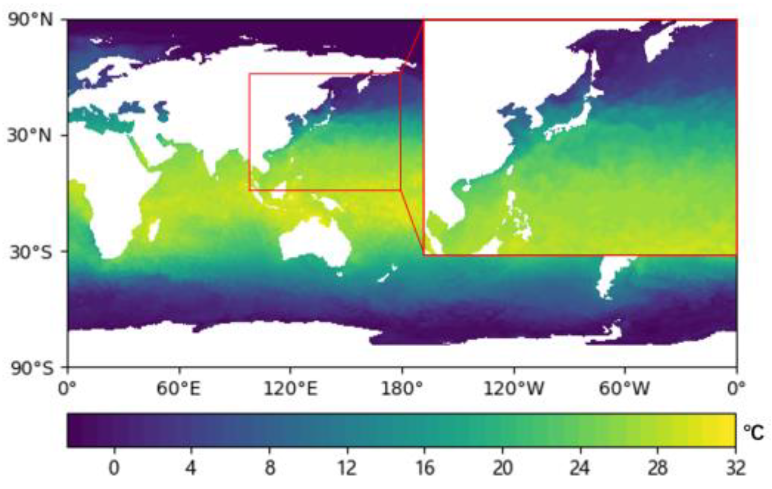
As shown in Figure 1, the study area is the Northwest Pacific, from 0° to 60°N and 100° to 180°E. The Northwest Pacific Ocean exhibits an intricate array of climate features, including tropical, subtropical, and temperate climates. The marine environment in this area is influenced by various natural factors, such as monsoons, ocean currents, and typhoons. Due to its diverse climate conditions and complex oceanic processes, this region is representative in SST prediction research.
The SST data used in this study is from the optimum interpolation sea surface temperature (OISST) v2.1 product, produced by the United States National Oceanic and Atmospheric Administration (NOAA), with a spatial resolution of 1/4° latitude by 1/4° longitude. The time scale of the predictions is daily, weekly, and monthly. The OISST for the study area covers temporal range from 1 January 1993 to 31 December 2020.
More information can be found at the following link: https://psl.noaa.gov/data/gridded/data.noaa.oisst.v2.highres.html, accessed on 11 May 2023.
2.2. Pre-Processing
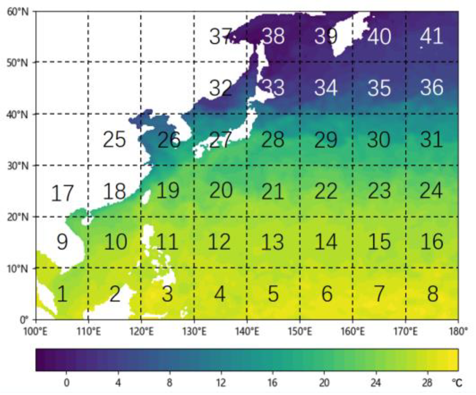
The data has a spatial resolution of 0.25°, with a corresponding grid size of 320 × 240 (8° × 6°) for the study area. Considering model parameter size, hardware and software environments, as well as the limited accuracy at large scales, we divide the study area into 8 × 6 subregions, each with a 40 × 40 (10° × 10°) grid. Subregions without ocean are excluded, leaving 41 subregions as experimental data, numbered sequentially (Figure 2).
Among the 41 subregions, 19 of them (1, 2, 3, 9, 10, 11, 17, 18, 19, 25, 26, 27, 28, 32, 33, 37, 38, 39, and 40) contain land or islands, forming incomplete sea areas. Therefore, the constructed subregion samples are representative.
Then, we divide the datasets into daily, weekly, and monthly mean. We allocate 60% of the data for training, 20% for testing, and 20% for validation to prevent overfitting. The specific time ranges for each set are presented in Table 1.
3. Methods
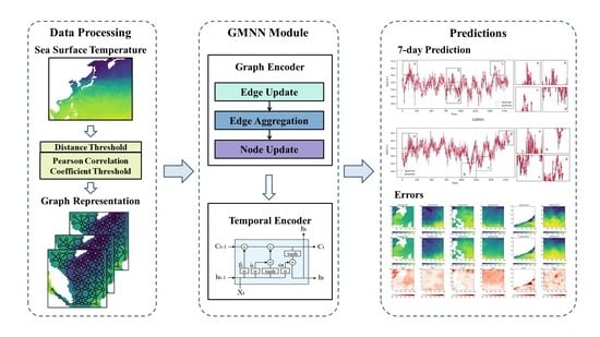
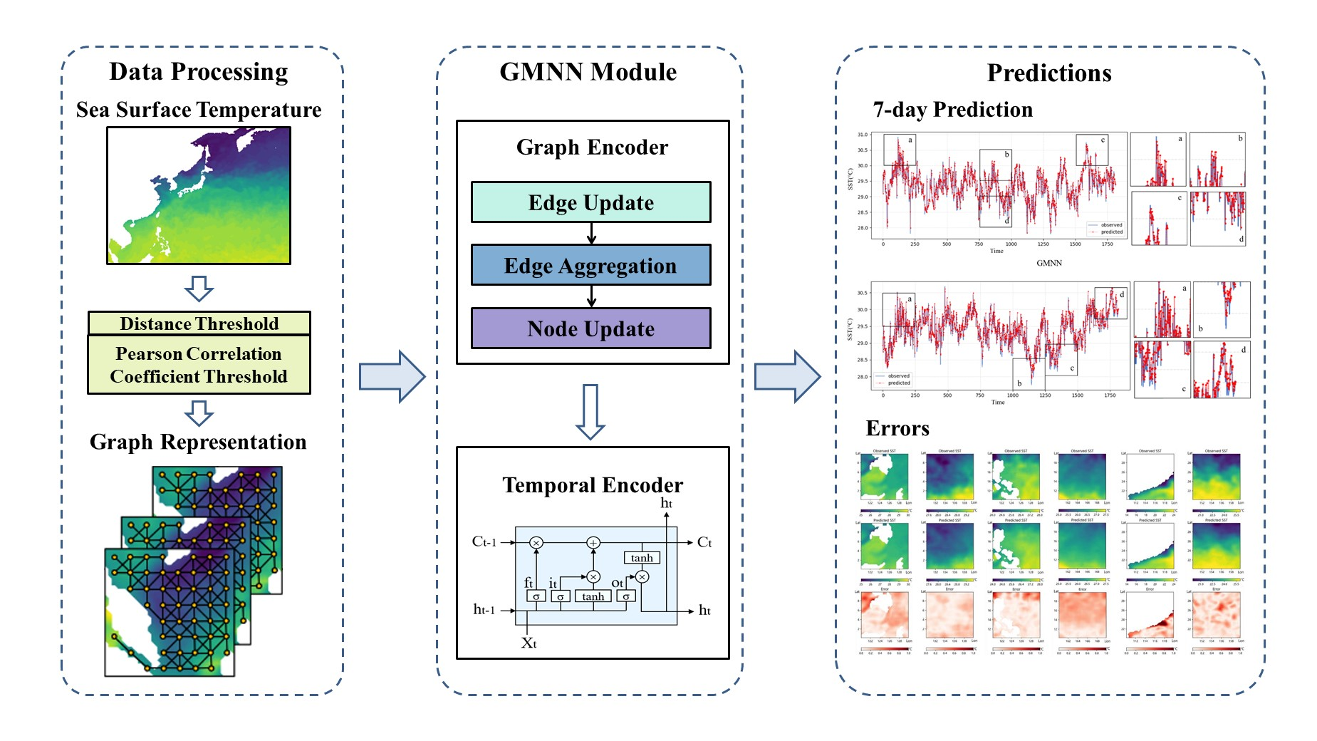
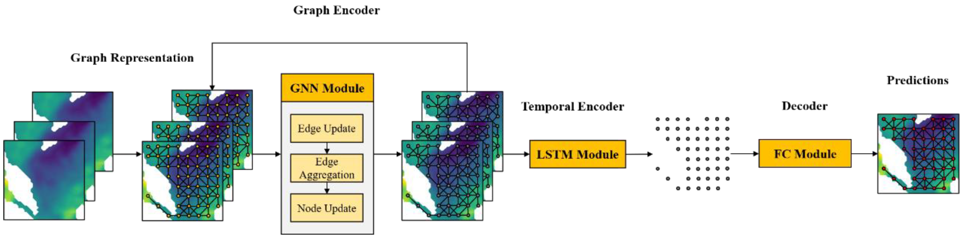
The complete framework of the graph memory neural network (GMNN) is presented in Figure 3. Initially, historical SST data are preprocessed and transformed into a series of time-sorted graphs with fixed time intervals. These graphs encompass temporal, spatial, and attribute features as the model input. Next, a neural network is constructed for the graph sequence, featuring an encoder with both graph and temporal encoder modules to learn spatial and temporal patterns. The graph encoder is composed of multiple iterative GNN layers, each aggregating and updating the graph’s nodes and edges to extract spatial features. The temporal encoder employs LSTM to capture temporal dynamics. Finally, by integrating the multi-output strategy and a fully connected layer decoder, the extracted spatiotemporal features are transformed into future SST prediction results.
3.1. Graph Representation
In research with defined coordinate systems, locations are represented by longitude and latitude pairs. For SST data, each point at the sea surface defined by a coordinate pair generates an SST record at each time step. Records from different locations form a spatially correlated snapshot, and a series of snapshots over time create a temporally connected sequence. An SST image sequence of length T can be denoted as .
In the study area with land and islands, some locations lack SST observations, leading to empty pixels. Consequently, each image in the time series contains valid pixels, where , and represent the number of rows and columns in the image, respectively.
To express the connectivity between pixels, we construct edges for each valid pixel based on distance threshold and Pearson correlation coefficient.
As shown in Equation (1), represents the connectivity between points and based on distance threshold, where 1 means connected and 0 means unconnected. represents the Euclidean distance between points and , with being the set distance threshold. When is greater than , the spatial association between points and is considered weak, and no edge is formed between them.
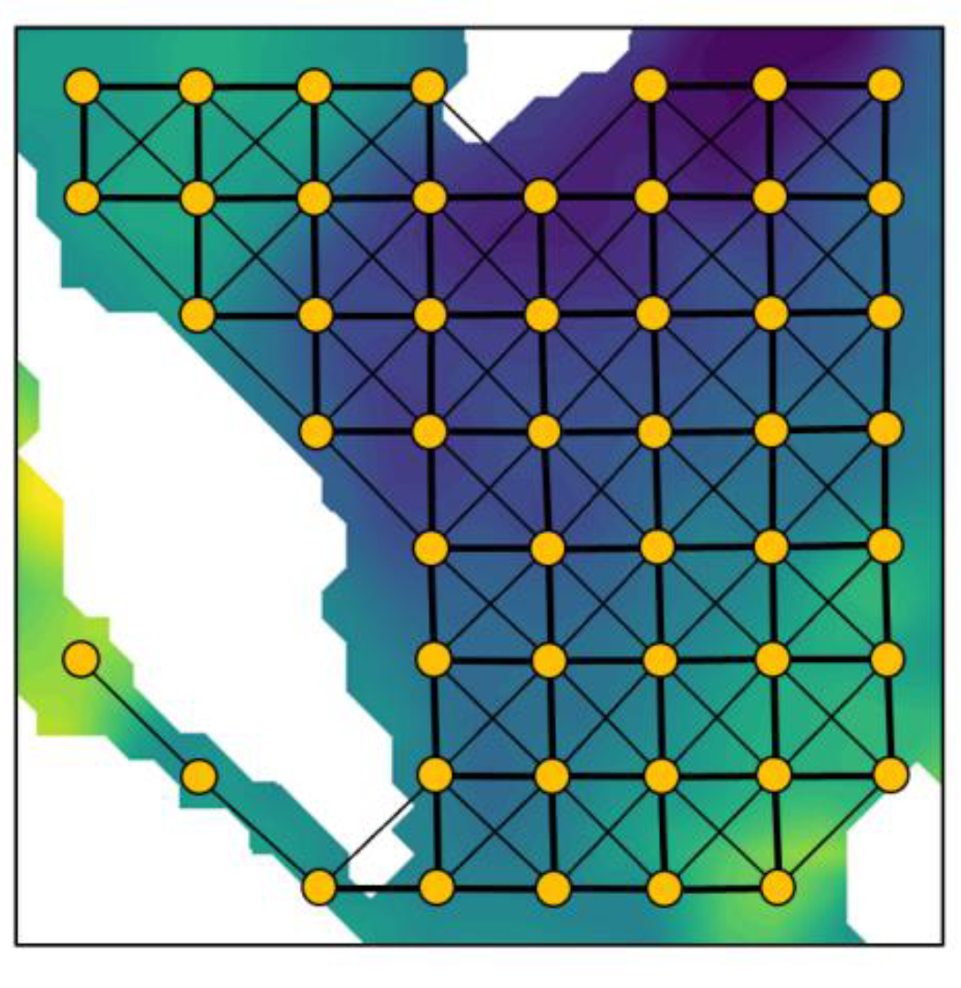
Figure 4 demonstrates the effect of edge construction based on distance threshold. Thicker solid lines represent edges with a distance threshold of 1, while thinner solid lines correspond to edges with a of .
The Pearson correlation coefficient (PCC) measures the linear relationship between two variables. Its value lies between −1 and 1, with larger absolute values indicating stronger correlations. The formula for the PCC, , is shown in Equation (2).
For SST prediction, and represent the SST value sets for points and on the sea surface, each containing samples corresponding to the time series length. and denote the SST values at time , and and are the average SST values of the two sets.
Equation (3) shows the edge construction based on the Pearson correlation coefficient, where represents the connectivity between points and based on Pearson correlation coefficient threshold, where 1 means connected and 0 means unconnected. is the threshold.
The distance threshold and Pearson correlation coefficient evaluate the spatial relationship between any two points on the graph from the perspectives of position relation and attribute correlation. By combining these two factors, we create an edge construction method, as shown in Equation (4).
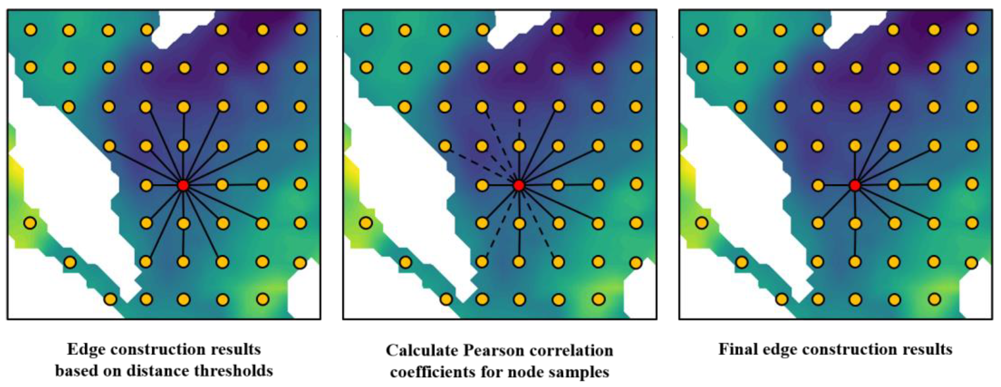
Figure 5 illustrates the edge construction process for a node in an SST image. The left image shows the edge connections when grid (grid equals 1/4°). Next, we calculate the Pearson correlation coefficient between the connected nodes, as depicted in the middle image. Solid lines represent calculations exceeding , while dashed lines represent calculations less than or equal to . By removing the dashed lines, we achieve the final result in the right image.
The values of and in our study are 1.5 grid and 0.8 grid, respectively. By applying the edge construction method to each node, we obtain the node and edge representation of SST data.
The SST image sequence is converted into a graph sequence . Each graph in the sequence is represented as a collection of nodes and edges connecting them, denoted as , where represents node , and represents the edge from to .
Compared to the pixel image representation, the graph representation offers greater flexibility, as it directly omits points corresponding to missing values.
3.2. Graph Encoder
GNN is a neural network that learns target objects by propagating neighbor information based on graph structures [36]. Compared to CNN, GNN excels at handling irregular data and is better suited for tasks with strong interdependencies [37,38], making them applicable for encoding SST variation process.
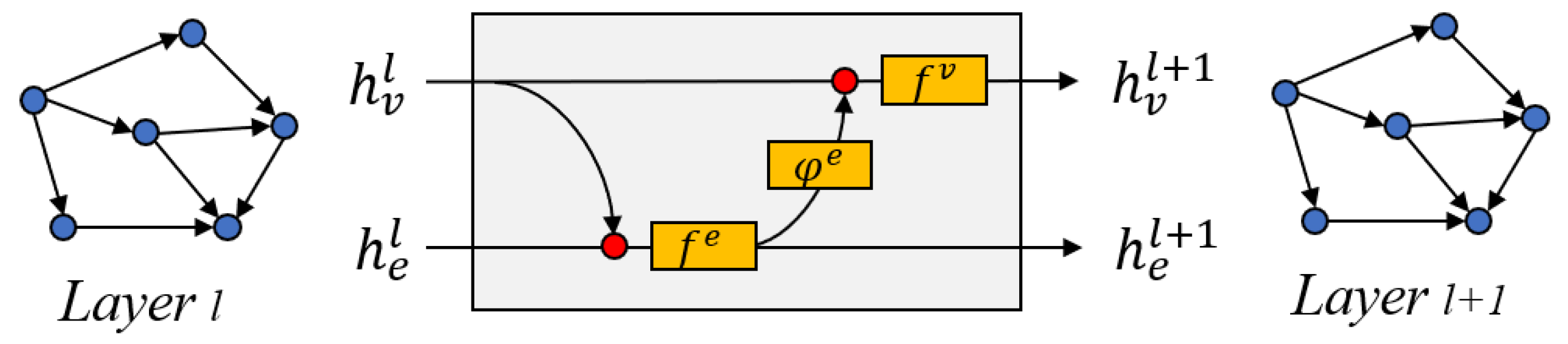
To incorporate features of nodes, edges, and their relationships, we adopt the multi-stage aggregation-update framework by Sanchez-Gonzalez et al. [39] and design a GNN module consisting of edge update, edge aggregation, and node update, as shown in Figure 6.
Here, is the aggregation function, designed to transfer edge states to nodes, thereby extracting more neighborhood information. is the update function, responsible for further updating the aggregated representations.
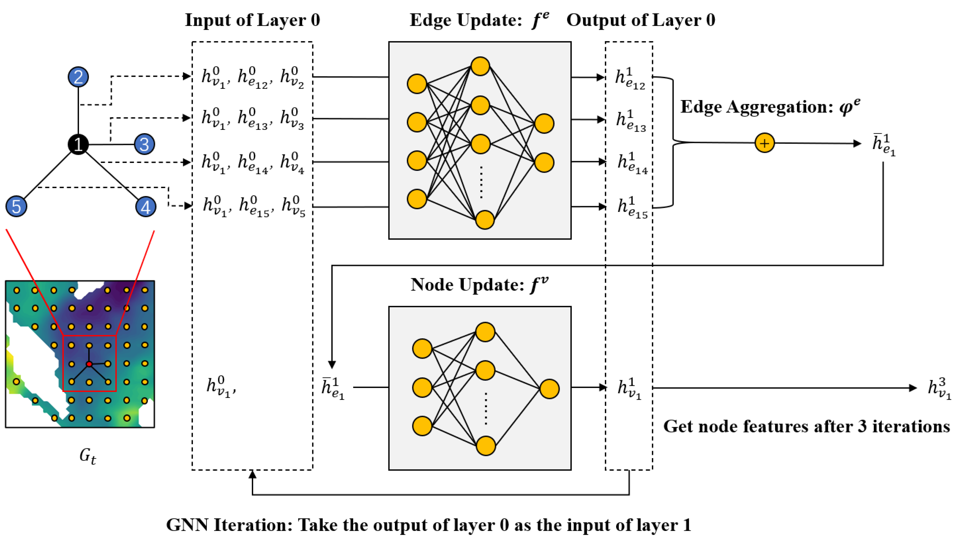
Then, we embed the GNN module into the model to form a graph encoder. Figure 7 displays its structure. The features shown are for a node and its neighborhood in the graph at time .
For graph , the node feature matrix is , with as the feature vector for node . The edge feature matrix is , and is the feature vector for edge . Here, is the number of nodes in , and denotes the number of edges. Node features have three dimensions, SST, longitude, and latitude. Edge features have two dimensions: direction and length, length represents the shortest path between two edges, and direction is a measure of its angle to the North. The hidden state of at layer is , and the hidden state of at layer is . Thus, the initial value is and .
- Edge update: As shown in Equation (5), we gather the current edge state and the states of its adjacent nodes, and pass them through the edge update function to obtain the updated result. This output will be used in the edge aggregation and the next iteration. The is a multilayer perceptron and a ReLU activation function to capture nonlinear features.
- Edge aggregation: Next, as shown in Equation (6), we use the function to aggregate the updated edge states of all connected edges for each node. Common aggregation methods include sum, mean, and max. Considering that for a point on the sea surface, heat changes manifest as a convergence or dissipation process, we choose the sum aggregation method.
- Node update: Finally, we gather the previous aggregation outputs and their current states and put them into the update function . Similar to , is also a combination of a multilayer perceptron and a ReLU activation function.
The three stages described above constitute a single iteration. By stacking multiple GNN layers and performing iterative updates, information can propagate within the graph, enabling the model to learn more abstract and complex features. In this study, we set the iteration times to 3.
3.3. Temporal Encoder
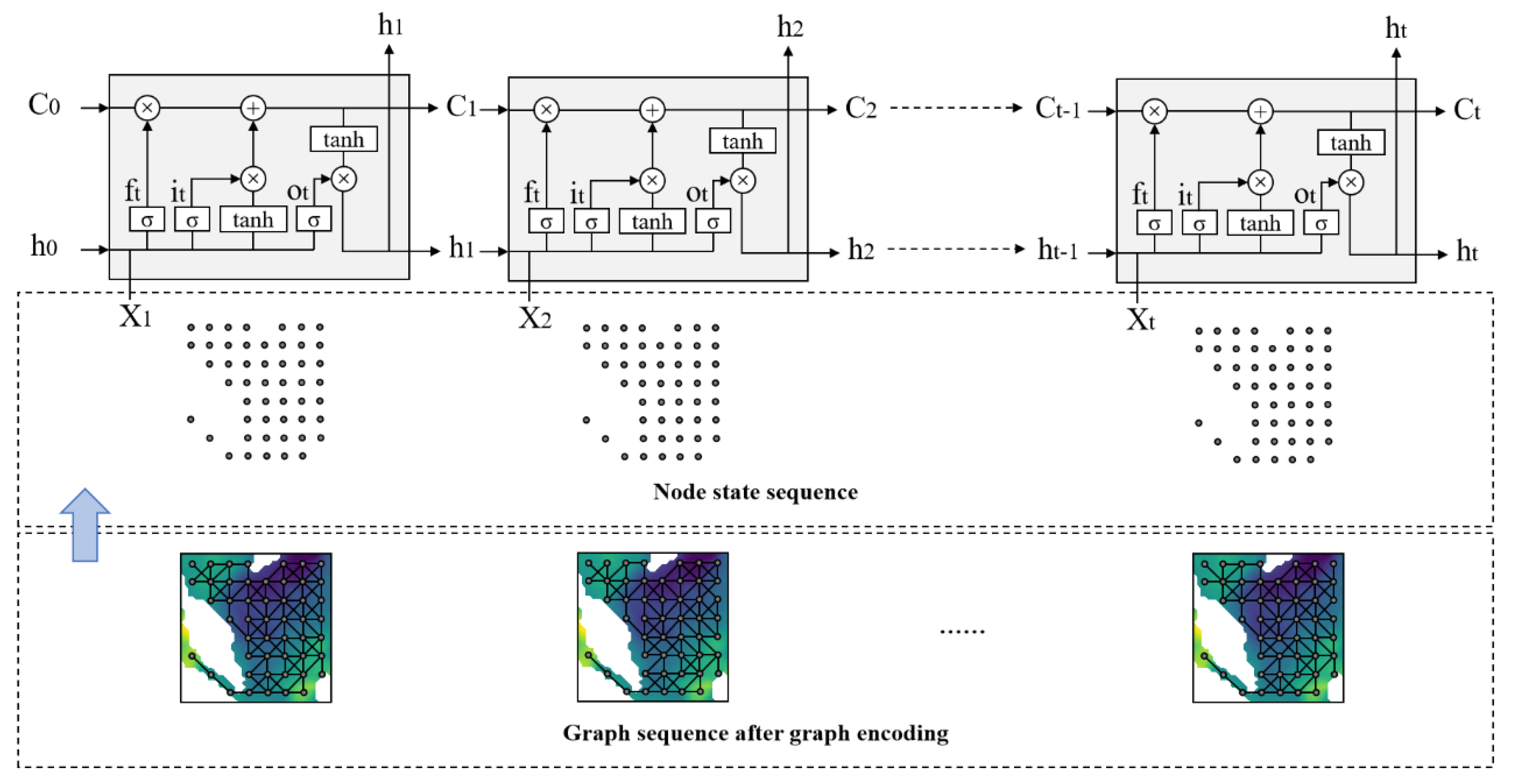
Figure 8 shows the structure and encoding process of the temporal encoder. A sequence of graphs with extracted spatial features is obtained after the graph encoder, which contains updated node and edge states. Then, we use the node state sequence as the input for the LSTM layer, and the encoded hidden state is acquired after temporal feature extraction.
The LSTM layer contains multiple LSTM units, which have the ability to selectively remember important information while filtering out noise [40]. This ability is attributed to the gating mechanism, which includes forget gate , input gate , and output gate , helps control gradients and addresses the vanishing and exploding gradient problems in RNNs.
3.4. Decoder and Loss Function
After the graph and temporal encoders, we obtain the node state . In this study, we aim to predict multi-step future SST values based on historical observations. Accordingly, we apply a direct multi-output prediction strategy to convert into a prediction sequence with a length equal to the prediction steps. The prediction steps are consistent with the time scale of the input data, for example, the time scale of the input data is daily, the prediction for each step is one day.
Then, we use the mean squared error (MSE) as the loss function in this study, as shown in Equation (8). denotes the total prediction steps, represents the actual value at time , and is the predicted value.
4. Experiments
4.1. Metrics
SST prediction is inherently a regression task. To accurately assess the performance of each model, we consider two perspectives: the deviation between predictions and observations, and data fitting. We choose three evaluation metrics: Root Mean Squared Error (RMSE), Mean Absolute Error (MAE), and R-squared. For a sequence of length , with as the observations at time and as the predictions, and as the average of observations, the formulas for each metric are provided below.
4.2. Compared Models
To evaluate the performance of GMNN, we selected three types of comparison models:
- FC-LSTM and FC-GRU: They are time series prediction models, which integrate LSTM or GRU layers with fully connected layers for feature extraction and improved representation capability.
- ConvLSTM: This is a spatiotemporal model utilizing CNN idea with LSTM, which incorporates convolution operations into input data and hidden states, allowing for the capture of spatial information and complex spatiotemporal features.
- GCN-LSTM: This is a spatiotemporal model employing GNN idea, which combines graph convolutional networks (GCN) with LSTM for graph sequence prediction, effectively extracting features from nodes and their multi-order neighbors and integrating them into the LSTM layer for temporal information processing.
4.3. Results of Different Subregions
To verify the generalization ability of GMNN in different regions, we select several subregions in the daily mean dataset and predict the SST for the next 1, 3, and 7 days.
GMNN is applicable to both complete and incomplete sea areas (with land or islands). In contrast, ConvLSTM based on CNN idea, is suitable only for complete sea areas, the missing values in incomplete sea areas must be filled using interpolation, which introduces noise and can affect model accuracy. Therefore, we select data from three incomplete sea area subregions (No. 1, 2, and 3) and three complete sea area subregions (No. 4, 5, and 6) at the same latitude for comparison (Figure 2). The models for incomplete sea area subregions include FC-LSTM, FC-GRU, and GCN-LSTM. For complete sea area subregions, FC-LSTM, FC-GRU, ConvLSTM, and GCN-LSTM are used.
4.3.1. Results of Incomplete Sea Areas
We analyze the effectiveness of our model in incomplete sea areas, taking subregion 1 as an example. The constructed graph in this region contains 1245 nodes. Table 2 shows the experiment results.
The two worst-performing models are FC-LSTM and FC-GRU, with the maximum RMSE, MAE and the minimum R- squared (Table 2), indicating that ignoring spatial correlation can significantly affect prediction accuracy. There is little difference between these two models and FC-GRU’s is slightly worse than FC-LSTM’s when predicting the future 3 and 7 days. This suggests that in this study, using LSTM for time feature extraction is more suitable. Both graph-based models exhibit good performance, with GMNN performing the best in all metrics. For instance, in terms of RMSE for seven-day prediction, GMNN’s 0.288 is 7.7% lower than FC-LSTM and 1.6% lower than GCN-LSTM. This indicates that the iterative GNN idea can effectively capture the spatial information of SST data.
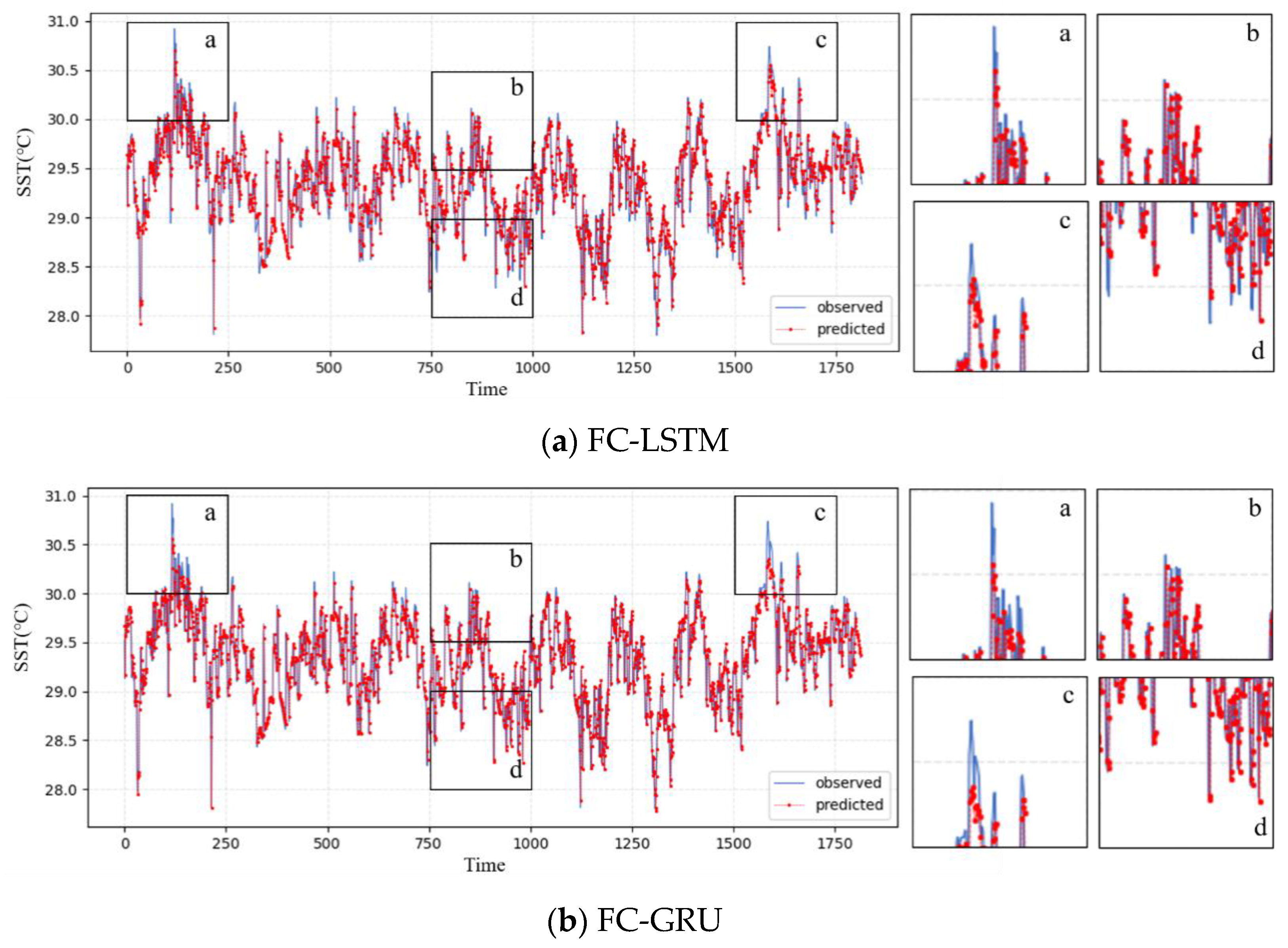
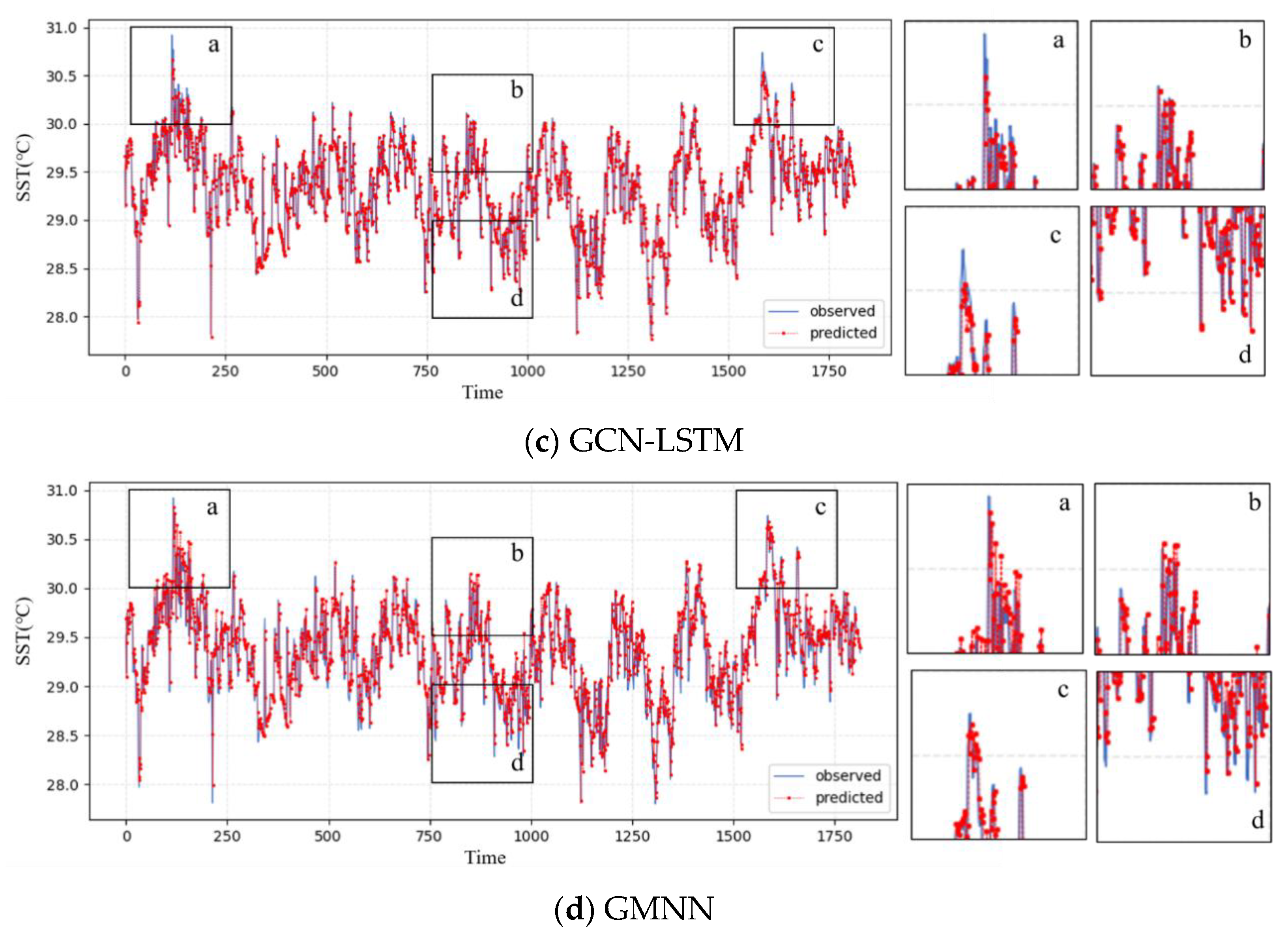
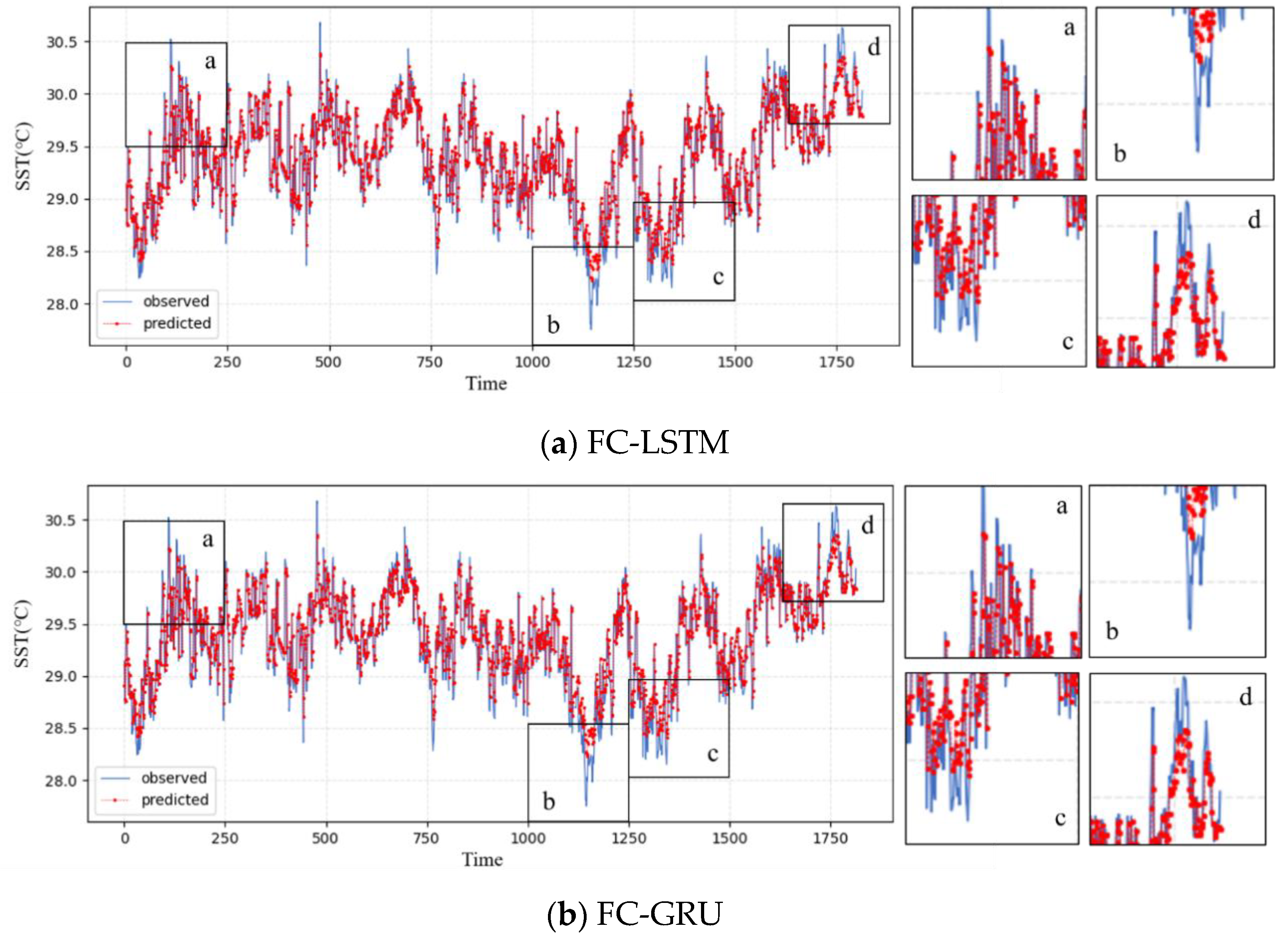
To visually compare the results, we take the node with longitude 109.875°E and latitude 0.125°N in subregion 1 as an example. The predictions and observations of each model were compared using a line chart for a 7-step prediction, as shown in Figure 9.
It can be seen that the main difference in the prediction results of each model lies in the degree of fitting to the peak values. Therefore, we select four peak areas, a, b, c, and d for detailed analysis. Among them, a and c are steep peak areas, while b is a gentle peak area, and d is a low peak area.
FC-GRU predicts well in b and d, but has the worst performance among all models in the steep peak areas a and c. FC-LSTM performs slightly better than FC-GRU in the steep peak areas, but its fitting degree in the low peak area is low. GCN-LSTM’s predictions can already fit the observations well, but there is still room for improvement in the steep peak areas. GMNN has the best overall prediction accuracy, showing a high degree of fitting in these peak areas with different characteristics. Especially in the steep peak areas, the performance is significantly better than the other compared models.
4.3.2. Results of Complete Sea Areas
Similarly, we analyze the effectiveness of GMNN in complete sea areas using the example of subregion 4 which contains 1600 nodes. The results are shown in Table 3.
FC-LSTM and FC-GR performed the worst. ConvLSTM which uses CNN idea, exhibits good performance in complete sea areas where data can be expressed in pixel form, and its prediction accuracy is slightly better than that of the GCN-LSTM model, which uses graph idea. Among prediction models, GMNN is better than other models in the metrics. GMNN’s RMSE value for seven-day prediction decreased by 5.5% compared to FC-LSTM, 0.9% compared to ConvLSTM, and 2.0% compared to GCN-LSTM.
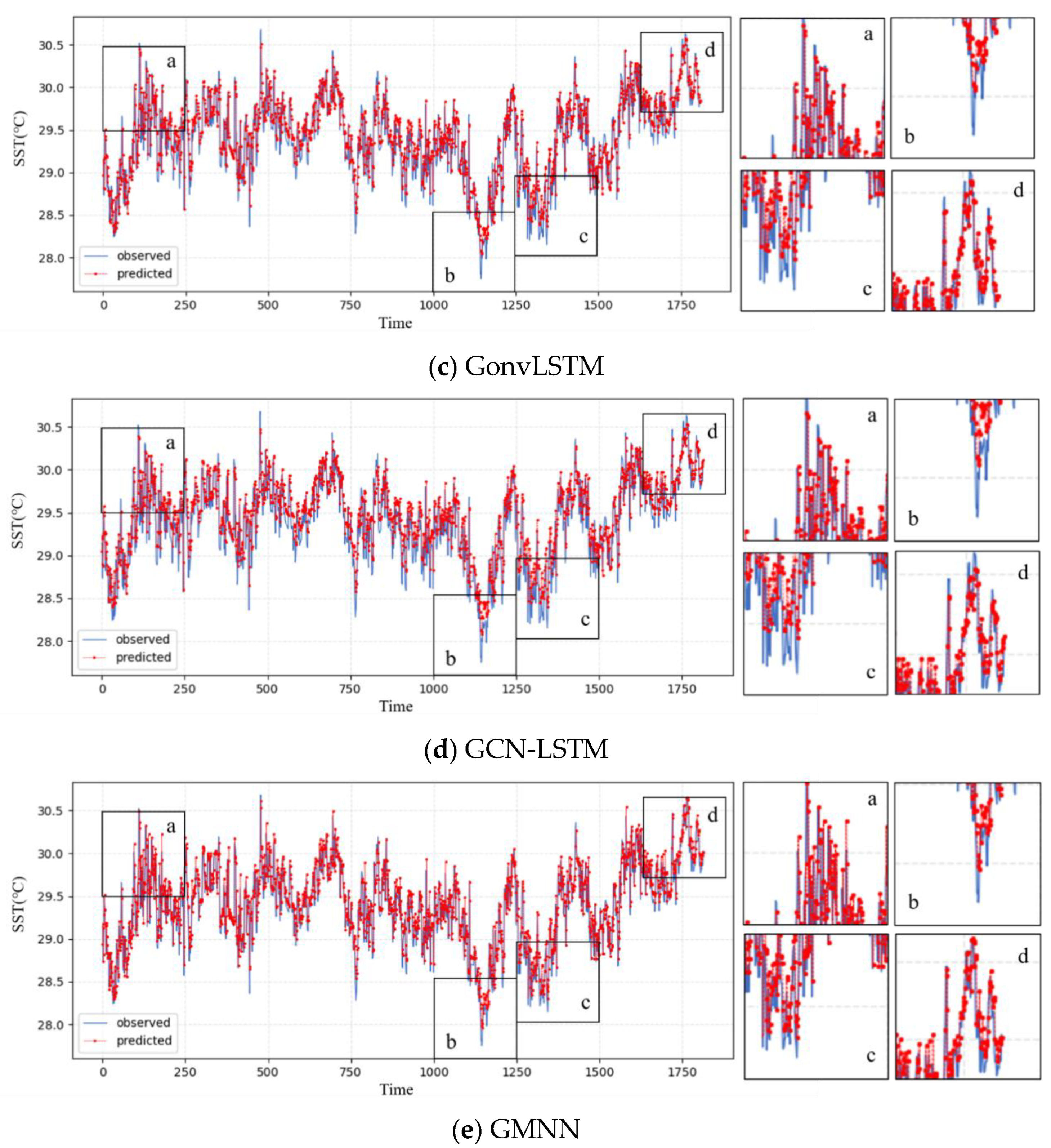
As shown in Figure 10, a comparison chart of the seven-day predictions and observations is created for node located at 130.125°E and 0.125°N in subregion 4. We analyze two high peaks (a, d) and two low peaks (b, c) in detail. The performance of FC-LSTM and FC-GRU is quite similar, with poor predictions for the highest and lowest points in all four areas. ConvLSTM and GCN-LSTM show significant improvement in the prediction of areas a, b, and d, with ConvLSTM showing better fitting. GMNN performs well in all four areas with excellent prediction ability.
The results prove that GMNN has excellent prediction ability in both complete and incomplete sea areas.
4.4. Results of Different Time Scales
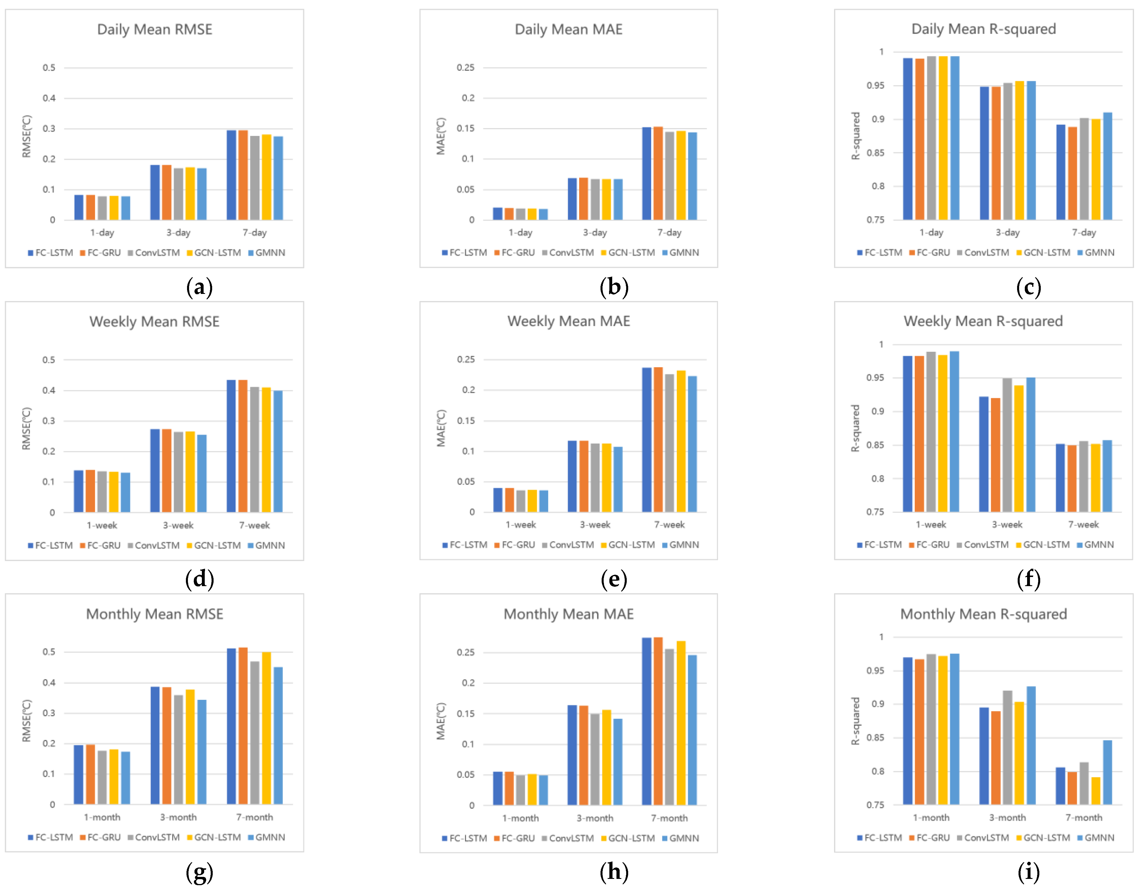
To verify the accuracy and stability of GMNN for different time scales and prediction steps, we conduct comparison experiments for future 1 step, 3 steps, and 7 steps on three types of datasets: daily, weekly, and monthly mean, using the example of subregion 5. The results are presented in Figure 11. The y-axis of each metric is standardized across different time scales for comparison.
From the perspective of fixed time scales, as the prediction step increases, the performance of each model declines, with RMSE and MAE increasing and R-squared decreasing. Taking daily predictions as an example, the R-squared, RMSE, and MAE for predicting one day ahead are 0.994, 0.078, and 0.018, respectively. When predicting three days ahead, R-squared decreased by 0.037, while RMSE and MAE both increased by more than double. When predicting seven days ahead, R-squared continued to decrease by 0.047, with RMSE and MAE increasing by 0.62 and 1.10 times, respectively. This suggests that multi-step prediction incurs greater errors than single-step prediction. With an increasing number of prediction steps, more relationships need to be learned, and models become more challenged in capturing the changing trends and periodicity of time series, which results in increased errors.
From the perspective of fixed prediction steps, as the time scale increases, the performance of each model also declines. Taking RMSE as an example, on a daily scale, the RMSE is 0.078, 0.170, and 0.275, when predicting the future 1, 3, and 7 step. On a weekly scale, the RMSE increases by 0.67 times, 0.50 times, and 0.46 times when predicting 1, 3, and 7 steps in the future. On a monthly scale, compared with the weekly scale, the RMSE increases by 0.33 times, 0.34 times, and 0.13 times when predicting 1, 3, and 7 steps in the future. The reasons for this phenomenon are mainly twofold. First, the time series of daily, weekly, and monthly mean datasets used in this study contain 10,227, 1461, and 336 time steps, respectively, which means that the data available for training are sparser at larger time scales, and affect the prediction accuracy. Second, from daily to weekly to monthly, the smoothness of the SST changes gradually decreases, and the changing trend and periodicity of the time series become less obvious, making it difficult to capture the nonlinear features, resulting in a decrease in prediction accuracy.
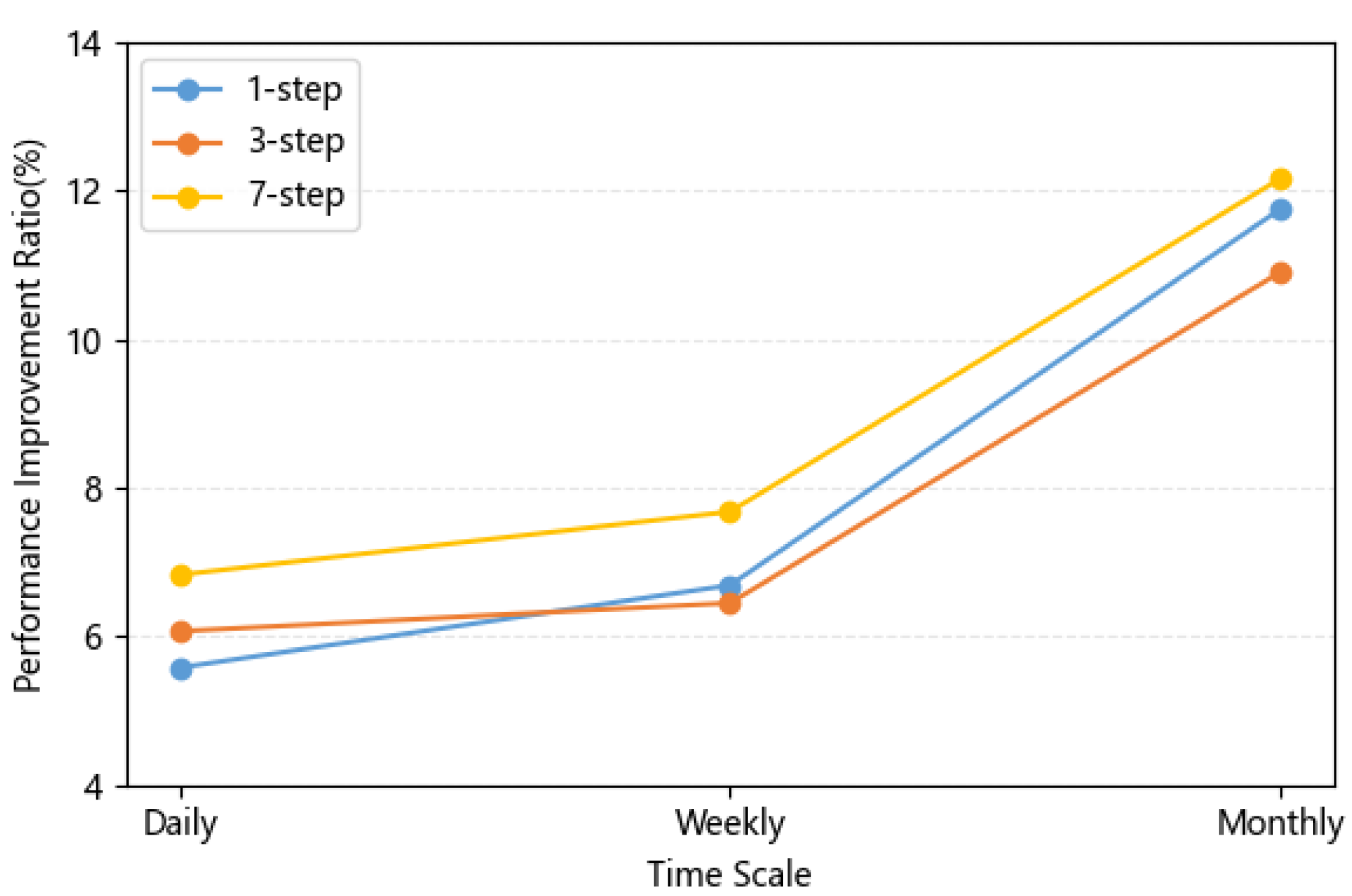
As shown in Figure 11, GMNN has better prediction accuracy than the comparison models at different time scales and prediction steps. In order to more clearly show the performance improvement, we use FC-LSTM as the baseline and calculate the percentage of RMSE reduction of GMNN relative to the baseline under different time scales and prediction steps (Figure 12), which serves as the performance improvement ratio.
At the same time scale, changes in the prediction step do not result in significant changes in the improvement ratio. However, when the time scale changes to the monthly scale at the same prediction step, the improvement ratio increases significantly. This suggests that GMNN can capture hidden spatiotemporal features on large scales.
5. Discussion
5.1. Model Comparison
Through experiments in different partitions, time scales, and prediction steps, we find that our GMNN is better than other comparison models, which can be categorized into time series models (FC-LSTM, FC-GRU), convolution-based model (ConvLSTM), and graph-based model (GCN-LSTM). The results provide insights into the applicability and effectiveness of different ideas for SST prediction tasks.
The inferior performance of time series models suggests the impact of neglecting spatial information on prediction accuracy. Convolution-based models and graph-based models differ in their learning styles and applicable structures. In terms of learning styles, CNN extracts feature by sliding convolution kernels, thus exhibiting strong capabilities in extracting multi-scale local spatial features [41]. GNN focus more on adjacency relationships, with their message-passing mechanism providing better abilities for tasks with strong object interrelations. As SST is influenced by ocean currents, winds, and heat exchange processes in nearby regions, graph-based models can well represent temperature variation processes. Regarding applicable structures, CNN is based on traditional grid structures and is suitable for regular datasets. Therefore, convolution-based model (ConvLSTM) demonstrates excellent forecasting performance in experiments with complete sea area datasets. Graph-based models, on the other hand, are not restricted by data regularity, offering greater flexibility.
Both being graph-based methods, the iterative GNN used in this study and the GCN adopted by the comparison model GCN-LSTM differ in the information they emphasize. GCN primarily focuses on node information, with its convolution operation aggregating features of nodes and their adjacent counterparts [42,43]. Although GCN considers node information and adjacency relationships, edge attributes are typically not directly incorporated into calculations. In contrast, the iterative GNN takes both node and edge information into account through its designed aggregation and update functions. As a result, in comparative experiments, GMNN consistently achieves better prediction outcomes than GCN-LSTM.
5.2. Error Distribution
To clearly show the prediction performance and error distribution of our model, we use the future seven-day prediction results of GMNN and select 12 subregions with observations, predictions, and errors on 26 February 2016 for analysis. Among them, two regions are selected within every 10° latitude range, corresponding to incomplete and complete sea areas, respectively. The experiment results of the 12 regions are shown in Figure S1.
When comparing the error between two regions at the same latitude, there is no significant difference in the prediction accuracy of the model between incomplete and complete sea areas, indicating a good prediction performance in both types of regions.
Comparing the errors of regions at different latitudes, the regions with latitudes between 30°N and 50°N have the largest errors, followed by the regions between 20°N and 30°N and between 50°N and 60°N, while the regions between 0°–20°N have relatively smaller errors. The complexity of the meteorological and oceanic environment is the main reason for the differences in the prediction performance among these regions. Regions between 30° and 50°N belong to the North Temperate Zone and are influenced by subtropical high-pressure zones, westerlies, monsoons, and continental climates. They are also affected by multiple ocean currents such as the Kuroshio Current, the Oyashio Current, and the North Pacific Warm Current, resulting in complex spatiotemporal characteristics and making predictions difficult. In contrast, regions between 0° and 20°N are mainly affected by tropical and subtropical climates, with relatively simple spatiotemporal characteristics and thus easier to predict. Regions between 20° and 30°N and between 50° 60°N have moderate environmental complexity and prediction difficulty.
6. Conclusions
In this paper, we propose a GMNN to predict future SST. The model uses a graph representation method based on distance threshold and Pearson correlation coefficient to transform SST data into a graph structure, thus overcoming the limitations of convolution-based methods in encoding irregular data that includes land or islands. We also design a graph encoder based on iterative GNN, incorporating edge information to fully express the heat transfer process at the sea surface. To validate the effectiveness of GMNN, we choose time series prediction models (FC-LSTM, FC-GRU), convolution-based model (ConvLSTM), and graph-based model without considering edge information (GCN-LSTM) as comparison. We conduct experiments of these models in incomplete and complete sea area partitions, daily, weekly and monthly time scales, as well as 1-step, 3-step, and 7-step prediction steps, and our model exhibits superior prediction ability compared to the others, reflecting its accuracy and stability.
In addition, we find that with increasing time scales and prediction steps, the prediction accuracy decreases. GMNN shows a higher performance improvement at the monthly time scale than at the daily and weekly time scales. Error analysis reveals that GMNN has larger prediction errors for areas with greater temperature variations. The errors also have a certain correlation with latitude, with higher errors for the region of 30–50°N due to the complex ocean and meteorological environment, and lower errors for the region of 0–20°N with relatively stable temperature changes.
However, there are still some limitations in our work. Although we use SST as the input for prediction, in the future, other factors will be considered and collected for systematic analysis so as to explore the impact of these factors on SST prediction. Moreover, the study area in this case was the Northwest Pacific. To generalize the ability of our model, we will select different ocean basins with various dynamic features and make improvements in subsequent studies to explore large-scale SST prediction.
Supplementary Materials
The following supporting information can be downloaded at: https://www.mdpi.com/article/10.3390/rs15143539/s1, Figure S1: GMNN prediction results for SST on 26 February 2016, in 12 subregions: (a) Subregion 3; (b) Subregion 4; (c) Subregion 11; (d) Subregion 15; (e) Subregion 18; (f) Subregion 22; (g) Subregion 27; (h) Subregion 30; (i) Subregion 32; (j) Subregion 36; (k) Subregion 40; (l) Subregion 41.
Author Contributions
Conceptualization, L.H.; Data curation, L.H.; Formal analysis, M.Q.; Funding acquisition, Z.D. and R.L.; Methodology, M.Q.; Project administration, Z.D. and R.L.; Resources, Z.D. and R.L.; Software, S.L. and A.Z.; Supervision, L.H. and S.W.; Validation, S.W.; Visualization, S.L. and A.Z.; Writing—original draft, S.L.; Writing—review & editing, A.Z., M.Q. and S.W. All authors have read and agreed to the published version of the manuscript.
Funding
This research was supported by the National Natural Science Foundation of China (42225605) and China Postdoctoral Science Foundation (2022M720121).
Data Availability Statement
Publicly available datasets were analyzed in this study. The SST data can be downloaded from https://psl.noaa.gov/data/gridded/data.noaa.oisst.v2.highres.html, accessed on 11 May 2023.
Conflicts of Interest
The authors declare no conflict of interest.
References
- Wang, G.; Cheng, L.; Abraham, J.; Li, C. Consensuses and discrepancies of basin-scale ocean heat content changes in different ocean analyses. Clim. Dyn. 2018, 50, 2471–2487. [Google Scholar] [CrossRef] [Green Version]
- Ham, Y.; Kug, J.; Park, J.; Jin, F. Sea surface temperature in the north tropical Atlantic as a trigger for El Niño/Southern Oscillation events. Nat. Geosci. 2013, 6, 112–116. [Google Scholar] [CrossRef]
- Chen, Z.; Wen, Z.; Wu, R.; Lin, X.; Wang, J. Relative importance of tropical SST anomalies in maintaining the Western North Pacific anomalous anticyclone during El Niño to La Niña transition years. Clim. Dyn. 2016, 46, 1027–1041. [Google Scholar] [CrossRef]
- Andrade, H.A.; Garcia, C.A.E. Skipjack tuna fishery in relation to sea surface temperature off the southern Brazilian coast. Fish Oceanogr. 1999, 8, 245–254. [Google Scholar] [CrossRef]
- Wang, W.; Zhou, C.; Shao, Q.; Mulla, D.J. Remote sensing of sea surface temperature and chlorophyll-a: Implications for squid fisheries in the north-west Pacific Ocean. Int. J. Remote Sens. 2010, 31, 4515–4530. [Google Scholar] [CrossRef]
- Khan, T.M.A.; Singh, O.P.; Rahman, M.S. Recent sea level and sea surface temperature trends along the Bangladesh coast in relation to the frequency of intense cyclones. Mar. Geod. 2000, 23, 103–116. [Google Scholar] [CrossRef]
- Emanuel, K.; Sobel, A. Response of tropical sea surface temperature, precipitation, and tropical cyclone-related variables to changes in global and local forcing. J. Adv. Model. Earth Syst. 2013, 5, 447–458. [Google Scholar] [CrossRef]
- Chassignet, E.P.; Hurlbert, H.E.; Smedstad, O.M.; Halliwell, G.R.; Hogan, P.J.; Wallcraft, A.J.; Bleck, R. Ocean prediction with the hybrid coordinate ocean model (HYCOM). In Ocean Weather Forecasting: An Integrated View of Oceanography; Springer: Berlin/Heidelberg, Germany, 2006; pp. 413–426. [Google Scholar] [CrossRef]
- Chassignet, E.P.; Hurlburt, H.E.; Metzger, E.J.; Smedstad, O.M.; Cummings, J.A.; Halliwell, G.R. US GODAE: Global ocean prediction with the HYbrid Coordinate Ocean Model (HYCOM). Oceanography 2009, 22, 64–75. [Google Scholar] [CrossRef] [Green Version]
- Qian, C.; Huang, B.; Yang, X.; Chen, G. Data science for oceanography: From small data to big data. Big Earth Data 2022, 6, 236–250. [Google Scholar] [CrossRef]
- Kartal, S. Assessment of the spatiotemporal prediction capabilities of machine learning algorithms on Sea Surface Temperature data: A comprehensive study. Eng. Appl. Artif. Intell. 2023, 118, 105675. [Google Scholar] [CrossRef]
- Xue, Y.; Leetmaa, A. Forecasts of Tropical Pacific SST and Sea Level Using a Markov Model. Geophys. Res. Lett. 2000, 27, 2701–2704. [Google Scholar] [CrossRef] [Green Version]
- Collins, D.C.; Reason, C.J.C. Predictability of Indian Ocean Sea Surface Temperature Using Canonical Correlation Analysis. Clim. Dyn. 2004, 22, 481–497. [Google Scholar] [CrossRef]
- Neetu, S.R.; Basu, S.; Sarkar, A.; Pal, P.K. Data-Adaptive Prediction of Sea-Surface Temperature in the Arabian Sea. Ieee Geosci. Remote Sens. Lett. 2010, 8, 9–13. [Google Scholar] [CrossRef]
- Shao, Q.; Li, W.; Han, G.; Hou, G.; Liu, S.; Gong, Y.; Qu, P. A Deep Learning Model for Forecasting Sea Surface Height Anomalies and Temperatures in the South China Sea. J. Geophys. Res. Ocean. 2021, 126, e2021JC017515. [Google Scholar] [CrossRef]
- Garcia-Gorriz, E.; Garcia-Sanchez, J. Prediction of Sea Surface Temperatures in the Western Mediterranean Sea by Neural Networks Using Satellite Observations. Geophys. Res. Lett. 2007, 34. [Google Scholar] [CrossRef]
- Lee, Y.; Ho, C.; Su, F.; Kuo, N.; Cheng, Y. The Use of Neural Networks in Identifying Error Sources in Satellite-Derived Tropical SST Estimates. Sensors 2011, 11, 7530–7544. [Google Scholar] [CrossRef]
- Lins, I.D.; Araujo, M.; Moura, M.D.C.; Silva, M.A.; Droguett, E.L. Prediction of Sea Surface Temperature in the Tropical Atlantic by Support Vector Machines. Comput. Stat. Data Anal. 2013, 61, 187–198. [Google Scholar] [CrossRef]
- Zhang, Q.; Wang, H.; Dong, J.; Zhong, G.; Sun, X. Prediction of Sea Surface Temperature Using Long Short-Term Memory. IEEE Geosci. Remote Sens. Lett. 2017, 14, 1745–1749. [Google Scholar] [CrossRef] [Green Version]
- Sun, T.; Feng, Y.; Li, C.; Zhang, X. High Precision Sea Surface Temperature Prediction of Long Period and Large Area in the Indian Ocean Based on the Temporal Convolutional Network and Internet of Things. Sensors 2022, 22, 1636. [Google Scholar] [CrossRef]
- Su, H.; Zhang, T.; Lin, M.; Lu, W.; Yan, X. Predicting subsurface thermohaline structure from remote sensing data based on long short-term memory neural networks. Remote Sens. Environ. 2021, 260, 112465. [Google Scholar] [CrossRef]
- Guo, H.; Xie, C. Multi-Feature Attention Based LSTM Network for Sea Surface Temperature Prediction. In Proceedings of the 3rd International Conference on Computer Information and Big Data Applications, Wuhan, China, 25–27 March 2022. [Google Scholar]
- Yang, Y.; Dong, J.; Sun, X.; Lima, E.; Mu, Q.; Wang, X. A CFCC-LSTM Model for Sea Surface Temperature Prediction. IEEE Geosci. Remote Sens. Lett. 2018, 15, 207–211. [Google Scholar] [CrossRef]
- Yu, X.; Shi, S.; Xu, L.; Liu, Y.; Miao, Q.; Sun, M. A Novel Method for Sea Surface Temperature Prediction Based on Deep Learning. Math. Probl. Eng. 2020, 2020, 6387173. [Google Scholar] [CrossRef]
- Qiao, B.; Wu, Z.; Tang, Z.; Wu, G. Sea Surface Temperature Prediction Approach Based on 3D CNN and LSTM with Attention Mechanism. In Proceedings of the 23rd International Conference on Advanced Communication Technology (ICACT), PyeongChang, Republic of Korea, 7–10 February 2021. [Google Scholar] [CrossRef]
- Shi, X.; Chen, Z.; Wang, H.; Yeung, D.; Wong, W. Convolutional LSTM Network: A Machine Learning Approach for Precipitation Nowcasting. Adv. Neural Inf. Process. Syst. 2015, 28, 1–9. [Google Scholar] [CrossRef]
- Xiao, C.; Chen, N.; Hu, C.; Wang, K.; Xu, Z.; Cai, Y.; Xu, L.; Chen, Z.; Gong, J. A spatiotemporal deep learning model for sea surface temperature field prediction using time-series satellite data. Environ. Modell. Softw. 2019, 120, 104502. [Google Scholar] [CrossRef]
- Jung, S.; Kim, Y.J.; Park, S.; Im, J. Prediction of Sea Surface Temperature and Detection of Ocean Heat Wave in the South Sea of Korea Using Time-series Deep-learning Approaches. Korean J. Remote Sens. 2020, 36, 1077–1093. [Google Scholar] [CrossRef]
- Zhang, K.; Geng, X.; Yan, X.H. Prediction of 3-D Ocean Temperature by Multilayer Convolutional LSTM. IEEE Geosci. Remote Sens. Lett. 2020, 17, 1303–1307. [Google Scholar] [CrossRef]
- Zhang, X.; Li, Y.; Frery, A.C.; Ren, P. Sea Surface Temperature Prediction With Memory Graph Convolutional Networks. IEEE Geosci. Remote Sens. Lett. 2022, 19, 1–5. [Google Scholar] [CrossRef]
- Zhou, J.; Cui, G.; Hu, S.; Zhang, Z.; Yang, C.; Liu, Z.; Wang, L.; Li, C.; Sun, M. Graph neural networks: A review of methods and applications. AI Open 2020, 1, 57–81. [Google Scholar] [CrossRef]
- Gilmer, J.; Schoenholz, S.S.; Riley, P.F.; Vinyals, O.; Dahl, G.E. Neural Message Passing for Quantum Chemistry. arXiv 2017, arXiv:1704.01212. [Google Scholar] [CrossRef]
- Sun, Y.; Yao, X.; Bi, X.; Huang, X.; Zhao, X.; Qiao, B. Time-Series Graph Network for Sea Surface Temperature Prediction. Big Data Res. 2021, 25, 100237. [Google Scholar] [CrossRef]
- Wang, T.; Li, Z.; Geng, X.; Jin, B.; Xu, L. Time Series Prediction of Sea Surface Temperature Based on an Adaptive Graph Learning Neural Model. Future Internet 2022, 14, 171. [Google Scholar] [CrossRef]
- Pan, J.; Li, Z.; Shi, S.; Xu, L.; Yu, J.; Wu, X. Adaptive graph neural network based South China Sea seawater temperature prediction and multivariate uncertainty correlation analysis. Stoch. Environ. Res. Risk Assess. 2022, 37, 1877–1896. [Google Scholar] [CrossRef]
- Xia, F.; Sun, K.; Yu, S.; Aziz, A.; Wan, L.; Pan, S.; Liu, H. Graph Learning: A Survey. IEEE Trans. Artif. Intell. 2021, 2, 109–127. [Google Scholar] [CrossRef]
- LeCun, Y.; Bengio, Y. Convolutional Networks for Images, Speech, and Time-Series. In The Handbook of Brain Theory and Neural Networks; MIT Press: Cambridge, MA, USA, 1995; pp. 255–258. [Google Scholar]
- Ye, Z.; Kumar, Y.J.; Sing, G.O.; Song, F.; Wang, J. A Comprehensive Survey on Graph Neural Networks for Knowledge Graphs. IEEE Access 2019, 10, 75729–75741. [Google Scholar] [CrossRef]
- Scarselli, F.; Gori, M.; Tsoi, A.; Hagenbuchner, M.; Monfardini, G. The Graph Neural Network Model. IEEE Trans. Neural Netw. 2009, 20, 61–80. [Google Scholar] [CrossRef] [PubMed] [Green Version]
- Hochreiter, S.; Schmidhuber, J. Long Short-Term Memory. Neural Comput. 1997, 9, 1735–1780. [Google Scholar] [CrossRef]
- Li, Z.; Liu, F.; Yang, W.; Peng, S.; Zhou, J. A Survey of Convolutional Neural Networks: Analysis, Applications, and Prospects. IEEE Trans. Neural Netw. Learn. Syst. 2022, 33, 6999–7019. [Google Scholar] [CrossRef]
- Bruna, J.; Zaremba, W.; Szlam, A.; LeCun, Y. Spectral Networks and Deep Locally Connected Networks on Graphs. arXiv 2014, arXiv:1312.6203. [Google Scholar] [CrossRef]
- Micheli, A. Neural Network for Graphs: A Contextual Constructive Approach. IEEE Trans. Neural Netw. 2009, 20, 498–511. [Google Scholar] [CrossRef]
Figure 1.
Study area and heat map of SST on 1 January 1993.

Figure 2.
Division of the study area.

Figure 3.
Framework of GMNN.

Figure 4.
Edge construction results based on distance threshold.

Figure 5.
Edge construction results based on distance threshold and Pearson correlation coefficient.
Figure 5.
Edge construction results based on distance threshold and Pearson correlation coefficient.

Figure 6.
GNN module. represents the hidden state of node e at layer l.

Figure 7.
Graph encoder. The feature indicated in the graph is an example of a certain node and its neighborhood in the graph at time t. The static image encoder encodes all nodes and edges in the graph in the same way.
Figure 7.
Graph encoder. The feature indicated in the graph is an example of a certain node and its neighborhood in the graph at time t. The static image encoder encodes all nodes and edges in the graph in the same way.

Figure 8.
Temporal encoder. , and represent the input, output and memory cell state at the current timestep , respectively. , and represent forget gate, input gate and output gate, respectively.
Figure 8.
Temporal encoder. , and represent the input, output and memory cell state at the current timestep , respectively. , and represent forget gate, input gate and output gate, respectively.

Figure 9.
Line charts of observations and predictions in seven-day of different models on the incomplete sea area dataset (subregion 1): (a) FC-LSTM; (b) FC-GRU; (c) GCN-LSTM; (d) GMNN.
Figure 9.
Line charts of observations and predictions in seven-day of different models on the incomplete sea area dataset (subregion 1): (a) FC-LSTM; (b) FC-GRU; (c) GCN-LSTM; (d) GMNN.


Figure 10.
Line charts of observations and predictions in seven-day of different models on the complete sea area dataset (subregion 4): (a) FC-LSTM; (b) FC-GRU; (c) GonvLSTM; (d) GCN-LSTM; (e) GMNN.
Figure 10.
Line charts of observations and predictions in seven-day of different models on the complete sea area dataset (subregion 4): (a) FC-LSTM; (b) FC-GRU; (c) GonvLSTM; (d) GCN-LSTM; (e) GMNN.


Figure 11.
Comparison of prediction results at different time scales and prediction steps: (a) Daily Mean RMSE; (b) Daily Mean MAE; (c) Daily Mean R-squared; (d) Weekly Mean RMSE; (e) Weekly Mean MAE; (f) Weekly Mean R-squared; (g) Monthly Mean RMSE; (h) Monthly Mean MAE; (i) Monthly Mean R-squared.

Figure 12.
Comparison of GMNN performance improvement ratios at different time scales and prediction steps.
Figure 12.
Comparison of GMNN performance improvement ratios at different time scales and prediction steps.


Table 1.
Datasets.
| Temporal Resolution | Dataset | Time Range |
|---|---|---|
| Daily Mean | Training Set | 1 January 1993~31 December 2010 |
| Validation Set | 1 January 2011~31 December 2015 | |
| Testing Set | 1 January 2016~31 December 2020 | |
| Weekly Mean | Training Set | 3 January 1993~26 December 2010 |
| Validation Set | 2 January 2011~27 December 2015 | |
| Testing Set | 3 January 2016~27 December 2020 | |
| Monthly Mean | Training Set | January 1993~December 2010 |
| Validation Set | January 2011~December 2015 | |
| Testing Set | January 2016~December 2020 |
Table 2.
Daily prediction results on the incomplete sea area dataset (subregion 1).
| Method | Metric | Daily | ||
|---|---|---|---|---|
| 1 | 3 | 7 | ||
| FC-LSTM | RMSE | 0.084 | 0.184 | 0.311 |
| MAE | 0.020 | 0.071 | 0.160 | |
| R-squared | 0.993 | 0.952 | 0.911 | |
| FC-GRU | RMSE | 0.084 | 0.186 | 0.312 |
| MAE | 0.209 | 0.074 | 0.163 | |
| R-squared | 0.994 | 0.933 | 0.909 | |
| GCN-LSTM | RMSE | 0.081 | 0.178 | 0.292 |
| MAE | 0.019 | 0.070 | 0.153 | |
| R-squared | 0.996 | 0.965 | 0.924 | |
| GMNN | RMSE | 0.080 | 0.177 | 0.288 |
| MAE | 0.019 | 0.070 | 0.152 | |
| R-squared | 0.999 | 0.968 | 0.924 | |
Table 3.
Daily prediction results on the complete sea area dataset (subregion 4).
| Method | Metric | Daily | ||
|---|---|---|---|---|
| 1 | 3 | 7 | ||
| FC-LSTM | RMSE | 0.078 | 0.164 | 0.252 |
| MAE | 0.019 | 0.069 | 0.134 | |
| R-squared | 0.979 | 0.948 | 0.807 | |
| FC-GRU | RMSE | 0.076 | 0.169 | 0.252 |
| MAE | 0.019 | 0.070 | 0.134 | |
| R-squared | 0.979 | 0.949 | 0.798 | |
| ConvLSTM | RMSE | 0.079 | 0.154 | 0.241 |
| MAE | 0.018 | 0.062 | 0.127 | |
| R-squared | 0.982 | 0.940 | 0.834 | |
| GCN-LSTM | RMSE | 0.075 | 0.156 | 0.243 |
| MAE | 0.018 | 0.062 | 0.129 | |
| R-squared | 0.982 | 0.939 | 0.834 | |
| GMNN | RMSE | 0.073 | 0.154 | 0.238 |
| MAE | 0.018 | 0.062 | 0.127 | |
| R-squared | 0.983 | 0.956 | 0.855 | |
Disclaimer/Publisher’s Note: The statements, opinions and data contained in all publications are solely those of the individual author(s) and contributor(s) and not of MDPI and/or the editor(s). MDPI and/or the editor(s) disclaim responsibility for any injury to people or property resulting from any ideas, methods, instructions or products referred to in the content. |
© 2023 by the authors. Licensee MDPI, Basel, Switzerland. This article is an open access article distributed under the terms and conditions of the Creative Commons Attribution (CC BY) license (https://creativecommons.org/licenses/by/4.0/).
Share and Cite
MDPI and ACS Style
Liang, S.; Zhao, A.; Qin, M.; Hu, L.; Wu, S.; Du, Z.; Liu, R. A Graph Memory Neural Network for Sea Surface Temperature Prediction. Remote Sens. 2023, 15, 3539. https://doi.org/10.3390/rs15143539
AMA Style
Liang S, Zhao A, Qin M, Hu L, Wu S, Du Z, Liu R. A Graph Memory Neural Network for Sea Surface Temperature Prediction. Remote Sensing. 2023; 15(14):3539. https://doi.org/10.3390/rs15143539
Chicago/Turabian StyleLiang, Shuchen, Anming Zhao, Mengjiao Qin, Linshu Hu, Sensen Wu, Zhenhong Du, and Renyi Liu. 2023. "A Graph Memory Neural Network for Sea Surface Temperature Prediction" Remote Sensing 15, no. 14: 3539. https://doi.org/10.3390/rs15143539
Note that from the first issue of 2016, this journal uses article numbers instead of page numbers. See further details here.